| Issue |
A&A
Volume 699, July 2025
|
|
|---|---|---|
| Article Number | A224 | |
| Number of page(s) | 23 | |
| Section | Cosmology (including clusters of galaxies) | |
| DOI | https://doi.org/10.1051/0004-6361/202453416 | |
| Published online | 09 July 2025 | |
Diagnosing systematic effects using the inferred initial power spectrum
Sorbonne Université, CNRS, UMR 7095, Institut d’Astrophysique de Paris, 98 bis bd Arago, 75014 Paris, France
⋆ Corresponding authors: This email address is being protected from spambots. You need JavaScript enabled to view it.
, This email address is being protected from spambots. You need JavaScript enabled to view it.
Received:
12
December
2024
Accepted:
26
April
2025
Abstract
Context. The next generation of galaxy surveys has the potential to substantially deepen our understanding of the Universe. This potential hinges on our ability to rigorously address systematic uncertainties. Until now, diagnosing systematic effects prior to inferring cosmological parameters has been out of reach in field-based implicit likelihood cosmological inference frameworks.
Aims. As a solution, we aim to diagnose a variety of systematic effects in galaxy surveys prior to inferring cosmological parameters, using the inferred initial matter power spectrum.
Methods. Our approach is built upon a two-step framework. First, we employed the simulator expansion for likelihood-free inference (SELFI) algorithm to infer the initial matter power spectrum, which we utilised to thoroughly investigate the impact of systematic effects. This investigation relies on a single set of N-body simulations. Second, we obtained a posterior on cosmological parameters via implicit likelihood inference, recycling the simulations from the first step for data compression. As a demonstration, we relied on a model of large-scale spectroscopic galaxy surveys that incorporates fully non-linear gravitational evolution with COmoving Lagrangian Acceleration (COLA) and simulates multiple systematic effects encountered in real surveys.
Results. We provide a practical guide on how the SELFI posterior can be used to assess the impact of misspecified galaxy bias parameters, selection functions, survey masks, inaccurate redshifts, and approximate gravity models on the inferred initial matter power spectrum. We show that a subtly misspecified model can lead to a bias exceeding 2σ in the (Ωm, σ8) plane, which we are able to detect and avoid prior to inferring cosmological parameters.
Conclusions. This framework has the potential to significantly enhance the robustness of physical information extraction from full forward models of large-scale galaxy surveys such as DESI, Euclid, and LSST.
Key words: methods: statistical / cosmological parameters / large-scale structure of Universe
© The Authors 2025
 Open Access article, published by EDP Sciences, under the terms of the Creative Commons Attribution License (https://creativecommons.org/licenses/by/4.0), which permits unrestricted use, distribution, and reproduction in any medium, provided the original work is properly cited.
This article is published in open access under the Subscribe to Open model. This email address is being protected from spambots. You need JavaScript enabled to view it. to support open access publication.
1. Introduction
Current and forthcoming large-scale galaxy surveys have the statistical capability to unveil the nature of dark energy, shed light on the mechanisms driving cosmic inflation, and constrain neutrino masses with unprecedented precision (Mishra-Sharma et al. 2018; Euclid Collaboration: Blanchard et al. 2020; Goldstein et al. 2023). The vast volumes of data collected by Stage-IV surveys (Albrecht et al. 2006) such as DESI (DESI Collaboration 2016), Euclid (Euclid Collaboration: Mellier et al. 2025), and LSST (LSST Dark Energy Science Collaboration 2012; Ivezić et al. 2019) will be dominated by systematic rather than statistical uncertainties (Salvati et al. 2020). Extracting the subtle signals relating to the cosmological structure and content of our Universe therefore requires careful treatment of astrophysical and observational nuisances, along with their associated systematic effects (e.g. Meiksin et al. 1999; Desjacques et al. 2018). Such effects are pervasive and constitute one of the foremost challenges in modern cosmology (e.g. Kim et al. 2004; Kitching et al. 2008; Davis et al. 2011; Kitching et al. 2016; Glanville et al. 2021; Ayçoberry et al. 2023). For instance, substantial effort is being directed towards accurately measuring the growth rate of structure from peculiar velocities and galaxy surveys, whilst properly accounting for biases and selection effects (e.g. Said et al. 2020; Carreres et al. 2023). Crucially, the risk of mistaking systematic biases for new physics must be rigorously addressed.
To match the ever-growing precision of observations from stage-IV astrophysical surveys, Bayesian cosmological inference pipelines rely on increasingly complex probabilistic simulators. In particular, field-based forward models of galaxy surveys have become a cornerstone of modern precision cosmology (e.g. Jasche & Wandelt 2013; Leclercq et al. 2015; Ramanah et al. 2019; Porqueres et al. 2022; Andrews et al. 2023; Kostić et al. 2023; Nguyen et al. 2024; Zeghal et al. 2025; Zhou et al. 2024). These models simulate the evolution of the entire density field from its initial conditions in the early Universe to the present epoch. Whilst these simulators incorporate a refined treatment of non-linear gravitational evolution, astrophysical nuisances, and instrumental responses, the resulting pipelines become increasingly dependent on the accuracy of the underlying models. Consequently, they exhibit little to no robustness to model misspecification: when models deviate from the actual data-generating process, posteriors tend to become biased or overly concentrated (Frazier et al. 2017). For instance, using explicit likelihood inference within an effective field theory model of large-scale structure, Nguyen et al. (2021) showed that misspecified models can significantly bias the inferred transfer function.
Current approaches to cosmological data analysis using field-based models can be classified into two broad categories, depending on whether the likelihood is explicitly or implicitly defined. Explicit likelihood methods (e.g. Wandelt et al. 2004; Jasche & Wandelt 2013; Wang et al. 2014, 2016; Alsing et al. 2016; Jasche & Lavaux 2019; Loureiro et al. 2023; Sellentin et al. 2023; Zhou et al. 2024) employ Markov chain Monte Carlo (MCMC, Metropolis et al. 1953) algorithms such as Hamiltonian Monte Carlo (HMC, Duane et al. 1987) to sample from the target distribution. To make the likelihood tractable, they rely on approximations of the astronomical observables’ models. In contrast, implicit likelihood approaches (see Weyant et al. 2013; Ishida et al. 2015; Lintusaari et al. 2017; Alsing et al. 2018; Leclercq 2018; Leclercq et al. 2019; Taylor et al. 2019; Alsing et al. 2019; Brehmer et al. 2018; Cranmer et al. 2020; Makinen et al. 2021; Nguyen et al. 2024; Tucci & Schmidt 2024; Ho et al. 2024, for reviews and applications to cosmology) can accommodate arbitrarily complex simulator-based models, in which the internal mechanisms are unknown or difficult to incorporate into likelihood-based analyses. We refer to these simulators as hidden-box models. They may include a physical treatment of structure formation through N-body simulations as well as the intricacies of observational processes within the survey.
Both explicit and implicit approaches are susceptible to model misspecification. To address this issue within explicit likelihood cosmological inference frameworks, several solutions have been proposed: developing flexible data models (Jasche & Lavaux 2017, 2019; Nguyen et al. 2021; Porqueres et al. 2022), marginalising over unknown systematic effects (Porqueres et al. 2019), heating up the likelihood (Jasche & Lavaux 2019), or informing the likelihood with explicit knowledge of where the model is likely to underperform (Doeser et al. 2024). Some statistical literature has recently been focused on addressing the issue of model misspecification in implicit likelihood inference (ILI, e.g. Thomas et al. 2020). Yet, until now, no method had been designed to systematically address model misspecification in field-based implicit likelihood cosmological inferences.
Among the ILI approaches to cosmological data analysis, Leclercq et al. (2019) introduced the simulator expansion for likelihood-free inference (SELFI) algorithm, which makes it possible to infer the initial matter power spectrum using arbitrarily complex hidden-box models of galaxy surveys. The initial matter power spectrum (after recombination) is a theoretically well-understood object, and we expect its inference to be sensitive to most of the systematic effects encountered in the survey. Therefore, in this paper, we propose to use the initial matter power spectrum to diagnose systematic effects in implicit likelihood cosmological inferences from hidden-box models of galaxysurveys.
The full pipeline that we construct is built upon an application to cosmological data analysis of the two-step procedure introduced by Leclercq (2022) for ILI of Bayesianhierarchical model (BHMs) where a latent function carries relevant information about the target parameters to be inferred. The latent function is further required to be confined within a narrow region of its parameter space. Cosmological inferences naturally fall within this class of BHMs: the initial matter power spectrum can be treated as a latent function within the physical model mapping the cosmological parameters to the observed galaxy count fields; and its shape is already strongly constrained by Cosmic Microwave Background experiments (Planck Collaboration VI 2020; Balkenhol et al. 2023). For the first step of the procedure, we utilise the (SELFI) algorithm to infer the initial matter power spectrum. The inference requires the mean data model at an expansion point along with its gradient, which can be estimated by finite differences as in Leclercq et al. (2019). Alternatively, manual or automatic differentiation can be used: see Hahn et al. (2024) for an automatically differentiable Boltzmann solver; Wang et al. (2014), Jasche & Lavaux (2019), Modi et al. (2021) for differentiable N-body simulators; PINETREE (Ding et al. 2024) for a differentiable halo model. The second step of the procedure addresses the primary objective of inferring the cosmological parameters given the observations. Any ILI technique such as approximate Bayesian computation (ABC) or more sophisticated techniques can be used1. ILI is known to be arduous when the dimensionality of the data space is high (e.g. Cranmer et al. 2020), and therefore requires data compression. A benefit of the statistical framework introduced by Leclercq (2022) is that the simulations generated in the first step naturally provide a score compressor (Heavens et al. 2000; Alsing & Wandelt 2018) for the second step at no additional cost.
In this article, we illustrate the method with a forward model of spectroscopic galaxy surveys that includes fully non-linear gravitational evolution and simulates multiple systematic effects. We use a prior embedding substantial information about the initial matter power spectrum, building upon previous experiments to effectively reduce the dimensionality of the parameter space, and infer the initial matter power spectrum from synthetic observations using SELFI. To make things simple whilst keeping an ILI framework, we rely on an ABC procedure using a population Monte Carlo (ABC-PMC) sampler (Beaumont et al. 2009) to infer the posterior on cosmological parameters. Using the ABC posterior, we show that an inconspicuously misspecified model can lead to a bias greater than 2σ in the (Ωm, σ8) plane. This bias can be unambiguously detected and avoided before performing the ILI of cosmological parameters. We provide a practical guide to diagnose systematic effects in implicit likelihood cosmological inferences, demonstrating how the SELFI posterior enables a comprehensive investigation of misspecified linear galaxy bias parameters, selection functions, survey masks, and inaccurate redshifts. Importantly, this process relies on a single, tractable set of N-body simulations. Additionally, at the cost of using distinct sets of N-body simulations, we are able to investigate the effect of misspecified gravity models, which is not directly apparent from the error on the galaxy count fields.
This article is structured as follows. In Section 2, we introduce the BHM used in this work and describe the two-step framework in detail, with a novel treatment of cosmological parameters within the hidden-box model compared to the original version of the SELFI algorithm. In Section 3, we present the spectroscopic galaxy survey model used in this study, which includes a non-linear physical model of structure formation and accounts for multiple observational systematic effects. In Section 4, we address the issue of model misspecification by investigating the impact of systematic effects on the inferred initial matter power spectrum, and we discuss their impact on the posterior on cosmological parameters. Finally, we discuss our results and conclude in Section 5.
2. Method
2.1. Bayesian hierarchical models of galaxy surveys with the initial matter power spectrum as a latent vector
We consider a BHM comprising the following variables: the target parameters ω ∈ ℝN, limited to cosmological parameters in this paper, a latent vector θ ∈ ℝS, corresponding to the normalised values of the initial matter power spectrum at S wave numbers, the summary statistics Φ ∈ ℝP of the mock galaxy populations considered in this study, and the compressed data vector  composed of N numbers–one per target parameter. The deterministic compression step
  linking Φ to
  is discussed in Section 2.3.1. A graphical representation of the generic BHM is presented in Figure 1; additionally, Figure 2 provides a detailed representation of the BHM in the context of cosmological inference from probing the large-scale structure of the Universe. In applications aimed at jointly constraining cosmological and astrophysical nuisance parameters from upcoming galaxy surveys, we expect N ∼ 𝒪(5 − 20) target parameters, S ∼ 𝒪(102 − 103); P can be as large as 𝒪(104) for complex data models exploiting information beyond 2-point statistics, and corresponds to a first layer of compression from the D-dimensional full-field data, which may be as large as D ∼ 𝒪(1011). Table 1 provides an overview of the different variables appearing in this section and their respective physical interpretation within the spectroscopic galaxy survey model introduced for this study.
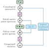 |
Fig. 1. Hierarchical representation of the Bayesian framework employed for diagnosing model misspecification and inferring the target parameters ω. The rounded green boxes denote probability distributions, whilst the purple squares represent deterministic functions. 𝒫(ω) is the prior on ω. 𝒯 is a deterministic function linking ω to θ. 𝒫(Φ|θ) denotes the probabilistic data model that maps the space of latent vectors θ to the survey space. The final layer, |

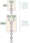 |
Fig. 2. Detailed representation of the BHM used in this study for the inference of cosmological parameters ω from galaxy surveys. The hidden-box model corresponds to the second dashed orange rectangle and defines the true (unknown) likelihood L(θ) when Φ = ΦO. The variables are ω (the target cosmological parameters), θ (the initial matter power spectrum), ψ (the nuisance parameters), o (the cosmological parameters, formally treated as nuisance parameters within the hidden-box), d (the full data vector containing the full galaxy count fields), Φ (the summary statistics), and |

Main variables, their generic role in the statistical framework, and their physical interpretation in this study.
In this work, the variables ω and θ are linked by a deterministic Boltzmann solver, the cosmic linear anisotropy solving system (CLASS, Blas et al. 2011), which associated with the deterministic function 𝒯 in the BHM. Alternative choices include the Code for Anisotropies in the Microwave Background (CAMB, Lewis & Challinor 2011), DIfferentiable Simulations for COsmology – Done with Jax (DISCO-DJ, Hahn et al. 2024), an emulator of cosmological power spectra (Spurio Mancini et al. 2022; Mootoovaloo et al. 2022) or a fitting function such as the Eisenstein-Hu fitting function (Eisenstein & Hu 1998; Campagne et al. 2023). In either case, 𝒯 is theoretically well-understood and numerically inexpensive compared to the potentially misspecified part of the BHM, which is the probabilistic simulator 𝒫(Φ|θ) linking the initial matter power spectrum θ to the simulated summary statistic Φ.
2.1.1. The top-level Bayesian problem
From a broad perspective, the cosmological inference problem considered here consists in updating prior knowledge 𝒫(ω) of the cosmological parameters ω through the Bayes rule
 (1)
(1)
based on observations ΦO from one or multiple cosmological probes, where the true, unknown likelihood with respect to the cosmological parameters is given by
 (2)
(2)
and the prior 𝒫(ω) stems from previous experiments and/or encodes physical constraints derived from theoretical considerations and heuristic rules. From this point onwards, to avoid assuming a parametric form for the likelihood Lω(ω), we employ ILI techniques based on a probabilistic forward model of the observable Φ. These techniques rely on comparing the simulated data, Φ, with the observations ΦO, which is difficult when the dimension P of the summarised data space is high. Consequently, the observed and simulated data must undergo an additional compression step, denoted by  in Figure 1.
2.1.2. The latent vector inference
To obtain a posterior for the initial matter power spectrum θ conditional on the observations ΦO, we consider the alternative inference problem defined by
 (3)
(3)
where
 (4)
(4)
is the true intermediate likelihood. We expect the inference of θ to be sensitive to most of the systematic effects of interest, as the initial matter power spectrum contains a wealth of information about the cosmological parameters ω (Peebles 1980). Harnessing our theoretical understanding of θ, we use the posterior 𝒫(θ|ΦO) as a diagnostic tool to examine how simulation- and observation-related systematic effects may affect the top-level Bayesian inference problem defined by Equation (2).
2.2. First step: Initial matter power spectrum inference
2.2.1. The power spectrum prior distribution
At wave number k, we define the latent vector as
 (5)
(5)
where P(k) is the initial matter power spectrum, and the normalisation function P0(k) is the Bardeen-Bond-Kaiser-Szalay (BBKS, Bardeen et al. 1986) power spectrum for some fiducial cosmological parameters ω0. The normalisation P0 plays no role in the statistical framework presented here and is introduced solely for numerical stability, as initial power spectra span several orders of magnitude across the range of scales considered.
We assume that, given a prior 𝒫(ω), a tight, physically-motivated prior on the initial matter power spectrum θ can be obtained by sampling from 𝒫(ω) and propagating the samples through the Boltzmann solver associated with the deterministic function 𝒯. That is,  , where
  is the Dirac measure centred on θ. Marginalising over ω yields:
 (6)
(6)
To obtain an explicit form for 𝒫(θ), we assume a Gaussian-distributed prior on the initial matter power spectrum, whose mean and covariance matrix can be estimated by drawing from Equation (6). We generate an ensemble of m simulated power spectra  , i ∈ ⟦1, m⟧, where ω(i) ∼ 𝒫(ω). The resulting prior reads
 (7)
(7)
where we introduced the notation ∥a∥B2 ≡ a⊺Ba, with
![Mathematical equation: $$ \begin{aligned} \boldsymbol{\hat{\theta }}_{\boldsymbol{\omega }} \equiv \mathrm{E}^m \left[ \boldsymbol{\theta }_{\boldsymbol{\omega }} \right] = \frac{1}{m}\sum _{i = 1}^{m} \boldsymbol{\theta }_{\boldsymbol{\omega }}^{(i)} \end{aligned} $$](/articles/aa/full_html/2025/07/aa53416-24/aa53416-24-eq18.gif) (8)
(8)
the mean of our prior, and where
![Mathematical equation: $$ \begin{aligned} \mathbf S&\equiv \frac{m}{m-1} \mathrm{E}^m \left[ (\boldsymbol{\theta }_{\boldsymbol{\omega }} - \boldsymbol{\hat{\theta }}_{\boldsymbol{\omega }})(\boldsymbol{\theta }_{\boldsymbol{\omega }} - \boldsymbol{\hat{\theta }}_{\boldsymbol{\omega }})^\intercal \right] \nonumber \\&= \frac{1}{m-1} \sum _{i = 1}^m (\boldsymbol{\theta }_{\boldsymbol{\omega }}^{(i)} - \boldsymbol{\hat{\theta }}_{\boldsymbol{\omega }}) (\boldsymbol{\theta }_{\boldsymbol{\omega }}^{(i)} - \boldsymbol{\hat{\theta }}_{\boldsymbol{\omega }})^\intercal \end{aligned} $$](/articles/aa/full_html/2025/07/aa53416-24/aa53416-24-eq19.gif) (9)
(9)
is the empirical prior covariance matrix. The symbol Em denotes the empirical mean computed from an ensemble of m samples.
Since evaluating the deterministic function 𝒯 is computationally inexpensive compared to the probabilistic simulator 𝒫(Φ|θ), m can be taken as large as necessary to ensure that the prior distribution 𝒫(θ) is well-sampled. In this work, we use m = 104.
2.2.2. The power spectrum posterior distribution
In the following, we adopt the approach introduced by Leclercq et al. (2019) to obtain a posterior on θ, with the key distinction that we formally treat the cosmological parameters o as additional nuisance parameters within the hidden-box model, over which we marginalise. In doing so, we rigorously account for the dependence of the mapping from initial matter power spectra to evolved dark matter density fields on the cosmological parameters.
Once realisations of θ, o, and ψ are specified, the output d ∈ ℝD of the simulation is a deterministic function 𝒮; that is, 𝒫(d|θ, o, ψ) = δdD(𝒮(θ, o, ψ)), where, again, δdD denotes the Dirac measure centred on d. Including the compression 𝒞 of the full data d to a summary statistic Φ, the hidden-box model can therefore be expressed as ℬ ≡ 𝒞° 𝒮, as illustrated in Figure 2. Marginalising over o and ψ, the exact likelihood given by Equation (4) reads
 (10)
(10)
which involves an intractable integral.
To overcome this difficulty, an inefficient yet insightful approach is to condition the probabilities on an ensemble of θ-dependent data realisations. For a given θ, consider an ensemble of K simulated summaries  with i ∈ ⟦1, K⟧, where K is arbitrary for now. Postulating an effective Gaussian likelihood yields
 ![Mathematical equation: $ \widetilde{L}^K(\boldsymbol{\theta}) = \exp\left[ \tilde{\ell}^K(\boldsymbol{\theta}) \right] $](/articles/aa/full_html/2025/07/aa53416-24/aa53416-24-eq22.gif) with the effective log-likelihood
with the effective log-likelihood  defined as
 (11)
(11)
where  is the empirical mean of the simulated summaries, defined by
![Mathematical equation: $$ \begin{aligned} \boldsymbol{\hat{\Phi }}_{\boldsymbol{\theta }} \equiv \mathrm{E}^K \left[ \boldsymbol{\Phi }_{\boldsymbol{\theta }} \right] = \frac{1}{K}\sum _{i = 1}^{K} \boldsymbol{\Phi }_{\boldsymbol{\theta }}^{(i)}, \end{aligned} $$](/articles/aa/full_html/2025/07/aa53416-24/aa53416-24-eq26.gif) (12)
(12)
and the estimators of the covariance matrix of  and its inverse are given by:
![Mathematical equation: $$ \begin{aligned} \frac{K-1}{K+1}\boldsymbol{\hat{\Sigma }}_{\boldsymbol{\theta }}^\prime&\equiv \mathrm{E}^K \left[ (\boldsymbol{\Phi }_{\boldsymbol{\theta }} - \boldsymbol{\hat{\Phi }}_{\boldsymbol{\theta }})(\boldsymbol{\Phi }_{\boldsymbol{\theta }} - \boldsymbol{\hat{\Phi }}_{\boldsymbol{\theta }})^\intercal \right] \nonumber \\&= \frac{1}{K} \sum _{i = 1}^K (\boldsymbol{\Phi }_{\boldsymbol{\theta }}^{(i)} - \boldsymbol{\hat{\Phi }}_{\boldsymbol{\theta }}) (\boldsymbol{\Phi }_{\boldsymbol{\theta }}^{(i)} - \boldsymbol{\hat{\Phi }}_{\boldsymbol{\theta }})^\intercal \,\mathrm{and} \nonumber \\ \frac{K+1}{K}\boldsymbol{\hat{\Sigma }}_{\boldsymbol{\theta }}^{\prime -1}&\equiv \alpha \,\boldsymbol{\hat{\Sigma }}_{\boldsymbol{\theta }}^{-1}, \end{aligned} $$](/articles/aa/full_html/2025/07/aa53416-24/aa53416-24-eq28.gif) (13)
(13)
respectively. The factor  arises from the assumption that
  follows an inverse-Wishart distribution (Hartlap et al. 2007); the
  factor originates from a derivation of
  based on a surrogate signal proposed in Leclercq et al. (2019), which motivates the Gaussian parametric form.
At this point, the numerical cost of computing  as given by Equation (11) is still prohibitively large when the full parameter space has to be explored: it requires K simulations per θ where an evaluation of the approximate likelihood is sought. The SELFI algorithm solves this issue by Taylor-expanding the full forward model at first order around an expansion point θ0, leveraging prior knowledge of the initial matter power spectrum so that the linearised model remains asymptotically exact around θ0. We define the expansion point as
 (14)
(14)
where ω0 is a vector of fiducial cosmological parameters.
The aforementioned approach translates into a linearisation of the mean data model around the initial matter power spectrum θ0. Namely, let o and ψ denote cosmological and nuisance parameters, δθ be a small vector in the parameter space; let X0 = (θ0, o, ψ), H = (δθ,0, 0), X = X0 + H. At first order in its first variable, ℬ(X) ≡ 𝒞° 𝒮(X) can be approximated by
 (15)
(15)
where ℬj(X) is the j-th component of ℬ(X) and ∂θ denotes the partial derivative with respect to the initial matter powerspectrum. Formally treating the cosmological parameters o intervening in the second layer of the BHM as a nuisance and marginalising over all nuisances yields
![Mathematical equation: $$ \begin{aligned} \mathbb{E} \left[ \boldsymbol{\Phi }_{\boldsymbol{\theta }} \right]&\equiv \int \mathcal{B} \left(\boldsymbol{\mathrm{X}}\right) \mathcal{P} (\mathbf o ) \mathcal{P} (\boldsymbol{\psi }) \, \mathrm{d}\mathbf o \,\mathrm{d}\boldsymbol{\psi } \nonumber \\&\simeq \int \left[\mathcal{B} \left(\boldsymbol{\mathrm{X}}_0\right) + \partial _\theta \mathcal{B} \left(\boldsymbol{\mathrm{X}}_0\right)\delta \boldsymbol{\theta }\right] \mathcal{P} (\mathbf o ) \mathcal{P} (\boldsymbol{\psi }) \, \mathrm{d}\mathbf o \,\mathrm{d}\boldsymbol{\psi } \nonumber \\&\simeq \mathbb{E} \left[ \mathcal{B} \left(\boldsymbol{\mathrm{X}}_0\right) \right] + \partial _\theta \mathbb{E} \left[ \mathcal{B} \left(\boldsymbol{\mathrm{X}}_0\right) \right] \cdot \delta \boldsymbol{\theta }, \end{aligned} $$](/articles/aa/full_html/2025/07/aa53416-24/aa53416-24-eq36.gif) (16)
(16)
under the assumption that the 𝔼 and ∂θ operators can be permuted in Equation (16), and where the expectation is taken with respect to the joint distribution of o and ψ. For any θ, the ensemble mean 𝔼[Φθ] can therefore be approximated by
 (17)
(17)
where δθ = θ − θ0, f0 ≡ EN0[Φθ0] is the empirical mean of the data model at the expansion point θ0 using N0 simulations for different phase and other nuisance realisations, and ∇θf0 is the empirical gradient of ℬ.
Further assuming the covariance matrix to be independent of θ close to the expansion point, that is  , and replacing the exact data model in Equation (11) with the linearised data model f, the SELFI effective likelihood is given by
 ![Mathematical equation: $ \widehat{L}^{N_0}(\boldsymbol{\theta}) = \exp\left[ \hat{\ell}^{N_0}_{\theta}(\boldsymbol{\theta}) \right] $](/articles/aa/full_html/2025/07/aa53416-24/aa53416-24-eq39.gif) with
with
 (18)
(18)
At the end of the day, SELFI approximates the average hidden-box model with its linearisation f around θ0 marginalised over the nuisance parameters. These assumptions, alongside the Gaussian effective likelihood assumption, solely impact the inference of the initial matter power spectrum θ, and do not affect the inference of the target cosmological parameters ω discussed later, except through data compression.
The SELFI likelihood defined by Equation (18) is fully characterised by f0, C0, and ∇θf0, which can all be evaluated through forward simulations. The numerical computation requires N0 simulations at the expansion point to evaluate f0 and C0. The gradient ∇θf0 can be evaluated using an analytical formula or auto-differentiation when available. In this work, we perform Nssimulations in each direction of the parameter space to empirically estimate ∇θf0 via first-order forward finite differences. The total number of simulations required is therefore Ntot = N0 + Ns × S simulations. N0 and Ns should be of the order of the dimensionality of the data space P, giving a total cost of 𝒪(≳P(S + 1)) model evaluations. If not chosen in advance, a precise value for N0 and Ns can be obtained by ensuring sufficient convergence of the covariance matrix and the gradients (see Appendix A) or by monitoring the convergence of the SELFI posterior.
To fully characterise the Bayesian problem, any prior 𝒫(θ) can be used, such as the prior naturally given by Equation (6). Any numerical technique such as MCMC can then be employed to explore the posterior using Equation (18), which does not require any additional evaluation of the hidden-box model. Remarkably, if the prior is Gaussian, then the SELFI effective posterior for the initial matter power spectrum is Gaussian and reads:
 (19)
(19)
with mean and covariance matrix given by
 (20)
(20)
![Mathematical equation: $$ \begin{aligned} \boldsymbol{\Gamma }&\equiv \left[ (\boldsymbol{\nabla }_{\theta } \mathbf f _0)^\intercal \, \mathbf C _0^{-1} \boldsymbol{\nabla }_{\theta } \mathbf f _0 + \mathbf S ^{-1} \right]^{-1}. \end{aligned} $$](/articles/aa/full_html/2025/07/aa53416-24/aa53416-24-eq43.gif) (21)
(21)
 is the difference between the prior mean and the expansion point. This result was derived by Leclercq et al. (2019) for the special case where the mean of the prior is equal to the expansion point; that is, Δ = 0. We provide the general derivation in Appendix B. To avoid inverting S in case it is ill-conditioned, one may equivalently opt for the alternative form:
![Mathematical equation: $$ \begin{aligned} \boldsymbol{\Gamma }\mathbf S ^{-1}\boldsymbol{\Delta }&= \left[ \mathbf S (\boldsymbol{\nabla }_{\theta } \mathbf f _0)^\intercal \, \mathbf C _0^{-1} \boldsymbol{\nabla }_{\theta } \mathbf f _0 + \mathbf I \right]^{-1}\boldsymbol{\Delta }, \end{aligned} $$](/articles/aa/full_html/2025/07/aa53416-24/aa53416-24-eq45.gif) (22)
(22)
![Mathematical equation: $$ \begin{aligned} \boldsymbol{\Gamma }&= \left[ \mathbf S (\boldsymbol{\nabla }_{\theta } \mathbf f _0)^\intercal \, \mathbf C _0^{-1} \boldsymbol{\nabla }_{\theta } \mathbf f _0 + \mathbf I \right]^{-1}\mathbf S . \end{aligned} $$](/articles/aa/full_html/2025/07/aa53416-24/aa53416-24-eq46.gif) (23)
(23)
2.2.3. Check for model misspecification
A sensitivity analysis of how systematic effects in the data model influence the posterior θ can be performed by recalculating the SELFI posterior mean γ using Equation (20) whilst varying the model of the systematic effect under investigation. This approach enables qualitative assessments of the impact of model misspecification on the posterior initial matter power spectrum, which can be interpreted in light of theoretical considerations. For a given posterior, as a simple quantitative check for model misspecification, we compute the Mahalanobis distance between the reconstruction γ and the prior distribution 𝒫(θ):
 (24)
(24)
We compare it to an ensemble of values of dM(θ, θ0|S) for simulations θ = 𝒯(ω), where ω is drawn from 𝒫(ω).
2.3. Second step: Implicit likelihood inference of the cosmological parameters
2.3.1. Score compression
The second step of the framework focuses on inferring the cosmological parameters ω based on the observations ΦO. As usual in ILI, the simulated and observed summaries must undergo an additional compression step to reduce their dimensionality. In essence, the compressed summaries  should closely approximate sufficient statistics of Φ, such that
  . Following the procedure described by Leclercq (2022), we assume, for compression only, that 𝒫(Φ|ω) is Gaussian-distributed:
 ![Mathematical equation: $ \mathcal{P}(\boldsymbol{\Phi}_{\mathrm{O}}|\boldsymbol{\omega}) \equiv \exp \left[ \hat{\ell}_\omega(\boldsymbol{\omega}) \right] $](/articles/aa/full_html/2025/07/aa53416-24/aa53416-24-eq50.gif) with
with  , where
![Mathematical equation: $$ \begin{aligned} -2 \hat{\ell }_\omega (\boldsymbol{\omega }) \equiv \log \left| 2\pi \mathbf C _0 \right| + \left||\boldsymbol{\Phi }_{\rm O} - \mathbf f \left[\mathcal{T} (\boldsymbol{\omega })\right]\right||^2_\mathbf{C _0^{-1}} \end{aligned} $$](/articles/aa/full_html/2025/07/aa53416-24/aa53416-24-eq52.gif) (25)
(25)
is the effective log-likelihood defined in the first part of the framework by Equation (18), which corresponds to the exact log-likelihood under the Gaussian assumption.
We consider the score function  , which is the gradient of the log-likelihood with respect to the parameters ω at a fiducial point in parameter space. This function is a sufficient statistic for the log-likelihood given by Equation (25) to linear order (Alsing & Wandelt 2018), making it a natural choice for data compression. Using ω0 as the fiducial point, a quasi maximum-likelihood estimator for the parameters is given by
  where the Fisher matrix
 ![Mathematical equation: $ \mathbf{F}_0=\mathbb{E}\left[\boldsymbol{\nabla} \hat{\ell}_\omega({\boldsymbol{\omega}_0}) \boldsymbol{\nabla}^\intercal \hat{\ell}_\omega({\boldsymbol{\omega}_0})\right] $](/articles/aa/full_html/2025/07/aa53416-24/aa53416-24-eq55.gif) represents the expected observed information, and the gradient of the log-likelihood is evaluated at ω0. Compression of ΦO to
represents the expected observed information, and the gradient of the log-likelihood is evaluated at ω0. Compression of ΦO to  yields N compressed statistics, which are optimal in the sense that they saturate the Fisher information content of the data at the expansion point under lenient assumptions provided by Alsing & Wandelt (2018).
Further assuming that the covariance C0 does not depend on the parameters (∇ωC0 = 0) around the expansion point, and using Equation (14), the compressor can be approximated by
![Mathematical equation: $$ \begin{aligned} \widetilde{\mathcal{C} }(\boldsymbol{\Phi }) \equiv \boldsymbol{\widetilde{\omega }} \equiv \boldsymbol{\omega }_0 + \mathbf F ^{-1}_0 \left[ (\boldsymbol{\nabla }_{\omega } \mathbf f _0)^\intercal \mathbf C _0^{-1} (\boldsymbol{\Phi } - \mathbf f _0) \right], \end{aligned} $$](/articles/aa/full_html/2025/07/aa53416-24/aa53416-24-eq57.gif) (26)
(26)
where the Fisher matrix is given by
![Mathematical equation: $$ \begin{aligned} \mathbf F _0 \equiv -\mathbb{E} \left[ \boldsymbol{\nabla }_{\omega } \boldsymbol{\nabla }_{\omega }\hat{\ell }_\omega ({\boldsymbol{\omega }_0}) \right] = (\boldsymbol{\nabla }_{\omega } \mathbf f _0)^\intercal \mathbf C _0^{-1} \boldsymbol{\nabla }_{\omega } \mathbf f _0, \end{aligned} $$](/articles/aa/full_html/2025/07/aa53416-24/aa53416-24-eq58.gif) (27)
(27)
with ∇ωf0 = ∇f0 ⋅ ∇ω𝒯(ω0) (Heavens et al. 2000; Alsing & Wandelt 2018). Alsing & Wandelt (2018) provide a more general data compression scheme which includes the case when the dependence of C0 on the parameter cannot be neglected.
At this point, C0 and ∇f0 have already been computed for the initial matter power spectrum inference with SELFI; and the gradient ∇ω𝒯(ω0) derived from the Boltzmann solver can easily be computed for instance by finite difference or using auto-differentiation (Hahn et al. 2024). We now have a BHM that maps the N target parameters, ω, to the same number N of compressed summaries,  , as summarised in Figure 1, which can be used to infer the target cosmological parameters using standard ILI techniques.
2.3.2. Implicit likelihood inference with a population Monte Carlo sampler
Every ILI method, such as ABC, requires a discrepancy measure to compare the compressed simulated summaries  with the observed summaries
  (Beaumont et al. 2002; Sunnåker et al. 2013). For this purpose, we re-used the Fisher matrix from Equation (27) to compute the Fisher-Rao distance between the compressed observed and simulated data, defined by:
 (28)
(28)
To infer the target parameters  given the observed summaries,
  , we relied on a simple yet theoretically well-motivated particle filter method, which is a variant introduced by Simola et al. (2021) of ABC-PMC. Unlike the basic ABC sampling strategy, known as implicit likelihood rejection sampling (Neumann 1951; Beaumont et al. 2002), and which does not take advantage of the information acquired during the sampling process, particle filters iteratively refine pools of candidates–referred to as particles, bringing them closer and closer to the true posterior distribution. Specifically, ABC-PMC methods gradually enhance the quality of the samples by updating the proposal distribution.
The ABC-PMC algorithm variant introduced by Simola et al. (2021) and employed here proceeds as follows. First, we set an initial acceptance threshold ϵ0, and generated an initial pool of J particles ![Mathematical equation: $ \Xi^{(0)} \equiv \left\{\boldsymbol{\omega}_i^{(0)}\right\}_{i\in [ [ 1,\,J ]] } $](/articles/aa/full_html/2025/07/aa53416-24/aa53416-24-eq65.gif) by drawing cosmological parameters from the proposal distribution π(0)(ω)≡𝒫(ω) until they satisfied
by drawing cosmological parameters from the proposal distribution π(0)(ω)≡𝒫(ω) until they satisfied  . This initial step is equivalent to an implicit likelihood rejection sampling stage with J accepted samples and a tolerance ϵ0.
To construct an intermediate proposal distribution π(1)(ω) and the corresponding approximate posterior, the method uses a Gaussian mixture distribution. We set initial weights wi(0) ≡ J−1. The initial multivariate Gaussian kernel functions are centred on ωi(0), with a common covariance matrix defined as twice the weighted sample covariance of the particles Ξ(0); that is,
 (29)
(29)
where  is the sample mean of the particles Ξ(0). The factor 2 arises from minimising the Kullback–Leibler divergence (Kullback & Leibler 1951) between the proposal and the target distribution (Beaumont et al. 2009). This leads to the updated proposal distribution
 (30)
(30)
where 𝒢(ω|μ,Σ) denotes the probability distribution function (PDF) of a Gaussian centred on μ with covariance matrix Σ, evaluated at ω.
In subsequent iterations t, the algorithm proceeds by drawing particles from the approximate posterior proposal distribution π(t)(ω) until they satisfy  for some ϵt < ϵt − 1. This results in the updated pool of particles
 ![Mathematical equation: $ \Xi^{(t)}=\left\{\boldsymbol{\omega}_i^{(t)}\right\}_{i\in [ [ 1,\,J ] ] } $](/articles/aa/full_html/2025/07/aa53416-24/aa53416-24-eq71.gif) , along with an updated proposal π(t + 1)(ω) given by the Gaussian mixture distribution
, along with an updated proposal π(t + 1)(ω) given by the Gaussian mixture distribution
 (31)
(31)
where the unnormalised importance weights are
 (32)
(32)
so that  . The covariance matrix Σ(t) is, again, defined as twice the weighted sample covariance of the particles Ξ(t). The resulting approximate posterior can thus be expressed as a kernel density estimator:
 (33)
(33)
where kh is the kernel (e.g. Rosenblatt 1956; Parzen 1962), and where we replaced the exponent (t) with ϵt to emphasise the dependence on the acceptance threshold. In this study, we used an isotropic Gaussian kernel with a smoothing parameter h. The particles were drawn from sequentially improving proposal distributions, with decreasing tolerances ϵ0 > ϵ1 > … > ϵT. The algorithm starts with an initial acceptance quantile q0, which is fixed by the initial tolerance ϵ0, and terminates when qT falls below a predetermined target quantile q. The target q sets the maximum allowable pointwise difference between posteriors at successive stages for the algorithm to be deemed converged. The rule for determining T and the choice of the decreasing sequence of tolerances are discussed in detail in Simola et al. (2021). The sequence is designed to ensure efficient sampling and to provide good exploration of the relevant regions of the parameter space. Starting from the initial acceptance quantile q0, subsequent tolerances were determined as follows:
![Mathematical equation: $$ \begin{aligned} \epsilon _t&= \displaystyle \min _{i \in [\![1, J ]\!]} \left\{ d_{\rm FR}\left(\widetilde{\mathcal{C} } \circ \mathcal{B} \left(\boldsymbol{\omega }_i^{(t-1)}\right), \widetilde{\boldsymbol{\omega }}_{\rm O}\right) \right\} , \end{aligned} $$](/articles/aa/full_html/2025/07/aa53416-24/aa53416-24-eq76.gif) (34)
(34)
 (35)
(35)
where  is a density ratio estimate of the posterior change between steps t − 1 and t. Notably, substantial differences between the approximate posteriors at stages t − 1 and t lead to a large shrinkage of the proposed tolerance ϵt + 1. The shrinkage in tolerance gradually decreases as the ABC posterior converges.
3. Data model of galaxy surveys
In the following, Model A refers to the correct, well-specified model used to generate the synthetic observations, whilst Model B refers to a misspecified model.
3.1. Initial power spectrum parametrisation
Throughout this work, we defined the initial density fluctuations and galaxy overdensity fields on a cubic equidistant grid with a comoving side length of 3.6 Gpc/h and 5123 voxels, spanning scales between ks, min = 1.75 × 10⁻³h/Mpc and ks, max = 7.74 × 10⁻¹ h/Mpc. We discretised the parameter space by evaluating the continuous normalised power spectra at S = 64 support wave numbers ks, yielding the vector θ defined by Equation (5). Between two consecutive support wave numbers, we interpolated power spectra P(k) using quintic splines. The first eight support wave numbers match the largest modes in the Fourier grid of our set-up. We manually distributed the remaining support wave numbers up to ks, max to ensure a small maximum relative error in the representation of initial matter power spectra across all wave numbers of the Fourier grid. We verified that, for all k below the grid’s Nyquist frequency, this set-up yielded a relative interpolation error below 0.14% for the fiducial power spectrum.
3.2. Gravitational evolution
The data model is a non-linear process meant to approximate the large variety of physical and observational phenomena at play in actual galaxy surveys. To generate dark matter overdensity fields for a given set of cosmological parameters, we essentially followed the procedure described by Leclercq et al. (2019). We assumed a flat ΛCDM cosmology (Blumenthal et al. 1984) and used the best fit of the Planck 2018 data, given in Table 2, as the fiducial cosmological parameters ω0.
Fiducial cosmological parameters ω0.
Given an initial matter power spectrum P(k), we generated a corresponding realisation of the initial matter density contrast field δi. For the gravitational evolution, we used theSIMBELMYNë cosmological solver (Leclercq et al. 2015). We populated the initial grid of 5123 voxels with 10243 dark matter particles arranged on a regular lattice. These particles were evolved via second order Lagrangian perturbation theory (2LPT) (Moutarde et al. 1991; Bouchet et al. 1995) up to redshift zLPT = 19, followed by N-body evolution with COLA (COmoving Lagrangian Acceleration, Tassev et al. 2013) from zLPT to z1 = 0.1500, both implemented within SIMBELMYNë. We performed the COLA evolution on a particle-mesh grid of 10243 voxels. We used 20 non-uniform time steps, which we distributed to ensure approximately linear scaling in the scale factor a while meeting the requirements imposed by our choice of mock galaxy populations. Specifically, the first 14 time steps were linearly spaced in a up to redshift z3 = 0.8182, followed by four time steps linearly spaced in a up to redshift z2 = 0.4925, and finally two additional time steps to reach z1 = 0.1500, corresponding to a scale factor of a = 0.8696.
The observer is positioned at one corner of the box, whereby they see one octant of the sky. Using the radial component vr of their final peculiar velocities with respect to the observer, the dark matter particles are placed in redshift space according to the non-linear mapping defined for each particle by
 (36)
(36)
where zcosmo is the true cosmological redshift, zpec is the redshift due to the peculiar velocity, zobs is the “observed” redshift of the particle and c is the speed of light. The particles are then assigned to a 5123-voxels grid using the cloud-in-cell scheme (Hockney & Eastwood 1988) to give the density contrast fields at redshift zi, denoted δzi, illustrated in the upper and middle rows of Figure 3.
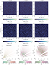 |
Fig. 3. Illustration of the galaxy survey data model used in this study. (Upper and middle rows) Slices through a realisation of the dark matter overdensity fields in real space (top) and redshift space (middle). The fields are evolved in time using N-body simulations, starting from a grid of Gaussian initial dark matter density fluctuations with power spectrum θgt, up to the redshift indicated above the corresponding panels. (Lower row) Observed galaxy number count fields for the three galaxy populations, each defined on a grid of 5123 cells. Light-cone effects are accounted for by using one effective redshift per galaxy population. Each slice passes through the observer located at the (0, 0, 0) corner of the box. |
3.3. Galaxy biasing
Galaxies are biased tracers of the underlying dark matter distribution (Kaiser 1984; Bardeen et al. 1986). The mapping from local dark matter overdensities to the galaxy density field is a crucial element in cosmological inferences, involving numerous physical processes. Multiple questions, such as halo formation and mergers, gas cooling, and stellar feedback (Desjacques et al. 2018), have to be addressed. Despite its inherent complexity, the highly non-linear process of galaxy formation can be accurately described by a small number of bias parameters on linear and quasi-linear scales, through a bias expansion in the matter density contrast and tidal fields. The parameters of this expansion often exhibit degeneracies with cosmological parameters, making the bias model critical in cosmological inferences, with the potential to either significantly enhance or severely bias the constraints on cosmological parameters (Barreira 2020; Barreira et al. 2020). Consequently, exploiting galaxy survey data beyond baryon acoustic oscillations (BAOs) requires careful modelling of galaxy biases (Barreira et al. 2021; Beyond-2pt Collaboration 2024), and there remains considerable scope for improving the bias models employed in cosmological analyses (Bartlett et al. 2024).
In this study, we focus on linear galaxy bias parameters, usually denoted b1 in the literature, and use our framework to assess the impact of these bias parameters on the SELFI posterior on the initial matter power spectrum. The same statistical framework can be applied to study the impact of higher-order local-in-matter density (LIMD) bias parameters or tidal biasparameters on the initial matter power spectrum reconstruction. We leave this exploration for future research. Hereafter, the first-order LIMD bias parameter for the i-th galaxy population gi is denoted bgi, to avoid confusion of bg2 and bg3 with higher order bias parameters.
We simulated three mock galaxy populations: one population of nearby bright galaxies and two populations of luminous red galaxies (LRGs). LRGs are slowly evolving galaxies that have been extensively studied; due to their high spatial densities and intrinsic brightness, they are among the most valuable tracers of the dark matter distribution (Eisenstein et al. 2001) in the Universe. Notably, subsamples of the 1.5 million spectra from the Baryon Oscillation Spectroscopic Survey (Eisenstein 2015) have been prominently used to study the large-scale structure of the Universe, proving able to measure the BAOs in their large-scale distribution (Eisenstein et al. 2005; Anderson et al. 2014). LRGs are notably the primary target of DESI within the redshift range 0.4 < z < 1.0 (Zhou et al. 2023).
We approximated light cone effects by using snapshots from the dark matter overdensity field at three distinct redshifts z1, z2, and z3, as input to the linear bias model to define the three populations of galaxies, where zi represents the effective redshift of the i-th galaxy population gi. According to the linear bias model, the normalised galaxy density ρgi for the galaxy population gi is therefore given in any cell x by:
 (37)
(37)
For simplicity, we used fixed values for the bgi parameters, given in Table 3. We emphasise that, given any prior distribution for these parameters, they could be treated as additional nuisances alongside ψ and marginalised over, without affecting the statistical framework presented in this article. To showcase the efficiency of our method for diagnosing systematic effects with high signal-to-noise ratio data, we made the simplifying assumption that  , effectively adopting a unit system where the mean number of galaxies per cell equals unity, which in turn affects the stochastic properties of the galaxy count fields, as detailed in Section 3.4. We further assumed that the contrast,
 (38)
(38)
Linear galaxy bias parameters used in this study.
could be observed directly, implying in particular that the mean number of galaxies per cell is perfectly known.
Values of the selection function parameters.
To simulate LRG populations, we based our approach on the measurements reported by Gil-Marıin et al. (2015), where the authors found b11.40(zeff)σ8(zeff) = 1.672 ± 0.060 and fσ8(zeff) = 0.597 for zeff = 0.57 (best fit of their full sample), yielding b11.40(zeff) = 2.80 ± 0.10. Motivated by the (b1, D) degeneracy between the linear galaxy bias and the growth factor at large scales, we assumed constant b1(z)D(z) within the relevant redshift range, yielding:
 (39)
(39)
For the two LRGs populations, g2 and g3, we applied Equation (39) to the mean redshift of each bin, used as the effective redshift to estimate an approximate ground truth linear bias (see Figure 4 and Table 3). For nearby galaxies, we used the measurements  and b1σ8(z1 = 0.15) = 1.20 ± 0.15 provided for a sample of high-bias galaxies at z < 0.2 by Howlett et al. (2015). Assuming
  (Bouchet et al. 1995), we obtained b1(z1 = 0.15)≃1.45. For Model A, we randomly selected the ground truth values in a ±0.02 interval around those given by the above equations. For Model B, the misspecified values were chosen manually. They are reported in Table 3.
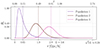 |
Fig. 4. Radial selection functions modelled as log-normal distributions in redshift (upper x axis) for the three mock galaxy populations. In the figure, the distributions are represented with respect to comoving distances (lower x axis) using the redshift-distance relation. The continuous lines represent the selection functions for the well-specified Model A, while the dotted lines represent the misspecified Model B, both defined by the values provided in Table 4. The small, percent-order difference between Models A and B renders the dotted curves nearly indistinguishable from the solid ones. The vertical dashed lines indicate the means of the log-normal distributions. |
3.4. Observational processes
The last step involves a virtual observation of the galaxy fields, accounting for observational effects expected in actual surveys. One such effect is dust extinction. Dust particles in the Milky Way and the intergalactic medium, presumably ejected by stars, absorb a significant portion of UV-to-near-infrared light, contaminating observations, causing reddening that must be corrected for (Galametz et al. 2017), and affecting the noise properties of the observed galaxies (Ho et al. 2015). The presence of gas and plasma in the intra- and extra-galactic medium introduces another known source of attenuation, as these media absorb, scatter, and re-emit a portion of incident radiation at longer wavelengths (Ménard et al. 2008; More et al. 2009).
These attenuation phenomena, along with contamination from bright stars, constitute complex and often correlated systematic effects (Boulanger et al. 1996) which can significantly impact nearly all cosmological measurements, from supernova distance estimates (Brout & Riess 2023) to photometric and spectroscopic galaxy surveys (Corasaniti 2006; Leistedt & Peiris 2014; Ho et al. 2015; Bovy et al. 2016). Consequently, considerable effort is devoted to accurately modelling and accounting for dust extinction in cosmological inference pipelines (e.g. Huterer et al. 2013; Jasche & Lavaux 2017; Karchev et al. 2024).
To obtain the simulated data from the galaxy contrast fields, we computed the three-dimensional survey response operators Wi. For each galaxy population gi, the corresponding operator is defined as the product of the radial selection function, Ri(r), and the angular survey mask and completeness function  for any line of sight
  ; that is,
 (40)
(40)
For the angular completeness  , we used a mask mimicking the wide sky coverage of stage-IV experiments, shown in Figure 5. We introduced additional linear extinction near the galactic plane up to 60° galactic latitude as a simple model of dust extinction. We also introduced 256 randomly positioned holes of angular diameter ∼0.1°, representing the masking of bright stars or other point sources contamination expected in galaxy surveys. Then, we projected the octant delineated by the light orchid triangle in Figure 5 onto the observed 5123 grid to define the survey mask. We modelled the radial selection functions as log-normal distributions in redshift, which approximately captures the expected behaviour over a range of redshifts (as in e.g. Gavazzi & Jaffe 1986). They are defined by
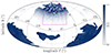 |
Fig. 5. Survey mask for the well-specified Model A. We added extinction linearly decreasing from 100% at the galactic plane to 0% at 60° galactic latitude (dash-dotted orchid line), along with 256 holes of approximately 0.1-degree radius (white crosses). The observed octant is delineated by the light orchid triangle. The colour scale represents the completeness function |

![Mathematical equation: $$ \begin{aligned} R_i(z)=\dfrac{c_i}{z\sigma _i\sqrt{2\,\pi }}\left[\exp \left({-\dfrac{(\ln {z}-\mu _i)^2}{2\,\sigma _i^2}}\right)\right], \end{aligned} $$](/articles/aa/full_html/2025/07/aa53416-24/aa53416-24-eq91.gif) (41)
(41)
where the constants σi and μi take different values for the three galaxy populations, and ci scales the amplitude of the signal. By analogy with the scaling of redshift uncertainties in typical photometric survey models (e.g. Laureijs et al. 2011), we defined the variance si of the log-normal selection functions in our data model as
 (42)
(42)
with an overall factor s = 0.1, where zi is the effective redshift of the i-th galaxy population. The Ri are defined in redshift using  and σi2 = ln(1+si2/zi2), and then mapped to distance space using tabulated values of the distance-redshift relation. The values of zi, si, and ci used for Models A and B are provided in Table 4; the corresponding profiles of the selection functions are illustrated in Figure 4.
We emulated the survey by generating galaxy excess number counts Nxgi for each cell x of the box across the three galaxy populations. To account for instrumental noise, the Nxgi were drawn from Gaussian distributions with means μxgi and standard deviations ςi, x,
 (43)
(43)
The mean μxgi ≡ Wi, xbgi δxzi characterises the expected number of galaxies based on Equation (38), where Wi, x is the value in the cell x of the three-dimensional response operator defined by Equation (40). The standard deviation is defined as  , where ς = 1 is the overall shot noise level. Setting
  in Equation (37) yields a mean galaxy number density of approximately 6 × 10⁻³ h3 Mpc−3 for the mock populations of LRGs, which is about an order of magnitude higher than the expected galaxy number density in actual surveys, for instance 5 × 10⁻⁴ h3 Mpc−3 in Berti et al. (2023). A slice through one realisation of the galaxy counts fields Ngi for each population gi is shown in Figure 3.
3.5. Summary statistics
The full data vectors d, consisting of the three 5123-dimensional galaxy count fields, are compressed into a summary statistic believed to contain relevant information about the cosmological parameters. In this study, we use the estimated power spectra of the observed and simulated fields, which is a standard choice in cosmological data analysis that has proven to be a powerful tool for constraining cosmological parameters (e.g. Tegmark et al. 2004; Ross et al. 2013). The transformation from the full data space to the space of observed summaries corresponds to the data compressor 𝒞 in the BHM of Figure 2.
For each galaxy population gi, following Leclercq et al. (2019), we define the binned data power spectrum as
![Mathematical equation: $$ \begin{aligned} P^{\mathrm{g}_i}(k_r) = \sum _{|\mathbf k | \in \left[k_r\pm \delta r\right]} \frac{\vert \widehat{N}_k^{\mathrm{g}_i}\vert ^2}{N_{k_r}-2}, \end{aligned} $$](/articles/aa/full_html/2025/07/aa53416-24/aa53416-24-eq97.gif) (44)
(44)
for kr − δr > 0, where  denotes the discrete Fourier transform of Ngi. Nkr represents the total number of Fourier modes within the wave number shell around kr. The −2 term arises from the assumption that the data power spectrum follows an inverse-Γ distribution with shape parameter Nkr/2 and scale parameter
  , corresponding to the Jeffreys prior for power spectra (Jasche et al. 2010). The summaries Φ are then defined as the concatenation of the three vectors Pgi, i = 1, 2, 3, corresponding to the three galaxy populations.
3.6. Synthetic observations
The ground truth cosmological parameters ωgt are drawn from the Planck 2018 prior (Planck Collaboration VI 2020). They are given up to the fourth decimal place in Table 5. We generate synthetic observations ΦO with the well-specified Model A, using
 (45)
(45)
Ground truth cosmological parameters.
as the input initial matter power spectrum, with ωgt given in Table 5, whilst fixing o = ωgt in the simulator. The synthetic observations are therefore obtained as
 (46)
(46)
4. Results
4.1. First step: Check for model misspecification
4.1.1. SELFI posteriors with the well- and misspecified models
We ran N0 = 500 and Ns × S = 640 simulations at and around the expansion point θ0 defined by Equation (14) and Table 2 to estimate f0 and ∇θf0, respectively. The simulated summaries used for estimating f0, along with their full covariance matrix, are displayed in Figure 6. Using these estimates, we computed the SELFI effective posterior 𝒫(θ|ΦO) based on Equations (20) and (21). From the simulated summaries and their covariance matrices alone, it is difficult to distinguish the well- and misspecified models, let alone identify the source of misspecification in Model B. More insight can be gained by examining the SELFI posteriors.
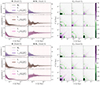 |
Fig. 6. Data intervening in the computation of the SELFI posterior. (Left panels) Observed and simulated summary statistics for Model A (well-specified; upper panel) and B (misspecified; lower panel). For each population, the simulated summaries are shown in grey and their means are represented as dotted coloured lines. The shaded areas correspond to ±2σ around their mean. The solid black line corresponds to the observations ΦO. The binning is indicated by the vertical dashed lines. Right panels: covariance matrices for Models A and B. For each (k, k′) entry, the colour scale represents the covariance between the k-th and k′-th modes. The diagonal blocs of the full covariance matrix correspond to the intra-population covariance; the extra-diagonal blocs correspond to the inter-populations covariances. |
The posterior initial matter power spectrum inferred with the well-specified Model A is represented in green in Figure 7. It is compatible with the truth across all scales, demonstrating the self-consistency of the SELFI assumptions. We further verify that this holds true for a wide range of observed data vectors derived from different sets of cosmological parameters, confirming the unbiasedness of the method (Appendix C.1). The posterior obtained with the misspecified Model B, in red in Figure 7, is implausible: it exhibits an excess of power of about ∼2σ with respect to the prior mean at the largest scales and a lack of power of similar amplitude at the smallest scales, where non-linear physics dominate.
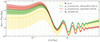 |
Fig. 7. Prior and SELFI posteriors for the initial matter power spectrum θ given the observations ΦO. The ground truth θgt is indicated by the dashed blue line. The prior and posterior means, θ0, γA and γB, are represented respectively by the yellow, green and red lines, along with their 2σ credible regions (shaded yellow, green, and red areas). The vertical dashed lines indicate the support wave numbers for the initial matter power spectrum representation. The posterior obtained with the well-specified Model A is unbiased over all scales, whilst the posterior obtained with the misspecified Model B exhibits an excess and a lack of power at the largest and smallest scales, respectively. |
As a quantitative check, Figure 8 depicts the Mahalanobis distances between 𝒫(θ) and the reconstructed mean power spectra γ for each model, computed using Equation (24), in comparison to those between 𝒫(θ) and 5000 random samples θn = 𝒯(ωn). Each ωn is drawn from the prior 𝒫(ω) on the cosmological parameters. The Mahalanobis distances aremultivariate analogues of the standard scores, accounting for correlations between the components, and measure the deviation of the reconstructions from the prior distribution. Large deviations suggest significant disagreement, prompting further investigation. We found that the distance for Model A, dM(γA, θ0|S) = 1.816, is much smaller than the distance for Model B, dM(γB, θ0|S) = 2.827. A larger distance does not necessarily imply a worse model, but hints at the presence of systematic effects. For comparison, the mean Mahalanobis distance from 𝒫(θ) to the 5000 θn samples is ⟨dM(θn,θ0|S)⟩n = 2.431. The disagreement between dM(γB, θ0|S) and the value typically observed from random samples, ⟨dM(θn,θ0|S)⟩n, highlights how percent-order variations in the modelling assumptions strongly influence the reconstruction of the initial matter power spectrum θ, pulling it away from the prior. This motivates a careful investigation of systematic effects, which we undertake in the following sections.
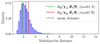 |
Fig. 8. Histogram of the Mahalanobis distances dM(θn, θ0|S) between the prior and 5000 power spectra θn ≡ 𝒯(ωn) sampled from Equation (6). The mean value is indicated by the vertical solid black line. The green and red lines indicate the distances from γA and γB to the prior, respectively. |
Additionally, since the prior given by Equation (9) embeds substantial information about the functional shape of the initial matter power spectrum, one might question how the SELFI algorithm performs with a less informative prior. Leclercq et al. (2019) demonstrated that a wiggle-less prior centred on θ0 ≡ 1ℝS enables precise recovery of initial features such as the BAOs up to mildly non-linear scales. Given the enhanced complexity of the data model employed here–incorporating extinction, point-source contamination, and radial selection effects, whilst using a lower mass-resolution–we successfully verified that the BAOs are still retrievable in this set-up using a prior agnostic to the BAOs, as is shown in Appendix C.2.
4.1.2. Impact of galaxy biases on the initial power spectrum reconstruction
Due to the non-linearity of the data model, the impact of the bias model on the posterior is in general out of reach of theoretical considerations. Linear galaxy biases, however, are expected to have a mostly scale-independent effect on the SELFI reconstruction γ of the initial matter power spectrum, as demonstrated in Appendix D based on qualitative considerations. This effect is observed on Figure 9a, which illustrates the impact of the linear galaxy bias parameters on the SELFI posterior distribution for the initial matter power spectrum. We considered a constant relative error in the ±2% range for the linear galaxy bias parameters of the three populations, as indicated by the colour scale. All scales experience a similar shift in standard deviations, which is consistent with the analytical expectations.
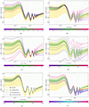 |
Fig. 9. Ensemble of SELFI posteriors for the initial matter power spectrum θ conditional on the observed data ΦO for different observational models, used to diagnose systematic effects. All the posteriors are derived from a single, common set of N-body simulations. They make it possible to disentangle individual systematic contributions by comparing their differential impact across the range of wave numbers spanned by the power spectra. The colour scales indicate the relative error associated with the systematic effects considered in each sub-figure. The solid yellow line denotes the prior mean θ0 and the ground truth θgt is indicated by the dashed blue line. The vertical dashed lines indicate the support wave numbers for the initial matter power spectrum representation. The 2σ credible regions for the prior and the posterior with the well-specified Model A correspond to the shaded yellow and green areas, respectively. The posterior means γ are represented by the coloured continuous lines for varying degrees of misspecification. For clarity, their corresponding credible regions have been omitted. (a) Impact of misspecified linear galaxy biases. (b) Impact of misspecified linear extinction. (c) Impact of misspecified redshifts. (d) Impact of misspecified selection function variances. (e) Impact of misspecified number of holes. (f) Impact of misspecified selection function variances (varying) under misspecified linear extinction (fixed). |
This demonstrates the ability of our framework to accurately diagnose the impact of systematic effects using the reconstructed initial matter power spectrum. We retrieve that the effect of misspecified linear galaxy bias parameters closely resembles a simple rescaling of the initial matter power spectrum by a constant factor, highlighting the well-known degeneracy between the linear galaxy bias parameters and the value of σ8 (Beutler et al. 2012; Arnalte-Mur et al. 2016; Desjacques et al. 2018; Repp & Szapudi 2020).
4.1.3. Impact of linear extinction, selection functions, punctual contaminations, and inaccurate redshifts
Even when the internal mechanisms of the forward model are known and well understood, assessing how a particular systematic effect influences the reconstruction solely through analytical considerations is often impractical. If an analytical expression can be derived, it may not be accurate due to correlations with other systematic effects, and its validity is likely to depend on the specificities of the hidden-box forward model. In such cases, we show that our framework makes it possible to conduct a thorough numerical investigation by reconstructing γ with Equation (20), whilst varying the values of the parameters involved in the model of the systematic effect. As a demonstration, we examine the impact of misspecified extinction near the galactic plane, misspecified selection functions, inaccurate redshifts, and punctual contaminations. All these numerical investigations rely on the same, common set of N-body simulations previously computed to obtain the posterior with Model A and already used to evaluate the effect of linear galaxy bias parameters in Section 4.1.2.
Figure 9b illustrates the effect of over- or underestimating the amount of extinction near the galactic plane. The colour scale represents the relative mean visibility between the misspecified and well-specified models, averaged over the three-dimensional survey window function. The extinction reduces the amplitude of small scales correlations; thus, overestimating extinction in the misspecified mask leads to a power deficit at small scales in the simulated summaries, shifting the reconstructed spectrum upwards. Conversely, underestimating extinction shifts the reconstructed spectrum downwards at small scales. At larger scales, excessive extinction in the misspecified mask introduces spurious fluctuations which are not retrieved in the observations, adding power to the largest k-modes and pushing the reconstruction downwards. As is shown in Figure 9b, the transition between these two regimes occurs at a constant scale, regardless of the degree of error in the extinction. This characteristic scale provides a means to distinguish the effects of extinction from other sources of systematic errors.
We emulated a systematic effect analogous to inaccurate redshifts due to line interlopers (e.g. Pullen et al. 2016; Addison et al. 2019; Massara et al. 2021) by increasing (or decreasing) the observed density of the central spectroscopic galaxy bin whilst correspondingly decreasing (or increasing) the densities of the two other populations, ensuring that the total density remained unchanged. An example of the resulting misspecified radial selection functions is shown in Figure 10. The resulting reconstructions, displayed in Figure 9c, demonstrate that even small, percent-level variations significantly affect the posterior on the initial matter power spectrum.
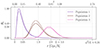 |
Fig. 10. Profiles of the well- and misspecified selection functions Ri for the three mock galaxy populations. The continuous lines represent the selection functions used in Model A. The dashed lines are derived by underestimating n1, 2(z) by 10% whilst maintaining ntot(z) constant. |
Figure 9d shows the impact of another source of systematic error associated with selection functions, specifically the impact of misspecified variances in the radial log-normal distributions. The result is comparable to that of misspecified galaxy bias parameters, though it is slightly more pronounced at smaller scales.
In complex data models displaying multiple putative sources of systematic effects alongside potentially many corresponding model parameters, it is crucial to know which effects are most likely to have a significant impact on the initial matter power spectrum, and should be prioritised for further investigation. Notably, some systematic effects may have a negligible impact on the initial matter power spectrum. Figure 9e illustrates the effect of misspecifying the number of holes in the survey mask in our set-up, using 0, 256, or all 512 holes defined at the beginning of the study, which represent the masking of bright stars or other point sources of contamination expected in cosmological surveys. The reconstruction appears largely unaffected by the number of holes, as their small angular size causes them to be overwhelmed by small-scale noise.
4.1.4. Joint impact of multiple systematic effects
Naturally, one is not restricted to studying individual systematic effects in isolation, and the SELFI posterior can be employed to explore how jointly misspecified observational effects influence the reconstructed initial matter power spectrum. This approach would be particularly beneficial for designing the data model of a real survey, enabling the assessment of the joint impact of different systematic effects on the cosmological inference whilst accounting for potential correlations between them. For example, Figure 9f shows the combined impact on the initial matter power spectrum of misspecified variances in the log-normal selection functions alongside incorrectly specified linearextinction.
Conversely, if a comprehensive study of multiple individual systematic effects has already been conducted, one can use it to disentangle their contributions when faced with a surprising posterior that warrants further investigation. For instance, if we obtain one of the reconstructions shown in Figure 9f, assuming unknown additive contributions of the five effects described in Section 4.1.3, we can easily disentangle individual contributions as follows. Shifting the reconstruction until it aligns with one of the characteristic scales associated with misspecified extinction or redshifts, we deduce that the systematic error most consistent with the observed reconstruction is a −10% error in the extinction, along with the corresponding error in the variance of the selection functions. As the model complexity increases, greater caution is required when interpreting the results, since multiple systematic effects can have degenerate impacts on the reconstructed power spectra. This underscores the importance of thoroughly investigating the influence of each individual systematic effect beforehand.
If known and unknown systematic effects are entangled, it remains possible to first identify the former using the characterisation presented in Figure 9. Running the framework while accounting for all known sources of systematic effects ensures that only unknown systematic effects and/or new physics remain to be characterised in the inferred initial matter power spectrum. Consequently, our framework has significant potential for detecting previously unknown systematic effects. This approach is conceptually distinct from that introduced by Porqueres et al. (2019), who identify and marginalise over unknown systematic effects within explicit likelihood inference.
4.1.5. Impact of the gravity solver
The gravity solver is a critical component of the data model. There is some flexibility in selecting the total number of time steps nsteps, dark matter particles Np, and the resolution of the particle-mesh grid used to compute the gravitational forces. Often, a trade-off must be made between the numerical cost of the resolution and the precision required by the observations and scientific objectives. The standard approach is to specify a target precision for the first or second-order statistics of the final dark matter overdensity fields and adjust the gravity solver parameters accordingly, based on convergence tests or comparisons with higher resolution simulations.
Unlike the systematic effects discussed in Sections 4.1.2, 4.1.3, and 4.1.4, obtaining multiple posteriors on the initial matter power spectrum for various configurations of the gravity solver implemented in the forward model requires re-running N-body simulations. However, the numerical cost of obtaining a single SELFI posterior for the initial matter power spectrum–𝒪(103) N-body simulations in this study–remains orders of magnitude lower than for the cosmological parameters–𝒪(105) N-body simulations in this study. Consequently, our framework presents further value for investigating the error caused by misspecified gravity models on the posterior initial matter power spectrum. Similarly, our framework could be employed to diagnose the effect of baryons in the hidden-box model based on the inferred initial matter power spectrum, provided one is willing to incur the numerical cost of incorporating baryonic physics into the simulator.
We refer to the error on the reconstructed initial matter power spectrum as the inverse error, as opposed to the direct error on the measured galaxy power spectra. We show that measuring this inverse error is particularly relevant for large-scale galaxy surveys: it highlights the sensitivity of the inference to the gravity solver parameters, which is not apparent from the direct error on the galaxy count fields.
Figures 11a and b illustrate the effect of using 10 instead of 20 time steps for the gravitational evolution with COLA. Whilst the direct error in the measured galaxy power spectra compared to Model A remains below 1% across all scales, the inverse error in the SELFI posterior exceeds 2% for k ≤ 4 ⋅ 10−3. This discrepancy arises due to the non-linearity of the inversion: small differences in the predicted galaxy power spectra between Models A and B can propagate into substantial biases in the posteriors after solving the inverse problem. As is shown in Figure 11b, the posterior rejects the ground truth by more than 2σ across most scales. The SELFI posterior is therefore highly sensitive to the time-stepping in the gravity solver. To achieve, for example, a 1% precision on the posterior, it is necessary to ensure an even higher precision in the galaxy count powerspectra.
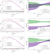 |
Fig. 11. Impact of the gravity solver parameters on the SELFI posterior. Panels (a, c, e) display the summary statistics Φ for the three galaxy count fields, comparing the well-specified Model A (dashed lines) with the misspecified model (solid lines). The lower parts of these panels show the relative error between the two models, with shaded regions corresponding to a 1% error margin. Panels (b, d, f) show the corresponding SELFI posteriors for the initial matter power spectrum θ, with the well-specified and misspecified models represented by green and indigo lines, respectively. (a) Example of summary statistics for a single realisation with nsteps = 10 (solid lines) as opposed to nsteps = 20 time steps for Model A (dashed lines) in the gravitational evolution with COLA. Although the direct error remains well below 1% across all scales, the inverse error on the SELFI posterior (b) reaches 2% at the largest scales, corresponding to a deviation greater than 1σ from the well-specified Model A. (c) Summary statistics using only the final snapshot at redshift z1 = 0.15 for the three mock galaxy populations, thereby neglecting light cone effects (solid lines). The forward error reaches 74% at the largest scales for the most distant galaxy population, and the corresponding SELFI posterior (d) significantly rejects the ground truth across all scales. (e) Summary statistics using a pure 2LPT gravity model instead of N-body simulations to define the galaxy populations (solid lines). The forward error reaches ∼7% at the smallest scale, and the ground truth is significantly rejected by the SELFI posterior (f), which deviates by more than 2σ compared to Model A at the largest scales. |
Similarly, Figures 11c and 11d highlight the importance of accounting for light cone effects in the forward model: the SELFI posterior consistently rejects the ground truth when all three galaxy populations are defined from the snapshot at redshift z1 = 0.15, compared to using z1, z2, and z3 in Model A. Since the cosmological structure is less evolved at higher redshifts, this results in overestimating the measured power spectrum amplitude for the two most distant galaxy populations, which pushes the SELFI posterior downwards at all scales. We note that this effect is highly degenerate with that of misspecified galaxy biases. Both risk biasing the value of σ8 inferred from the data if not properly accounted for.
Strikingly, Figure 11e and 11f show that using 2LPT instead of COLA in the forward model significantly biases the posterior on the initial matter power spectrum. This arises because the range of scales considered in this study extends well beyond klin ≃ 0.15 h/Mpc, commonly considered as the smallest scale of the linear regime (e.g. Colless et al. 2001), up to kmax ≃ 0.4 h/Mpc. Within the SELFI framework, all scales are coupled by the non-linearity. Over-prediction of small-scale power by 2LPT (due to the mass resolution) results in under-prediction of large scale power to fit the data. Furthermore, since the number of small-scale modes vastly exceeds that of large-scale modes, the posterior computation sacrifices large scale accuracy to fit small scales. The forward error on the galaxy count power spectra reaches ∼7% at the smallest scales, and the SELFI posterior rejects the ground truth by almost 2σ across most scales. This underscores the necessity of employing fully non-linear gravity solvers to accurately extract small-scale information from large-scale galaxy surveys.
4.2. Second step: Cosmological parameters
After checking for model misspecification, the second step of the framework consists of inferring the target cosmological parameters, ω, given the compressed summaries  . For score compression, we re-used the estimates f0 and ∇θf0 computed in the first step, and estimate the gradient ∇𝒯 of CLASS at the fiducial cosmological parameters
  using fifth order finite differences. To perform the inference, we use the ELFIpackage (Lintusaari et al. 2018), which implements the variant of ABC-PMC proposed by Simola et al. (2021) and discussed in Section 2.3.2.
To reduce computational costs, in this study, we inferred only Ωm, Ωb, nS, and σ8 whilst fixing h to the ground truth given in Table 5. This choice was further motivated by the fact that our data model carries no additional information beyond the prior concerning the value of h. For practical purposes, we used nine distinct ABC-PMC populations of 64 particles each, aggregating the J = 576 final samples and corresponding weights to obtain a posterior distribution of (Ωm, Ωb, σ8, nS). Figure 12 shows the posteriors obtained using a kernel density estimate with the J weighted accepted samples. The shaded yellow area corresponds to 2σ credible contours on the prior. The posterior with the well-specified Model A is shown in green; it is unbiased for all cosmological parameters.
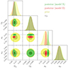 |
Fig. 12. Prior 𝒫(ω) (yellow) and posterior |


Replacing the accurate data Model A with the misspecified Model B for ABC-PMC yields the posterior in red. This substitution results in over-concentrating the posterior distributions of σ8, Ωm, and nS, and introduces a bias exceeding 2σ in the (σ8, Ωm) plane. The bias in the marginal posterior of σ8 is to be expected in light of the well-known degeneracy between σ8 and galaxy bias parameters (Beutler et al. 2012; Arnalte-Mur et al. 2016; Desjacques et al. 2018; Repp & Szapudi 2020).
5. Discussion and conclusion
We have presented a method for thoroughly assessing individual or combined systematic effects in galaxy surveys using the initial matter power spectrum. We provide a practical guide for evaluating the impact of various systematic effects, demonstrated using a spectroscopic galaxy survey model through a quantitative assessment of the effect of misspecified linear galaxy biases, extinction near the galactic plane, selection functions, punctual contaminations, inaccurate redshifts, and imprecise gravity solver.
The method introduced in this study offers a Bayesian framework for addressing model misspecification in field-based implicit-likelihood cosmological inference. Notably, we have shown that even small, percent-level errors can significantly skew cosmological inferences derived from galaxy clustering probes. This was illustrated by a bias exceeding 2σ in the (σ8, Ωm) plane (Figure 12), which we were able to detect and correct (Figures 7 and 9) prior to inferring the cosmological parameters. Correct identification of systematic effects is crucial for accurately measuring primordial features of the Universe, such as non-Gaussianities–a major scientific goal of next-generation galaxy surveys (Andrews et al. 2023). Our method could serve as a critical tool for field-based ILI of these primordial features.
Our approach primarily centres on systematic effects that influence the initial matter power spectrum reconstruction. While we have assumed that the inferred spectrum serves as a reliable proxy for cosmological parameters, there may be systematic effects that do not affect the initial matter power spectrum yet still introduce biases in cosmological inferences. Such effects fall outside the current scope of this framework. In this paper, we assumed fixed deterministic linear galaxy bias parameters, but scale-dependent or non-linear biasmodels could be incorporated within the same framework. Addressing model misspecification for more sophisticated bias models would be particularly relevant for the inference of primordial non-Gaussianities. If a prior distribution of the bias values is available, they can be treated as additional nuisance parameters alongside ψ and marginalised over without altering the statistical framework presented here. Alternatively, they could be treated as additional input parameters alongside θ and inferred jointly with the initial matter power spectrum. These avenues remain for future investigation.
Potential extensions of the method include incorporating higher-order summary statistics from the full galaxy count fields into the inference (Gil-Marıin et al. 2015; Philcox & Ivanov 2022), which provide valuable information, for instance for constraining dark energy (Fazolo et al. 2022). Other options include using wavelet scattering transform coefficients (Régaldo-Saint Blancard et al. 2024), and additional cosmological probes such as peculiar velocity tracers (Prideaux-Ghee et al. 2023). The compression step could be improved by using information-maximising neural networks (Charnock et al. 2018; Makinen et al. 2024; Lanzieri et al. 2024), which complement physically motivated summary statistics. These beyond 2-pt approaches are particularly relevant for extracting the maximum amount of information from upcoming galaxy surveys and could reveal additional sources of systematic effects which should be accounted for in cosmological inferences based on these summaries (Beyond-2pt Collaboration 2024).
In conclusion, we have proposed a method to address the issue of model misspecification in implicit likelihood, field-based cosmological inferences. It enables a comprehensive investigation of both simulation- and observation-related systematic effects in galaxy surveys, leveraging both theoretical insights and prior knowledge of the initial matter power spectrum. We demonstrated the effectiveness of this method by quantifying the impact of various systematic effects on the inferred initial matter power spectrum. Furthermore, we emphasised the importance of using an accurate model for gravitational evolution within the hidden-box model: our results indicate that pure 2LPT is insufficient for the range of scales considered in this study, which is k ∈ [1.75×10⁻³, 4.47×10⁻¹] h/Mpc. Our framework can be used with any hidden-box model of galaxy surveys developed for cosmological inference pipelines, making it a versatile tool for addressing model misspecification in cosmological data analysis. It has the potential to significantly enhance the robustness of cosmological inferences from upcoming galaxy surveys such as DESI, Euclid, and LSST, for which the complexity of data models and the number of systematic effects will be substantial.
Data availability
This study relies on the pySELFI implementation of the SELFI (Leclercq et al. 2019) algorithm, which is publicly available at pyselfi.florent-leclercq.eu.. The gravitational evolution is performed using a modified version of the publicly available SIMBELMYNë cosmological solver (https://bitbucket.org/florent-leclercq/simbelmyne, Leclercq et al. 2015). The code and data underlying this paper, including the hidden-box model of galaxy surveys described in the article and routines to perform the inference using our framework in a cluster environment, are publicly available at github.com/hoellin/selfisys_public.
If the likelihood of the model has an explicit form, explicit likelihood techniques may also be used for the second step.
Acknowledgments
We thank Chloé Barjou-Delayre, Guilhem Lavaux, Gary Mamon, Nhat-Minh Nguyen and Fabian Schmidt for useful discussions and feedback to enhance this manuscript. The work has made use of the Infinity Cluster hosted by the Institut d’Astrophysique de Paris. We appreciate the efforts of Stéphane Rouberol for running the cluster smoothly. FL and TH acknowledge financial support from the Agence Nationale de la Recherche (ANR) through the grant INFOCW, under reference ANR-23-CE46-0006-01. FL and TH acknowledge financial support from the Simons Collaboration on “Learning the Universe”. This work was done within the Aquila Consortium (https://www.aquila-consortium.org/).
References
- Addison, G. E., Bennett, C. L., Jeong, D., Komatsu, E., & Weiland, J. L. 2019, ApJ, 879, 15 [NASA ADS] [CrossRef] [Google Scholar]
- Albrecht, A., Bernstein, G., Cahn, R., et al. 2006, ArXiv e-prints [arXiv:astro-ph/0609591] [Google Scholar]
- Alsing, J., & Wandelt, B. 2018, MNRAS, 476, L60 [NASA ADS] [CrossRef] [Google Scholar]
- Alsing, J., Heavens, A., Jaffe, A. H., et al. 2016, MNRAS, 455, 4452 [Google Scholar]
- Alsing, J., Wandelt, B., & Feeney, S. 2018, MNRAS, 477, 2874 [NASA ADS] [CrossRef] [Google Scholar]
- Alsing, J., Charnock, T., Feeney, S., & Wandelt, B. 2019, MNRAS, 488, 4440 [Google Scholar]
- Anderson, L., Aubourg, É., Bailey, S., et al. 2014, MNRAS, 441, 24 [Google Scholar]
- Andrews, A., Jasche, J., Lavaux, G., & Schmidt, F. 2023, MNRAS, 520, 5746 [Google Scholar]
- Arnalte-Mur, P., Vielva, P., Martínez, V. J., et al. 2016, JCAP, 2016, 005 [Google Scholar]
- Ayçoberry, E., Ajani, V., Guinot, A., et al. 2023, A&A, 671, A17 [NASA ADS] [CrossRef] [EDP Sciences] [Google Scholar]
- Balkenhol, L., Dutcher, D., Spurio Mancini, A., et al. 2023, Phys. Rev. D, 108, 023510 [NASA ADS] [CrossRef] [Google Scholar]
- Bardeen, J. M., Bond, J. R., Kaiser, N., & Szalay, A. S. 1986, ApJ, 304, 15 [Google Scholar]
- Barreira, A. 2020, JCAP, 2020, 031 [CrossRef] [Google Scholar]
- Barreira, A., Cabass, G., Lozanov, K. D., & Schmidt, F. 2020, JCAP, 2020, 049 [Google Scholar]
- Barreira, A., Lazeyras, T., & Schmidt, F. 2021, JCAP, 2021, 029 [CrossRef] [Google Scholar]
- Bartlett, D. J., Ho, M., & Wandelt, B. D. 2024, ApJ, 977, L44 [Google Scholar]
- Beaumont, M. A., Zhang, W., & Balding, D. J. 2002, Genetics, 162, 2025 [Google Scholar]
- Beaumont, M. A., Cornuet, J.-M., Marin, J.-M., & Robert, C. P. 2009, Biometrika, 96, 983 [CrossRef] [Google Scholar]
- Berti, A. M., Dawson, K. S., & Dominguez, W. 2023, ApJ, 954, 131 [Google Scholar]
- Beutler, F., Blake, C., Colless, M., et al. 2012, MNRAS, 423, 3430 [NASA ADS] [CrossRef] [Google Scholar]
- Beyond-2pt Collaboration 2024, ArXiv e-prints [arXiv:2405.02252] [Google Scholar]
- Blas, D., Lesgourgues, J., & Tram, T. 2011, JCAP, 2011, 034 [Google Scholar]
- Blumenthal, G. R., Faber, S. M., Primack, J. R., & Rees, M. J. 1984, Nature, 311, 517 [Google Scholar]
- Bouchet, F. R., Colombi, S., Hivon, E., & Juszkiewicz, R. 1995, A&A, 296, 575 [NASA ADS] [Google Scholar]
- Boulanger, F., Abergel, A., Bernard, J. P., et al. 1996, A&A, 312, 256 [Google Scholar]
- Bovy, J., Rix, H.-W., Green, G. M., Schlafly, E. F., & Finkbeiner, D. P. 2016, ApJ, 818, 130 [Google Scholar]
- Brehmer, J., Louppe, G., Pavez, J., & Cranmer, K. 2018, ArXiv e-prints [arXiv:1805.12244] [Google Scholar]
- Brout, D., & Riess, A. 2023, ArXiv e-prints [arXiv:2311.08253] [Google Scholar]
- Campagne, J.-E., Lanusse, F., Zuntz, J., et al. 2023, Open J. Astrophys., 6, 15 [NASA ADS] [CrossRef] [Google Scholar]
- Carreres, B., Bautista, J. E., Feinstein, F., et al. 2023, A&A, 674, A197 [NASA ADS] [CrossRef] [EDP Sciences] [Google Scholar]
- Charnock, T., Lavaux, G., & Wandelt, B. D. 2018, Phys. Rev. D, 97, 083004 [NASA ADS] [CrossRef] [Google Scholar]
- Colless, M., Dalton, G., Maddox, S., et al. 2001, MNRAS, 328, 1039 [Google Scholar]
- Corasaniti, P. S. 2006, MNRAS, 372, 191 [Google Scholar]
- Cranmer, K., Brehmer, J., & Louppe, G. 2020, Proc. Natl. Acad. Sci., 117, 30055 [Google Scholar]
- Davis, T. M., Hui, L., Frieman, J. A., et al. 2011, ApJ, 741, 67 [NASA ADS] [CrossRef] [Google Scholar]
- DESI Collaboration 2016, ArXiv e-prints [arXiv:1611.00036] [Google Scholar]
- Desjacques, V., Jeong, D., & Schmidt, F. 2018, Phys. Rep., 733, 1 [Google Scholar]
- Ding, S., Lavaux, G., & Jasche, J. 2024, A&A, 690, A236 [NASA ADS] [CrossRef] [EDP Sciences] [Google Scholar]
- Doeser, L., Jamieson, D., Stopyra, S., et al. 2024, MNRAS, 535, 1258 [NASA ADS] [CrossRef] [Google Scholar]
- Duane, S., Kennedy, A. D., Pendleton, B. J., & Roweth, D. 1987, Phys. Lett. B, 195, 216 [CrossRef] [Google Scholar]
- Eisenstein, D. 2015, APS Meeting Abstracts, 2015, Z2.001 [Google Scholar]
- Eisenstein, D. J., & Hu, W. 1998, ApJ, 496, 605 [Google Scholar]
- Eisenstein, D. J., Annis, J., Gunn, J. E., et al. 2001, AJ, 122, 2267 [Google Scholar]
- Eisenstein, D. J., Zehavi, I., Hogg, D. W., et al. 2005, ApJ, 633, 560 [Google Scholar]
- Euclid Collaboration (Blanchard, A., et al.) 2020, A&A, 642, A191 [NASA ADS] [CrossRef] [EDP Sciences] [Google Scholar]
- Euclid Collaboration (Mellier, Y., et al.) 2025, A&A, 697, A1 [Google Scholar]
- Fazolo, R. E., Amendola, L., & Velten, H. 2022, Phys. Rev. D, 105, 103521P [Google Scholar]
- Frazier, D. T., Robert, C. P., & Rousseau, J. 2017, ArXiv e-prints [arXiv:1708.01974] [Google Scholar]
- Galametz, A., Saglia, R., Paltani, S., Apostolakos, N., & Dubath, P. 2017, A&A, 598, A20 [NASA ADS] [CrossRef] [EDP Sciences] [Google Scholar]
- Gavazzi, G., & Jaffe, W. 1986, ApJ, 310, 53 [Google Scholar]
- Gil-Marıin, H., Noreña, J., Verde, L., et al. 2015, MNRAS, 451, 539 [CrossRef] [Google Scholar]
- Glanville, A., Howlett, C., & Davis, T. M. 2021, MNRAS, 503, 3510 [NASA ADS] [CrossRef] [Google Scholar]
- Goldstein, S., Park, M., Raveri, M., Jain, B., & Samushia, L. 2023, Phys. Rev. D, 107, 063530 [Google Scholar]
- Hahn, O., List, F., & Porqueres, N. 2024, JCAP, 2024, 063 [Google Scholar]
- Hartlap, J., Simon, P., & Schneider, P. 2007, A&A, 464, 399 [NASA ADS] [CrossRef] [EDP Sciences] [Google Scholar]
- Heavens, A. F., Jimenez, R., & Lahav, O. 2000, MNRAS, 317, 965 [NASA ADS] [CrossRef] [Google Scholar]
- Ho, S., Agarwal, N., Myers, A. D., et al. 2015, JCAP, 2015, 040 [CrossRef] [Google Scholar]
- Ho, M., Bartlett, D. J., Chartier, N., et al. 2024, Open J. Astrophys., 7, 54 [NASA ADS] [CrossRef] [Google Scholar]
- Hockney, R. W., & Eastwood, J. W. 1988, Computer Simulation Using Particles (Taylor& Francis Group) [Google Scholar]
- Howlett, C., Ross, A. J., Samushia, L., Percival, W. J., & Manera, M. 2015, MNRAS, 449, 848 [NASA ADS] [CrossRef] [Google Scholar]
- Huterer, D., Cunha, C. E., & Fang, W. 2013, MNRAS, 432, 2945 [Google Scholar]
- Ishida, E. E., Vitenti, S. D., Penna-Lima, M., et al. 2015, Astron. Comput., 13, 1 [Google Scholar]
- Ivezić, Ž., Kahn, S. M., Tyson, J. A., et al. 2019, ApJ, 873, 111 [Google Scholar]
- Jasche, J., & Lavaux, G. 2017, A&A, 606, A37 [NASA ADS] [CrossRef] [EDP Sciences] [Google Scholar]
- Jasche, J., & Lavaux, G. 2019, A&A, 625, A64 [NASA ADS] [CrossRef] [EDP Sciences] [Google Scholar]
- Jasche, J., Kitaura, F. S., Wandelt, B. D., & Enßlin, T. A. 2010, MNRAS, 406, 60 [NASA ADS] [CrossRef] [Google Scholar]
- Jasche, J., & Wandelt, B. D. 2013, MNRAS, 432, 894 [Google Scholar]
- Kaiser, N. 1984, ApJ, 284, L9 [NASA ADS] [CrossRef] [Google Scholar]
- Karchev, K., Grayling, M., Boyd, B. M., et al. 2024, MNRAS, 530, 3881 [Google Scholar]
- Kim, A. G., Linder, E. V., Miquel, R., & Mostek, N. 2004, MNRAS, 347, 909 [Google Scholar]
- Kitching, T. D., Taylor, A. N., & Heavens, A. F. 2008, MNRAS, 389, 173 [NASA ADS] [CrossRef] [Google Scholar]
- Kitching, T. D., Verde, L., Heavens, A. F., & Jimenez, R. 2016, MNRAS, 459, 971 [Google Scholar]
- Kostić, A., Nguyen, N.-M., Schmidt, F., & Reinecke, M. 2023, JCAP, 2023, 063 [Google Scholar]
- Kullback, S., & Leibler, R. A. 1951, Ann. Math. Stat., 22, 79 [CrossRef] [Google Scholar]
- Laureijs, R., Amiaux, J., Arduini, S., et al. 2011, ArXiv e-prints [arXiv:1110.3193] [Google Scholar]
- Lanzieri, D., Zeghal, J., Makinen, T. L., et al. 2024, ArXiv e-prints [arXiv:2407.10877] [Google Scholar]
- Leclercq, F. 2018, Phys. Rev. D, 98, 063511 [NASA ADS] [CrossRef] [Google Scholar]
- Leclercq, F. 2022, Phys. Sci. Forum, 5, 4 [Google Scholar]
- Leclercq, F., Enzi, W., Jasche, J., & Heavens, A. 2019, MNRAS, 490, 4237 [NASA ADS] [CrossRef] [Google Scholar]
- Leclercq, F., Jasche, J., & Wandelt, B. 2015, JCAP, 2015, 015 [CrossRef] [Google Scholar]
- Leistedt, B., & Peiris, H. V. 2014, MNRAS, 444, 2 [Google Scholar]
- Lewis, A., & Challinor, A. 2011, Astrophysics Source Code Library [record ascl:1102.026] [Google Scholar]
- Lintusaari, J., Gutmann, M. U., Dutta, R., Kaski, S., & Corander, J. 2017, Syst. Biol., 66, e66 [Google Scholar]
- Lintusaari, J., Vuollekoski, H., Kangasrääsiö, A., et al. 2018, J. Mach. Learn. Res., 19, 1 [Google Scholar]
- Liu, D. C., & Nocedal, J. 1989, Math. Progr., 45, 503 [CrossRef] [Google Scholar]
- Loureiro, A., Whiteway, L., Sellentin, E., et al. 2023, Open J. Astrophys., 6, 6 [CrossRef] [Google Scholar]
- LSST Dark Energy Science Collaboration 2012, ArXiv e-prints [arXiv:1211.0310] [Google Scholar]
- Makinen, T. L., Charnock, T., Alsing, J., & Wandelt, B. D. 2021, JCAP, 2021, 049 [CrossRef] [Google Scholar]
- Makinen, T. L., Heavens, A., Porqueres, N., et al. 2024, ArXiv e-prints [arXiv:2407.18909] [Google Scholar]
- Massara, E., Ho, S., Hirata, C. M., et al. 2021, MNRAS, 508, 4193 [NASA ADS] [CrossRef] [Google Scholar]
- Meiksin, A., White, M., & Peacock, J. A. 1999, MNRAS, 304, 851 [NASA ADS] [CrossRef] [Google Scholar]
- Ménard, B., Nestor, D., Turnshek, D., et al. 2008, MNRAS, 385, 1053 [Google Scholar]
- Metropolis, N., Rosenbluth, A. W., Rosenbluth, M. N., Teller, A. H., & Teller, E. 1953, J. Chem. Phys., 21, 1087 [Google Scholar]
- Mishra-Sharma, S., Alonso, D., & Dunkley, J. 2018, Phys. Rev. D, 97, 123544 [Google Scholar]
- Modi, C., Lanusse, F., & Seljak, U. 2021, Astron. Comput., 37, 100505 [NASA ADS] [CrossRef] [Google Scholar]
- Mootoovaloo, A., Jaffe, A. H., Heavens, A. F., & Leclercq, F. 2022, Astron. Comput., 38, 100508 [NASA ADS] [CrossRef] [Google Scholar]
- More, S., Bovy, J., & Hogg, D. W. 2009, ApJ, 696, 1727 [Google Scholar]
- Moutarde, F., Alimi, J. M., Bouchet, F. R., Pellat, R., & Ramani, A. 1991, ApJ, 382, 377 [Google Scholar]
- Neumann, V. 1951, Notes by GE Forsythe, 36 [Google Scholar]
- Nguyen, N.-M., Schmidt, F., Lavaux, G., & Jasche, J. 2021, JCAP, 2021, 058 [Google Scholar]
- Nguyen, N.-M., Schmidt, F., Tucci, B., Reinecke, M., & Kostić, A. 2024, Phys. Rev. Lett., 133, 221006 [CrossRef] [Google Scholar]
- Parzen, E. 1962, Ann. Math. Stat., 33, 1065 [Google Scholar]
- Peebles, P. J. E. 1980, The Large-scale Structure of the Universe (Princeton: Princeton University Press) [Google Scholar]
- Philcox, O. H. E., & Ivanov, M. M. 2022, Phys. Rev. D, 105, 043517 [CrossRef] [Google Scholar]
- Planck Collaboration VI. 2020, A&A, 641, A6 [NASA ADS] [CrossRef] [EDP Sciences] [Google Scholar]
- Porqueres, N., Kodi Ramanah, D., Jasche, J., & Lavaux, G. 2019, A&A, 624, A115 [NASA ADS] [CrossRef] [EDP Sciences] [Google Scholar]
- Porqueres, N., Heavens, A., Mortlock, D., & Lavaux, G. 2022, MNRAS, 509, 3194 [Google Scholar]
- Prideaux-Ghee, J., Leclercq, F., Lavaux, G., Heavens, A., & Jasche, J. 2023, MNRAS, 518, 4191 [Google Scholar]
- Pullen, A. R., Hirata, C. M., Doré, O., & Raccanelli, A. 2016, PASJ, 68, 12 [NASA ADS] [CrossRef] [Google Scholar]
- Ramanah, D. K., Lavaux, G., Jasche, J., & Wandelt, B. D. 2019, A&A, 621, A69 [NASA ADS] [CrossRef] [EDP Sciences] [Google Scholar]
- Régaldo-Saint Blancard, B., Hahn, C., Ho, S., et al. 2024, Phys. Rev. D, 109, 083535 [CrossRef] [Google Scholar]
- Repp, A., & Szapudi, I. 2020, MNRAS, 498, L125 [NASA ADS] [CrossRef] [Google Scholar]
- Rosenblatt, M. 1956, Ann. Math. Stat., 27, 832 [Google Scholar]
- Ross, A. J., Percival, W. J., Carnero, A., et al. 2013, MNRAS, 428, 1116 [NASA ADS] [CrossRef] [Google Scholar]
- Said, K., Colless, M., Magoulas, C., Lucey, J. R., & Hudson, M. J. 2020, MNRAS, 497, 1275 [NASA ADS] [CrossRef] [Google Scholar]
- Salvati, L., Douspis, M., & Aghanim, N. 2020, A&A, 643, A20 [NASA ADS] [CrossRef] [EDP Sciences] [Google Scholar]
- Sellentin, E., Loureiro, A., Whiteway, L., et al. 2023, Open J. Astrophys., 6, 31 [Google Scholar]
- Simola, U., Cisewski-Kehe, J., Gutmann, M. U., & Corander, J. 2021, Bayesian Anal., 16, 397 [Google Scholar]
- Spurio Mancini, A., Piras, D., Alsing, J., Joachimi, B., & Hobson, M. P. 2022, MNRAS, 511, 1771 [NASA ADS] [CrossRef] [Google Scholar]
- Sunnåker, M., Busetto, A. G., Numminen, E., et al. 2013, PLoS Computational Biology, 9, e1002803 [Google Scholar]
- Tassev, S., Zaldarriaga, M., & Eisenstein, D. J. 2013, JCAP, 2013, 036 [Google Scholar]
- Taylor, P. L., Kitching, T. D., Alsing, J., et al. 2019, Phys. Rev. D, 100, 023519 [NASA ADS] [CrossRef] [Google Scholar]
- Tegmark, M., Strauss, M. A., Blanton, M. R., et al. 2004, Phys. Rev. D, 69, 103501 [CrossRef] [Google Scholar]
- Thomas, O., Sá-Leão, R., de Lencastre, H., et al. 2020, ArXiv e-prints [arXiv:2002.09377] [Google Scholar]
- Tucci, B., & Schmidt, F. 2024, JCAP, 2024, 063 [Google Scholar]
- Wandelt, B. D., Larson, D. L., & Lakshminarayanan, A. 2004, Phys. Rev. D, 70, 083511 [Google Scholar]
- Wang, H., Mo, H. J., Yang, X., Jing, Y. P., & Lin, W. P. 2014, ApJ, 794, 94 [NASA ADS] [CrossRef] [Google Scholar]
- Wang, H., Mo, H. J., Yang, X., et al. 2016, ApJ, 831, 164 [Google Scholar]
- Weyant, A., Schafer, C., & Wood-Vasey, W. M. 2013, ApJ, 764, 116 [Google Scholar]
- Zeghal, J., Lanzieri, D., Lanusse, F., et al. 2025, A&A, in press, https://doi.org/10.1051/0004-6361/202452410 [Google Scholar]
- Zhou, A. J., Li, X., Dodelson, S., & Mandelbaum, R. 2024, Phys. Rev. D, 110, 023539 [Google Scholar]
- Zhou, R., Dey, B., Newman, J. A., et al. 2023, AJ, 165, 58 [NASA ADS] [CrossRef] [Google Scholar]
Appendix A: Convergence of the posterior
Considerations about the degrees of freedom in the estimated covariance matrix given by Equation (13) impose the required number of simulations at the expansion point to be at least N0 ≥ P + 3 = 114. However, the convergence may require more simulations depending for instance on the observational noise level. We checked based on the evolution of the spectral and Frobenius norms of C0 that sufficient convergence was reached after ≃450 simulations (see Figure A.1), and we fixed the number of simulations at the expansion point to linearise the hidden-box to N0 = 500. We also verified that using in between ≃350 and ≃500 simulations yielded vanishing differences in the corresponding initial matter power spectrum posteriors.
Similarly, we ensured sufficient convergence for the gradients by looking at the evolution of (∇f0)⊺C0−1∇f0 where C0 was estimated using all the N0 = 500 simulations available at the expansion point. We fixed NS = 10 to obtain the SELFI posteriors presented in this article, and checked using Model A that restricting to any number of simulations between 2 and 30 per directional derivative yielded negligible difference in the posterior.
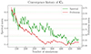 |
Fig. A.1. Convergence history of the covariance. We used the correlation matrix rather than C0 to compute the norms. |
Appendix B: Effective posterior for the initial matter power spectrum when the prior mean differs from the expansion point
We generalise the derivation of the SELFI equations from Leclercq et al. (2019), to the case where the prior mean  differs from the expansion point θ0. The SELFI effective log-likelihood given by Equation (18) can be rewritten in canonical form as
 (B.1)
(B.1)
with  , where we have defined
![Mathematical equation: $$ \begin{aligned} \mathbf N _0&\equiv&\left[ (\nabla \mathbf f _0)^\intercal \mathbf C _0^{-1} \nabla \mathbf f _0 \right]^{-1},\nonumber \\ \mathbf y _0&\equiv&\boldsymbol{\theta }_0 + (\nabla \mathbf f _0)^{-1} \cdot (\boldsymbol{\Phi }_{\rm O}-\mathbf f _0). \end{aligned} $$](/articles/aa/full_html/2025/07/aa53416-24/aa53416-24-eq109.gif) (B.2)
(B.2)
Similarly, the prior given by Equation (7) can be written
 (B.3)
(B.3)
in canonical form, where  . The effective posterior therefore verifies
 (B.4)
(B.4)
where we recognise the canonical form of a Gaussian distribution with covariance matrix
![Mathematical equation: $$ \begin{aligned} \boldsymbol{\Gamma } \equiv \left(\mathbf N _0^{-1} + \mathbf S ^{-1}\right)^{-1}= \left[ (\nabla \mathbf f _0)^\intercal \mathbf C _0^{-1} \nabla \mathbf f _0 + \mathbf S ^{-1} \right]^{-1}, \end{aligned} $$](/articles/aa/full_html/2025/07/aa53416-24/aa53416-24-eq113.gif) (B.5)
(B.5)
and mean
![Mathematical equation: $$ \begin{aligned} \boldsymbol{\gamma }&\equiv&\boldsymbol{\Gamma } (\boldsymbol{\mu }_0+\boldsymbol{\eta }) = \boldsymbol{\Gamma } \left[ (\nabla \mathbf f _0)^\intercal \mathbf C _0^{-1} \nabla \mathbf f _0\boldsymbol{\theta }_0 + (\nabla \mathbf f _0)^\intercal \mathbf C _0^{-1} \nabla \mathbf f _0 (\nabla \mathbf f _0)^{-1}\right. \nonumber \\&\left. \cdot (\boldsymbol{\Phi }_{\rm O}-\mathbf f _0) + \mathbf S ^{-1} \boldsymbol{\hat{\theta }}_{\boldsymbol{\omega }} \right]\nonumber \\&= \boldsymbol{\Gamma } \left\{ \left[(\nabla \mathbf f _0)^\intercal \mathbf C _0^{-1} \nabla \mathbf f _0 + \mathbf S ^{-1}\right] \boldsymbol{\theta }_0 - \mathbf S ^{-1} \boldsymbol{\theta }_0 \right. \nonumber \\&\left. + (\nabla \mathbf f _0)^\intercal \mathbf C _0^{-1} \cdot (\boldsymbol{\Phi }_{\rm O}-\mathbf f _0) + \mathbf S ^{-1} \boldsymbol{\hat{\theta }}_{\boldsymbol{\omega }} \right\} \nonumber \\&= \boldsymbol{\theta }_0 + \boldsymbol{\Gamma } \mathbf S ^{-1} \boldsymbol{\Delta } + \boldsymbol{\Gamma } (\nabla \mathbf f _0)^\intercal \mathbf C _0^{-1} \cdot (\boldsymbol{\Phi }_{\rm O}-\mathbf f _0), \end{aligned} $$](/articles/aa/full_html/2025/07/aa53416-24/aa53416-24-eq114.gif) (B.6)
(B.6)
where  , giving Equation (21).
Appendix C: Consistency checks
C.1. Unbiasedness of the posterior initial power spectrum
To consistently assess the unbiasedness of the method, we sampled ten different ground truth set of cosmological parameters from the prior, computed the corresponding observed vector  for each case, and confirmed both visually and quantitatively that the resulting SELFI posterior remained consistently unbiased. This demonstrates the robustness of the method with respect to the value of the ground truth cosmological parameters.
C.2. Inference using a wiggle-less prior
As a consistency check, we verified that SELFI successfully retrieves the BAOs within the set-up described in this article, even when the prior does not provide any information about the oscillations. We postulate a Gaussian prior given by
 (C.1)
(C.1)
where the expansion point θ0 and the covariance matrix S differ from those of Equation (7). Namely, we set the mean to θ0 ≡ 1ℝS, corresponding to the BBKS power spectrum for the fiducial cosmological parameters, and, following the procedure described by Leclercq et al. (2019), we define the prior covariance matrix as
 (C.2)
(C.2)
where ° denotes the Hadamard product and K is a radial basis function defined by
![Mathematical equation: $$ \begin{aligned} \left(\mathbf K \right)_{ss^{\prime }} \equiv \mathrm{exp} \left[ -\frac{1}{2} \left(\frac{k_s - k_{s^{\prime }}}{k_{\rm corr}}\right)^2 \right], \end{aligned} $$](/articles/aa/full_html/2025/07/aa53416-24/aa53416-24-eq119.gif) (C.3)
(C.3)
and u is a correction accounting for cosmic variance,
 (C.4)
(C.4)
kcorr determines the length scale on which power spectrum amplitudes of different wave number correlate with each other. αcv characterises the “strength” of cosmic variance given the effective volume considered and θnorm2 captures the overall amplitude of the covariance matrix S. The strength of cosmic variance within our simulation volume shall satisfy  at all scales k, where
  is the effective number of modes at scale k, accounting for the window function. As in Leclercq et al. (2019), the hyperparameters kcorr and θnorm are optimised to reproduce the shape of a fiducial wiggle vector θfid, using the effective posterior distribution obtained in Section 2.2.2 as the likelihood; that is,
 (C.5)
(C.5)
where γ and Γ inherit their dependence on kcorr and θnorm through S. We use Gaussian hyperpriors on (kcorr, θnorm), namely kcorr ∼ 𝒢(0.020, 0.0152) [h Mpc−1] and θnorm ∼ 𝒢(0.2, 0.32). We estimated the maximum a posteriori using L-BFGS (Liu & Nocedal 1989) and found  and θnorm = 0.034743, values that were used to obtain the prior on θ corresponding to the shaded yellow area in Figure C.1.
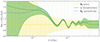 |
Fig. C.1. Wiggle-less prior and corresponding SELFI posterior on the initial matter power spectrum θ. The prior mean θ0, also used as expansion point, is indicated by the yellow line; its 2σ credible region corresponds to the yellow-shaded area. The posterior mean γ and 2σ credible region correspond to the green line and shaded area. The ground truth θgt is indicated by the solid blue line. The dashed red line denotes the Nyquist frequency. Even though the prior contains no information about the BAOs, the SELFI posterior is consistently unbiased across all scales and accurately retrieves the oscillations up to k ≃ 0.2 h/Mpc. |
The posterior obtained with the wiggle-less prior is in green in Figure C.1. It is consistent with the ground truth. Notably, it accurately retrieves the oscillations up to k ≃ 0.2 h/Mpc, even though the prior is completely agnostic to the BAOs, except through its hyperparameter optimisation.
Appendix D: Impact of linear galaxy bias parameters
The linear galaxy bias parameters have a quadratic scale-independent impact on the galaxy overdensity power spectrum. We show qualitatively that this is expected to hold true for the SELFI posterior, to some extent. Indeed, neglecting the term ΓS−1Δ, which we measured to be smaller than 10−3 at all scales in our set-up, the SELFI filter equation (20) for the mean of the posterior on the matter power spectrum can be rewritten:
 (D.1)
(D.1)
If we consider for simplicity the case where the overall noise level is σ = 0, for a fixed phase, Pgi(kr) becomes a deterministic function of bgi given by
where  denotes the discrete Fourier transform of h. Hence, in the absence of noise, a constant relative error on all the three squared linear galaxy biases has a scale-independent impact on any simulated summary Φ obtained with the hidden-box simulator. By linearity of the 𝔼 and ∂θ operators, the relative impacts on f0 and ∇θf0 are scale-independent as well and quadratic in bgi. Similarly, from Equation (13), C0−1 scales as bgi−4, so that, from Equation (21), Γ and therefore Γ (∇θf0)⊺ C0−1f0 are left unaffected and only the
  term in Equation (D.1) is impacted by misspecified galaxy biases. If the misspecified biases are such that the relative error (bimis)2/bgi2 = ϵ is independent of the population gi, then every component of the vector
  is affected by a factor ϵ, and the overall effect inherits its scale-dependence solely through the covariance matrix Γ. This is the behaviour observed on Figure 9a, where, for a misspecified bias, all the scales undergo about the same shift in number of standard deviations.
Appendix E: Implicit likelihood inference of cosmological parameters
E.1. Numerical set-up
For the ILI of cosmological parameters, we used the variant of ABC-PMC from Simola et al. (2021) implemented in the ELFI package (https://github.com/elfi-dev/elfi, Lintusaari et al. 2018), with minor technical modifications which do not affect the statistical method.
E.2. Population Monte Carlo hyperparameters
The Population Monte Carlo algorithm automatically selects a tolerance sequence based on the procedure described by Simola et al. (2021). It is not completely ϵ-free as one must choose a stopping rule and an initial acceptance threshold for the rejection sampler, the choice of the latter being crucial to prevent the algorithm from getting stuck in local overdense regions of the parameter space. In this study, we set the initial quantile used to determine the corresponding acceptance threshold for the rejection sampling stage to q0 = 0.2.
All Tables
Main variables, their generic role in the statistical framework, and their physical interpretation in this study.
All Figures
|
Fig. 1. Hierarchical representation of the Bayesian framework employed for diagnosing model misspecification and inferring the target parameters ω. The rounded green boxes denote probability distributions, whilst the purple squares represent deterministic functions. 𝒫(ω) is the prior on ω. 𝒯 is a deterministic function linking ω to θ. 𝒫(Φ|θ) denotes the probabilistic data model that maps the space of latent vectors θ to the survey space. The final layer, |
| In the text | |
|
Fig. 2. Detailed representation of the BHM used in this study for the inference of cosmological parameters ω from galaxy surveys. The hidden-box model corresponds to the second dashed orange rectangle and defines the true (unknown) likelihood L(θ) when Φ = ΦO. The variables are ω (the target cosmological parameters), θ (the initial matter power spectrum), ψ (the nuisance parameters), o (the cosmological parameters, formally treated as nuisance parameters within the hidden-box), d (the full data vector containing the full galaxy count fields), Φ (the summary statistics), and |
| In the text | |
|
Fig. 3. Illustration of the galaxy survey data model used in this study. (Upper and middle rows) Slices through a realisation of the dark matter overdensity fields in real space (top) and redshift space (middle). The fields are evolved in time using N-body simulations, starting from a grid of Gaussian initial dark matter density fluctuations with power spectrum θgt, up to the redshift indicated above the corresponding panels. (Lower row) Observed galaxy number count fields for the three galaxy populations, each defined on a grid of 5123 cells. Light-cone effects are accounted for by using one effective redshift per galaxy population. Each slice passes through the observer located at the (0, 0, 0) corner of the box. |
| In the text | |
|
Fig. 4. Radial selection functions modelled as log-normal distributions in redshift (upper x axis) for the three mock galaxy populations. In the figure, the distributions are represented with respect to comoving distances (lower x axis) using the redshift-distance relation. The continuous lines represent the selection functions for the well-specified Model A, while the dotted lines represent the misspecified Model B, both defined by the values provided in Table 4. The small, percent-order difference between Models A and B renders the dotted curves nearly indistinguishable from the solid ones. The vertical dashed lines indicate the means of the log-normal distributions. |
| In the text | |
|
Fig. 5. Survey mask for the well-specified Model A. We added extinction linearly decreasing from 100% at the galactic plane to 0% at 60° galactic latitude (dash-dotted orchid line), along with 256 holes of approximately 0.1-degree radius (white crosses). The observed octant is delineated by the light orchid triangle. The colour scale represents the completeness function |
| In the text | |
|
Fig. 6. Data intervening in the computation of the SELFI posterior. (Left panels) Observed and simulated summary statistics for Model A (well-specified; upper panel) and B (misspecified; lower panel). For each population, the simulated summaries are shown in grey and their means are represented as dotted coloured lines. The shaded areas correspond to ±2σ around their mean. The solid black line corresponds to the observations ΦO. The binning is indicated by the vertical dashed lines. Right panels: covariance matrices for Models A and B. For each (k, k′) entry, the colour scale represents the covariance between the k-th and k′-th modes. The diagonal blocs of the full covariance matrix correspond to the intra-population covariance; the extra-diagonal blocs correspond to the inter-populations covariances. |
| In the text | |
|
Fig. 7. Prior and SELFI posteriors for the initial matter power spectrum θ given the observations ΦO. The ground truth θgt is indicated by the dashed blue line. The prior and posterior means, θ0, γA and γB, are represented respectively by the yellow, green and red lines, along with their 2σ credible regions (shaded yellow, green, and red areas). The vertical dashed lines indicate the support wave numbers for the initial matter power spectrum representation. The posterior obtained with the well-specified Model A is unbiased over all scales, whilst the posterior obtained with the misspecified Model B exhibits an excess and a lack of power at the largest and smallest scales, respectively. |
| In the text | |
|
Fig. 8. Histogram of the Mahalanobis distances dM(θn, θ0|S) between the prior and 5000 power spectra θn ≡ 𝒯(ωn) sampled from Equation (6). The mean value is indicated by the vertical solid black line. The green and red lines indicate the distances from γA and γB to the prior, respectively. |
| In the text | |
|
Fig. 9. Ensemble of SELFI posteriors for the initial matter power spectrum θ conditional on the observed data ΦO for different observational models, used to diagnose systematic effects. All the posteriors are derived from a single, common set of N-body simulations. They make it possible to disentangle individual systematic contributions by comparing their differential impact across the range of wave numbers spanned by the power spectra. The colour scales indicate the relative error associated with the systematic effects considered in each sub-figure. The solid yellow line denotes the prior mean θ0 and the ground truth θgt is indicated by the dashed blue line. The vertical dashed lines indicate the support wave numbers for the initial matter power spectrum representation. The 2σ credible regions for the prior and the posterior with the well-specified Model A correspond to the shaded yellow and green areas, respectively. The posterior means γ are represented by the coloured continuous lines for varying degrees of misspecification. For clarity, their corresponding credible regions have been omitted. (a) Impact of misspecified linear galaxy biases. (b) Impact of misspecified linear extinction. (c) Impact of misspecified redshifts. (d) Impact of misspecified selection function variances. (e) Impact of misspecified number of holes. (f) Impact of misspecified selection function variances (varying) under misspecified linear extinction (fixed). |
| In the text | |
|
Fig. 10. Profiles of the well- and misspecified selection functions Ri for the three mock galaxy populations. The continuous lines represent the selection functions used in Model A. The dashed lines are derived by underestimating n1, 2(z) by 10% whilst maintaining ntot(z) constant. |
| In the text | |
|
Fig. 11. Impact of the gravity solver parameters on the SELFI posterior. Panels (a, c, e) display the summary statistics Φ for the three galaxy count fields, comparing the well-specified Model A (dashed lines) with the misspecified model (solid lines). The lower parts of these panels show the relative error between the two models, with shaded regions corresponding to a 1% error margin. Panels (b, d, f) show the corresponding SELFI posteriors for the initial matter power spectrum θ, with the well-specified and misspecified models represented by green and indigo lines, respectively. (a) Example of summary statistics for a single realisation with nsteps = 10 (solid lines) as opposed to nsteps = 20 time steps for Model A (dashed lines) in the gravitational evolution with COLA. Although the direct error remains well below 1% across all scales, the inverse error on the SELFI posterior (b) reaches 2% at the largest scales, corresponding to a deviation greater than 1σ from the well-specified Model A. (c) Summary statistics using only the final snapshot at redshift z1 = 0.15 for the three mock galaxy populations, thereby neglecting light cone effects (solid lines). The forward error reaches 74% at the largest scales for the most distant galaxy population, and the corresponding SELFI posterior (d) significantly rejects the ground truth across all scales. (e) Summary statistics using a pure 2LPT gravity model instead of N-body simulations to define the galaxy populations (solid lines). The forward error reaches ∼7% at the smallest scale, and the ground truth is significantly rejected by the SELFI posterior (f), which deviates by more than 2σ compared to Model A at the largest scales. |
| In the text | |
|
Fig. 12. Prior 𝒫(ω) (yellow) and posterior |
| In the text | |
|
Fig. A.1. Convergence history of the covariance. We used the correlation matrix rather than C0 to compute the norms. |
| In the text | |
|
Fig. C.1. Wiggle-less prior and corresponding SELFI posterior on the initial matter power spectrum θ. The prior mean θ0, also used as expansion point, is indicated by the yellow line; its 2σ credible region corresponds to the yellow-shaded area. The posterior mean γ and 2σ credible region correspond to the green line and shaded area. The ground truth θgt is indicated by the solid blue line. The dashed red line denotes the Nyquist frequency. Even though the prior contains no information about the BAOs, the SELFI posterior is consistently unbiased across all scales and accurately retrieves the oscillations up to k ≃ 0.2 h/Mpc. |
| In the text | |
Current usage metrics show cumulative count of Article Views (full-text article views including HTML views, PDF and ePub downloads, according to the available data) and Abstracts Views on Vision4Press platform.
Data correspond to usage on the plateform after 2015. The current usage metrics is available 48-96 hours after online publication and is updated daily on week days.
Initial download of the metrics may take a while.