| Issue |
A&A
Volume 698, June 2025
|
|
|---|---|---|
| Article Number | A317 | |
| Number of page(s) | 20 | |
| Section | Extragalactic astronomy | |
| DOI | https://doi.org/10.1051/0004-6361/202553943 | |
| Published online | 23 June 2025 | |
Possible environmental quenching in an interacting little red dot pair at z ∼ 7
1
Institute for Computational Astrophysics and Department of Astronomy and Physics, Saint Mary’s University, 923 Robie Street, Halifax, NS B3H 3C3, Canada
2
Observatorio Astronómico de Córdoba, Universidad Nacional de Córdoba, Laprida 854, X5000 Córdoba, Argentina
3
Department of Astronomy, Kyoto University, Sakyo-ku, Kyoto 606-8502, Japan
4
Kapteyn Astronomical Institute, University of Groningen, P.O. Box 800, 9700AV Groningen, The Netherlands
5
Faculty of Mathematics and Physics, Jadranska ulica 19, SI-1000 Ljubljana, Slovenia
6
David A. Dunlap Department of Astronomy and Astrophysics, University of Toronto, 50 St. George Street, Toronto, Ontario M5S 3H4, Canada
7
INAF – Osservatorio Astronomico di Roma, Via Frascati 33, Monte Porzio Catone 00078, Italy
8
National Research Council of Canada, Herzberg Astronomy & Astrophysics Research Centre, 5071 West Saanich Road, Victoria, BC V9E 2E7, Canada
9
Department of Physics and Astronomy, University of California Davis, 1 Shields Avenue, Davis, CA 95616, USA
10
Cosmic Dawn Center (DAWN), Copenhagen, Denmark
11
Niels Bohr Institute, University of Copenhagen, Jagtvej 128, DK-2200 Copenhagen N, Denmark
12
Columbia Astrophysics Laboratory, Columbia University, 550 West 120th Street, New York, NY 10027, USA
13
Department of Physics and Astronomy, York University, 4700 Keele St. Toronto, Ontario M3J 1P3, Canada
14
Space Telescope Science Institute, 3700 San Martin Drive, Baltimore, Maryland 21218, USA
⋆ Corresponding author: This email address is being protected from spambots. You need JavaScript enabled to view it.
Received:
28
January
2025
Accepted:
14
May
2025
Abstract
We report the discovery of a z ∼ 7 group of galaxies that contains two little red dots (LRDs) just 3.3 kpc apart, along with three potential satellite galaxies, as part of the Canadian NIRISS Unbiased Cluster Survey (CANUCS). The spectral energy distributions (SEDs) of this LRD pair show evidence of a Balmer break, consistent with a recent (∼100 Myr) quenching of star formation. In contrast, the satellites are compatible with a recent-onset (∼100 Myr), ongoing burst of star formation. LRD1’s SED is consistent with a dust-free active galactic nucleus (AGN) being the source of the UV excess in the galaxy. The optical continuum would be powered by the emission from an obscured post-starburst and the AGN at a subdominant level. LRD2’s SED is more ambiguous, but it could also be indicative of a dust-free AGN. In this scenario, these LRDs would be massive (M⋆ ∼ 1010 M⊙) and dusty (A(V) > 1 mag) and the three satellites would be lower-mass objects (M⋆ ∼ 108 − 9 M⊙) subject to low dust attenuations. The proximity of the two LRDs suggests that their interaction is responsible for their recent star formation histories, which can be interpreted as environmental bursting and quenching in the epoch of reionization.
Key words: galaxies: active / galaxies: evolution / galaxies: high-redshift / galaxies: interactions
© The Authors 2025
 Open Access article, published by EDP Sciences, under the terms of the Creative Commons Attribution License (https://creativecommons.org/licenses/by/4.0), which permits unrestricted use, distribution, and reproduction in any medium, provided the original work is properly cited.
This article is published in open access under the Subscribe to Open model. This email address is being protected from spambots. You need JavaScript enabled to view it. to support open access publication.
1. Introduction
Little red dots (LRDs; Labbé et al. 2023; Barro et al. 2024; Greene et al. 2024; Matthee et al. 2024) represent one of the most remarkable discoveries made by the JWST (Gardner et al. 2023). These red, compact sources show a characteristic V-shaped spectral energy distribution (SED) consisting of a nearly flat to blue rest-frame ultraviolet (UV) continuum and a very steep slope in the optical. These properties make LRDs a challenge for SED modeling, even with the aid of spectroscopic data.
As summarized in Pérez-González et al. (2024), there are different potential explanations for LRDs, including high equivalent width (1000 Å) emission lines that boost the broadband photometry (e.g., Yuma et al. 2010; Pérez-González et al. 2023; Desprez et al. 2024; Hainline et al. 2025); a flexible treatment of the dust attenuation (e.g., Akins et al. 2023; Barro et al. 2024; Li et al. 2025); active galactic nuclei (AGNs; e.g., Inayoshi & Maiolino 2025; Li et al. 2025); and hybrid models that combine AGNs and stars (e.g., Kocevski et al. 2023; Greene et al. 2024; Kokorev et al. 2024; Tripodi et al. 2024; Wang et al. 2024). However, none of these approaches has been able to fully reproduce the SEDs of the bulk of the LRD population.
Little red dots are generally X-ray-weak (Ananna et al. 2024; Maiolino et al. 2025), mostly radio-quiet (Labbé et al. 2023; Perger et al. 2025), and remain undetected in the (sub)millimeter range (Casey et al. 2024; Labbe et al. 2025). They do not show signs of variability (Zhang et al. 2025), and their mid-infrared SED is more consistent with emission from stars (Pérez-González et al. 2024; Williams et al. 2024). On the other hand, > 50% of the photometrically selected LRDs display broad Balmer and/or Paschen lines (e.g., Kocevski et al. 2023; Greene et al. 2024; Tripodi et al. 2024). The prevailing view is that the SEDs of these galaxies are not solely driven by an AGN, but rather have a hybrid origin.
The formation and evolution of these galaxies is also uncertain. They have been proposed to both be the progenitors of the first massive galaxies (e.g., Setton et al. 2024; Tripodi et al. 2024; Wang et al. 2024) and low-mass objects hosting an AGN (Chen et al. 2025). Most LRDs are found isolated in the field, yet JWST studies reveal a mean number of merger events per galaxy of ∼4 Gyr−1 at 6.5 < z < 7.5 (Duan et al. 2025). Tanaka et al. (2024) reported three of the first dual LRD candidates, with projected separations of 0.2–0.4″, in the COSMOS-Web survey (Casey et al. 2023). Interactions could thus play a major role in the triggering of potential AGN activity and quenching in LRDs (see also Greene et al. 2024; Labbe et al. 2024).
We explore the impact of the environment on LRDs, presenting a dual LRD candidate at z ∼ 7 that could be undergoing merging, bursting, and quenching events. The pair is likely embedded in a galaxy group that has three satellite galaxies and shows signs of coordinated star formation histories (SFHs).
Throughout this work we assume ΩM, 0 = 0.3, ΩΛ, 0 = 0.7, and H0 = 70 km s−1 Mpc−1 and use AB magnitudes (Oke & Gunn 1983). All stellar mass (M⋆) and star formation rate (SFR) estimates assume a Chabrier (2003) initial mass function (IMF).
2. Data
We used data from the Canadian NIRISS Unbiased Cluster Survey (CANUCS; GTO program #1208; Willott et al. 2022), which consists of Near Infrared Camera (NIRCam; Rieke et al. 2023) and JWST Near InfraRed Imager and Slitless Spectrograph (NIRISS; Doyon et al. 2023) observations of five strong lensing clusters and flanking fields. CANUCS also incorporates Near Infrared Spectrograph (NIRSpec; Jakobsen et al. 2022) PRISM spectroscopy in these fields.
Our objects are located behind the z = 0.375 cluster Abell 370 and were observed with the NIRCam F090W, F115W, F150W, F200W, F277W, F356W, F410M, and F444W filters for 6.4 ks each, reaching 3σ point source limiting magnitudes ranging from 29.5 to 30.2 mag. Archival Hubble Space Telescope (HST) imaging from the Advanced Camera for Surveys (ACS; namely, F606W and F814W) in this field were also included (HST-GO-15117 PI Steinhardt; Steinhardt et al. 2020). The 3σ point source limiting magnitudes, based on the uncertainty of nearby detections, reach ∼27.4 − 28.0 mag for these ACS images. Spectroscopy from NIRISS or NIRSpec is not available for these objects.
The CANUCS and archival images were processed and bright cluster galaxies were removed as described in Noirot et al. (2023) and Martis et al. (2024). Their point spread functions (PSFs) were then degraded to match that of the F444W image (Sarrouh et al. 2024), after which photometry was done in matched apertures magnitudes (Asada et al. 2024); for some of the galaxies targeted in this paper, we also performed point-source photometry (see Sect. 3.2). Photometric redshifts for all detected sources were measured with EAzY (Brammer et al. 2008) using the standard templates augmented with the Larson et al. (2023) set (see Asada et al. 2025 for more details). We used the intergalactic medium (IGM) attenuation curve of Asada et al. (2025), which has been shown to greatly reduce photo-z systematics at z > 6 by accounting for the effect of the Lyα damping wing from the circumgalactic medium (CGM) gas.
3. The z ∼ 7 group
3.1. Discovery and basic properties
Examining the CANUCS catalogs, we find a potential close group of four 6.79 < zphot < 6.87 objects (z ∼ 7.0 using the Inoue et al. 2014 standard IGM transmission in the case of the LRDs); see Fig. 1.
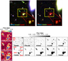 |
Fig. 1. Cutouts of the galaxy group in different bands. (1): 8 × 8 arcsec2 cutouts of two RGB images based on F277W, F410M, and F444W (left) and F150W, F200W, and F444W (right) NIRCam imaging. The yellow square encloses the region that contains our galaxies; its dimensions are 2.8 × 2.4 arcsec2. These images highlight the common F410M excess (and thus the high-z nature) in this galaxy group compared to sources in the neighborhood (left) and the more prominent emission in F444W of the LRD pair compared to the satellites (right). The red squares in both panels show a zoomed-in view of the LRD pair in a less saturated scale to highlight the difference in color between the LRDs and SAT0. The arrow in the left panel points to a z ∼ 7 source ∼18 kpc away from the LRD pair, with colors similar to the satellite galaxies. (2): Cutouts of our galaxy group in smoothed versions of F200W, F277W, and F410M obtained using a Gaussian filter with σ = 1.2 pixels. (3): Postage stamps of these sources in the different HST and NIRCam bands at native spatial resolution. NIRCam images are plotted following the same scale as above. For the HST bands, the upper limit was set to 3 nJy to deal with the noise. The kiloparsec scale is not corrected for lensing magnification, which is also low at this position and redshift (μ = 1.26; see Fig. A.1). |
In addition to the setting described in the previous section, we ran EAzY using the template model built from the J0647_1045 LRD at z = 4.53 from Killi et al. (2024). This galaxy was well fitted assuming that the optical/near-infrared emission and the broadband lines are generated from a relatively massive AGN while the less obscured UV continuum and narrow lines are produced, at least partly, by a small but spatially resolved star-forming host galaxy. The photo-zs found for the LRD pair are then 7.01 and 7.00, respectively.
With  , the redshifts of all these galaxies are indistinguishable given our photo-z uncertainties (Asada et al. 2024, 2025). The photo-zs are well constrained by excess flux in the F410M medium band (due to redshifted Hβ and [OIII]λλ4959, 5007 emission lines), a red F277W − F356W color (due to either the Balmer break or strong emission lines at λrest > 4000 Å), and a sharp drop across F090W − F115W (due to the Lyman Break at rest-1215 Å).
Visual inspection of the short wavelength bands reveals that the brightest source consists of two distinct components – dubbed CANUCS-A370-LRD1 and CANUCS-A370-SAT0 (LRD1 and SAT0 for short; see the F200W panel of Fig. 1, including the labels), blended in the CANUCS catalog. Using SExtractor (Bertin & Arnouts 1996) on the original (unsmoothed) F150W image, we recovered the centroids of the five objects in the group: CANUCS-A370-LRD1, -SAT0, -LRD2, -SAT1, and -SAT2. SAT1 fragments into three subcomponents: SAT1a, SAT1b, and SAT1c (see Fig. B.1), although we treated it as a single galaxy here.
We built a custom local lens model based on Gledhill et al. (2024), incorporating information from three foreground galaxies close to the line of sight of our LRD system and using a new galaxy-galaxy lens that we discovered in one of these foreground sources (see Appendix A for further details). Our new lensing model yields a magnification of  at the position of the LRD pair. We verified the result by replacing the external shear with the best cluster lens model from Gledhill et al. (2024). The result (
 ) is consistent with our simplified model. The positions of our galaxies corrected for lensing are reported in Table A.1.
The five sources form a potential close group; the two brightest sources, LRD1 and LRD2, are at a projected distance (corrected for magnification and considering a scale of 5.4 kpc/arcsec) of only 3.27 kpc; LRD1 and SAT0 are separated by just 0.97 kpc; and LRD1 is separated from SAT1 and SAT2 by 6.35 kpc and 6.90 kpc, respectively. Additionally, there is evidence of a tidal structure or an outflow connecting LRD1 to SAT2, as highlighted by the F277W and F410M smoothed maps in Fig. 1. At these z, these bands would be probing potential [OII]λλ3726, 3729 and [OIII]λλ4959, 5007 emission, respectively. The proximity of the objects in redshift and on the sky, as well as the hints of a physical connection between LRD1 and SAT2, are the first indications of the possible interacting nature of this galaxy group.
As also highlighted in Fig. 1, there is another source to the north of our galaxy group (a possible SAT3) whose F410M excess is indicative of z ∼ 7, compatible with the colors displayed by our satellite galaxies. It has a magnification  and is located ∼18 kpc away from the LRDs (corrected for lensing), and thus its physical connection to the galaxy group can be questioned. We report the photometry and physical properties of this source in Appendix C.
3.2. Revised photometry and LRD identification
Given how close LRD1, LRD2, and SAT0 are, and the compactness of these objects, we went beyond the aperture photometry of Sect. 2 and performed PSF photometry for these three sources. We retained the aperture photometry from the catalogs measured in 0.5″ and 0.3″ apertures for SAT1 and SAT2, respectively. Details regarding our measurements are included in Appendix B, and Table B.1 reports the flux measurements for each source. Using the updated photometry, we recomputed photo-zs, arriving at the values listed in Table F.1.
To identify possible LRDs, we used the criteria for high-z sources from Kokorev et al. (2024) and the criteria from Kocevski et al. (2024). These and other LRD criteria are based on computing a set of colors along the SED, imposing a blue rest-frame UV continuum and a red optical continuum. They also include a compactness criterion and a screening for brown dwarfs. According to Kokorev et al. (2024):
 (1)
(1)
 (2)
(2)
 (3)
(3)
 (4)
(4)
 (5)
(5)
In this case, we used the fluxes measured within 0.3 and 0.5″ apertures based on the PSF-matched images to compute the compactness. The color criteria were calculated using the PSF photometric values. According to Kocevski et al. (2024):
 (6)
(6)
 (7)
(7)
 (8)
(8)
 (9)
(9)
 (10)
(10)
 (11)
(11)
where rh stands for the half-light radius as measured in the F444W band, rh, stars denotes the stellar locus (as defined in their Fig. 4), S/N is the signal-to-noise ratio, and
To determine βopt and βopt, we used the magnitudes measured in bands blueward and redward of 3645 Å based on the z of our galaxies, again corresponding to PSF photometry. The half-light radii were computed based on a Gaussian fit from the RadialProfile photutils method (Bradley 2023). In Table 1 we include the values for the different criteria retrieved for the LRD pair and SAT0, as well as the compactness measured in every photometric band.
Values for the criteria established in Kokorev et al. (2024) and Kocevski et al. (2024), defined in Sect. 3.2, obtained for the LRD pair and SAT0.
LRD1 and LRD2 pass these screenings, while SAT0 satisfies most of the color criteria but its LRD nature is more uncertain as its proximity to LRD1 involves a certain contamination, even for the PSF photometry. This contamination also makes it difficult to check its compactness. In addition, as highlighted by the red-green-blue (RGB) images in Fig. 1, SAT0 shows different colors from those displayed by the LRDs, more compatible with SAT1 and SAT2. We cannot make any further conclusions about the nature of this object with our data and will treat it as a satellite source.
LRD1 reaches ∼25 mag in the rest-frame optical and ∼27 mag in the UV, which places it among the brightest LRDs known in the legacy fields from Kocevski et al. (2024). LRD2 is fainter, reaching ∼26 mag in the optical and ∼28 mag in the UV, comparable to typical LRDs. The satellites are also fainter, and SAT0 is the brightest among them. It reaches ∼25.5 − 26.5 mag in the optical and 27 mag in the UV. SAT1 and SAT2 display average values of 28 and 28.5 mag, respectively.
4. SED fitting
We fitted the photometry of LRD1, LRD2, and the satellites using Dense Basis (Iyer & Gawiser 2017; Iyer et al. 2019) and Bagpipes (Carnall et al. 2018). One of the primary advantages of Dense Basis is that it utilizes nonparametric SFHs, which work better than parametric models capturing the variety of physical events (e.g., bursts, rejuvenation, sudden quenching, or maximally old star formation) that shape the complex SFHs of high-z galaxies (Simha et al. 2014; Leja et al. 2019). Stellar population synthesis models are incorporated into the code through the Flexible Stellar Population Synthesis (FSPS; Conroy & Gunn 2010) Python module. It allows for the inclusion of the infrared emission of an AGN’s dusty torus based on the Nenkova et al. (2008) templates, but the emission from the accretion disk in the UV-to-optical is not considered. Consequently, Dense Basis can only be effectively used to fit the emission due to stars at these wavelengths.
On the other hand, Bagpipes allows the UV and optical emission due to an AGN accretion disk to be modeled using a double power-law model. A parameterization for the SFH is normally selected in this code, although the code also allows for nonparametric SFHs in a different way than Dense Basis. It uses a series of piecewise constant functions in lookback time, requiring a number of bins, a prior distribution, and an alpha parameter that controls the correlation between the tx (the age at which the galaxy formed x% of its M⋆) and the SFH (Leja et al. 2019). Dense Basis does not require these time bins and we can choose a set of custom values of alpha for each parameter.
We opted to use the Dense Basis code to fit the stellar emission and recover the SFHs of these galaxies and explored the AGN scenario using Bagpipes, and a combination of the two codes. More details regarding the Dense Basis and Bagpipes methods and configurations can be found in Appendices D and E, respectively. The physical parameters obtained for each source are reported in Table F.1.
The interplay between the peak of the Lyα emission and the damping wing absorption plays a significant role at this redshift, as mentioned in Sect. 2. Since Dense Basis and Bagpipes use the default IGM attenuation curve, and the attenuation is in any case stochastic, we did not consider filters close to this feature in the SED fitting, namely F814W, F090W, and F115W. Our effective photometry comprises six filters (five broad bands and one medium band) spanning from F150W to F444W. We are aware that our data are highly susceptible to overfitting and thus results are highly model-dependent. However, this study aims to provide just initial insights into the nature of these objects and their SFHs.
When using a broad prior for the redshift in these codes, both Dense Basis and Bagpipes favor a z ∼ 7 solution for the LRD pair (using the six filters mentioned above, not considering the filters close to the Lyα damping wing). These results are in line with the photo-zs reported by EAzY when using the Killi et al. (2024) template. However, the models used by SED fitting codes such as Dense Basis and Bagpipes still need to be fine-tuned to account for the physical conditions ruling at these early epochs. Furthermore, LRDs are very peculiar objects that currently present a challenge to SED fitting codes. Considering that the satellites’ photo-zs are less uncertain since these are normal star-forming galaxies (SFGs), we can use these values as the redshift of the galaxy group (i.e., z ∼ 6.8). To do so, we restricted the redshift prior to 6.75 < z < 6.85 in Dense Basis and Bagpipes.
In addition, given the available data and the limitations and biases of our SED fitting codes, we opted to be cautious and explored a more conservative approach, considering small variations to this prior. These variations also account for the possibility that the LRDs and the satellites were not located at the same z, as well as the random IGM and/or CGM attenuation variations along the line of sight, which could potentially lead to small variations in our galaxies’ photo-zs. To deal with this, we added two more redshift ranges, restricting the priors to 6.75 < z < 6.95 (allowing for a slightly higher redshift), and 6.95 < z < 7.15 (to explore the z ∼ 7 case). We refer to these intervals as the low- (6.75 < z < 6.85), mid- (6.75 < z < 6.95), and high-z (6.95 < z < 7.15) cases hereafter, recalling that the low-z interval is the one centered around the actual photo-z of this potential galaxy group.
4.1. Stellar fits from Dense Basis
We assumed wide ranges for the priors of the stellar mass and SFR, constraining the M⋆ between 7 < log M⋆/M⊙ < 12 and the SFR between −1 < log SFR [M⊙/yr]< 3, and setting a flat specific SFR. For parameters such as dust attenuations or metallicities, the default Dense Basis configuration was used, which considers a Calzetti et al. (2000) dust attenuation law. Additional details regarding our setting can be found in Appendix D.
The left panel in the first row of Fig. 2 shows the stellar best-fitting models from Dense Basis for LRD1. These models correspond to a dusty (A(V) ∼1.0 − 1.2 mag) and massive (M⋆ ∼ 1010.4 − 10.5 M⊙) Balmer break galaxy. Residuals show that the solutions that best fit the F150W and F200W points (e.g., the low- and mid-z cases, with < 25% residuals) deviate more from the F277W point (> 75%). LRD1 is thus poorly fitted using only stars, especially in the rest-frame UV, where the code cannot well reproduce the flat slope and provides a steeper model with a high A(V) (see Appendix D for more details on priors and tests). All these factors indicate a potential additional component, responsible for the UV flux excess.
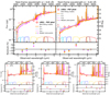 |
Fig. 2. (a): Dense Basis stellar fits based on the LRD1 (left) and LRD2 (right) PSF photometry (red open circles). Data points excluded from the fits are shown using thinner lines. Solid orange, blue, and fuchsia lines depict the fits for the low- (thicker line, corresponding to the photo-z of the galaxy group), mid-, and high-z intervals. The corresponding model photometric points are shown with filled circles. (b): Dense Basis stellar fits for the satellite galaxies based on PSF (SAT0) and aperture (SAT1, SAT2) photometry, following the same color code as above. We include the HST and NIRCam transmission curves, as well as the residuals of the fits. |
LRD2’s stellar fit is displayed in the right panel, first row, of Fig. 2. All of the solutions indicate a massive (M⋆ ∼ 109.7 − 9.8 M⊙) Balmer break galaxy, subject to an uncertain degree of attenuation (A(V) ∼ 0.62 − 1.26 mag). Residuals highlight the difficulty of fitting the break as defined by the F277W point while accounting for the UV flux. However, the high-z case seems to provide a better balance between the two tasks, fitting the UV and the break with residuals ≲25% in F150W and ∼50% in F277W, suggesting a potential stellar origin for this source.
Previous studies have also found Balmer break LRDs spanning M⋆ ∼ 109 − 11 M⊙ (see Gentile et al. 2024 at z = 5.051 and 6.7; Ma et al. 2025 at z = 7.04; Wang et al. 2024 at 6.7 < z < 8.4; Williams et al. 2024 at 5.5 < z < 7.7; Labbe et al. 2024 at z = 4.47). In fact, Wang et al. (2024) provide a sample of spectroscopically confirmed Balmer break LRDs at the same zspec of our sources, suggesting that such Balmer breaks are possible in LRDs at this epoch. The number of reported LRDs with a Balmer break is probably too low as some might have been discarded in works whose screenings excluded galaxies that show strong emission lines and/or strong breaks to ensure a rising red continuum (e.g., Labbé et al. 2023; Greene et al. 2024; Kocevski et al. 2024; Kokorev et al. 2024).
However, it is also important to remember that emission lines can mimic Balmer breaks, which would lead to overestimated values of M⋆ (Desprez et al. 2024), as in a fraction of objects from Labbé et al. (2023). Labbé et al. (2023) was based on the analysis of NIRCam broad-band photometry, while we benefit from an emission excess in a medium-band filter, F410M, likely produced by [OIII]λλ4959, 5007 + Hβ, which also allows us to better constrain the photo-zs of our galaxies. Still, we cannot rule out the possibility that these breaks are partially or totally induced by emission lines. Further spectroscopic confirmation of this feature is required. Additional discussion regarding potential contamination due to emission lines can be found in Appendix D.
Panels in the second row in Fig. 2 depict the stellar fits for the satellites. SAT0 is potentially a SFG. It can also be fitted with a Balmer break at z ∼ 7, although the colors of this source according to Fig. 1 favor the SFG scenario. All the fits suggest a massive object subject to a low dust obscuration, with M⋆ ∼ 109.2 − 9.4 M⊙ and A(V) ∼ 0.1 − 0.3 mag. SAT1 and SAT2 are lower-mass ∼ 108.0 M⊙ SFGs with low attenuations (A(V) < 0.3 mag) at the three redshift intervals. Residuals for SAT1 and SAT2 are small, ≲20%, highlighting that the source of the high residuals in the LRD fits is not our methodology but rather the unusual nature of these targets.
4.2. AGN modeling with Bagpipes
The results obtained with Dense Basis for the LRDs, especially LRD1, point to a UV excess that cannot be fitted only with stars with current models. Several recent works suggest that this emission could result from extremely low dust attenuation conditions in which dust is not destroyed but pushed out by kiloparsec-scale outflows (the attenuation-free model; Ferrara et al. 2023; Ziparo et al. 2023; Ferrara 2024a, 2024b). A top-heavy IMF (Trinca et al. 2024; Hutter et al. 2025), a higher star formation efficiency (Dekel et al. 2023; Li et al. 2024), or star formation variability (Mirocha & Furlanetto 2023; Pallottini & Ferrara 2023) are also being explored as possible drivers of these blue colors. On the other hand, this emission could be powered by a nonstellar source, such as an AGN. In this section we explore this last possibility using Bagpipes (see also Appendix E), keeping in mind that this is just only one of the different potential scenarios that could explain this excess in our LRDs.
We fitted the photometric points of the two LRDs using a composite model consisting of a stellar population plus an AGN employing the Multinest sampling algorithm. In the case of LRD1, Bagpipes chooses a z ∼ 7 solution, as previously mentioned. For the low-z prior (the photo-z of the galaxy group, z ∼ 6.8), the fit does not converge, probably due to limits in the code (see Sect. 4). We explored the other two redshift cases to provide some hints about the possible AGN nature of this LRD.
The best-fitting model from Bagpipes (stars + AGN) for LRD1 (z ∼ 7) is presented in Fig. 3. Its isolated AGN photometric component is shown in the top panel of Fig. 4. The AGN continuum is modeled by an unobscured broken power-law dominating the UV, which has been found to reproduce well the average observed Sloan Digital Sky Survey (SDSS) quasar spectra (e.g., Vanden Berk et al. 2001; Temple et al. 2021). This model has also been proposed for LRDs at high-z (e.g., Kocevski et al. 2023; Tripodi et al. 2024; Zhang et al. 2025). On the other hand, a broad Hβ emission line and a reddened stellar population dominate the optical SED.
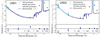 |
Fig. 3. Bagpipes best fits (stars + AGN) for LRD1 (left) and LRD2 (right) based on PSF photometry (red open circles), corresponding to the high-z solution obtained using a broad z prior. Cyan circles depict the synthetic photometric points associated with the best-fitting model, shown as a thick blue line (50th percentile). The limits of the shaded blue region represent the 16th and 84th percentiles. The residuals for the models, corresponding to the 16th (squares), 50th (diamonds), and 84th (circles) percentiles, are also included underneath each panel. |
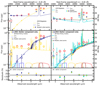 |
Fig. 4. Top panels: Potential AGN fits (dashed cyan for the low-z, yellow for the mid-z, navy for the high-z cases) for LRD1 (left) and LRD2 (right) derived using Bagpipes (Sect. 4.2). The low-z case is not represented in the LRD1 panel (left) because it did not converge in Bagpipes. Crosses depict their photometric points. Middle panels: Dense Basis fits for the stellar component of LRD1 (left) and LRD2 (right) obtained by subtracting the AGN photometry derived with Bagpipes from the PSF photometry (Sect. 4.3). The LRD PSF photometry is shown as red open circles. Photometric points from the stellar component are shown as cyan, yellow, and navy open circles for the low-, mid-, and high-z cases, respectively. Best-fit models are displayed as solid lines in the same color. The low-z case (thicker line) corresponds to the photo-z of the galaxy group. Photometric points for the models are depicted as filled circles. HST and NIRCam transmission curves are also included. Bottom panels: Residuals of the fits. |
The solution for the mid-z case does not correspond to a minimum in the z parameter space. Nevertheless, we show the results for this mid-z AGN as it describes one of the scenarios that have been proposed to explain the nature of LRDs. This solution (Fig. E.1 and the top panel in Fig. 4) resembles a dust-obscured AGN that dominates the emission in the optical, similarly to the preferred scenario illustrated in Greene et al. (2024), Kocevski et al. (2024), Wang et al. (2024), and Ma et al. (2025). The rest-frame UV would be attributed to scattered light from the AGN (as in Pérez-González et al. 2024 for their NIRCam analysis) and/or stars (as in Greene et al. 2024). In LRD1, the AGN at the high-z (mid-z) range would produce 96(5)%, 92(20)%, 60(60)%, 55(89)%, 48(80)%, and 28(89)% of the flux in F150W, F200W, F277W, F356W, F410M, and F444W, respectively.
Bagpipes also favors a z = 7 for LRD2, but it can find a solution for each of the three redshift intervals. All of these models correspond to the unobscured AGN scenario; see Figs. 3 (z ∼ 7) and E.2 (low- and mid-z cases) for the stars+AGN fits and the top panel in Fig. 4 for the isolated AGN components. In LRD2, the AGN would be responsible for 88%, 76%, 57%, 54%, 51%, and 30% of the emission in the NIRCam filters in the high-z case; 95%, 81%, 61%, 58%, 39%, and 24% in the mid-z case; and 85%, 60%, 37%, 34%, 13%, and 9% in the low-z case.
4.3. Dense Basis + Bagpipes. An approach to isolating the stellar component
As shown in Fig. 3, composite models from Bagpipes also favor a Balmer break over a star-forming solution. Residuals for LRD1 are much lower (≤ 10%) compared to the Dense Basis fit, also in F277W, providing further support to the hybrid model hypothesis. The presence of an AGN in LRD2 is more ambiguous, given Bagpipes residuals, but it cannot be ruled out. It may differ from the AGN models considered here or there could be another physical component that we have not identified yet.
For the LRD1 host, Bagpipes reports M⋆ ∼ 1011.11 M⊙ and A(V) = 2.29 mag (at z ∼ 7) while for LRD2 these values are M⋆ = 1010.0 − 10.6 M⊙ and A(V) = 2.34–2.46 mag, considering the three z cases. When the AGN emission is taken into account, dustier and thus more massive hosts are revealed, mostly responsible for the rest-frame optical emission. Compared to other LRDs in the literature, these galaxies show average to low values of dust attenuation, and larger M⋆ (e.g., Kocevski et al. 2024 sources display an average of A(V) ∼ 2.8 mag and M⋆ ∼ 109 M⊙). However, we warn that a M⋆ ∼ 1011 M⊙ is unlikely at such early times (although see Gentile et al. 2024) and would challenge the current cosmological framework if they existed in large numbers at these redshifts (Menci et al. 2022; Boylan-Kolchin 2023; Desprez et al. 2024). M⋆ is a rather uncertain parameter in LRDs (e.g., Tripodi et al. 2024; Wang et al. 2024), degenerate with attenuation and AGN contribution, and should be interpreted with extreme caution.
Being aware that Dense Basis and Bagpipes work differently and that each one is based on a different set of assumptions, in this section we present an approach to combining their power and obtaining an estimate of the emission due solely to the stellar component in the LRDs. We then fit this estimated stellar component with Dense Basis and its nonparametric SFH method. We estimate the stars-only photometric component by subtracting the photometric points of the Bagpipes AGN model from the observed LRD PSF photometry. These results should only be interpreted qualitatively and as a sanity check to those obtained with Bagpipes.
In the bottom left panel of Fig. 4, we show the LRD1 photometry corresponding to the stellar component, as well as the Dense Basis stellar best-fitting solutions. If a dust-free AGN existed in this galaxy (the high-z case AGN), the stellar component would exhibit a high level of attenuation (A(V) ∼ 2.8 mag) and a very high M⋆ (∼ 1011.2 M⊙). On the other hand, if the AGN were highly obscured and dominated the optical emission (the mid-z case), the stellar component would be dust-free (A(V) = 0.07 mag) and linked to a low-mass galaxy of ∼108.2 M⊙, resembling source MSAID38108 from Chen et al. (2025) or COS-6696 from Akins et al. (2025). Even though this method involves significant caveats, we could recover a very similar stellar component to that fitted by Bagpipes, with residuals < 25% in all the bands, including F277W.
The stellar component of LRD2 is displayed in the bottom right panel of Fig. 4. It indicates the presence of highly attenuated stellar populations (A(V) = 1.88–2.73 mag) with M⋆ > 1010 M⊙. The difference in the residuals between the original photometry and the stellar component is not so evident and the F277W filter continues to present a challenge in the fitting (∼50% residual), in line with Bagpipes results.
In Table 2 we provide a qualitative description of the different possibilities discussed along Sects. 4.1, 4.2, and 4.3 for this potential galaxy group, based on Dense Basis and Bagpipes SED fitting.
Hypotheses for this galaxy group.
4.4. Star formation histories
The SFHs of the LRD pair are presented in the first row in Fig. 5. Results derived by Dense Basis from PSF photometry (top panels; see Sect. 4.1) reveal a relatively smooth trajectory for both LRDs, with a fairly constant and uninterrupted star formation period followed by recent quenching. LRD1 formed on average ∼ 100 M⊙/yr over the last ∼ 700 Myr, while the star formation in LRD2 was comparatively modest (∼ 15 M⊙/yr). It is possible that the SFHs of both LRDs are reflecting a recent encounter that took place in the last 200 Myr. In this period, according to the 50th percentile, both LRDs appear to have undergone synchronized bursts of star formation, peaking 100–150 Myr ago and followed by quenching. However, the envelopes of both distributions are also consistent with a scenario in which the star formation peak of one of the galaxies could be delayed with respect to the other. They both look quenched at z ∼ 7, yet the quenching would not have been synchronous in this case. We focus the discussion on these previous possibilities, although it is worth noting that the envelopes of the distributions could also allow for a direct quenching without an earlier burst of star formation.
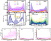 |
Fig. 5. Top panels: Dense Basis SFHs based on the LRD1 (left) and LRD2 (right) PSF photometry. Solid lines show the 50th percentile and shaded regions the 16th-84th percentiles, color-coded by redshift. The thicker line depicts the low-z case, which corresponds to the photo-z of the galaxy group. Middle panels: Dense Basis SFHs derived from the stellar component only (obtained by subtracting the AGN photometry from the PSF photometry; Sect. 4.3), color-coded by redshift. The inset in the left panel shows a zoomed-in view of the LRD1 mid-z SFH. Bottom panels (from left to right): SFHs derived for SAT0, SAT1, and SAT2, color-coded by redshift. |
This quenching is compatible with the prevailing idea that Balmer breaks are associated with evolved stellar populations, although these breaks could also originate from dense gas absorption near the AGN (Inayoshi & Maiolino 2025; see also de Graaff et al. 2025; Ji et al. 2025; Naidu et al. 2025, and Rusakov et al. 2025).
The SFHs obtained based on the stellar component of the stars + AGN scenario (see Sect. 4.3 and the bottom panels in the first row in Fig. 5) yield the same results in the case of LRD2, although with a higher average SFR. For LRD1, the high-z case (a dust-free AGN) provides a burstier, less smooth SFH compared to our previous results. It also reflects a recent burst of star formation, reaching 900 M⊙/yr. According to the mid-z solution, which resembles the obscured AGN, LRD1 formed stars at a very low rate and is currently undergoing a burst of star formation. The mid-z AGN is not a good solution for LRD1 (see Sect. 4.2) and it is only included to illustrate a possible option to describe the LRDs’ SEDs. Further discussion for LRD1 will be based on the SFH provided by the high-z case, keeping in mind that the photo-z of the galaxy group, based on the potential satellites, is slightly lower, but our codes cannot find a good solution if we do not allow a z ∼ 7 fit. Alternative scenarios could also reproduce our observables as well (see Sect. 4.2).
The SFHs of the satellites are displayed in the second row in Fig. 5. SAT0 shows two potential evolutionary pathways, corresponding to the star-forming and the Balmer break solutions. The SFHs of SAT1 and SAT2 are consistent with recent bursts of star formation that started ∼ 100 Myr ago, coincident with the bursts observed in the LRDs.
5. Discussion
The caveats involved in our strategy to investigate the nature of this LRD pair are numerous and difficult to tackle with our data. Spectroscopic redshifts, better sampling of these potential Balmer breaks, and other AGN diagnostics are required. Thus, rather than trying to comprehensively “solve” this system, in this work we aim to establish the basis for future research, providing some hypotheses about the physical processes taking place inside and outside these rich high-z laboratories.
The main novelty of this study is the observation of a pair of LRDs in close proximity (see also Tanaka et al. 2024), embedded in a potential system of satellites at an early stage of the Universe’s life. If these LRDs were Balmer break galaxies, as reported by Dense Basis and Bagpipes, this pair would have gone through recent bursts of star formation, followed by quenching, during the last 200 Myr. The satellites are experiencing bursts of star formation that started 100 Myr ago. This synchronicity is likely not a coincidence and may indicate an interconnection between all these objects. The LRD activity seems to be partially responsible for these bursts in the satellites. Assuming that (i) the LRD1 F410M photometry (considering the brightest source of the LRD pair) is contaminated by Hβ + [OIII]λλ4959, 5007 emission in ≳25% (see Appendix D), and (ii) that ∼10% of this composite emission is due to Hβ at this z, (iii) the total recombination rate coefficient under Case B, (iv) a hydrogen density of ∼10−4 cm−3, (v) A(V) ∼ 1 mag, (vi) and a Strömgren sphere, we can obtain a rough estimate of the size of the ionizing bubble produced by LRD1 at the time of the observation (Leitherer & Heckman 1995). We obtained a radius for this bubble on the order of hundreds of pkpc (∼500 pkpc assuming typical SFG line widths and ∼1 pMpc if we consider typical AGN line widths), which can thus potentially affect the satellites.
On the other hand, the potential interaction of the LRD pair can also be the trigger for the bursts and later quenching reflected in their SFHs (i.e., environmentally driven bursts, and potential environmental quenching). Given the uncertainties in the SFHs, two possible hypotheses arise for the quenching phase: (a) direct environmental quenching and (b) environmentally triggered internal quenching. These scenarios are depicted in Fig. 6 and potential AGN activity is assumed. The SFHs correspond to those shown in the bottom panels, first row, in Fig. 5, which are based on the Dense Basis fits to the stellar component only. As explained in Sect. 4.4, these SFHs are compatible with the SFHs obtained from the untouched PSF LRD photometry, which are also displayed for completeness.
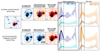 |
Fig. 6. Potential scenarios for the LRDs’ SFHs. Red colors in the image cutouts indicate quenching, orange a quenching in progress, and blue star formation. SAT0 is depicted in black due to its uncertain nature. The two rows show three time steps within the last ∼ 200 Myr, marked in the SFH plots as vertical lines. Case (a) corresponds to direct environmental quenching, and case (b) shows quenching due to internal processes, triggered by the environment. LRD1 is treated as the AGN host, but the same would apply if LRD2 or both LRDs were AGN hosts. In the SFH plots (last two columns), thicker lines highlight the curves used as a reference for each case. We show the SFHs obtained with Dense Basis for the stellar component only (highlighted with thicker borders), derived by subtracting the AGN photometric points from Bagpipes from the PSF photometry (Sect. 4.3). The SFHs based on the untouched PSF photometry (Sect. 4.1) are depicted in the last column. In the panels showing the SFHs based on the stellar component, we represent the LRD1 results for the high-z case in navy (see Sect. 4.2) and the LRD2 results for the low-z case (centered at the photo-z of the galaxy group) in cyan, following the Fig. 5 color code. The low-z SFHs are represented in orange (LRD1) and brown (LRD2) in the last column, which shows the SFHs based on the untouched PSF photometry, following the Fig. 5 color code. The scaling of the SFHs is arbitrary in this cartoon and thus not indicated. |
In case (a), the interaction can lead to the rapid growth of an AGN (in either of the LRDs) by disrupting the corotational motion of the gas in its vicinity (Ricci et al. 2017; Davies et al. 2022). Then, the interplay between dust grains’ sublimation (Alexander et al. 1983) near the AGN and potentially radiation pressure (Ricci et al. 2017; Arakawa et al. 2022) would leave the immediate surroundings of the supermassive black hole (SMBH) relatively dust-free. Although isolated, the SED shapes of LRD CEERS 746 (Kocevski et al. 2023) and CANUCS-LRD-z8.6 (Tripodi et al. 2024) suggest the presence of a broad-line AGN possibly caught in a transition phase between a dust-obscured starburst and an unobscured quasar. This stage would have taken place in one or both of our LRDs ∼ 100 Myr ago. If AGN-driven winds are powerful enough, the galaxy might experience a blow-out where large amounts of gas and dust are stripped from the galaxy, potentially suppressing star formation. These outflows could also quench star formation in the companion LRD. The tidal feature shown in Fig. 1 could actually be probing a potential [OII] and [OIII] outflow emission coming from LRD1.
In case (b), quenching of the AGN host would be delayed with respect to this SMBH rapid growth. If the gas close to the AGN is not highly disturbed (i.e., the merger is less disruptive), then the AGN’s impact is lower (Davies et al. 2022). The host galaxy can benefit from gas inflow and compression due to the interaction, enhanced by the AGN. Quenching in the companion LRD would consequently be caused by mechanisms other than the environment (e.g., stellar feedback, feedback from its own AGN). It is important to acknowledge that, given the environmentally driven nature of the burst, this internal quenching can also be regarded as a consequence of the encounter, with the environment acting as the ultimate triggering phenomenon. The difference in the SFH peaks between the two LRDs in case (b) is, however, ∼50 Myr, which may not be large enough to be regarded as a real difference given the resolution of the SED-fitting code (i.e., we could still be facing case (a)).
In either case (a) or (b), this is one of the first galaxy systems in which we can test a potential relationship between possible AGN triggering, merging, and reddening in LRDs, as well as a merging origin. Our findings suggest that environmental effects might be playing an important role already at z ∼ 7.
It is important to remember that these scenarios are based on the assumption that the Balmer breaks we see are stellar. According to Ji et al. (2025), a combination of an AGN, a Compton-thick dust-free gas cocoon, and different values of the turbulent broadening can produce smooth Balmer breaks that would be more representative of the breaks seen in the LRD population. This scenario would alleviate the problems associated with the high M⋆ and densities of the stellar population that we are seeing. However, the cocoon scenario, while intriguing, is still being explored: the estimated black hole masses are quite high, the formation and evolutionary path of the cocoon are still unclear, not all LRDs show Balmer breaks, and the presence of Balmer absorptions has only been reported in ∼20% of LRDs. This last point could also be due to the lack of high-resolution spectra for these objects, while the absence of these breaks could be related to different evolutionary phases or lower values of the turbulent broadening. Further investigation is required to gain more insight into this possible physical scenario. We note that our LRD pair could naturally fit into this hypothesis, considering that AGN fueling is known to be triggered by host galaxy interactions. We leave the exploration of this possibility to future work.
6. Conclusions
We report the discovery of a LRD pair (dubbed LRD1 and LRD2) at z ∼ 7 (tage ∼ 800 Myr) in the Abell 370 cluster field using JWST/NIRCam data from CANUCS. This pair forms a compact galaxy group together with three potential satellite sources at the same redshift (SAT0, SAT1, and SAT2).
According to our SED analysis, both LRDs could be described with a Balmer break plus a high M⋆ and A(V). The satellites are dust-free and lower-mass sources. There is a UV excess in the LRDs, especially in LRD1, that cannot be attributed to stars according to current models. We show that this excess could be produced by a potential dust-free AGN, although further confirmation is required. The optical continuum would then be powered by obscured star formation plus AGN emission.
The SFHs of the LRD pair show they recently quenched after a burst of star formation that started ∼200 Myr ago, and the satellites have been going through a burst phase that started ∼100 Myr ago. The satellites’ bursts seem to be triggered by their interaction with the LRDs (i.e., interaction-induced bursts; see Asada et al. 2023, 2024). On the other hand, the simultaneous burst and quenching of the LRDs could also have an environmental origin, where a potential AGN would shut down the star formation of the whole pair.
Acknowledgments
This research was enabled by grant 18JWST-GTO1 from the Canadian Space Agency and Discovery Grant and Discovery Accelerator funding from the Natural Sciences and Engineering Research Council (NSERC) of Canada to MS. YA is supported by a Research Fellowship for Young Scientists from the Japan Society for the Promotion of Science (JSPS). MB acknowledges support from the ERC Grant FIRSTLIGHT, Slovenian national research agency ARRS through grants N1-0238 and P1-0188, and the program HST-GO-16667, provided through a grant from the STScI under NASA contract NAS5-26555. This research used the Canadian Advanced Network For Astronomy Research (CANFAR) platform operated in partnership by the Canadian Astronomy Data Centre and The Digital Research Alliance of Canada with support from the National Research Council of Canada, the Canadian Space Agency, CANARIE, and the Canada Foundation for Innovation. This research is in part based on observations made with the NASA/ESA Hubble Space Telescope obtained from the Space Telescope Science Institute, which is operated by the Association of Universities for Research in Astronomy, Inc., under NASA contract NAS 5–26555. HST observations are associated with program HST-GO-15117. This work is based on observations made with the NASA/ESA/CSA James Webb Space Telescope. The data were obtained from the Mikulski Archive for Space Telescopes at the Space Telescope Science Institute, which is operated by the Association of Universities for Research in Astronomy, Inc., under NASA contract NAS 5-03127 for JWST. JWST observations are associated with program JWST-GTO-1208. The data described here may be obtained from https://dx.doi.org/10.17909/xtmj-q319.
References
- Akins, H. B., Casey, C. M., Allen, N., et al. 2023, ApJ, 956, 61 [NASA ADS] [CrossRef] [Google Scholar]
- Akins, H. B., Casey, C. M., Berg, D. A., et al. 2025, ApJ, 980, L29 [Google Scholar]
- Alexander, D. R., Johnson, H. R., & Rypma, R. L. 1983, ApJ, 272, 773 [NASA ADS] [CrossRef] [Google Scholar]
- Ananna, T. T., Bogdán, Á., Kovács, O. E., Natarajan, P., & Hickox, R. C. 2024, ApJ, 969, L18 [NASA ADS] [CrossRef] [Google Scholar]
- Arakawa, N., Fabian, A. C., Ferland, G. J., & Ishibashi, W. 2022, MNRAS, 517, 5069 [NASA ADS] [CrossRef] [Google Scholar]
- Asada, Y., Sawicki, M., Desprez, G., et al. 2023, MNRAS, 523, L40 [NASA ADS] [CrossRef] [Google Scholar]
- Asada, Y., Sawicki, M., Abraham, R., et al. 2024, MNRAS, 527, 11372 [Google Scholar]
- Asada, Y., Desprez, G., Willott, C. J., et al. 2025, ApJ, 983, L2 [Google Scholar]
- Barro, G., Pérez-González, P. G., Kocevski, D. D., et al. 2024, ApJ, 963, 128 [CrossRef] [Google Scholar]
- Bertin, E., & Arnouts, S. 1996, A&AS, 117, 393 [NASA ADS] [CrossRef] [EDP Sciences] [Google Scholar]
- Boylan-Kolchin, M. 2023, Nat. Astron., 7, 731 [NASA ADS] [CrossRef] [Google Scholar]
- Bradley, L. 2023, https://doi.org/10.5281/zenodo.7946442 [Google Scholar]
- Brammer, G. B., van Dokkum, P. G., & Coppi, P. 2008, ApJ, 686, 1503 [Google Scholar]
- Byler, N., Dalcanton, J. J., Conroy, C., & Johnson, B. D. 2017, ApJ, 840, 44 [Google Scholar]
- Calzetti, D., Armus, L., Bohlin, R. C., et al. 2000, ApJ, 533, 682 [NASA ADS] [CrossRef] [Google Scholar]
- Carnall, A. C., McLure, R. J., Dunlop, J. S., & Davé, R. 2018, MNRAS, 480, 4379 [Google Scholar]
- Casey, C. M., Kartaltepe, J. S., Drakos, N. E., et al. 2023, ApJ, 954, 31 [NASA ADS] [CrossRef] [Google Scholar]
- Casey, C. M., Akins, H. B., Kokorev, V., et al. 2024, ApJ, 975, L4 [Google Scholar]
- Chabrier, G. 2003, PASP, 115, 763 [Google Scholar]
- Chen, C.-H., Ho, L. C., Li, R., & Zhuang, M.-Y. 2025, ApJ, 983, 60 [Google Scholar]
- Conroy, C., & Gunn, J. E. 2010, Astrophysics Source Code Library [record ascl:1010.043] [Google Scholar]
- Davies, J. J., Pontzen, A., & Crain, R. A. 2022, MNRAS, 515, 1430 [CrossRef] [Google Scholar]
- de Graaff, A., Rix, H. W., Naidu, R. P., et al. 2025, A&A, submitted [Google Scholar]
- Dekel, A., Sarkar, K. C., Birnboim, Y., Mandelker, N., & Li, Z. 2023, MNRAS, 523, 3201 [NASA ADS] [CrossRef] [Google Scholar]
- Desprez, G., Richard, J., Jauzac, M., et al. 2018, MNRAS, 479, 2630 [Google Scholar]
- Desprez, G., Martis, N. S., Asada, Y., et al. 2024, MNRAS, 530, 2935 [Google Scholar]
- Doyon, R., Willott, C. J., Hutchings, J. B., et al. 2023, PASP, 135, 098001 [NASA ADS] [CrossRef] [Google Scholar]
- Duan, Q., Conselice, C. J., Li, Q., et al. 2025, MNRAS, 540, 774 [Google Scholar]
- Elíasdóttir, Á., Limousin, M., Richard, J., et al. 2007, arXiv e-prints [arXiv:0710.5636] [Google Scholar]
- Ferrara, A. 2024a, A&A, 684, A207 [NASA ADS] [CrossRef] [EDP Sciences] [Google Scholar]
- Ferrara, A. 2024b, A&A, 689, A310 [NASA ADS] [CrossRef] [EDP Sciences] [Google Scholar]
- Ferrara, A., Pallottini, A., & Dayal, P. 2023, MNRAS, 522, 3986 [NASA ADS] [CrossRef] [Google Scholar]
- Gardner, J. P., Mather, J. C., Abbott, R., & Zondag, E. 2023, PASP, 135, 068001 [CrossRef] [Google Scholar]
- Gentile, F., Casey, C. M., Akins, H. B., et al. 2024, ApJ, 973, L2 [NASA ADS] [CrossRef] [Google Scholar]
- Gledhill, R., Strait, V., Desprez, G., et al. 2024, ApJ, 973, 77 [CrossRef] [Google Scholar]
- Greene, J. E., Labbe, I., Goulding, A. D., et al. 2024, ApJ, 964, 39 [CrossRef] [Google Scholar]
- Hainline, K. N., Maiolino, R., Juodžbalis, I., et al. 2025, ApJ, 979, 138 [Google Scholar]
- Hutter, A., Cueto, E. R., Dayal, P., et al. 2025, A&A, 694, A254 [NASA ADS] [CrossRef] [EDP Sciences] [Google Scholar]
- Inayoshi, K., & Maiolino, R. 2025, ApJ, 980, L27 [Google Scholar]
- Inoue, A. K., Shimizu, I., Iwata, I., & Tanaka, M. 2014, MNRAS, 442, 1805 [NASA ADS] [CrossRef] [Google Scholar]
- Iyer, K., & Gawiser, E. 2017, ApJ, 838, 127 [NASA ADS] [CrossRef] [Google Scholar]
- Iyer, K. G., Gawiser, E., Faber, S. M., et al. 2019, ApJ, 879, 116 [NASA ADS] [CrossRef] [Google Scholar]
- Jakobsen, P., Ferruit, P., Alves de Oliveira, C., et al. 2022, A&A, 661, A80 [NASA ADS] [CrossRef] [EDP Sciences] [Google Scholar]
- Ji, X., Maiolino, R., Übler, H., et al. 2025, MNRAS, submitted [arXiv:2501.13082] [Google Scholar]
- Jullo, E., Kneib, J. P., Limousin, M., et al. 2007, New J. Phys., 9, 447 [Google Scholar]
- Killi, M., Watson, D., Brammer, G., et al. 2024, A&A, 691, A52 [NASA ADS] [CrossRef] [EDP Sciences] [Google Scholar]
- Kneib, J. P., Ellis, R. S., Smail, I., Couch, W. J., & Sharples, R. M. 1996, ApJ, 471, 643 [Google Scholar]
- Kocevski, D. D., Onoue, M., Inayoshi, K., et al. 2023, ApJ, 954, L4 [NASA ADS] [CrossRef] [Google Scholar]
- Kocevski, D. D., Finkelstein, S. L., Barro, G., et al. 2024, ApJ, accepted [arXiv:2404.03576] [Google Scholar]
- Kokorev, V., Caputi, K. I., Greene, J. E., et al. 2024, ApJ, 968, 38 [NASA ADS] [CrossRef] [Google Scholar]
- Labbé, I., van Dokkum, P., Nelson, E., et al. 2023, Nature, 616, 266 [CrossRef] [Google Scholar]
- Labbe, I., Greene, J. E., Matthee, J., et al. 2024, ApJ, submitted [arXiv:2412.04557] [Google Scholar]
- Labbe, I., Greene, J. E., Bezanson, R., et al. 2025, ApJ, 978, 92 [NASA ADS] [CrossRef] [Google Scholar]
- Larson, R. L., Hutchison, T. A., Bagley, M., et al. 2023, ApJ, 958, 141 [NASA ADS] [CrossRef] [Google Scholar]
- Leitherer, C., & Heckman, T. M. 1995, ApJS, 96, 9 [NASA ADS] [CrossRef] [Google Scholar]
- Leja, J., Carnall, A. C., Johnson, B. D., Conroy, C., & Speagle, J. S. 2019, ApJ, 876, 3 [Google Scholar]
- Li, Z., Dekel, A., Sarkar, K. C., et al. 2024, A&A, 690, A108 [NASA ADS] [CrossRef] [EDP Sciences] [Google Scholar]
- Li, Z., Inayoshi, K., Chen, K., Ichikawa, K., & Ho, L. C. 2025, ApJ, 980, 36 [Google Scholar]
- Limousin, M., Kneib, J.-P., & Natarajan, P. 2005, MNRAS, 356, 309 [Google Scholar]
- Ma, Y., Greene, J. E., Setton, D. J., et al. 2025, ApJ, 981, 191 [Google Scholar]
- Maiolino, R., Risaliti, G., Signorini, M., et al. 2025, MNRAS, 538, 1921 [Google Scholar]
- Markov, V., Gallerani, S., Pallottini, A., et al. 2023, A&A, 679, A12 [NASA ADS] [CrossRef] [EDP Sciences] [Google Scholar]
- Markov, V., Gallerani, S., Ferrara, A., et al. 2025, Nat. Astron., 9, 458 [Google Scholar]
- Martis, N. S., Sarrouh, G. T. E., Willott, C. J., et al. 2024, ApJ, 975, 76 [NASA ADS] [CrossRef] [Google Scholar]
- Matthee, J., Naidu, R. P., Brammer, G., et al. 2024, ApJ, 963, 129 [NASA ADS] [CrossRef] [Google Scholar]
- Menci, N., Castellano, M., Santini, P., et al. 2022, ApJ, 938, L5 [NASA ADS] [CrossRef] [Google Scholar]
- Mirocha, J., & Furlanetto, S. R. 2023, MNRAS, 519, 843 [Google Scholar]
- Naidu, R. P., Matthee, J., Katz, H., et al. 2025, arXiv e-prints [arXiv:2503.16596] [Google Scholar]
- Narayanan, D., Lower, S., Torrey, P., et al. 2024, ApJ, 961, 73 [NASA ADS] [CrossRef] [Google Scholar]
- Nenkova, M., Sirocky, M. M., Nikutta, R., Ivezić, Ž., & Elitzur, M. 2008, ApJ, 685, 160 [Google Scholar]
- Noirot, G., Desprez, G., Asada, Y., et al. 2023, MNRAS, 525, 1867 [NASA ADS] [CrossRef] [Google Scholar]
- Oke, J. B., & Gunn, J. E. 1983, ApJ, 266, 713 [NASA ADS] [CrossRef] [Google Scholar]
- Pallottini, A., & Ferrara, A. 2023, A&A, 677, L4 [NASA ADS] [CrossRef] [EDP Sciences] [Google Scholar]
- Pérez-González, P. G., Barro, G., Annunziatella, M., et al. 2023, ApJ, 946, L16 [CrossRef] [Google Scholar]
- Pérez-González, P. G., Barro, G., Rieke, G. H., et al. 2024, ApJ, 968, 4 [CrossRef] [Google Scholar]
- Perger, K., Fogasy, J., Frey, S., & Gabányi, K. É. 2025, A&A, 693, L2 [NASA ADS] [CrossRef] [EDP Sciences] [Google Scholar]
- Ricci, C., Bauer, F. E., Treister, E., et al. 2017, MNRAS, 468, 1273 [NASA ADS] [Google Scholar]
- Rieke, M. J., Kelly, D. M., Misselt, K., et al. 2023, PASP, 135, 028001 [CrossRef] [Google Scholar]
- Rusakov, V., Watson, D., Nikopoulos, G. P., et al. 2025, Nature, submitted [arXiv:2503.16595] [Google Scholar]
- Sarrouh, G. T. E., Muzzin, A., Iyer, K. G., et al. 2024, ApJ, 967, L17 [Google Scholar]
- Setton, D. J., Greene, J. E., de Graaff, A., et al. 2024, ApJ, submitted [arXiv:2411.03424] [Google Scholar]
- Simha, V., Weinberg, D. H., Conroy, C., et al. 2014, MNRAS, submitted [arXiv:1404.0402] [Google Scholar]
- Steinhardt, C. L., Jauzac, M., Acebron, A., et al. 2020, ApJS, 247, 64 [Google Scholar]
- Tanaka, T. S., Silverman, J. D., Shimasaku, K., et al. 2024, PASJ, submitted [arXiv:2412.14246] [Google Scholar]
- Temple, M. J., Hewett, P. C., & Banerji, M. 2021, MNRAS, 508, 737 [NASA ADS] [CrossRef] [Google Scholar]
- Trinca, A., Schneider, R., Valiante, R., et al. 2024, MNRAS, 529, 3563 [NASA ADS] [CrossRef] [Google Scholar]
- Tripodi, R., Martis, N., Markov, V., et al. 2024, Nat. Commun., submitted [arXiv:2412.04983] [Google Scholar]
- Vanden Berk, D. E., Richards, G. T., Bauer, A., et al. 2001, AJ, 122, 549 [Google Scholar]
- Vilella-Rojo, G., Viironen, K., López-Sanjuan, C., et al. 2015, A&A, 580, A47 [NASA ADS] [CrossRef] [EDP Sciences] [Google Scholar]
- Wang, B., Leja, J., de Graaff, A., et al. 2024, ApJ, 969, L13 [NASA ADS] [CrossRef] [Google Scholar]
- Whitler, L., Stark, D. P., Endsley, R., et al. 2023, MNRAS, 519, 5859 [NASA ADS] [CrossRef] [Google Scholar]
- Williams, C. C., Alberts, S., Ji, Z., et al. 2024, ApJ, 968, 34 [NASA ADS] [CrossRef] [Google Scholar]
- Willott, C. J., Doyon, R., Albert, L., et al. 2022, PASP, 134, 025002 [CrossRef] [Google Scholar]
- Yuma, S., Ohta, K., Yabe, K., et al. 2010, ApJ, 720, 1016 [Google Scholar]
- Zhang, Z., Jiang, L., Liu, W., & Ho, L. C. 2025, ApJ, 985, 119 [Google Scholar]
- Ziparo, F., Ferrara, A., Sommovigo, L., & Kohandel, M. 2023, MNRAS, 520, 2445 [NASA ADS] [CrossRef] [Google Scholar]
Appendix A: Lens model
Gledhill et al. (2024) reported an improved gravitational lensing model for Abell 370 using NIRCam and NIRISS data from CANUCS. Additionally, we developed a local lens model for this sample, given that our sources are located over 3 from the cluster center, far from the strong lensing constraints, and close to three bright foreground sources, which were not considered in the Gledhill et al. (2024) strong lensing model. Upon visual inspection, we found that one of the three foreground galaxies (at ∼8″ from the LRD pair) features a galaxy-galaxy lensing system and is surrounded by four multiple images of a background source (see Fig. A.1). Despite the light contamination from the foreground galaxy, we could identify the background source as an F090W dropout z ∼ 7 source. We include the positions of the identified multiple images of this source in Table A.2. As shown in Desprez et al. (2018), galaxy-galaxy lensing systems on the outskirts of clusters serve as powerful probes of the local lensing properties at large distances where no other strong lensing constraints are available. We therefore used the newly discovered galaxy-galaxy lensing system to constrain our local lens model and accounted for the external shear from the cluster potential. We also note its potential utility for future strong lensing analysis of Abell 370.
This local lens model was constrained with Lenstool (Kneib et al. 1996, Jullo et al. 2007) and consists of three halos following a dual Pseudo Isothermal Elliptical density profile (Limousin et al. 2005, Elíasdóttir et al. 2007). The elliptical galaxy lensing the background source was modeled with a free central velocity dispersion. The other two galaxies were added as fixed potentials: we modeled the spiral galaxy at 5″ away from the LRD pair and the elliptical galaxy at 12″ (see Fig. A.1), with cluster member scaling relations constrained by Gledhill et al. (2024) in the inner cluster regions, using F090W = 20.14 and 20.89 mag, respectively. The ellipticities and orientations of the three galaxies were fixed, following the light distribution. The cut and core radii of all three galaxies were also obtained from the Gledhill et al. (2024) scaling relations. Following the single lens plane approach, which is conventionally used in cluster lensing analysis (e.g., Gledhill et al. 2024), we modeled the sources (with EAzY redshifts between 0.16 and 0.56) at cluster redshift. Apart from the three galaxy halos, we added the external shear with free strength and orientation to account for the contribution of the galaxy cluster.
Positions of our galaxies corrected for lensing relative to α= 40.009161, δ = −1.620810 (deg).
IDs and coordinates of the background source’s multiple images, lensed by a foreground galaxy near the LRD pair.
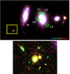 |
Fig. A.1. Top: 19×11 arcsec2 cutout of an RGB image based on F277W, F410M, and F444W centered around coordinates α= 2:40:02.338, δ = −1:37:15.297. The yellow square encloses the region that contains our galaxies; its dimensions are 2.8 × 2.4 arcsec2. The four multiple images of the z ∼ 7 background source are highlighted with green circles and labeled with the IDs listed in Table A.2. The green colors highlight this source’s F410M excess; we also noticed F410M excess in our galaxy sample, suggesting they are at similar redshifts. Bottom: 4×3 arcsec2 cutout of the same RGB image around our sample, with the scale saturated to also show SAT1 and SAT2. The source-plane positions of the sources after the lensing correction are depicted as crosses (yellow for the LRDs and green for the satellites). |
Appendix B: Photometry measurements
Photometry of this galaxy group.
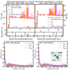 |
Fig. B.1. Dense Basis stellar fits and SFHs derived for SAT1b and SAT1. We include a F150W cutout of SAT1 that shows its different components in the bottom right panel. See Fig. 2 for a description of the color codes. |
PSF photometry was measured using photutils in PSF-convolved images homogenized to the F444W resolution (Sarrouh et al. 2024). We used the empirical PSFs, obtained by median-stacking non-saturated bright stars (Sarrouh et al. 2024). The aperture radius, used to estimate the initial flux of each source, was set to 3 pixels, with fit_shape = (3, 3). Both the fluxes and uncertainties (derived from the residuals of the PSF fit) correspond to the values reported by psfphot. Photometric points were then corrected for Galactic extinction. In Table B.1 we show the photometry measured for each of these galaxies.
SAT1, whose analysis in this work is based on aperture photometry, shows signs of a multi-component structure. The main goal of this paper is to try to understand the nature of the LRD pair and determine whether there is evidence of a connection between all the galaxies in this potential group via their SFHs. Understanding the full complexity of SAT1 is beyond the scope of this work. Nevertheless, we offer a possible segmentation for this object, as well as the PSF photometry, Dense Basis SED fitting, and SFHs of its main component, SAT1b, in Fig. B.1. The emission of SAT1 seems to be dominated by SAT1b, located at z ∼ 6.79. It is a ∼108 M⊙ source with A(V) ∼0.1 mag according to Dense Basis. SAT1a could be a lower-z source (z ∼ 5.9) while SAT1c, which seems to be a clump or satellite of SAT1b, is located at z ∼ 6.77.
Appendix C: SAT3
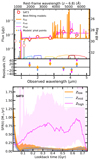 |
Fig. C.1. Dense Basis stellar fits and SFHs for SAT3. See Fig. 2 for a description of the color codes. |
The first row in Fig. C.1 shows the 0.3″ aperture photometry from the CANUCS catalog of source #2104938, dubbed SAT3 in Sect. 3.1, together with the Dense Basis stellar fits. This galaxy is located at z ∼ 6.79, corresponds to a 108 M⊙ source, and is subject to a low dust attenuation (A(V) ∼0.2 mag), showing similar properties to SAT1 and SAT2. The low- and mid-z SED fits point to an SFG, while the high-z solution fits a Balmer break, as also seen in SAT0. As in that case, the colors of this source favor the SFG scenario. The SFHs associated with each of the z intervals are displayed in the second row in Fig. C.1. The low- and mid-z cases depict a recent burst of star formation, similar to those seen in the SFHs of SAT1 and SAT2.
Appendix D: The Dense Basis method
As specified in Sect. 4.1, for the Dense Basis fits the M⋆ was constrained between 7 < log M⋆/M⊙ < 12 and the SFR between −1 < log SFR[M⊙/yr]< 3, setting a flat specific SFR. For parameters such as dust attenuations or metallicities, the default Dense Basis configuration was used, which considers a Calzetti et al. (2000) dust attenuation law. This assumption for the attenuation is reasonable for our galaxies, as the dust curves at z > 6 are commonly found to be flat and lack a prominent UV bump (Markov et al. 2023, 2025). In Tripodi et al. (2024) we adopted a flexible analytical attenuation model for an LRD at z ∼ 8. The resulting attenuation curve was Calzetti-like, though slightly shallower in the rest-frame UV. However, changes in the shape of the curve had a considerable impact on the inferred A(V) by ∼0.6 dex. This, in turn, affects other fundamental galaxy properties to a lesser extent, such as M⋆, SFR, or stellar age by 0.2 − 0.4 dex. We cannot provide better constraints on the attenuation with our current data and insist on keeping this possible degeneracy in mind.
We selected what we called a low- (6.75 < z < 6.85, centered at the photo-z of the galaxy group), mid- (6.75 < z < 6.95), and high-z (6.95 < z < 7.15) intervals for the redshift priors.
Dense Basis identifies a best-fitting solution for each source looking for the model within the atlas (which is set according to the selected priors) that maximizes the likelihood. Upper and lower bounds for each parameter are then computed based on the 100 best models for each galaxy. This approach will penalize those templates that exhibit a slight deviation from the points with the highest S/N (in our case the red points: the F356W, F410M, and F444W data). Conversely, it will be more flexible in selecting how the lower S/N points are fitted (the blue points: the F150W, F200M, and F277W data). This is not an issue for the satellites, which are typical SFGs and are easily reproduced by current models. However, LRDs are still not well represented by any known template.
Figures D.1 (based on the LRD PSF photometry) and D.2 (based on the stellar component only) depict the best-fitting models obtained directly with this code for the LRD pair. In some of the cases, Dense Basis yielded best-fitting models that could reproduce the red slopes by selecting a Balmer break, but these models exhibited a UV slope that was either steeper or flatter than the observed one. An illustrative example of such models is provided in the right panel of Fig. D.1 (orange curve) and in the right panel of Fig. D.2 (yellow curve).
An alternative option would be to fit the LRDs with two different model components and two different slopes (see Killi et al. 2024, Setton et al. 2024). However, this approach does not align with the scientific goal of this work, as these fits would not allow us to establish a connection between the photometry and the SFHs.
In an attempt to obtain a model that balances the fitting of both the red and blue points, we opted to iteratively increase the uncertainties of the red data in some percentage of the flux. This provides more freedom to Dense Basis, which can slightly deviate from the trend defined by the red points while looking for a more suitable solution for the UV. The uncertainties of the red points were increased in 0 − 2% of the flux in 0.05% steps while keeping the best-fitting model for each iteration. To select the final most probable solution, we compared the models’ slopes defined by the continuum around different parts of the SED with those directly measured from the data. We defined a red slope by means of a linear fit to the F356W and F444W data points; a blue slope, using the F150W, F200W, and F277W filters; and the break, based on the F277W and F356W emission. We kept the 10 best-fitting models that minimized the ratio between the observed and the model’s red slopes and then selected the model that minimized the ratios of the blue slopes and the breaks.
We are aware that this approach will preferentially select Balmer break solutions in which the red points probe the continuum redward of the break instead of models of highly SFGs where these are partially or totally boosted by strong emission lines. Nevertheless, this approach was also used to fit the SEDs of the satellites, resulting in the recovery of star-forming solutions with no breaks. On the other hand, as already mentioned, Dense Basis also favors the presence of a Balmer Break without additional constraints on the code. Furthermore, we also explored selecting a more restrictive prior on the attenuation and SFR to force a highly star-forming solution. We set A(V) > 0.8 mag and 1< log SFR[M⊙/yr]< 3 for the priors. However, during the fitting process, Dense Basis rescaled these values and continued selecting Balmer break solutions with lower SFRs.
If we therefore assume that these LRDs have a Balmer break, part of the emission could still be powered by lines contaminating the broadband photometry. This would have a direct impact on our stellar mass estimates, which could be larger than the actual M⋆ (see Desprez et al. 2024). At the redshifts considered in this work, the F356W, F410M, and F444W points may be contaminated by the Hβ+[OIII]λλ4959, 5007 composite emission, whereas the [OII]λλ3726, 3729 doublet may boost the F277W filter. Only if z ≳ 7.0 we can assume that the F356W filter is free from emission lines, thereby allowing us to probe the continuum. In that case, the three-filter method described in Vilella-Rojo et al. (2015) can be used to measure the contamination of these lines in the F410M and F444W filters, and define the continuum redward of the break. According to this method, the Hβ+[OIII]λλ4959, 5007 emission would be responsible for ∼11% of the flux in F444W and ∼25% of the flux in F410M in the case of LRD1 (∼11% and ∼24% in the case of LRD2). Running Dense Basis using the line-corrected fluxes yields similar M⋆ compared to the results based on the original photometry, with ∼0.26 dex and ∼0.10 dex lower M⋆ values for LRD1 and LRD2, respectively. However, this correction is quite uncertain, given that we are assuming that the F356W filter is free from e-line emission and that we are also not correcting the F277W filter for possible contamination. Additionally, outshining of older stars by young low-metallicity stars becomes important at z > 7, which can also lead to bad estimations of the M⋆ (Narayanan et al. 2024, Whitler et al. 2023). These are all reminders that our results for the M⋆ of the LRD pair should only be considered with extreme caution.
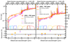 |
Fig. D.1. Stellar fits obtained directly with Dense Basis based on the LRD1 (left) and LRD2 (right) PSF photometry. See Fig. 2 for a description of the markers and color codes. |
Model parameters, priors, and 50th percentile posterior values for LRD1 and LRD2.
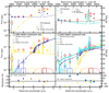 |
Fig. D.2. Stellar fits obtained directly with Dense Basis based on the stellar component (derived by subtracting the Bagpipes AGN photometry from the PSF photometry) of LRD1 (left) and LRD2 (right) PSF photometry (see Sect. 4.3). See Fig. 4 for a description of the markers and color codes. |
Appendix E: The Bagpipes method
Bagpipes is a Python software that utilizes a Bayesian inference approach to estimate physical parameters of galaxies using spectroscopic and/or photometric data. We fitted the photometric points of the two LRDs using a composite model consisting of a stellar population plus an AGN. Initial tests employing only single AGN components or solely stellar populations did not yield satisfactory results. Specifically, when fitting only the stellar component, Bagpipes encountered similar issues as Dense Basis, identifying a Balmer break galaxy that fails to reproduce the blue part of the spectrum and the flux in the F277W filter. Similarly, a model with only an AGN component failed to account for the blue part of the spectrum due to the limitations of the rising power-law continuum. All fits were performed using the Multinest sampling algorithm.
The composite model comprises several parameters:
-
The AGN continuum emission was modeled as a broken power law characterized by three parameters: two spectral slopes and the continuum flux at the break point (5100 Å).
-
The AGN emission line included as a single Hβ emission line, modeled with two free parameters: line width and line intensity.
-
The SFH was modeled using a double power law, enabling the representation of both quenched galaxies and SFGs while minimizing the number of free parameters. The free parameters include the two slopes, the decay timescale (τ), the stellar mass formed, metallicity, and the time when the stars started to form (age).
-
Nebular emission was incorporated via the ionization parameter U.
-
We modeled the dust extinction with the visual extinction parameter A(V), following the Calzetti attenuation law. A dust emission component was not included, as significant emission from hot dust is only expected for λ < 1 μm.
Note that the emission due to the [OIII]λλ4959, 5007 lines is included through the ionization parameter U (Byler et al. 2017). In fact, these lines are present in the mid-z solution shown in Fig. E.1. However, this emission is indistinguishable from the Hβ line in our photometric data, i.e., Bagpipes cannot accurately assign the corresponding separate fluxes to [OIII] and Hβ. We would need a better sampling of the SED to carry out a more detailed and complex modeling of these galaxies.
The redshift parameter was treated in two ways. First, we applied the same prior intervals used in the Dense Basis fits (high, mid, and low-z priors, as shown in Table E.1). Second, we employed a broader uniform prior ranging 6.7 < z < 7.1, encompassing all the other intervals. For LRD1, the broader prior produced a Gaussian posterior distribution consistent with the high-z prior, where the 50th percentile aligns with the posterior peak (see Fig. 3). In contrast, the mid-z prior (Fig. E.1) resulted in a non-Gaussian posterior peaking beyond the upper limit, causing a discrepancy between the 50th percentile and the peak. For the mid-z prior, the AGN parameters’ posterior distributions also lose their Gaussian shape. For the low-z prior, Bagpipes failed to converge to a solution with the same parameter set.
For LRD2, the redshift behavior was similar. The high-z prior yielded a Gaussian posterior (Fig. 3), while the mid and low-z priors still peaked around z ∼ 7 (Fig. E.2). However, Bagpipes successfully converged for the low-z interval in this case.
All model parameters, along with their prior distributions and posterior 50th percentile values, are summarized in Table E.1 for both LRDs. The prior distributions and limits follow those used by Tripodi et al. (2024).
Appendix F: Physical properties
We report the physical parameters derived with Dense Basis and Bagpipes for our galaxy system in Table F.1.
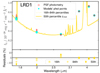 |
Fig. F.1. Bagpipes fit (stars+AGN) for LRD1 based on PSF photometry (red open circles), corresponding to the mid-z case. The best-fitting model is shown as a thick yellow line (50th percentile). See Fig. 3 for a full description of the color codes and markers. |
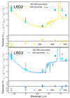 |
Fig. F.2. Bagpipes fit (stars+AGN) for LRD2 based on PSF photometry (red open circles), corresponding to the mid-z (top) and low-z (bottom) cases. Best-fitting models are shown as yellow (top) and blue (bottom) thick lines (50th percentile). See Fig. 3 for a full description of the color codes and markers. |
Physical properties of the galaxy group.
All Tables
Values for the criteria established in Kokorev et al. (2024) and Kocevski et al. (2024), defined in Sect. 3.2, obtained for the LRD pair and SAT0.
Positions of our galaxies corrected for lensing relative to α= 40.009161, δ = −1.620810 (deg).
IDs and coordinates of the background source’s multiple images, lensed by a foreground galaxy near the LRD pair.
Model parameters, priors, and 50th percentile posterior values for LRD1 and LRD2.
All Figures
|
Fig. 1. Cutouts of the galaxy group in different bands. (1): 8 × 8 arcsec2 cutouts of two RGB images based on F277W, F410M, and F444W (left) and F150W, F200W, and F444W (right) NIRCam imaging. The yellow square encloses the region that contains our galaxies; its dimensions are 2.8 × 2.4 arcsec2. These images highlight the common F410M excess (and thus the high-z nature) in this galaxy group compared to sources in the neighborhood (left) and the more prominent emission in F444W of the LRD pair compared to the satellites (right). The red squares in both panels show a zoomed-in view of the LRD pair in a less saturated scale to highlight the difference in color between the LRDs and SAT0. The arrow in the left panel points to a z ∼ 7 source ∼18 kpc away from the LRD pair, with colors similar to the satellite galaxies. (2): Cutouts of our galaxy group in smoothed versions of F200W, F277W, and F410M obtained using a Gaussian filter with σ = 1.2 pixels. (3): Postage stamps of these sources in the different HST and NIRCam bands at native spatial resolution. NIRCam images are plotted following the same scale as above. For the HST bands, the upper limit was set to 3 nJy to deal with the noise. The kiloparsec scale is not corrected for lensing magnification, which is also low at this position and redshift (μ = 1.26; see Fig. A.1). |
| In the text | |
|
Fig. 2. (a): Dense Basis stellar fits based on the LRD1 (left) and LRD2 (right) PSF photometry (red open circles). Data points excluded from the fits are shown using thinner lines. Solid orange, blue, and fuchsia lines depict the fits for the low- (thicker line, corresponding to the photo-z of the galaxy group), mid-, and high-z intervals. The corresponding model photometric points are shown with filled circles. (b): Dense Basis stellar fits for the satellite galaxies based on PSF (SAT0) and aperture (SAT1, SAT2) photometry, following the same color code as above. We include the HST and NIRCam transmission curves, as well as the residuals of the fits. |
| In the text | |
|
Fig. 3. Bagpipes best fits (stars + AGN) for LRD1 (left) and LRD2 (right) based on PSF photometry (red open circles), corresponding to the high-z solution obtained using a broad z prior. Cyan circles depict the synthetic photometric points associated with the best-fitting model, shown as a thick blue line (50th percentile). The limits of the shaded blue region represent the 16th and 84th percentiles. The residuals for the models, corresponding to the 16th (squares), 50th (diamonds), and 84th (circles) percentiles, are also included underneath each panel. |
| In the text | |
|
Fig. 4. Top panels: Potential AGN fits (dashed cyan for the low-z, yellow for the mid-z, navy for the high-z cases) for LRD1 (left) and LRD2 (right) derived using Bagpipes (Sect. 4.2). The low-z case is not represented in the LRD1 panel (left) because it did not converge in Bagpipes. Crosses depict their photometric points. Middle panels: Dense Basis fits for the stellar component of LRD1 (left) and LRD2 (right) obtained by subtracting the AGN photometry derived with Bagpipes from the PSF photometry (Sect. 4.3). The LRD PSF photometry is shown as red open circles. Photometric points from the stellar component are shown as cyan, yellow, and navy open circles for the low-, mid-, and high-z cases, respectively. Best-fit models are displayed as solid lines in the same color. The low-z case (thicker line) corresponds to the photo-z of the galaxy group. Photometric points for the models are depicted as filled circles. HST and NIRCam transmission curves are also included. Bottom panels: Residuals of the fits. |
| In the text | |
|
Fig. 5. Top panels: Dense Basis SFHs based on the LRD1 (left) and LRD2 (right) PSF photometry. Solid lines show the 50th percentile and shaded regions the 16th-84th percentiles, color-coded by redshift. The thicker line depicts the low-z case, which corresponds to the photo-z of the galaxy group. Middle panels: Dense Basis SFHs derived from the stellar component only (obtained by subtracting the AGN photometry from the PSF photometry; Sect. 4.3), color-coded by redshift. The inset in the left panel shows a zoomed-in view of the LRD1 mid-z SFH. Bottom panels (from left to right): SFHs derived for SAT0, SAT1, and SAT2, color-coded by redshift. |
| In the text | |
|
Fig. 6. Potential scenarios for the LRDs’ SFHs. Red colors in the image cutouts indicate quenching, orange a quenching in progress, and blue star formation. SAT0 is depicted in black due to its uncertain nature. The two rows show three time steps within the last ∼ 200 Myr, marked in the SFH plots as vertical lines. Case (a) corresponds to direct environmental quenching, and case (b) shows quenching due to internal processes, triggered by the environment. LRD1 is treated as the AGN host, but the same would apply if LRD2 or both LRDs were AGN hosts. In the SFH plots (last two columns), thicker lines highlight the curves used as a reference for each case. We show the SFHs obtained with Dense Basis for the stellar component only (highlighted with thicker borders), derived by subtracting the AGN photometric points from Bagpipes from the PSF photometry (Sect. 4.3). The SFHs based on the untouched PSF photometry (Sect. 4.1) are depicted in the last column. In the panels showing the SFHs based on the stellar component, we represent the LRD1 results for the high-z case in navy (see Sect. 4.2) and the LRD2 results for the low-z case (centered at the photo-z of the galaxy group) in cyan, following the Fig. 5 color code. The low-z SFHs are represented in orange (LRD1) and brown (LRD2) in the last column, which shows the SFHs based on the untouched PSF photometry, following the Fig. 5 color code. The scaling of the SFHs is arbitrary in this cartoon and thus not indicated. |
| In the text | |
|
Fig. A.1. Top: 19×11 arcsec2 cutout of an RGB image based on F277W, F410M, and F444W centered around coordinates α= 2:40:02.338, δ = −1:37:15.297. The yellow square encloses the region that contains our galaxies; its dimensions are 2.8 × 2.4 arcsec2. The four multiple images of the z ∼ 7 background source are highlighted with green circles and labeled with the IDs listed in Table A.2. The green colors highlight this source’s F410M excess; we also noticed F410M excess in our galaxy sample, suggesting they are at similar redshifts. Bottom: 4×3 arcsec2 cutout of the same RGB image around our sample, with the scale saturated to also show SAT1 and SAT2. The source-plane positions of the sources after the lensing correction are depicted as crosses (yellow for the LRDs and green for the satellites). |
| In the text | |
|
Fig. B.1. Dense Basis stellar fits and SFHs derived for SAT1b and SAT1. We include a F150W cutout of SAT1 that shows its different components in the bottom right panel. See Fig. 2 for a description of the color codes. |
| In the text | |
|
Fig. C.1. Dense Basis stellar fits and SFHs for SAT3. See Fig. 2 for a description of the color codes. |
| In the text | |
|
Fig. D.1. Stellar fits obtained directly with Dense Basis based on the LRD1 (left) and LRD2 (right) PSF photometry. See Fig. 2 for a description of the markers and color codes. |
| In the text | |
|
Fig. D.2. Stellar fits obtained directly with Dense Basis based on the stellar component (derived by subtracting the Bagpipes AGN photometry from the PSF photometry) of LRD1 (left) and LRD2 (right) PSF photometry (see Sect. 4.3). See Fig. 4 for a description of the markers and color codes. |
| In the text | |
|
Fig. F.1. Bagpipes fit (stars+AGN) for LRD1 based on PSF photometry (red open circles), corresponding to the mid-z case. The best-fitting model is shown as a thick yellow line (50th percentile). See Fig. 3 for a full description of the color codes and markers. |
| In the text | |
|
Fig. F.2. Bagpipes fit (stars+AGN) for LRD2 based on PSF photometry (red open circles), corresponding to the mid-z (top) and low-z (bottom) cases. Best-fitting models are shown as yellow (top) and blue (bottom) thick lines (50th percentile). See Fig. 3 for a full description of the color codes and markers. |
| In the text | |
Current usage metrics show cumulative count of Article Views (full-text article views including HTML views, PDF and ePub downloads, according to the available data) and Abstracts Views on Vision4Press platform.
Data correspond to usage on the plateform after 2015. The current usage metrics is available 48-96 hours after online publication and is updated daily on week days.
Initial download of the metrics may take a while.