| Issue |
A&A
Volume 691, November 2024
|
|
|---|---|---|
| Article Number | A52 | |
| Number of page(s) | 12 | |
| Section | Extragalactic astronomy | |
| DOI | https://doi.org/10.1051/0004-6361/202348857 | |
| Published online | 28 October 2024 | |
Deciphering the JWST spectrum of a ‘little red dot’ at z ∼ 4.53: An obscured AGN and its star-forming host
1
Cosmic Dawn Center (DAWN), Jagtvej 128, 2200 Copenhagen N, Denmark
2
Niels Bohr Institute, University of Copenhagen, Lyngbyvej 2, 2100 Copenhagen Ø, Denmark
3
Instituto de Estudios Astrofícos, Facultad de Ingeniería y Ciencias, Universidad Diego Portales, Av. Ejército 441, Santiago 8370191, Chile
4
David A. Dunlap Department of Astronomy & Astrophysics, University of Toronto, 50 St George Street, Toronto, ON M5S 3H4, Canada
5
Department of Physics, Clark University, Worcester, MA 01610-1477, USA
6
Space Telescope Science Institute (STScI), 3700 San Martin Drive, Baltimore, MD 21218, USA
7
Association of Universities for Research in Astronomy (AURA) for the European Space Agency (ESA), STScI, Baltimore, MD, USA
8
Center for Astrophysical Sciences, Department of Physics and Astronomy, The Johns Hopkins University, 3400 N Charles St., Baltimore, MD 21218, USA
⋆ Corresponding author; meghana.killi@mail.udp.cl
Received:
5
December
2023
Accepted:
18
September
2024
JWST has revealed a class of numerous, extremely compact sources with rest-frame red optical/near-infrared (NIR) and blue ultraviolet (UV) colours nicknamed ‘little red dots’. We present one of the highest signal-to-noise ratio JWST NIRSpec prism spectra of a little red dot, J0647_1045 at z = 4.5319 ± 0.0001, and examine its NIRCam morphology to differentiate the origin of the UV and optical/NIR emission and elucidate the nature of the little red dot phenomenon. J0647_1045 is unresolved (re ≲ 0.17 kpc) in the three NIRCam long-wavelength filters but significantly extended (re = 0.45 ± 0.06 kpc) in the three short-wavelength filters, indicating a red compact source in a blue star-forming galaxy. The spectral continuum shows a clear change in slope, from blue in the optical/UV to red in the rest-frame optical/NIR, which is consistent with two distinct components fit by power laws with different attenuations: AV = 0.38 ± 0.01 (UV) and AV = 5.61 ± 0.04 (optical/NIR). Fitting the Hα line requires both broad (full width at half maximum of ∼4300 ± 100 km s−1) and narrow components, but none of the other emission lines, including Hβ, show evidence of broadness. We calculated AV = 0.9 ± 0.4 from the Balmer decrement using narrow Hα and Hβ and AV > 4.1 ± 0.1 from broad Hα and an upper limit on broad Hβ, which is consistent with blue and red continuum attenuation, respectively. Based on a single-epoch Hα line width, the mass of the central black hole is 8−0.4+0.5 × 10⁸ M⊙. Our findings are consistent with a multi-component model, in which the optical/NIR and broad lines arise from a highly obscured, spatially unresolved region, likely a relatively massive active galactic nucleus, while the less obscured UV continuum and narrow lines arise, at least partly, from a small but spatially resolved star-forming host galaxy.
Key words: galaxies: active / galaxies: evolution / galaxies: high-redshift / quasars: emission lines
© The Authors 2024
 Open Access article, published by EDP Sciences, under the terms of the Creative Commons Attribution License (https://creativecommons.org/licenses/by/4.0), which permits unrestricted use, distribution, and reproduction in any medium, provided the original work is properly cited.
This article is published in open access under the Subscribe to Open model. Subscribe to A&A to support open access publication.
1. Introduction
JWST surveys of extragalactic fields have revealed abundant red point or near-point sources (e.g. Barro et al. 2024; Maiolino et al. 2023; Harikane et al. 2023; Greene et al. 2024), sometimes referred to as ‘little red dots’ (LRDs; Matthee et al. 2024). These somewhat mysterious sources appear to be dominated by emission from active galactic nuclei (AGNs) at z ∼ 4 − 9. Estimates of their supermassive black hole (SMBH) masses based on their modestly broad (1200–4000 km s−1) Hα and Hβ emission lines suggest a wide range of masses (105–109 M⊙; Furtak et al. 2024; Kocevski et al. 2023; Matthee et al. 2024; Maiolino et al. 2023; Greene et al. 2024; Larson et al. 2023; Kokorev et al. 2023). LRDs also exhibit an unusual V-shaped spectral energy distribution (SED), that is, a spectrum with very red rest-frame optical to near-infrared (NIR) colours and blue ultraviolet (UV) colours (e.g. Furtak et al. 2024; Barro et al. 2024; Fujimoto et al. 2023; Greene et al. 2024). The unusual SEDs suggest that LRDs might be something more exotic than simple type 1 AGNs.
High-z AGNs provide a window into early SMBH formation and growth. SMBHs with masses estimated to be in excess of a billion solar masses have now been found as early as 600 Myr after the Big Bang (e.g. Wang et al. 2021). This poses a challenge to black hole growth scenarios that involve not only the largest stellar mass black holes (Ohkubo et al. 2009; Chantavat et al. 2023) but also the hypothesised direct-collapse black holes (Bromm & Loeb 2003; Trinca et al. 2022; Natarajan et al. 2024; Schneider et al. 2023). The discovery of LRDs, a population of lower-mass SMBHs in the early Universe that may be in a dust-obscured, rapid growth phase (e.g. Fujimoto et al. 2022), can help alleviate the tension. With up to 100 times the number densities of UV-selected black holes (Barro et al. 2024; Greene et al. 2024; Furtak et al. 2024), LRDs are a significant sub-population of early AGNs.
While many LRDs in the literature have a compact morphology, several show a spatially extended component as well (Harikane et al. 2023). Together with the unusual SED shape, this indicates that the contribution of the host galaxies to LRD spectra and morphology is non-negligible. LRDs therefore provide a unique opportunity to study not only the numbers and level of activity of early AGNs, but also the host galaxies and their relation to the central AGN. This simultaneous view into early, young, obscured AGNs and their hosts can tell us about the larger environment that SMBH growth took place in, and how this in turn affected the host, including properties such as the star formation rate (SFR), spatial extent, dust obscuration, and gas composition and ionisation.
A downside is that as contribution from the host increases and dominates over that from the AGN, it becomes increasingly difficult to identify the source as an AGN (Onoue et al. 2023). Several authors have pointed out that the broadness in Balmer emission lines is currently the only reliable method for detecting these obscured, low-mass AGNs (e.g. Kocevski et al. 2023; Matthee et al. 2024). This detectability in turn has implications for their estimated number counts. It has thus become crucial to understand the nature of these objects, estimate the contribution of the AGN and host to their observed properties, and trace their evolution from the early Universe to the present.
In this paper we study J0647_1045, a prototypical example of an LRD at z = 4.5319 ± 0.0001 (not including systematic uncertainty; see Sect. 3.2), with a low-resolution but high signal-to-noise ratio (S/N) NIRSpec prism spectrum and imaging in NIRCam bands from 1–5 μm. We consider the origin of the observed spectral features in an AGN or star-forming host galaxy, and use the spectral shape, line ratios, line widths, and morphology to guide our conclusions.
We assume a cosmology based on the Planck 2018 data (Planck Collaboration VI 2020), with H0 = 67.66 km s−1 Mpc−1 and ΩM = 0.31. Stellar masses and SFRs are based on a Chabrier initial mass function (IMF; Chabrier 2003).
2. Methods
2.1. Observations and data
J0647_1045 (RA = 101.933406, Dec = 70.198268) was observed in the MACSJ0647.7+7015 (Ebeling et al. 2010) galaxy cluster lensing field as part of the JWST Cycle 1 General Observers (GO) programme (ID: GO-1433; PI: Dan Coe), including JWST/NIRCam imaging and high S/N JWST/NIRSpec prism spectroscopy. The NIRCam images in filters F115W, F150W, F200W, F277W, F356W, and F444W and the NIRSpec prism/CLEAR MSA spectrum were obtained from the DAWN JWST Archive1 (DJA; NIRSpec catalogue ID 1045). The spectrum was extracted from the telescope exposures using MsaExp v.0.6.7 (Brammer 2023), with standard wavelength, flat-field, and photometric calibrations. The reduction procedure is described in detail in Heintz et al. (2024).
Figure 1 shows a red-green-blue (RGB) image of the object, with NIRSpec slits overlaid. The 2D and 1D spectra (optimally extracted following Horne 1986) are shown in Fig. 2. The photometry from the six NIRCam filters in a 0.5 arcsec aperture is overplotted on the 1D spectrum. The NIRSpec prism resolution varies across the spectrum with a minimum of R ∼ 30 at 1.2 μm, rising to a maximum of R ∼ 320 towards the NIR end (Jakobsen et al. 2022). These resolution values are for uniform illumination of the slit and are higher for a compact source (see Sect. 2.3). We corrected the 1D spectrum for Galactic extinction using the PlanckGNILC map from the dustmaps library (Green 2018). As there is good agreement between the spectrum and photometric fluxes, no slit-loss correction was done. Additionally, since J0647_1045 is located at the outskirts of the lensing field, and its magnification is expected to be small, no magnification correction was applied.
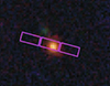 |
Fig. 1. RGB image (created using the F115W, F277W, and F444W NIRCam filters) of J0647_1045, with the NIRSpec slits overlaid (magenta rectangles). The image is centred on the coordinates of the source at RA = 101.933406, Dec = 70.198268 and is 2 arcsec on a side. |
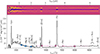 |
Fig. 2. Observed NIRSpec prism spectrum of J0647_1045. Top: 2D spectrum showing the bright Hα, Hβ, and [O III] emission. Bottom: 1D spectrum (corrected for Galactic extinction) with several identified lines labelled. The observed wavelengths are shown in μm on the top axis, while the rest-frame wavelengths are plotted in Å on the bottom axis. The NIRCam photometric fluxes in a 0.5 arcsec diameter aperture in the UV filters F115W, F150W, and F200W are shown as blue stars with the NIRCam bands shown as error bars. Optical/NIR filters F277W, F356W, and F444W are similarly shown as pink stars with error bars. |
2.2. Morphology
We modelled the galaxy’s morphology in the six NIRCam filters using GALFITM (Bamford et al. 2011; Häußler et al. 2013; Vika et al. 2013), a modified version of GALFIT 3.02 (Peng et al. 2002, 2010) that can simultaneously fit multiple bands. Since GALFITM requires pixel matched images, we modelled the 20 mas short-wavelength UV bands (F115W, F150W, and F200W) separately from the 40 mas long-wavelength optical/NIR bands (F277W, F356W, and F444W). Each set of images were fit with three models: a point source, a Sérsic profile, and a Sérsic profile with a central point source. Point spread function (PSF) models for each band were generated with WebbPSF (Perrin et al. 2012, 2014). Sigma images were derived from the weight maps provided by DJA. Object masks for background sources were created by dilating the DJA segmentation map by three pixels. Initial model parameters and sky background estimates were drawn from the DJA photometric catalogue for the MACS J0647 field.
2.3. Spectroscopy
Our spectroscopic model should account for the following features observed in LRDs: broad components in Hα and possibly Hβ, narrow line emission, a blue continuum on the UV side, and a red continuum on the optical/NIR side.
We treated the UV and optical/NIR continuum as having different origins, modelled by independent components, and simultaneously fitted emission lines with broad components added where necessary. In order to have control over the redshifts and velocity widths of individual components of each line, and properties of the two continuum components, while also accounting for the instrumental resolution, we used a custom fitting algorithm based on lmfit (Newville et al. 2014).
2.3.1. Fitting continuum and emission lines
To fit the continuum, we used two power laws with distinct power-law slopes extinguished by the Small Magellanic Cloud (SMC) dust extinction law (Gordon et al. 2003). We chose SMC extinction because, with a power-law model, the observed continuum requires a steeper attenuation than the Calzetti curve, for example, can provide (Calzetti et al. 2000). In other words, the data are not consistent with a Calzetti-attenuated power law. However, a steepened Calzetti attenuation curve (as in Salim et al. 2018) provides an equally good fit compared to the SMC extinction. The power law is of the form f(λ)∝λ−β, with β constrained to be between 0 and −3 (Bouwens et al. 2016, 2023). Even with a fixed slope dust extinction law such as the SMC, there is a strong degeneracy between the intrinsic power-law slope and the dust reddening, and therefore naturally a systematic uncertainty in the inferred extinction and/or the intrinsic slopes.
To fit emission lines, we identified a list of typical strong lines in star-forming galaxies in the wavelength region of our spectrum (∼1000−9700 Å; rest frame). We modelled each of these lines with a single Gaussian, with freely variable normalisation. We included an additional broad line for Hα (see Sect. 2.3.2). For close doublet lines, we tied the Gaussian heights based on the intrinsic line ratios; for instance, we set the [O III] 5007 to 4959 Å ratio to be 2.98 (Storey & Zeippen 2000). All the narrow line redshifts and widths were tied together. The Gaussian width was constrained to be above 100 km s−1 for narrow, and above 1000 km s−1 for broad lines (an arbitrary large value of 10 000 km s−1 was set as the maximum for both). To obtain the Gaussian width of resolution-broadened lines, we convolved the input velocity widths with the JWST prism resolution from Jakobsen et al. (2022). We scaled the resolution by a constant factor of 1.3 to account for the improved resolution for compact sources in the NIRSpec slit (see de Graaff et al. 2024; Greene et al. 2024).
We estimated fit uncertainties by running a Markov chain Monte Carlo (MCMC) algorithm using the emcee fitting module in lmfit, with initial values set to the minimised result from our lmfit fit above. Given the large number of free parameters (37 for the full fit), we used 100 walkers, 30 000 steps, and a burn-in phase of 500 steps to ensure that the chain was long enough to sample a sufficient portion of the parameter space.
2.3.2. Analysis of line widths
We conducted an analysis of emission line widths by fitting Gaussians of varying widths to individual lines. Given the low and uncertain resolution of our spectrum, we are unable to distinguish line widths below ∼1000 km s−1. Even in the highest resolution region of our spectrum towards the NIR end, we were limited to widths above ∼700 km/s. Indeed, it has been seen that the width of emission lines from point-like sources in the low resolution NIRSpec spectrum can vary by ∼1 wavelength bin (Christensen et al. 2023). Hence, we cannot realistically distinguish between lines produced by star formation (≲350 km s−1) and AGN narrow line region (NLR) emission (≲1000 km s−1). Nonetheless, we can measure broadness ≳1000 km s−1, such as from an AGN broad line region (BLR). Hα shows a clear signature of such broad emission. We tried fitting a broad component to the Hβ line as well but found no evidence of broadness and therefore did not include broad components for the other Balmer lines in the final fit (see Sect. 4.1).
3. Results
3.1. Morphology
We show our best-fit GALFIT model and residual in Fig. 3. The source appears to consist of a central component with extended irregular matter around it, visible especially in the UV bands. The best fit was obtained with a Sérsic profile and a central point source, indicating the presence of a central compact core within an extended structure: an AGN within a host galaxy, for instance. We calculated the Bayesian information criterion (BIC) for these fits, and find ΔBIC to be 2204 between the PSF and Sérsic, and 2290 between PSF and Sérsic+PSF fit for the UV bands. Similarly, ΔBIC ∼7424 between the PSF and Sérsic, and 8992 between PSF and Sérsic+PSF fit for the optical/NIR bands. This indicates that the data fit better with the inclusion of both a PSF and a Sérsic model. However, the size of the source (effective radius, re ≲ 0.17 − 0.27 kpc) is smaller than that of the PSF in the long-wavelength filters, implying that it is unresolved in the optical/NIR. The radius in the UV filters F115W, F150W, and F200W is 0.45 ± 0.06, 0.44 ± 0.05, and 0.38 ± 0.03 kpc, respectively (with GALFIT uncertainties re-scaled following Allen et al., in prep.). The change in radius may be an intrinsic feature of the morphology where the central AGN dominates towards the NIR, while the host galaxy contributes more to the continuum in the UV.
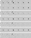 |
Fig. 3. GALFIT models and residuals in the six NIRCam bands using PSF, Sérsic, and combined Sérsic+PSF models. The PSF fit shows clear residuals, especially in the UV bands. The fit improves considerably with the addition of a Sérsic component. The best fit is obtained when both Sérsic and PSF components are used, with ΔBIC indicating a significant improvement in all bands (Sect. 3.1). |
3.2. Spectrum
The best fit to the spectrum is shown in Fig. 4. We find no appreciable velocity offset between the broad and narrow Hα lines when the Hα complex is fit separately, so we tied the narrow and broad redshifts together for the full fit. The MCMC uncertainties on broad and narrow Hα line heights and widths are shown in Fig. 5. The fit is not able to obtain a constraint on the [N II] doublet (6549 and 6585 Å) flux in the Hα complex. Setting a fixed ratio of [N II]/Hα = 1/100 (which is the expected ratio for a metallicity of ∼0.1 solar; Maiolino & Mannucci 2019) returns a poor residual, as the fit prefers a much lower ratio. Since we do not have the S/N to probe fluxes at this level, we did not include the [N II] doublet in the final fit. Instead, to place constraints on [N II] flux, we included it in the individual fit of the Hα complex (shown in the last panel of Fig. 6) and report the 1σ upper limit from the corresponding MCMC run.
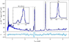 |
Fig. 4. Observed spectrum (blue step curve) with the best-fit model (dashed black curve; plotted with a finer sampling than the observed spectrum) and zoomed-in cutouts of Hβ+[O III] and Hα regions. The residuals are shown in the bottom panel. |
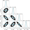 |
Fig. 5. Corner plot showing the MCMC results for heights and widths of the narrow and broad Hα components. Height is given in the same units as Fig. 4 (10−17 erg s−1 cm−2 μm−1), and velocity width is given in km s−1. |
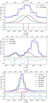 |
Fig. 6. Best fits to the [O III] and Balmer line complexes. The individual lines are indicated with coloured Gaussian curves, and their centre wavelengths are marked in the same colour in the residual panel below. The observed spectrum, best-fit, and residual curves follow the same colour scheme as Fig. 4. |
The redshift obtained for our best-fit model is 4.5319 ± 0.0001. This uncertainty includes only the statistical estimate from the MCMC. Altering model parameters results in redshifts that vary by 0.005 around the nominal value of 4.532, a consequence of the uncertainty in line widths (see Sect. 2.3.2). Moreover, a significant fraction of the residuals in our full spectrum fit are a result of the uncertainty on the dispersion function for the spectrograph. Hence, we fitted several line complexes individually to obtain accurate line fluxes, without being influenced by variations in the continuum and instrument dispersion. We show these fits in Fig. 6. The best-fit results from all the above are summarised in Table 1.
Line wavelengths and fluxes from our best-fit model.
3.3. Physical properties
Using our best-fit model, we estimated the fluxes of narrow and broad emission lines. These values are all reported in Table 1. We estimated the Balmer decrement from the narrow Hα/Hβ ratio following the prescription in Momcheva et al. (2013), finding AV = 0.9 ± 0.4, and used this to report attenuation-corrected narrow line fluxes. We also report line fluxes from He I (see Sect. 4.3) and broad Hα, corrected for extinction using an AV of 5.61 ± 0.04, from the SMC extinction on the optical/NIR power-law continuum fit.
In Table 2, we report the continuum luminosity at rest-frame 1500 Å (L1500, UV) and 5100 Å (L5100, NIR) from the UV and optical/NIR power-law fits, respectively. L1500, UV continuum luminosity was corrected by an AV of 0.38 ± 0.01 from the attenuation on the UV power-law fit. The uncertainty here is statistical, based only on the MCMC. In reality, AV is degenerate with the power-law slope, which in our fit approaches the constraint set at −3. L5100, NIR was corrected by the extinction on the optical/NIR power-law fit of AV = 5.61 ± 0.04, the same as for broad Hα line. The Balmer decrement of the broad Hα/Hβ (using the upper limit on broad Hβ) gives an AV > 4.1, which is consistent with the optical/NIR extinction. In other words, the optical/NIR extinction is sufficient to suppress a broad Hβ component (see Sect. 4.1).
Dust-corrected luminosities and inferred SFRs.
Using L1500, UV luminosity from the UV fit, and correcting for dust attenuation using the AV from the fit, we obtain an SFRUV of 12 ± 0.3 M⊙ yr−1, as indicated in Table 2. Assuming the narrow Hα luminosity arises solely from star formation, and correcting by the narrow line Balmer decrement attenuation of AV = 0.9 ± 0.4, we obtain SFR M⊙ yr−1, using the Kennicutt (1998) relation (and dividing by 1.8 to convert from Salpeter to Chabrier IMF). We also calculated SFR[OII] = 22 ± 13 M⊙ yr−1 from the [O II] doublet lines at 3728 AA using Eq. (3) of Kennicutt (1998). Using Eq. (4) of Kewley et al. (2004) results in an SFR of 11 ± 6. The latter calibration seems reasonably appropriate for galaxies at z = 4.5 (Vanderhoof et al. 2022), though the scatter is quite large. The differences in inferred SFRs may be an indication that the narrow lines, especially Hα, are not exclusively powered by star formation. We discuss this further below in Sects. 4.2 and 4.3.
The broad velocity width of the Hα line is 4300 ± 100 km s−1 (see Fig. 5). Using this velocity and the broad Hα luminosity, we estimate an SMBH mass of  M⊙ (Greene & Ho 2005; Kocevski et al. 2023). Using instead the continuum luminosity from the optical/NIR continuum at 5100 Å (L5100, NIR) results in a mass of 5 ± 0.3 × 10⁸ M⊙ (Kaspi et al. 2000; Kocevski et al. 2023). These values agree within the uncertainty range for single-epoch measurements of SMBH mass (Denney et al. 2009; Park et al. 2012; Campitiello et al. 2020). We estimate the bolometric luminosity to be 2.7 ± 0.1 × 1046 erg s−1 using the relation Lbol = 130 × LHα, broad (Stern & Laor 2012).
Assuming the narrow line flux arises only from star formation, the gas-phase metallicity (12 + log(O/H)), following the R23, O32, and O2 formulations of Sanders et al. (2024), is 7.4 ± 0.2 (or 8.7 ± 0.2 from the double-valued calibration), 7.9 ± 0.3, and 7.8 ± 0.3, respectively. This includes the intrinsic and fit uncertainties on the relation from Sanders et al. (2024), and the uncertainties on line luminosities from our MCMC estimate. These values are consistent with the need to have a very low [N II] flux to fit the Hα line as mentioned above, indicating a metallicity that may be significantly below 10% of the solar value. An estimate based on the electron temperature (Te) using the [O III] 4959, 5007 Å doublet along with Hβ and [O III] 4363 Å lines yields a similarly low metallicity of  (Pérez-Montero 2017; assuming the contribution from O+ is small compared to that from O2+). Although the density in our case may be significantly higher than that assumed in this derivation, which would result in a slightly higher metallicity.
The ionisation parameter (U) based on the sulphur and oxygen line flux ratios is relatively high. log U ∼ −2.6 from log([S III]λλ9069,9532/[S II]λλ6717,6731), and log U ∼ −2.4 from log([O III]λ5007/[O II]λλ3726,3729) following Kewley & Dopita (2002). The reason for this discrepancy is unclear, but may be related to the low metallicity and ionisation to the 3+ ions.
Finally, we estimated the gas temperature using the ratio of [O III] 4363 Å to [O III] 4959+5007 Å doublet luminosity (Nicholls et al. 2020). We obtain a value of  K (agreeing with our Te estimate above), which is the typical temperature of ionised regions in AGN environments (e.g. Larson et al. 2023). However, a substantially higher density than typically assumed may allow for a somewhat lower, though still high, temperature.
4. Diagnostics and models for the origin of the LRD phenomenon
The origin of the emission in LRDs is perhaps the biggest open question currently. Based mostly on Hα lines with widths of about 1200–4000 km/s, and on the very compact nature of these sources, AGN activity has been inferred in literature. Here we discuss the origin of the blue/UV and red/NIR continua, as well as the narrow and broad emission lines in J0647_1045, and consider several models that could reasonably fit the observed spectrum.
4.1. Broad line emission
First, we checked whether the broadness in the emission lines could arise from star-formation-related activity rather than an AGN. One possibility for line broadening is a merging system with multiple components at different redshifts (e.g. Maiolino et al. 2023). To test this, we fitted two sets of Gaussian lines each with common velocity widths < 1000 km s−1 around the Hα line region. The two sets had different redshifts, and the line centres in each were allowed to vary within ±0.01 μm of their respective redshifts. The resulting model fails to fit the broad Hα feature.
In some cases with star formation in environments where the column density of atomic hydrogen is high, Raman scattering may broaden the Balmer lines to many thousands of km/s without strong Doppler broadening (e.g. Dopita et al. 2016). Such wings can be very broad in environments with very high column densities, but are likely to be relatively weak and have Lorentzian shapes (Kokubo 2024). Given the damped Lyα absorbers with very high column densities observed in other high-redshift galaxies (Heintz et al. 2024) and the compactness of LRDs, such extreme H I columns might be present. We therefore tested an instrumentally broadened Lorentzian profile to fit the Hα line, but it did not fit the data well.
The Hα line is best-fit with an unresolved narrow component and a broad component over 4000 km/s – a velocity much higher than expected from star formation or even extreme supernova driven outflows (Fabian 2012; Baldassare et al. 2016; Davies et al. 2019). We also find no significant offset between the narrow and broad Hα components, which would be expected for an outflow. Moreover, we do not find any evidence of a broad component in the [O III] doublet at the same width and strength (relative to the narrow component) as the broad Hα component. We show the results of our MCMC analysis in Fig. 7, by which we exclude the possibility of a broad [O III] line. We therefore conclude that the most likely origin for the broad Hα line is an AGN BLR.
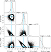 |
Fig. 7. Corner plot showing the MCMC results for broad component fits to Hβ and [O III] doublet (4959 and 5007 Å) lines. Height is given in the same units as Fig. 4 (10−17 erg s−1 cm−2 μm−1). The height of the broad component is arbitrarily small for both [O III] and Hβ. |
Curiously, we fail to find any significant broad component in Hβ (Fig. 7). This is not due to the relatively low S/N of the Hβ line compared to Hα. The Hα/Hβ ratio using the broad Hβ upper limit from the MCMC fit is ≳13. This ratio translates to an AV of ≳4.1 for an SMC extinction curve, consistent with the AV of 5.61 ± 0.04 from the optical/NIR continuum in our best-fit model, suggesting a model whereby the broad lines and red/NIR continuum are extinguished by a similar dust column. In contrast, the narrow Hα/Hβ ratio is only ∼4, which gives an AV of 0.9 ± 0.4. From our best-fit model, we obtain an AV of 0.38 ± 0.01 for the UV continuum (and a power-law slope approaching −3). In other words, the UV continuum and narrow emission lines have similar modest dust obscuration, much lower than the red/NIR continuum and broad emission lines. We conclude that there must be two distinct origins for the narrow and broad emission lines, consistent with the origins of the blue/UV and red/NIR continua, respectively.
4.2. Diagnostic diagrams
The Baldwin-Phillips-Terlevich (BPT) diagram (Baldwin et al. 1981; Kewley et al. 2013) is a common diagnostic used to separate AGNs and star-forming sources. As our best-fit model is unable to recover the [N II] flux (Sect. 3.2), we can only obtain an upper limit on the [N II]/Hα ratio. The BPT diagram (Fig. 8) suggests an extreme star formation origin for the narrow lines in J0647_1045. However, this may not be definitive since several studies find that the BPT diagram misclassifies LRDs due to their low metallicity (e.g. Harikane et al. 2023; Übler et al. 2023). The OHNO diagram (log([O III]/Hβ) vs. log([Ne III]/[O II])) has been proposed as an alternative (Kocevski et al. 2023). We plot both in Fig. 8 and compare with z ∼ 0 galaxies from the Sloan Digital Sky Survey (SDSS).
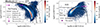 |
Fig. 8. Position of J0647_1045 on diagnostic diagrams distinguishing between emission from AGN and star formation. Left: BPT diagram of the log([N II]6585 Å/Hα) flux vs. log([O III]5007 Å/Hβ) flux of SDSS galaxies. [N II] flux is an upper limit of the 6585 Å line. The log([N II]/Hα) upper limit for this source, using only the narrow Hα component flux and the total flux (sum of the narrow and broad component fluxes), is shown by open and filled magenta diamonds, respectively. The theoretical cutoff curves for AGNs and star-forming galaxies at z = 0 from Kewley et al. (2001), Schawinski et al. (2007), and Kauffmann et al. (2003) and the redshift-dependent curve from Kewley et al. (2013) are shown as black solid, dotted, dashed, and dash-dot lines, respectively. Right: OHNO diagram of the log([Ne III]3867 Å/[O II]) vs. log([O III]5007 Å/Hβ) flux of SDSS galaxies. The curve separating AGNs and star formation from Backhaus et al. (2022) is plotted as a dashed black line. The position of this source is again marked by a magenta diamond. [O II] luminosity is the sum of the (3726, 3729 Å) doublet, modelled as a single Gaussian in our fit. In contrast, [Ne III] has been modelled as two individual Gaussians to extract the flux at ∼3867 Å separately from that at ∼3968 Å. |
The OHNO diagram also indicates a hard radiation field for the narrow lines in J0647_1045, but on the AGN side of the boundary for z = 0 galaxies. This suggests that the narrow line emission in J0647_1045 may be a combination of the star formation in the galaxy and light from the AGN NLR. Indeed, the SFR inferred from the narrow component of Hα alone is a factor of a few greater than the SFR inferred from the L1500, UV. While this could be due to the different timescales of these SF indicators, the fact that the metallicity-corrected [O II] SFR is also much lower than the Hα SFR, hints that AGN activity may contribute to the narrow line fluxes. Finally, the electron temperature we infer from the [O III] lines, as discussed in Sect. 3, is very high and may more likely be explained with a combination of a moderately high temperature and very high density, again, hinting at an AGN contribution to these lines.
4.3. He and Fe emission
We identify several He I emission lines across the spectrum. Measuring AV from He I 5877 and 7065 Å line fluxes gives a value consistent with that obtained from our optical/NIR continuum fit, and broad line Balmer decrement. This points to an AGN, rather than star formation, origin for these lines. However, as the S/N of these lines is low, we did not include broad Gaussian components to these lines in our model. Furthermore, the ratios between these lines and He I 3889 and 8446 Å are not consistent with the same AV, although He I 8446 Å may be blended with other lines ([Ne III] 3869 Å and O I 8446 Å), affecting our estimate. We also measure a flux ratio between C III] 1909 AA (obtained assuming C III] 1907/1909 = 1.53; Maseda et al. 2017; Kewley et al. 2019) and He II 1640 Å of 0.8 ± 0.2, which implies a harder radiation field than can be produced via star formation (Kewley et al. 2019). The spectrum also displays emission features at ∼9200 Å, which may be the permitted Fe II transitions at 9127, 9177, and 9202 Å (possibly blended with H I at 9230 Å), detected in many local narrow-line Seyfert 1 galaxies (e.g. Riffel et al. 2006).
4.4. Origin of the continuum
4.4.1. Thermal emission from a dust torus
Motivated by the compact-dominated nature of the morphology in the long wavelength bands, we considered whether the rest optical/NIR continuum (i.e. the red spectral side) could be modelled as direct thermal dust emission from the inner edge of an AGN torus (i.e. a blackbody curve instead of a power law). We also added variable SMC extinction, just as we did with our power-law model. This model fits the optical/NIR continuum data well, with a dust temperature of Tb ∼ 2500 K and no significant extinction required on the optical/NIR side. However, this temperature is significantly hotter than type 1 AGN dust tori, which are typically closer to 1400 K (Kishimoto et al. 2007; Hönig & Kishimoto 2010), and it is even hotter than models of carbon grain thermal sublimation temperatures, which are around 2000 K (Kobayashi et al. 2009). Moreover, if the BLR were obscured, we would expect significant dust-obscuration of the blackbody emission from the inner edge of the torus region, in contrast to the very low dust-obscuration obtained from our blackbody fit. It may be possible at certain viewing angles of the AGN for the blackbody emission from the inner dust torus to be directly transmitted to the observer without being screened by dust, but if this were the case, we would not expect to see such a large obscuration of the broad lines. Hence, while the continuum fit is good, the high temperature and inconsistency of the dust extinction with the broad Balmer lines leads us to disfavour the possibility that the optical/NIR continuum arises from thermal emission from an AGN dust torus.
The UV β slope and AV in our continuum fit are highly degenerate, but the fit favours β slopes approaching −3 (where Fλ ∝ λβ). Such an extreme blueness of the dust-corrected UV slope seems hard to explain, whether for an AGN (e.g. Hjorth et al. 2013) or for a young star-forming population (Bouwens et al. 2016). However, fixing the power-law slope to −2.7 does yield an acceptable fit. Another curious aspect of the continuum, which is beyond the scope of this paper, is the rollover of the spectrum at the Lyα break. We could not replicate this feature using dust attenuation but suggest that it may indicate Lyα damping in addition to dust attenuation (Heintz et al. 2024). Although the presence of the Lyα line in emission could be difficult to explain in that case.
4.4.2. Origin of the V-shape from an AGN core extinction curve?
It is noteworthy that the location of the break in the continuum is around 4500 Å, close to the location of the flattening in the proposed AGN core extinction curve of Gaskell et al. (2004). Is it possible that the V-shape observed in LRDs is simply the result of the flattening UV extinction curve of AGNs? To test this hypothesis, we derived an observed extinction curve for J0647_1045 by assuming the best fit red continuum AV to set the V-band normalisation of the intrinsic spectrum, and then assumed a very blue intrinsic slope (β = −2.7). We then divided the observed spectrum by this single power law and normalised by the AV. This extinction curve is shown in Fig. 9 along with the data used by Gaskell et al. (2004) to derive the AGN continuum extinction curve. The match is surprisingly good (though it must be admitted that it is difficult to differentiate this type of extinction curve from one produced by a partial covering of a high-extinction sightline). We are not too concerned with an exact match to these data here, as other assumed intrinsic normalisations and slopes will change the shape of the extinction curve somewhat. In addition, some contribution from the host galaxy must be present. There is also a range in the AGN extinction curve properties derived for other AGNs with slightly different break wavelengths and UV slopes (e.g. Gaskell 2017). However, overall the match is similar, showing strong reddening up to about 4000 Å and then a much flatter extinction in the blue/UV. These flat UV extinction curves have been argued to be the product of the thermal sublimation of smaller grains by the AGN UV and X-ray emission. However, it is unclear why the AGN would destroy small grains deep into the torus, and in that case, the extinction curve would only be UV-flat in regions with relatively modest UV extinctions (i.e. with AUV ≲ 1). For this reason, we would expect the overall extinction curve to be UV-flat only for a small subset of AGNs viewed at specific angles and with modest extinctions. This cannot be the case for J0647_1045 or most LRDs. Hence, despite the notable agreement between the V-shaped SED phenomenon in LRDs and a single power-law fit with AGN-core extinction, we do not currently favour this explanation.
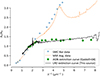 |
Fig. 9. Extinction curve of J0647_1045 assuming a single power-law intrinsic spectrum. The AGN core emission extinction data of Gaskell et al. (2004) are shown for comparison alongside the Milky Way (MW) average extinction from Gordon et al. (2009) and the SMC bar extinction data from Gordon et al. (2003). The close match to the Gaskell et al. (2004) curve data indicates that the observed V-shaped continuum of the LRDs could be produced by a single power-law continuum with a peculiar AGN extinction. |
4.4.3. Other origins of the V-shape
The apparently V-shaped SEDs of LRDs have been suggested to be due to an AGN observed in dust-obscured direct emission and low-extinction scattered emission (Labbe et al. 2023), or obscured star formation with the blue component due to direct AGN emission (Kocevski et al. 2023). Another possibility considered is a partial coverer, with a small fraction of low-extinction emission (A. Goulding, priv. comm.). In all these cases, the blue light would be expected to be dominated by a point source, possibly compatible with the imaging data for this source. However, the Balmer decrement should also be small for the broad lines for all these hypotheses, since the dust obscuration should not affect the scattered broad lines very much. Since we do not detect broad Hβ, none of these hypotheses seem compatible with the data in our case. A Balmer break was also proposed (Labbe et al. 2023) but seems unlikely to produce the observed features here.
4.5. Are we observing the AGN core directly through a dust screen?
One possible interpretation of the LRD phenomenon is a type 2 AGN in a star-forming host galaxy. While at lower redshifts most AGNs are in relatively metal-rich hosts, as we go to high redshifts, the host galaxies will be more metal poor and therefore also more dust poor. It is not inconsistent with the existing data to argue that the LRDs may be type 2 AGNs in low-metallicity hosts, viewed directly through their obscuring ‘dusty torus’. At lower redshifts, the metallicity is closer to the solar value and the gas-to-dust ratio is close to Galactic. In a scenario where the total gas column density through the torus is above  , the typical AV will be 50 − 500 magnitudes at Galactic gas-to-dust ratios, and these AGNs would only be detected along their lowest extinction orientations at optical/NIR wavelengths.
However, at z > 4, where the host galaxy metallicity may be 1–10% of the solar value, the AV could be only a few magnitudes, since the dust-to-gas ratio is likely to be 20–1000 times lower than the Galactic value at these metallicities (Konstantopoulou et al. 2023). This would allow these AGNs to be detected directly through their dust tori. In this scenario, we would expect low metallicities to be typical for LRDs. In the very lowest metallicity cases, strong molecular hydrogen absorption bands would be expected in the UV; however, in almost all cases, the Lyman-Werner bands will not be detectable due to the suppression of the UV flux at even very low metallicity and bluewards of Lyα by intergalactic H I at high redshifts.
Whether LRDs really are the direct detection of the elusive population of type 2 AGNs at high redshifts could be tested based on number counts, X-ray limits, and spectra. The current lack of X-ray detections (Matthee et al. 2024; Furtak et al. 2024) is already somewhat problematic for an AGN scenario, and seems to require lower-mass black holes and super-Eddington accretion (Greene et al. 2024; Fujimoto et al. 2022).
Photoelectric absorption through the torus could significantly suppress the X-ray emission even in the low metallicity scenario. For example, for a spectrum taken through gas clouds with, for example, 2% solar metallicity, which corresponds to a dust-to-gas ratio of 10−5 (Konstantopoulou et al. 2023), and assuming an AV = 6, would require an actual (not equivalent) hydrogen column density of ∼1025 cm−2. Soft X-rays will still be significantly absorbed below about 1 keV in the observed frame for systems at z ∼ 5. However, for these high-redshift systems, harder X-rays should still be detectable. In this hypothesis, the sources are unlikely to be Compton thick since the dust-to-gas ratios inferred would have to be well below expectations for the sort of metallicities these galaxies seem to have.
4.6. Comparison with other LRDs
In Fig. 10, we plot the bolometric luminosity against SMBH mass for J0647_1045 and other LRDs from the literature. Some of these works have corrected their estimates for dust attenuation (e.g. Greene et al. 2024), while others (e.g. Matthee et al. 2024) have not corrected for dust. For a fair comparison with such cases, we plot the measurements for our source with Balmer and AGN dust correction, and with no dust correction. As can be seen, if AGN dust correction is applied, J0647_1045 is among the most extreme LRDs detected so far.
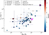 |
Fig. 10. SMBH mass and bolometric luminosity of J0647_1045 in comparison with measurements for other LRDs from the literature (Harikane et al. 2023; Kocevski et al. 2023; Kokorev et al. 2023; Larson et al. 2023; Furtak et al. 2024; Greene et al. 2024; Maiolino et al. 2023; Matthee et al. 2024). The symbols are as indicated in the legend, and the colour-scale represents redshift. The filled magenta star shows SMBH mass and Lbol estimates for our source, derived from a broad Hα line using a dust correction of AV = 5.61 ± 0.04, corresponding to the AGN extinction from our model. The empty magenta star shows these properties corrected by AV = 0.9 ± 0.4, which corresponds to Balmer attenuation. The empty black star shows measurements for our source with no dust correction applied. |
4.7. Future avenues
There are several directions to explore the LRD phenomenon and its connection to the obscured AGN population. One possibility is to conduct large JWST surveys targeting this population, which can help set constraints on the AGN number counts in the early Universe. Preliminary efforts in this direction have already proven promising (e.g. Greene et al. 2024; Maiolino et al. 2023; Harikane et al. 2023). In addition, deeper data can reveal if there are broad components in other emission lines besides Balmer lines, or at least set limits on the strength of the AGN and the extent of dust extinction. High resolution spectroscopy will identify which emission lines are AGN- or star-formation-powered, and will also resolve doublets for better estimates of line luminosities, and in turn physical properties (e.g. Kocevski et al. 2023). In particular, accurate estimates of the metallicities of LRDs could be extremely informative. IFS data, as in Parlanti et al. (2024), would help map the relative spatial extent of broad Hα and narrow [O III]. Furthermore, since time variable measurements provide much more accurate SMBH properties than single-epoch derivations, observing LRDs at intervals to detect potential variability over time would provide better constraints on the AGN powering these systems.
As a new class of objects, LRDs would benefit from their own template for SED fitting so that we can group similar objects under a new, more appropriate classification. The NIRSpec spectrum presented here for J0647_1045 has very good S/N and may be used as a template2 for future LRD samples.
5. Conclusions
We have presented the JWST NIRCam images and NIRSpec spectrum of J0647_1045, a gravitationally lensed compact source with an unusual V-shaped continuum. We fitted both the morphology and spectrum using various models, describing outflows, mergers, dust-obscured star formation, AGN activity, and AGN dust torus emission. The best fit to the spectrum was obtained by assuming two distinct components for the UV and optical/NIR sides of the spectrum, with different power-law slopes and dust extinctions. We also find that while nearly all emission lines fit well with a Gaussian with a width of less than 1000 km s−1, the Hα line shows evidence of AGN-broadening with a velocity width of 4300 ± 100 km s−1, indicating that J0647_1045 is an LRD with one of the highest inferred SMBH masses measured so far. Our modelling favours a scenario in which the UV continuum arises from a star-forming region with low obscuration, the narrow emission lines arise from star formation and/or possibly an AGN NLR, and the optical/NIR continuum and broad line emission arise from the AGN and its surrounding BLR. The morphology, extended in the UV and more compact towards the NIR, supports the domination of extended star formation in the UV and compact AGN emission towards the NIR. We therefore conclude that the system is a highly obscured AGN within a less obscured star-forming host galaxy. The exhibition of features of both AGNs (broad Hα line) and star formation (spatially extended emission) in J0647_1045 may indicate the current stage of evolution of a young AGN that will eventually grow and dominate the host galaxy flux (Fujimoto et al. 2022; Matthee et al. 2024). LRDs in general may evolve into the AGN-dominated, bright blue quasars we see at lower redshifts, requiring a black hole mass increase of nearly two orders of magnitude. This would entail near-Eddington or super-Eddington accretion rates or mergers over the next few billion years. We propose that LRDs may be low-metallicity type 2 AGNs with very low dust-to-gas ratios viewed ‘through’ their dust torus, giving rise to the direct detectability of their AGN in rest-frame red and NIR light.
Acknowledgments
The data products presented herein were retrieved from the DAWN JWST Archive (DJA), an initiative of the Cosmic Dawn Center. The Cosmic Dawn Center is funded by the Danish National Research Foundation under grant DNRF140. M.K. was supported by the ANID BASAL project FB210003.
References
- Backhaus, B. E., Trump, J. R., Cleri, N. J., et al. 2022, ApJ, 926, 161 [NASA ADS] [CrossRef] [Google Scholar]
- Baldassare, V. F., Reines, A. E., Gallo, E., et al. 2016, ApJ, 829, 57 [NASA ADS] [CrossRef] [Google Scholar]
- Baldwin, J. A., Phillips, M. M., & Terlevich, R. 1981, PASP, 93, 5 [Google Scholar]
- Bamford, S. P., Häußler, B., Rojas, A., et al. 2011, ASP Conf. Ser., 442, 479 [NASA ADS] [Google Scholar]
- Barro, G., Pérez-González, P. G., Kocevski, D. D., et al. 2024, ApJ, 963, 128 [CrossRef] [Google Scholar]
- Bouwens, R., Aravena, M., Decarli, R., et al. 2016, ApJ, 833, 72 [NASA ADS] [CrossRef] [Google Scholar]
- Bouwens, R. J., Stefanon, M., Brammer, G., et al. 2023, MNRAS, 523, 1036 [NASA ADS] [CrossRef] [Google Scholar]
- Brammer, G. 2023, https://doi.org/10.5281/zenodo.8233475 [Google Scholar]
- Bromm, V., & Loeb, A. 2003, ApJ, 596, 34 [Google Scholar]
- Calzetti, D., Armus, L., Bohlin, R. C., et al. 2000, ApJ, 533, 682 [NASA ADS] [CrossRef] [Google Scholar]
- Campitiello, S., Celotti, A., Ghisellini, G., & Sbarrato, T. 2020, A&A, 640, A39 [NASA ADS] [CrossRef] [EDP Sciences] [Google Scholar]
- Chabrier, G. 2003, PASP, 115, 763 [Google Scholar]
- Chantavat, T., Chongchitnan, S., & Silk, J. 2023, MNRAS, 522, 3256 [NASA ADS] [CrossRef] [Google Scholar]
- Christensen, L., Jakobsen, P., Willott, C., et al. 2023, A&A, 680, A82 [NASA ADS] [CrossRef] [EDP Sciences] [Google Scholar]
- Davies, R. L., Schreiber, N. M. F., Übler, H., et al. 2019, ApJ, 873, 122 [NASA ADS] [CrossRef] [Google Scholar]
- de Graaff, A., Rix, H.-W., Carniani, S., et al. 2024, A&A, 684, A87 [NASA ADS] [CrossRef] [EDP Sciences] [Google Scholar]
- Denney, K. D., Peterson, B. M., Dietrich, M., Vestergaard, M., & Bentz, M. C. 2009, ApJ, 692, 246 [NASA ADS] [CrossRef] [Google Scholar]
- Dopita, M. A., Nicholls, D. C., Sutherland, R. S., Kewley, L. J., & Groves, B. A. 2016, ApJ, 824, L13 [NASA ADS] [CrossRef] [Google Scholar]
- Ebeling, H., Edge, A. C., Mantz, A., et al. 2010, MNRAS, 407, 83 [NASA ADS] [CrossRef] [Google Scholar]
- Fabian, A. C. 2012, ARA&A, 50, 455 [Google Scholar]
- Fujimoto, S., Brammer, G. B., Watson, D., et al. 2022, Nature, 604, 261 [NASA ADS] [CrossRef] [Google Scholar]
- Fujimoto, S., Arrabal Haro, P., Dickinson, M., et al. 2023, ApJ, 949, L25 [NASA ADS] [CrossRef] [Google Scholar]
- Furtak, L. J., Labbé, I., Zitrin, A., et al. 2024, Nature, 628, 57 [NASA ADS] [CrossRef] [Google Scholar]
- Gaskell, C. 2017, MNRAS, 467, 226 [Google Scholar]
- Gaskell, C. M., Goosmann, R. W., Antonucci, R. R. J., & Whysong, D. H. 2004, ApJ, 616, 147 [NASA ADS] [CrossRef] [Google Scholar]
- Gordon, K. D., Clayton, G. C., Misselt, K. A., Landolt, A. U., & Wolff, M. J. 2003, ApJ, 594, 279 [NASA ADS] [CrossRef] [Google Scholar]
- Gordon, K. D., Cartledge, S., & Clayton, G. C. 2009, ApJ, 705, 1320 [NASA ADS] [CrossRef] [Google Scholar]
- Green, G. 2018, J. Open Source Softw., 3, 695 [NASA ADS] [CrossRef] [Google Scholar]
- Greene, J. E., & Ho, L. C. 2005, ApJ, 630, 122 [NASA ADS] [CrossRef] [Google Scholar]
- Greene, J. E., Labbe, I., Goulding, A. D., et al. 2024, ApJ, 964, 39 [CrossRef] [Google Scholar]
- Harikane, Y., Zhang, Y., Nakajima, K., et al. 2023, ApJ, 959, 39 [NASA ADS] [CrossRef] [Google Scholar]
- Häußler, B., Bamford, S. P., Vika, M., et al. 2013, MNRAS, 430, 330 [Google Scholar]
- Heintz, K. E., Watson, D., Brammer, G., et al. 2024, Science, 384, 890 [NASA ADS] [CrossRef] [Google Scholar]
- Hjorth, J., Vreeswijk, P. M., Gall, C., & Watson, D. 2013, ApJ, 768, 173 [NASA ADS] [CrossRef] [Google Scholar]
- Hönig, S. F., & Kishimoto, M. 2010, A&A, 523, A27 [NASA ADS] [CrossRef] [EDP Sciences] [Google Scholar]
- Horne, K. 1986, PASP, 98, 609 [Google Scholar]
- Jakobsen, P., Ferruit, P., Alves de Oliveira, C., et al. 2022, A&A, 661, A80 [NASA ADS] [CrossRef] [EDP Sciences] [Google Scholar]
- Kaspi, S., Smith, P. S., Netzer, H., et al. 2000, ApJ, 533, 631 [Google Scholar]
- Kauffmann, G., Heckman, T. M., Tremonti, C., et al. 2003, MNRAS, 346, 1055 [Google Scholar]
- Kennicutt, R. C. 1998, ARA&A, 36, 189 [NASA ADS] [CrossRef] [Google Scholar]
- Kewley, L. J., & Dopita, M. A. 2002, ApJS, 142, 35 [Google Scholar]
- Kewley, L. J., Dopita, M. A., Sutherland, R. S., Heisler, C. A., & Trevena, J. 2001, ApJ, 556, 121 [Google Scholar]
- Kewley, L. J., Geller, M. J., & Jansen, R. A. 2004, AJ, 127, 2002 [Google Scholar]
- Kewley, L. J., Maier, C., Yabe, K., et al. 2013, ApJ, 774, L10 [Google Scholar]
- Kewley, L. J., Nicholls, D. C., & Sutherland, R. S. 2019, ARA&A, 57, 511 [Google Scholar]
- Kishimoto, M., Hoenig, S. F., Beckert, T., & Weigelt, G. 2007, A&A, 476, 713 [NASA ADS] [CrossRef] [EDP Sciences] [Google Scholar]
- Kobayashi, H., Watanabe, S. I., Kimura, H., & Yamamoto, T. 2009, Icarus, 201, 395 [NASA ADS] [CrossRef] [Google Scholar]
- Kocevski, D. D., Onoue, M., Inayoshi, K., et al. 2023, ApJ, 954, L4 [NASA ADS] [CrossRef] [Google Scholar]
- Kokorev, V., Fujimoto, S., Labbe, I., et al. 2023, ApJ, 957, L7 [NASA ADS] [CrossRef] [Google Scholar]
- Kokubo, M. 2024, MNRAS, 529, 2131 [NASA ADS] [CrossRef] [Google Scholar]
- Konstantopoulou, C., De Cia, A., Krogager, J.-K., et al. 2023, A&A, 674, C1 [NASA ADS] [CrossRef] [EDP Sciences] [Google Scholar]
- Labbe, I., Greene, J. E., Bezanson, R., et al. 2023, ArXiv e-prints [arXiv:2306.07320] [Google Scholar]
- Larson, R. L., Finkelstein, S. L., Kocevski, D. D., et al. 2023, ApJ, 953, L29 [NASA ADS] [CrossRef] [Google Scholar]
- Maiolino, R., & Mannucci, F. 2019, A&ARv, 27, 3 [Google Scholar]
- Maiolino, R., Scholtz, J., Curtis-Lake, E., et al. 2023, ArXiv e-prints [arXiv:2308.01230] [Google Scholar]
- Maseda, M. V., Brinchmann, J., Franx, M., et al. 2017, A&A, 608, A4 [NASA ADS] [CrossRef] [EDP Sciences] [Google Scholar]
- Matthee, J., Naidu, R. P., Brammer, G., et al. 2024, ApJ, 963, 129 [NASA ADS] [CrossRef] [Google Scholar]
- Momcheva, I. G., Lee, J. C., Ly, C., et al. 2013, AJ, 145, 47 [NASA ADS] [CrossRef] [Google Scholar]
- Natarajan, P., Pacucci, F., Ricarte, A., et al. 2024, ApJ, 960, L1 [NASA ADS] [CrossRef] [Google Scholar]
- Newville, M., Stensitzki, T., Allen, D. B., & Ingargiola, A. 2014, https://doi.org/10.5281/zenodo.11813 [Google Scholar]
- Nicholls, D. C., Kewley, L. J., Sutherland, R. S., et al. 2020, PASP, 132, 033001 [NASA ADS] [CrossRef] [Google Scholar]
- Ohkubo, T., Nomoto, K., Umeda, H., Yoshida, N., & Tsuruta, S. 2009, ApJ, 706, 1184 [NASA ADS] [CrossRef] [Google Scholar]
- Onoue, M., Inayoshi, K., Ding, X., et al. 2023, ApJ, 942, L17 [NASA ADS] [CrossRef] [Google Scholar]
- Park, D., Woo, J. H., Treu, T., et al. 2012, ApJ, 747, 30 [CrossRef] [Google Scholar]
- Parlanti, E., Carniani, S., Übler, H., et al. 2024, A&A, 684, A24 [NASA ADS] [CrossRef] [EDP Sciences] [Google Scholar]
- Peng, C. Y., Ho, L. C., Impey, C. D., & Rix, H.-W. 2002, AJ, 124, 266 [Google Scholar]
- Peng, C. Y., Ho, L. C., Impey, C. D., & Rix, H. W. 2010, AJ, 139, 2097 [Google Scholar]
- Pérez-Montero, E. 2017, PASP, 129, 043001 [CrossRef] [Google Scholar]
- Perrin, M. D., Soummer, R., Elliott, E. M., et al. 2012, Proc. SPIE, 8442, 84423D [NASA ADS] [CrossRef] [Google Scholar]
- Perrin, M. D., Sivaramakrishnan, A., Lajoie, C.-P., et al. 2014, Proc. SPIE, 9143, 91433X [NASA ADS] [CrossRef] [Google Scholar]
- Planck Collaboration VI. 2020, A&A, 641, A6 [NASA ADS] [CrossRef] [EDP Sciences] [Google Scholar]
- Riffel, R., Rodríguez-Ardila, A., & Pastoriza, M. G. 2006, A&A, 457, 61 [NASA ADS] [CrossRef] [EDP Sciences] [Google Scholar]
- Salim, S., Boquien, M., & Lee, J. C. 2018, ApJ, 859, 11 [Google Scholar]
- Sanders, R. L., Shapley, A. E., Topping, M. W., Reddy, N. A., & Brammer, G. B. 2024, ApJ, 962, 24 [NASA ADS] [CrossRef] [Google Scholar]
- Schawinski, K., Thomas, D., Sarzi, M., et al. 2007, MNRAS, 382, 1415 [Google Scholar]
- Schneider, R., Valiante, R., Trinca, A., et al. 2023, MNRAS, 526, 3250 [NASA ADS] [CrossRef] [Google Scholar]
- Stern, J., & Laor, A. 2012, MNRAS, 423, 600 [NASA ADS] [CrossRef] [Google Scholar]
- Storey, P. J., & Zeippen, C. J. 2000, MNRAS, 312, 813 [NASA ADS] [CrossRef] [Google Scholar]
- Trinca, A., Schneider, R., Valiante, R., et al. 2022, 44th COSPAR Scientific Assembly, held 16–24 July, 44, 1828 [Google Scholar]
- Übler, H., Maiolino, R., Curtis-Lake, E., et al. 2023, A&A, 677, A145 [NASA ADS] [CrossRef] [EDP Sciences] [Google Scholar]
- Vanderhoof, B. N., Faisst, A. L., Shen, L., et al. 2022, MNRAS, 511, 1303 [NASA ADS] [CrossRef] [Google Scholar]
- Vika, M., Bamford, S. P., Häußler, B., et al. 2013, MNRAS, 435, 623 [NASA ADS] [CrossRef] [Google Scholar]
- Wang, F., Yang, J., Fan, X., et al. 2021, ApJ, 907, L1 [Google Scholar]
All Tables
All Figures
|
Fig. 1. RGB image (created using the F115W, F277W, and F444W NIRCam filters) of J0647_1045, with the NIRSpec slits overlaid (magenta rectangles). The image is centred on the coordinates of the source at RA = 101.933406, Dec = 70.198268 and is 2 arcsec on a side. |
| In the text | |
|
Fig. 2. Observed NIRSpec prism spectrum of J0647_1045. Top: 2D spectrum showing the bright Hα, Hβ, and [O III] emission. Bottom: 1D spectrum (corrected for Galactic extinction) with several identified lines labelled. The observed wavelengths are shown in μm on the top axis, while the rest-frame wavelengths are plotted in Å on the bottom axis. The NIRCam photometric fluxes in a 0.5 arcsec diameter aperture in the UV filters F115W, F150W, and F200W are shown as blue stars with the NIRCam bands shown as error bars. Optical/NIR filters F277W, F356W, and F444W are similarly shown as pink stars with error bars. |
| In the text | |
|
Fig. 3. GALFIT models and residuals in the six NIRCam bands using PSF, Sérsic, and combined Sérsic+PSF models. The PSF fit shows clear residuals, especially in the UV bands. The fit improves considerably with the addition of a Sérsic component. The best fit is obtained when both Sérsic and PSF components are used, with ΔBIC indicating a significant improvement in all bands (Sect. 3.1). |
| In the text | |
|
Fig. 4. Observed spectrum (blue step curve) with the best-fit model (dashed black curve; plotted with a finer sampling than the observed spectrum) and zoomed-in cutouts of Hβ+[O III] and Hα regions. The residuals are shown in the bottom panel. |
| In the text | |
|
Fig. 5. Corner plot showing the MCMC results for heights and widths of the narrow and broad Hα components. Height is given in the same units as Fig. 4 (10−17 erg s−1 cm−2 μm−1), and velocity width is given in km s−1. |
| In the text | |
|
Fig. 6. Best fits to the [O III] and Balmer line complexes. The individual lines are indicated with coloured Gaussian curves, and their centre wavelengths are marked in the same colour in the residual panel below. The observed spectrum, best-fit, and residual curves follow the same colour scheme as Fig. 4. |
| In the text | |
|
Fig. 7. Corner plot showing the MCMC results for broad component fits to Hβ and [O III] doublet (4959 and 5007 Å) lines. Height is given in the same units as Fig. 4 (10−17 erg s−1 cm−2 μm−1). The height of the broad component is arbitrarily small for both [O III] and Hβ. |
| In the text | |
|
Fig. 8. Position of J0647_1045 on diagnostic diagrams distinguishing between emission from AGN and star formation. Left: BPT diagram of the log([N II]6585 Å/Hα) flux vs. log([O III]5007 Å/Hβ) flux of SDSS galaxies. [N II] flux is an upper limit of the 6585 Å line. The log([N II]/Hα) upper limit for this source, using only the narrow Hα component flux and the total flux (sum of the narrow and broad component fluxes), is shown by open and filled magenta diamonds, respectively. The theoretical cutoff curves for AGNs and star-forming galaxies at z = 0 from Kewley et al. (2001), Schawinski et al. (2007), and Kauffmann et al. (2003) and the redshift-dependent curve from Kewley et al. (2013) are shown as black solid, dotted, dashed, and dash-dot lines, respectively. Right: OHNO diagram of the log([Ne III]3867 Å/[O II]) vs. log([O III]5007 Å/Hβ) flux of SDSS galaxies. The curve separating AGNs and star formation from Backhaus et al. (2022) is plotted as a dashed black line. The position of this source is again marked by a magenta diamond. [O II] luminosity is the sum of the (3726, 3729 Å) doublet, modelled as a single Gaussian in our fit. In contrast, [Ne III] has been modelled as two individual Gaussians to extract the flux at ∼3867 Å separately from that at ∼3968 Å. |
| In the text | |
|
Fig. 9. Extinction curve of J0647_1045 assuming a single power-law intrinsic spectrum. The AGN core emission extinction data of Gaskell et al. (2004) are shown for comparison alongside the Milky Way (MW) average extinction from Gordon et al. (2009) and the SMC bar extinction data from Gordon et al. (2003). The close match to the Gaskell et al. (2004) curve data indicates that the observed V-shaped continuum of the LRDs could be produced by a single power-law continuum with a peculiar AGN extinction. |
| In the text | |
|
Fig. 10. SMBH mass and bolometric luminosity of J0647_1045 in comparison with measurements for other LRDs from the literature (Harikane et al. 2023; Kocevski et al. 2023; Kokorev et al. 2023; Larson et al. 2023; Furtak et al. 2024; Greene et al. 2024; Maiolino et al. 2023; Matthee et al. 2024). The symbols are as indicated in the legend, and the colour-scale represents redshift. The filled magenta star shows SMBH mass and Lbol estimates for our source, derived from a broad Hα line using a dust correction of AV = 5.61 ± 0.04, corresponding to the AGN extinction from our model. The empty magenta star shows these properties corrected by AV = 0.9 ± 0.4, which corresponds to Balmer attenuation. The empty black star shows measurements for our source with no dust correction applied. |
| In the text | |
Current usage metrics show cumulative count of Article Views (full-text article views including HTML views, PDF and ePub downloads, according to the available data) and Abstracts Views on Vision4Press platform.
Data correspond to usage on the plateform after 2015. The current usage metrics is available 48-96 hours after online publication and is updated daily on week days.
Initial download of the metrics may take a while.