| Issue |
A&A
Volume 698, June 2025
|
|
|---|---|---|
| Article Number | A49 | |
| Number of page(s) | 19 | |
| Section | Stellar structure and evolution | |
| DOI | https://doi.org/10.1051/0004-6361/202453533 | |
| Published online | 28 May 2025 | |
Asteroseismic predictions for a massive main-sequence merger product
1
Heidelberg Institute for Theoretical Studies, Schloss-Wolfsbrunnenweg 35, 69118 Heidelberg, Germany
2
Universität Heidelberg, Department of Physics and Astronomy, Im Neuenheimer Feld 226, 69120 Heidelberg, Germany
3
Zentrum für Astronomie, Astronomisches Rechen-Institut (ZAH/ARI), Heidelberg University, Mönchhofstr. 12-14, 69120 Heidelberg, Germany
4
Zentrum für Astronomie, Landessternwarte (ZAH/LSW), Heidelberg University, Königstuhl 12, 69117 Heidelberg, Germany
5
Institute of Astronomy, KU Leuven, Celestijnenlaan 200D, 3001 Leuven, Belgium
6
Department of Astrophysics, IMAPP, Radboud University Nijmegen, PO Box 9010, 6500 GL Nijmegen, The Netherlands
7
Max Planck Institute for Astronomy, Königstuhl 17, 69117 Heidelberg, Germany
⋆ Corresponding author: This email address is being protected from spambots. You need JavaScript enabled to view it.
Received:
19
December
2024
Accepted:
7
April
2025
Abstract
The products of stellar mergers between two massive main-sequence stars appear as seemingly normal main-sequence stars after a phase of thermal relaxation, if not for certain peculiarities. These peculiarities, such as strong magnetic fields, chemically enriched surfaces, rejuvenated cores, and masses above the main-sequence turnoff mass, have been proposed to indicate merger or mass accretion origins. Since these peculiarities are not limited to the merger product's surface, we use asteroseismology to predict how the differences in the internal structure of a merger product and a genuine single star manifest via properties of non-radial stellar pulsations. We use the result of a 3D (magneto)hydrodynamic simulation of a stellar merger between a 9 and an 8 M⊙ main-sequence star, which was mapped to 1D and evolved through the main sequence. We compare the predicted pressure and gravity modes for the merger product model with those predicted for a corresponding genuine single-star model. The pressure-mode frequencies are consistently lower for the merger product than for the genuine single star, and the differences between them are more than a thousand times larger than the current best observational uncertainties for measured mode frequencies of this kind. Even though the absolute differences in gravity-mode period spacings vary in value and sign throughout the main-sequence life of both stars, they, too, are larger than the current best observational uncertainties for such long-period modes. This, combined with additional variability in the merger product's period spacing patterns, shows the potential of identifying merger products in future-forward modelling. We also attempt to replicate the merger product's structure using three widely applied 1D merger prescriptions and repeat the asteroseismic analysis. Although none of the 1D prescriptions reproduces the entire merger product's structure, we conclude that the prescription with shock heating shows the highest potential, provided that it can be calibrated on binary-evolution-driven 3D merger simulations. Our work focuses on a particular kind of massive main-sequence merger and should be expanded to encompass the various possible merger product structures predicted to exist in the Universe.
Key words: asteroseismology / methods: numerical / binaries: general / stars: evolution / stars: massive / stars: oscillations
© The Authors 2025
 Open Access article, published by EDP Sciences, under the terms of the Creative Commons Attribution License (https://creativecommons.org/licenses/by/4.0), which permits unrestricted use, distribution, and reproduction in any medium, provided the original work is properly cited.
This article is published in open access under the Subscribe to Open model. This email address is being protected from spambots. You need JavaScript enabled to view it. to support open access publication.
1. Introduction
When two massive main-sequence (MS) stars (i.e. intermediate- and high-mass stars, with initial masses Mi of 1.3 M⊙≲Mi≲8 M⊙ and Mi≳8 M⊙, respectively) merge, they form a new MS star with potentially peculiar properties. For example, it has been proposed and shown that such mergers produce strong, large-scale surface magnetic fields in the resulting merger products (Ferrario et al. 2009; Wickramasinghe et al. 2014; Schneider et al. 2019; Ryu et al. 2025). Should it indeed be true that such merger products are slow rotators, as found in Schneider et al. (2019, 2020), they are a natural explanation for the blue MS band in young stellar clusters (Wang et al. 2022). MS merger products can also appear as blue stragglers in star clusters (Rasio 1995; Sills et al. 1997, 2001; Mapelli et al. 2006; Glebbeek et al. 2008; Ferraro et al. 2012; Schneider et al. 2015). Further along their evolution, MS merger products can appear as red stragglers in a population of red supergiants, which can lead to cluster age underestimations of ∼60% (Britavskiy et al. 2019).
Despite these peculiarities, it is currently not straightforward to distinguish massive MS merger products from genuine single MS stars based on surface diagnostics alone. If one or more unambiguous distinguishing features of merger products were to be found, they could be used to confirm, for example, their slow-rotation hypothesis. To find such distinguishing features, we ought to go beyond the stars’ surface diagnostics and assess any differences in their internal structure as predicted by merger simulations (Lombardi et al. 1996; Sandquist et al. 1997; Sills et al. 2001; Freitag & Benz 2005; Dale & Davies 2006; Glebbeek et al. 2013; Schneider et al. 2019; Ballone et al. 2023). Asteroseismology has proven to be the ideal tool to do so (see e.g. Hekker & Christensen-Dalsgaard 2017; Aerts 2021; Kurtz 2022; Bowman 2023 for recent reviews). Bellinger et al. (2024) and Henneco et al. (2024a) made asteroseismic predictions to identify distinguishing features of different physical object classes appearing as blue supergiants, including post-MS merger products. Wagg et al. (2024) used asteroseismic predictions of rejuvenated MS accretors to assess whether they can be distinguished from MS stars with the same mass that have not accreted matter. They conclude that the effects of accretion on the accretor's internal structure produce a measurable difference in its asteroseismic signal compared to that of regular MS stars.
An obvious prerequisite for using asteroseismology is that the stars show pulsations. This is indeed the case for many massive MS stars. Thanks to space-based asteroseismic observations with, for example, Convection, Rotation and planetary Transits (CoRoT, Auvergne et al. 2009), Kepler/K2 (Koch et al. 2010), and the Transiting Exoplanet Survey Satellite (TESS, Ricker et al. 2016) a wealth of MS pulsators have been found and characterised (Aerts 2021; Kurtz 2022). Fewer detections are currently available for stars with masses above roughly 8 M⊙, which is the mass regime this work focuses on. Yet, the future looks bright thanks to the ongoing TESS and upcoming PLAnetary Transits and Oscillations of stars (PLATO, Rauer et al. 2025) missions. Stars in this mass regime have also been shown to exhibit low-frequency stochastic variability, for which the origin is currently still being debated (e.g. Bowman et al. 2019, 2024; Anders et al. 2023; Ma et al. 2024). Mode excitation calculations (e.g. Bouabid et al. 2013; Moravveji 2016; Szewczuk & Daszyńska-Daszkiewicz 2017) also predict massive MS stars to exhibit a variety of pulsations. Moreover, it is becoming increasingly clear that our current excitation theories tend to under-predict the number of excited linear modes (e.g. Moravveji 2016; Rehm et al. 2024), as well as the actually observed modes in stars (e.g. Balona 2024; Hey & Aerts 2024). Additional mode excitation theories for MS stars, such as non-linear resonant mode coupling (Guo et al. 2022; Van Beeck et al. 2024), are currently not included in mode instability predictions while such modes were found to be common among B-type pulsators (Van Beeck et al. 2021). Finally, tidal excitation (Guo 2021, for a review) should not be ignored given the high fraction of massive stars in close binaries (Sana et al. 2012).
This work consists of two parts. In the first part, we determine whether it is possible to distinguish a massive MS merger product from a genuine single MS star following a quasi-identical evolution in the Hertzsprung-Russell diagram (HRD). To do so, we make use of the 3D magnetohydrodynamic (MHD) merger product model from Schneider et al. (2019), which we map to 1D following Schneider et al. (2020) to follow its post-merger evolution. In the second part, we repeat the first part's analysis, using 1D merger prescriptions instead of a 3D merger product model. 3D simulations of stellar mergers are computationally expensive, and hence, a limited number of 3D merger models are available. Multiple 1D merger prescriptions have been developed in an attempt to alleviate this problem. Contrary to 3D simulations, these 1D merger prescriptions do not model the merger phase itself but instead predict the structure of the merger product based on those of the binary components before the merger. Therefore, in the second part of this work, we investigate whether using three of these 1D merger prescriptions (entropy sorting, Python Make Me A Massive Star, and fast accretion) results in similarly structured merger product models as the one resulting from the 3D simulation. We then assess to what extent any asteroseismic differences between the MS merger product and its corresponding genuine single star found in the first part of this work are recovered with the 1D merger models.
The structure of this work is as follows. In Sect. 2, we provide the basic concepts and diagnostics of asteroseismology necessary for the analysis and discussion. Section 3 covers the methods used to create merger products, evolve them and their genuine single-star counterparts, and predict their pulsations. We show and discuss our results in Sect. 4, and the conclusions can be found in Sect. 5.
2. Asteroseismic diagnostics
This section gives a brief overview of some essential concepts and diagnostics of asteroseismology. We use these diagnostics to compare the asteroseismic predictions of a merger product and a genuine single star in Sect. 4.
The behaviour of pulsation modes depends on their dominant restoring force. Pressure (p) modes have the pressure gradient as their restoring force, while gravity (g) modes have buoyancy as their main restoring force. In rotating stars, the Coriolis force can also act as a restoring force alone (inertial waves) or in unison with the buoyancy force (gravito-inertial waves or GIWs). In slowly and non-rotating stars, we describe the 3D geometry of pulsation modes with spherical harmonics  (Aerts et al. 2010). The spherical degree ℓ (ℓ≥0) gives the number of nodal lines (lines where the wave displacement is zero) on the stellar surface. Modes with ℓ>0 are called non-radial modes and are the main focus of this work. The azimuthal order m (|m|≤ℓ) indicates how many of these nodal lines cross the equator. The radial order or overtone n gives the number of nodal surfaces of a mode inside the star. We indicate the radial order of g and p modes with ng and np, respectively.
The p and g modes can only propagate in specific regions within the star, referred to as mode cavities. Outside of these cavities, in the evanescent zones, the modes decay exponentially. These p- and g-mode cavities are determined by the (linear1) Lamb frequency  and (linear) Brunt-Väisälä (BV) or buoyancy frequency
  , respectively. The BV frequency is defined as (Aerts et al. 2010)
 (1)
(1)
or in approximate form for a fully ionised gas
 (2)
(2)
In these expressions, g is the local gravitational acceleration, Γ1, 0 is the first adiabatic exponent, P is the pressure, ρ is the density, r is the radial coordinate, and
 (3)
(3)
with T the temperature, μ the mean molecular weight, and the ‘ad’ subscript referring to the adiabatic assumption. The Lamb frequency is defined as (Aerts et al. 2010)
 (4)
(4)
with cs the local sound speed.
The g-mode cavity is determined by  and
and  , with ν the linear mode frequency, while p modes with frequency ν can only propagate when
  and
and  .
.
In the asymptotic regime, that is, for n≫1, g modes of the same ℓ and consecutive radial orders ng are equally spaced in period when the star is non-rotating, non-magnetic, and chemically homogeneous (Tassoul 1980). The spacing between the periods of high-order g modes, ΔPn=Pn−Pn−1, with Pn the mode period of a mode with radial order n, is then equal to the asymptotic period spacing Πℓ, defined as (Aerts et al. 2010)
 (5)
(5)
with
 (6)
(6)
the characteristic period, also termed the buoyancy travel time. In this expression, ri and ro are the radial coordinates at the inner and outer boundaries of the g-mode cavity, respectively. If a so-called period spacing pattern (PSP), that is, ΔPn as a function of ng or Pn, is observable, it can be used to estimate the size of the g-mode cavity and hence the size of the convective core (Moravveji et al. 2015, 2016; Pedersen et al. 2018, 2021; Mombarg et al. 2019, 2021). Additionally, since many stars are not chemically homogeneous, rotate, and have magnetic fields, their g modes are not equally spaced. Departures of the PSP from the constant value Πℓ hold a tremendous amount of information about the stellar interior. For example, structural and chemical glitches, which influence  , can lead to quasi-periodic variation in ΔPn (Miglio et al. 2008; Degroote et al. 2010; Cunha et al. 2015, 2019, 2024). The Coriolis force in a rotating star will introduce a slope in the PSP depending on ℓ, m, and the angular rotation frequency Ω in the mode cavity (Bouabid et al. 2013), as observed in hundreds of MS pulsators meanwhile (e.g. Van Reeth et al. 2015a, b, 2016; Li et al. 2020; Pedersen et al. 2021; Szewczuk et al. 2021; Garcia et al. 2022).
3. Methods
3.1. Stellar evolution computations with MESA
We used the 1D stellar structure and evolution code MESA (r12778, Paxton et al. 2011, 2013, 2015, 2018, 2019) to compute the input models for the various merger prescriptions and evolve the resulting merger products. We computed the genuine single-star models using the same MESA setup and, hence, input physics. The choices for the input physics and setup were based on those from Schneider et al. (2020), except that we did not include rotation at the level of the equilibrium models, we did not model any accretion from the disk formed during the merger event, and we ignored the magnetic field produced in the merger process (Schneider et al. 2019). The number of works on the effect of magnetic fields on non-radial pulsations has been growing steadily (see e.g. Prat et al. 2019; Van Beeck et al. 2020; Dhouib et al. 2022; Rui et al. 2024; Bessila & Mathis 2024; Bhattacharya et al. 2024; Hatt et al. 2024). However, we aim to assess the effects of the structure and composition of MS merger products separately from the effects of magnetic fields. Ignoring rotation in the equilibrium models and only taking it into account at the level of the oscillation equations (see Sect. 3.3) is justified by the small effect of the centrifugal deformation of the star on predicted frequencies (Henneco et al. 2021; Dhouib et al. 2021) and is common practice for slow to moderate rotators (Aerts 2021; Aerts & Tkachenko 2024). We compensated for the resulting lack of rotationally induced mixing by mimicking its effect with a constant envelope mixing of log(Dmix/cm2 s−1)=3. This envelope mixing was also used to smooth out small chemical glitches introduced during the merger and left behind by the receding convective core during the MS evolution. This is a typical value for envelope mixing inferred from asteroseismic modelling of single B-type stars (Pedersen et al. 2021; Burssens et al. 2023).
We used mixing length theory (MLT, Böhm-Vitense 1958; Cox & Giuli 1968) to treat convection in our models with a mixing length parameter of αmlt=1.8. We assessed the stability against convection using the Ledoux criterion. Additional mixing was included in the form of thermohaline mixing with an efficiency of αth=2.0 and semi-convective mixing with an efficiency of αsc=1.0 (semi-convective mixing only appears in our models during thermal relaxation phases, not during the MS evolution). We used the exponential overshoot scheme to account for convective boundary mixing above convective cores with fov=0.019. This value for fov was based on observational constrains from ≈10 M⊙ MS stars by Castro et al. (2014) (see also Schneider et al. 2020). We used the Vink et al. (2001) wind mass-loss prescription with a scaling factor of one (we only consider the MS evolution, i.e. the hot star regime for wind mass loss). All models were computed at solar metallicity (Y=0.2703 and Z=0.0142, Asplund et al. 2009), with a combination of the OPAL (Iglesias & Rogers 1993, 1996) and Ferguson et al. (2005) opacity tables suitable for the chemical mixture from Asplund et al. (2009). The models were terminated when the central hydrogen mass fraction Xc dropped below 10−6.
In this work, we conduct a comparative analysis between models using the same exact set of input physics and assumptions. Therefore, our choices of uncertain physical processes, such as convective boundary mixing, would only matter if they are different in genuine single-star and merger product models. Since we assume they are the same in both types of objects, changing any of these parameters would affect both the single-star and merger product models but leave the systematic differences intact.
3.2. Merger models and prescriptions
This section describes how we obtained a 1D model for an MS merger product from the 3D MHD simulation from Schneider et al. (2019) and three 1D merger prescriptions used to approximate this model. The 3D MHD simulation, as well as the three 1D methods, used 9 M⊙ and 8 M⊙ single-star 1D MESA models evolved up to 9 Myr. At this point, their central hydrogen mass fractions were Xc=0.60 and Xc=0.62, respectively, and the mass ratio q=M2/M1=0.89. A limitation that all of the methods described below share, including the 3D MHD merger product model, is that mass transfer before and during the contact phase, which precedes the stellar merger, is not included in this initial study of MS merger asteroseismology. From detailed binary evolution calculations, such as those from Pols (1994), Wellstein et al. (2001), de Mink et al. (2007), Claeys et al. (2011), Marchant et al. (2016), Mennekens & Vanbeveren (2017), Laplace et al. (2021), Menon et al. (2021), and Henneco et al. (2024b), we know that mass transfer can significantly alter the structure of the binary components. The impact of ignoring the mass-transfer phase prior to merging will be assessed in a future study (Heller et al., in prep.).
3.2.1. 3D MHD model
Following Schneider et al. (2019, 2020), we started from the chemical composition and entropy profiles of the 16.9 M⊙ merger product resulting from the 3D MHD simulation of Schneider et al. (2019) computed with the moving-mesh code Arepo (Springel 2010; Pakmor et al. 2011). These were used to relax a 1D stellar model in MESA with the same total mass, chemical composition profile, and entropy structure (i.e. thermal structure) as the 3D merger product (see Appendix B of Paxton et al. 2018 for a technical description of this relaxation routine). The resulting 1D model was then used as the starting point of a MESA evolution run with the physical and numerical choices described in Sect. 3.1. As described in Schneider et al. (2019, 2020), the 8 M⊙ secondary star's core sinks to the centre of the merger product, and the 9 M⊙ primary star's more evolved and more He-rich core ends up in the layer around it. Consequently, the merger product's inner envelope is enriched in helium (He) and other products of hydrogen (H) burning. During the initial phases of the evolution of the merger product, it thermally relaxes, leading to a rapid expansion and subsequent contraction phase. During this contraction phase, the merger product has a transient (Δt≃9000 yr) convective core reaching a mass of ≈11 M⊙ (for comparison, when the star arrives again on the MS after thermally relaxing, its convective core mass ≈7 M⊙). As detailed in Schneider et al. (2020), the carbon (C) and nitrogen (N) abundances in the core are out of equilibrium, and the core is denser and hotter than in full equilibrium after the merger. These two conditions lead to a phase of enhanced nuclear burning and are, therefore, the origins of the transient convective core. We refer to this merger product model as the ‘3D MHD merger product’ or the ‘3D MHD model’ to distinguish it from the 1D merger product models. The corresponding acronym in figures, sub-, and superscripts is ‘MHD’. This state-of-the-art simulation is probably the most accurate structure of a merged star after the dynamic coalescence currently available. It thus serves as a benchmark model in this paper. The biggest uncertainty on the resulting stellar structure stems from the mapping back into MESA (see Schneider et al. 2019). The 3D merger structure consists of a 3 M⊙ rotationally supported torus around the spherically symmetric central merger remnant and its evolution through accretion of the torus material into the final merged star remains uncertain. This mostly affects the outermost layers of the merged star and the star's rotational profile.
3.2.2. Entropy sorting
Entropy sorting is based on the relation between the entropy and buoyancy of stellar material. In an ideal case, a star in hydrostatic equilibrium has a monotonically increasing entropy profile, except for convective regions, where the entropy profile is approximately flat (Lombardi et al. 1996). The layers with lower entropy have lower buoyancy and are thus found closer to the star's centre. In a simplified picture, when two stars merge, the layers with the lowest entropy will sink to the centre of the merger product. Using this principle, we combined the structures of the 9 M⊙ and 8 M⊙ progenitor stars based on their entropy profiles. Starting from the centre, we selected the layer from either star with the lowest entropy, creating a new structure with a monotonically increasing entropy profile. Analogous to the 3D MHD model, we used the chemical composition profile to relax a MESA model with a total mass of 16.9 M⊙. Although it might seem logical to use the entropy-sorted entropy profile as well for the relaxation routine, doing so leads to abnormally high central temperatures and densities in the relaxed model. This is caused by the fact that the entropy sorting model is not in hydrostatic equilibrium prior to relaxing, that is, the central entropy has not adjusted to the merger product's mass. For the 3D MHD merger product and PyMMAMS model this is not a problem since they are in hydrostatic equilibrium. Also, contrary to the 3D MHD model, the chemical composition profiles resulting from entropy sorting is that of a 17.0 M⊙ stellar model. In other words, we did not yet account for the 0.1 M⊙ lost during the merger in the 3D MHD simulation. Since we did want to make assumptions for the composition of the lost material during the merger, we relaxed the original 17.0 M⊙ MESA model to a 16.9 M⊙ model, as opposed to stripping the 0.1 M⊙ from the merger product's surface after relaxation. The relaxed model was subsequently evolved in MESA. We did not employ any artificial smoothing of the merger product's structure; small chemical and structural glitches were smoothed out during the relaxation phase and subsequent MS evolution because of the envelope mixing described in Sect. 3.1. We refer to the merger product constructed through entropy sorting as the ‘entropy-sorted model’ or ‘entropy-sorted merger product’, with the acronym ‘ES’.
A limitation of the entropy sorting method is that it does not consider any form of entropy generation. During the merging phase, shocks can increase the entropy in both companions and, in general, additional mixing occurs. We see the consequences of this in our case study of the merger between the 9 M⊙ and 8 M⊙ stars. Assuming the stars are born together, the more massive 9 M⊙ primary star has a more evolved, He-rich core with a lower mean entropy than the core of the 8 M⊙ secondary star. By applying entropy sorting, we thus find that the core of the primary sinks to the centre of the merger product (this is further described in Sect. 4.2.1), whereas we found from the 3D MHD model that the secondary's core has sunk to the centre.
3.2.3. PyMMAMS: Entropic variable sorting with shock heating
The Make Me A Massive Star (MMAMS) routine is a 1D merger prescription originally presented in Gaburov et al. (2008) and includes an approximation for the shock heating (entropy generation) that occurs during stellar head-on collisions (as opposed to slower inspiral mergers driven by binary evolution). MMAMS performs stellar mergers by first shock heating the progenitors and then sorting them using the entropic variable A (Gaburov et al. 2008),
![Mathematical equation: $$ A = \frac {\beta _{{\textrm {gas}}} P}{\rho ^{5/3}} \exp \left [\frac {8}{3}\frac {\left (1-\beta _{{\textrm {gas}}} \right )}{\beta _{{\textrm {gas}}}}\right ], $$](/articles/aa/full_html/2025/06/aa53533-24/aa53533-24-eq15.gif) (7)
(7)
which is closely linked to the specific entropy. Here, βgas is the ratio of gas pressure Pgas over total pressure P. The entropic variable is used together with a pressure estimate from hydrostatic equilibrium to compute the density of the progenitor shells in the merger product. MMAMS builds the merger remnant starting at the centre, with the denser shells being placed closer to the core. The merger product is then dynamically relaxed by solving the equations of hydrostatic equilibrium. Shock heating changes the entropic variable profile of the stars, leading to changes in the post-merger composition profiles compared to entropy sorting. The shock heating prescription was obtained from smoothed particle hydrodynamic (SPH) simulations of stellar head-on collisions for progenitors of different initial masses, mass ratios and evolutionary stages (Gaburov et al. 2008). The prescription includes a correction factor to account for energy conservation before and after the merger.
Currently, MMAMS is available as part of the AMUSE framework (Portegies Zwart et al. 2009, 2013, 2019; Pelupessy et al. 2013; Portegies Zwart & McMillan 2018). For better portability and modifiability, we translated MMAMS to Python (Heller et al., in prep.). It is this Python version, Python Make Me A Massive Star (PyMMAMS), that we used in this work. We implemented several modifications in PyMMAMS compared to the original MMAMS code. For example, we introduced a new re-meshing scheme, which alleviates the double-valuedness in regions of the merged star, where progenitor mass elements of very different compositions ended up next to each other. Our re-meshing scheme aims to improve upon the mixing scheme included in the original code, which mixed stellar matter over steep composition gradients. These gradients are located at the interface of single- and double-valued regions, that is, parts of the merger product where shells of material coming from only one of the progenitors touch shells of material consisting of a mixture of the two progenitors. In the original mixing scheme from MMAMS, these gradients were softened, which in some cases led to hydrogen from the envelope being mixed into the helium core of a post-MS merger product, distorting the merger product's further evolution.
Certain numerical solvers used to compute the shock heating in (Py)MMAMS have been found to fail for mass ratios q=M2/M1 below 0.1 and above 0.8. Since the mass ratio of our progenitor binary system is q=0.89, we compute the shock heating for a q=0.8 and use that to alleviate this shortcoming of (Py)MMAMS.
Even though PyMMAMS includes the effect of shock heating, the shock-heating prescription has been calibrated for head-on collisions. These tend to be more energetic than the slower inspiral of binary components of a stellar merger driven by binary evolution. Therefore, we consider PyMMAMS and entropy sorting to be the two extremes regarding shock heating, with the actual amount of shock heating likely somewhere in between.
We refer to the merger product model obtained with PyMMAMS as the ‘PyMMAMS model’ or ‘PyMMAMS merger product’. The corresponding acronym is ‘PM’.
3.2.4. Fast accretion
The last 1D merger method used in this work is fast accretion. This method consists of accreting a certain amount of mass onto a star, in this case, the 9 M⊙ primary star, in a timescale shorter than or equal to the primary star's global thermal timescale. We closely followed the setup of Henneco et al. (2024a) and accreted 7.9 M⊙ of material with the same chemical composition as the surface of the primary star during 10% of the primary star's global thermal timescale τKH. We initiated this fast accretion phase when the primary star reached an age of 9 Myr. The main limitations of this method are described in Henneco et al. (2024a). We describe its restrictions specifically for reproducing massive MS merger products in Sects. 4.2.3 and 4.2.4. The merger product constructed with the fast accretion method is referred to as the ‘fast accretion model’ or ‘fast accretion merger product’. For this model, we use the acronym ‘FA’.
3.3. Oscillation mode predictions with GYRE
We used the stellar oscillation code GYRE (v7.0; Townsend & Teitler 2013; Townsend et al. 2018) to predict the oscillation modes for the equilibrium models obtained from the 1D MESA models described above. We used the MAGNUS_GL6 solver with the boundary conditions from Unno et al. (1989). For g modes in the absence of rotation, we computed (ℓ, m)=(1, 0) and (ℓ, m)=(2, 0) modes. For predictions with rotation, we used the traditional approximation of rotation (TAR, Eckart 1960; Berthomieu et al. 1978; Lee & Saio 1987; Townsend 2003; Mathis 2009) as implemented in GYRE to compute (ℓ, m)=(1, 0), (ℓ, m)=(1, ±1), (ℓ, m)=(2, 0), (ℓ, m)=(2, ±1), and (ℓ, m)=(2, ±2) modes in the inertial (observer's) frame. All these computations of g modes were conducted with the adiabatic approximation, which is appropriate to compute the frequencies of g modes in B-type stars (Aerts et al. 2018).
We computed p modes under non-adiabatic conditions because they are more sensitive to the star's outer layers, where the thermal timescale becomes relatively short and non-adiabatic effects may become important. We used the MAGNUS_GL2 solver together with GYRE's CONTOUR initial search method for these non-adiabatic p-mode computations. As stated by the GYRE documentation, the MAGNUS_GL2 solver is more appropriate for non-adiabatic computations, given that it does not lead to convergence issues. In the absence of rotation, we computed p modes of (ℓ, m)=(1, 0) and (ℓ, m)=(2, 0). The effects of rotation were included through the first-order Ledoux perturbative approach (see Aerts & Tkachenko 2024 for more details on this approach) for (ℓ, m)=(1, ±1), (ℓ, m)=(2, ±1), and (ℓ, m)=(2, ±2) p modes. We did not add atmosphere models to the equilibrium model output used by GYRE because the MS stars treated in this work are not expected to have extended atmospheres.
4. Results and discussion
Figure 1 shows the MS evolutionary tracks of the 16.9 M⊙ merger product constructed from the 3D MHD simulation described in Sect. 3.2.1, and a genuine single 17.4 M⊙ star in an HRD. We chose a mass of 17.4 M⊙ for the genuine single-star model because we found that its evolutionary track in the HRD overlaps almost completely with that of the 16.9 M⊙ merger product. Since the massive MS merger product's HRD track overlaps with a higher-mass genuine single-star track (ΔM★=0.5 M⊙), we find that the merger product has a higher L★/M★ compared to the genuine single star (L★ and M★ are the luminosity and total mass of the star, respectively). This higher L★/M★ follows from the fact that the He-rich core material of the more evolved star ends up in the lower envelope of the merger product, leading to a higher mean molecular weight μ there. This can be inferred from the chemical composition profiles in Fig. 2. Following the mass-luminosity relation for MS stars,  (Kippenhahn et al. 2013), we see that the He enrichment compensates for the merger product's lower mass. In addition to the similar values in luminosity and effective temperature, we see from Fig. B.1a in the online appendix that throughout their MS evolution, the merger product and genuine single star also have similar radii R★ and convective core radii Rcc when they occupy the same position in the HRD. We emphasise that this behaviour in L★/M★ is generic, can be brought back to the basic mass-luminosity and mass-radius relations, and should be expected for any star with chemically enhanced envelopes.
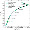 |
Fig. 1. HRD with MS evolutionary tracks for the 16.9 M⊙ 3D MHD merger product (black dashed line) and the 17.4 M⊙ genuine single star (green solid line). The grey and lime-coloured horizontal markers indicate different evolutionary stages, using the central hydrogen mass fraction Xc as a proxy for the evolutionary age, for the merger product and genuine single star, respectively. |
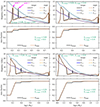 |
Fig. 2. Evolution of the propagation diagrams (odd rows) and hydrogen mass fraction X profiles (even rows) for the 16.9 M⊙ 3D MHD merger product (solid lines) and the 17.4 M⊙ genuine single star (dashed lines). Each panel is labelled with the corresponding central hydrogen mass fractions of the merger product and the genuine single star. |
From the horizontal bar markers on the HRD tracks in Fig. 1, we see that for the same effective temperature Teff and luminosity L★, the two stars are at different MS ages, that is, they have different central hydrogen mass fractions Xc. Initially, the genuine single star still has more hydrogen in its convective core than the merger product when they are in the same position in the HRD. With increasing time, this difference in Xc becomes smaller, reaching a minimum around the time when both stars have Xc≈0.20. At later times, the merger product has a higher value for Xc than the genuine single star for the same Teff and L★.
Although it is instructive to compare the asteroseismic predictions for our models at certain values of Xc (as done, for example, in Wagg et al. 2024), we opted to compare models when they have similar luminosities and effective temperatures. We make this choice because we want to identify distinguishing features in the asteroseismic predictions for a merger product and genuine single star with similar surface diagnostics, which we get from observations. Therefore, in practice, we compare the models at specific Xc values for the merger product. At each of these points in the HRD, we compare the predictions for the merger product with those for the genuine single-star model closest in terms of L★ and Teff. In other words, we compare the models at the positions in the HRD marked by the grey horizontal markers in Fig. 1. The corresponding genuine single-star models have only slightly different values of Xc (at most 2.3%), which can be seen by comparing the top and bottom x-axes in Figs. 3 and B.1a (online appendix).
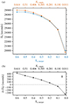 |
Fig. 3. Comparison between the buoyancy travel time Π0 of the 16.9 M⊙ 3D MHD merger product (blue line) and the 17.4 M⊙ genuine single star (red line) as a function of their respective central hydrogen mass fractions Xc (panel a). Panel b shows the absolute differences in Π0, Δ(Π0)=Π0, single−Π0, merger. The error bar in panel b shows σΔP. |
4.1. Asteroseismic comparison
The 16.9 M⊙ 3D MHD merger product and the 17.4 M⊙ genuine single star find themselves in the region of the HRD associated with β Cephei (β Cep) pulsators (Aerts et al. 2010; Aerts 2021). Stars in this class pulsate in numerous low-order p and g modes (e.g. Burssens et al. 2023; Fritzewski et al. 2024), as well as in some high-order g modes (e.g. Daszyńska-Daszkiewicz et al. 2017) when observed in modern space photometry. In this section, we compare the predictions for the g and p modes in this merger product and genuine single star, with and without rotation.
4.1.1. Gravity modes
We start by looking at the difference between the buoyancy travel times Π0 (Eq. 6) for the two objects at different points along their evolution, shown in Fig. 3. We note that we integrate over all regions of the star where  when computing Π0. In other words, we integrate over both the main g-mode cavity and the sub-surface g-mode cavity caused by the iron opacity bump. Serebriakova et al. (2024) find that g modes are able to tunnel through the sub-surface convection zone separating these two mode cavities in stars with masses between 12 and 30 M⊙. Hence, integrating over both mode cavities is appropriate. The buoyancy travel times span a range of roughly 20×103 s to 30×103 s (5.56−8.33 h). The absolute differences between the buoyancy travel times of the merger product and genuine single star (Fig. 3b) have a median value of 173 s and lie in the interval [−349; 426] s. If we convert this to the asymptotic period spacing via Eq. (5), we find that the median values of the difference in Πℓ are 122 s and 71 s for ℓ=1 and ℓ=2, respectively. These values are considerably higher than the currently best uncertainties for observed period spacing values of B-type stars σΔP=50 s (Degroote et al. 2010; Moravveji et al. 2015; Pedersen et al. 2021). At earlier evolutionary stages (higher values of Xc), the genuine single star has a longer buoyancy travel time than the merger product. Around Xc, merger≈Xc, single≈0.15, the merger product overtakes the genuine single star in Π0. In summary, we see that the Π0 values differ for the merger product and genuine single star during large parts of their MS lifetimes, and this difference follows a trend with Xc.
To explain these differences in Π0 for these two types of stars, we compare their g-mode cavities shown in the propagation diagrams in Fig. 2. We identify multiple differences. First, there is the location of the inner boundary of the mode cavity ri, which is equal to the convective core radius Rcc. Since we integrate  to compute Π0, the latter's value is the most sensitive to that of
  at this inner boundary. From Fig. B.1a (online appendix), we see that the absolute difference between Rcc, merger and Rcc, single is at most 0.0125 R⊙ and it follows a similar trend as Δ(Π0) in Fig. 3b. This follows from the fact that a larger convective core leads to a less extended (in radius) g-mode cavity. Second, the leftmost BV frequency peak (‘peak 1’ in the top left panel of Fig. 2), caused by the chemical gradient left behind by the receding convective core, are wider for the genuine single star at all points along the MS. If this were the only difference between the two g-mode cavities, we would expect lower Π0 values of the genuine single star than for the merger product. Third, to the right of this BV frequency peak (peak 1), we see that the genuine single star's
  is lower across multiple solar radii, and the merger product has an additional peak (‘peak 2’) in its
  -profile. This peak results from the transient convective core of the merger product during its thermal relaxation phase described in Sect. 3.2.1. The effect of
  in this region is to lower Π0 for the merger product compared to the one for the genuine single star. Considering all three effects together, we see that the differences in the merger product's and genuine single star's respective Π0 follow the same trend as the convective core radius, but that the point at which the merger product's Π0 becomes larger than the one of the single star occurs later in the evolution than for the convective core radius because of differences in
  in the near-core and envelope regions of both models.
We now turn our attention to the PSPs for ℓ=1 modes (those for ℓ=2 modes are shown in Fig. C.1 in the online appendix in the absence of rotation. Figure 4 shows PSPs constructed using GYRE predictions (see Sect. 3.3) for the 16.9 M⊙ 3D MHD merger product and the 17.4 M⊙ single star at different points along their MS evolution. As expected from the asymptotic period spacing Πℓ, the mean values of the PSPs for the two models are relatively similar. At Xc, single=0.61, we see a quasi-periodic departure of the PSP from its asymptotic behaviour (ΔPn = constant). This quasi-periodic variation is caused by the steep chemical gradient left behind by the receding convective core. This chemical gradient is deduced from the H profiles shown in Fig. 2 and causes a sharp variation in the BV frequency  . We label this sharp variation in
  as ‘peak 1’ in the upper-left panel of Fig. 2. The width of this peak increases with decreasing Xc because of the receding convective core and the subsequent extension of the near-core region with a strong chemical composition gradient. The abrupt change in
  , as seen from the peak, can trap g modes in the peak region, and it is this mode trapping that is responsible for the quasi-periodic deviations from the asymptotic PSP behaviour as observed in MS g-mode pulsators (e.g. Michielsen et al. 2021). Generally, the more the convective core recedes, the higher and broader the
  profile (see Aerts et al. 2021) and the higher the probability of mode trapping. This is apparent from the PSPs for our models shown in Fig. 4. From both theory (Miglio et al. 2008; Cunha et al. 2015, 2019, 2024) and observations (Moravveji et al. 2015, 2016; Michielsen et al. 2021, 2023), we know that the occurrence rate of dips in the PSP is related to the location and width of the sharp variation in
  within the g-mode cavity. Because of the similar location of the sharp
  -variations (peak 1) with respect to the g-mode cavity in the merger product and the genuine single star, the periodicity in the PSP variations is relatively similar. However, there appears to be an additional component to this variation, most clearly seen at Xc, merger=0.60, in the PSPs of the merger product. We attribute this to the presence of a second sharp variation in the
  profile of the merger product, labelled as ‘peak 2’ in the upper-left panel of Fig. 2. This peak is a remnant of the transient convective core described in Sect. 3.2.1, which has left behind a strong chemical gradient at the location of its largest extent. Narrow peaks such as this can perturb and even trap g modes as long as their radial extent is smaller than or comparable to the local wavelength of the modes in question (Cunha 2020). In these cases, the modes experience an abrupt change in
  (as opposed to a smoothly varying
  ), which causes them to be perturbed. We can verify whether this is the case in our model: for modes with a period around 10 days (these are the shortest-wavelength modes considered here), the local wavelengths are λlocal≈0.03 R⊙ and λlocal≈0.15 R⊙ at Xc, merger=0.60 and Xc, merger=0.01, respectively. The full-width-half-maxima (FWHM), which we use as a proxy for the radial extent of the Gaussian-like shape of the second peak, are FWHMpeak 2≈0.02 R⊙ and FWHMpeak 2≈0.08 R⊙ for Xc, merger=0.60 and Xc, merger=0.01, respectively. This shows that we expect this extra peak in the BV frequency profiles of the merger product to affect the g modes since λlocal≳FWHMpeak 2.
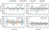 |
Fig. 4. Period spacing patterns for ℓ=1 g modes without rotation for the 16.9 M⊙ 3D MHD merger product (blue solid lines, dot markers) and the 17.4 M⊙ genuine single star (orange solid lines, cross markers) at different evolutionary stages. The horizontal solid black and dashed grey lines indicate the values of the asymptotic period spacing values Πℓ=1 for the merger product and genuine single star, respectively. The |

The amplitude of the PSP variation, that is, the departure of ΔPn from the asymptotic value Πℓ, depends on the sharpness, height, and width of the variation in  (Miglio et al. 2008; Cunha et al. 2015, 2019, 2024). The
  profiles of 26 Slowly Pulsating B-type (SPB) pulsators observed by Kepler and modelled by Pedersen et al. (2021) show a large variety in their sharpness, height, and width. Here, we see that the PSP variations’ amplitudes are similar for the two models, albeit slightly higher for the merger product. The near-core peaks (peak 1) in the BV frequency profiles of the genuine single star are sharper than those for the merger product, while the extra peak in the BV frequency profile of the merger product introduces additional quasi-periodic variability with a different occurrence rate. Despite the similar magnitude of the amplitudes, their differences are typically larger than the observational uncertainties on ΔPn of the B-type stars with the best asteroseismic measurements described by the uncertainty σΔP.
We now repeat the comparison above in the presence of rotation. As argued in Sects. 3.1 and 3.3, we include the effects of rotation (more specifically, the Coriolis force) at the level of the pulsation equations. Figure 5 shows the PSPs for prograde (m>0) and retrograde (m<0) sectoral (ℓ=|m|) g modes predicted for the merger product and genuine single star at Xc, merger=0.50 and Xc, single=0.51, respectively. We consider rotation rates of Ω/Ωc=0.10−0.60, with
 (8)
(8)
the Roche critical angular rotation frequency (Maeder 2009), G the gravitational constant, and Req the stellar radius at the equator of a rotationally deformed star. As expected from Bouabid et al. (2013), the period spacings ΔPn between the prograde modes become smaller with longer oscillation periods and with higher rotation rates, resulting in a negative slope of the PSP, while the retrograde PSPs have positive slopes, in agreement with observations of SPB pulsators (Pápics et al. 2014, 2015, 2017; Szewczuk & Daszyńska-Daszkiewicz 2018; Szewczuk et al. 2021; Pedersen et al. 2021). Overall, we see that the PSPs of the merger product and genuine single star have similar morphologies, that is, they follow the same trends. For prograde modes, the largest differences between the PSPs of the two models are found at shorter periods, but the difference remains clear at longer periods. The main differences in PSP variability are caused by the slightly different positions of the BV peaks. Whereas the average value ΔPn for the merger product is lower than that for the genuine single star at Xc, merger=0.50, the opposite is true for prograde modes with longer periods when we take into account the effects of rotation. This is true for all rotation rates considered here. This can be seen in Fig. 6, where we show the estimated differences the larger-period end2 of the prograde-mode PSPs. We use a fit through the PSPs to make these estimations because it is not possible to do a one-to-one comparison between the modes of these models. Since we computed these PSPs under the TAR with GYRE, it would seem straightforward to fit them with the asymptotic period spacing relation under the TAR (see e.g. Eq. 4 in Bouabid et al. 2013). However, such fits do not return satisfying fitting results when the PSPs deviate strongly from the otherwise smooth asymptotic behaviour under the TAR (Van Reeth et al. 2016), as is the case in our PSPs. Hence, we fitted the PSPs in Fig. 5 with quadratic functions instead. Comparing the estimated differences with σΔP, we see that the differences ΔPn could technically be observed for most prograde dipole (ℓ=1) modes and some prograde quadrupole (ℓ=2) modes in stars with Ω/Ωc≤0.20.
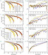 |
Fig. 5. Period spacing patterns (PSPs) for (ℓ, m)=(1, ±1) and (ℓ, m)=(2, ±2) g modes with rotation rates of Ω/Ωc=0.10−0.30 (panels a–d) and Ω/Ωc=0.40−0.60 (panels e–h) for the 16.9 M⊙ 3D MHD merger product and the 17.4 M⊙ genuine single star at Xc, merger=0.50 and Xc, single=0.51, respectively. The black, blue, and grey lines with dot markers correspond to the merger product's PSPs, while the red, orange, and gold lines with cross markers correspond to the PSPs of the genuine single star. The PSPs are shown in the inertial (observer's) frame. |
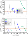 |
Fig. 6. Differences between the quadratic function fits of the PSPs for prograde modes shown in Fig. 5 for Ω/Ωc=0.10−0.30 (top) and Ω/Ωc=0.40−0.60 (bottom). The solid and dashed lines show the differences for the (ℓ, m)=(1, 1) and (ℓ, m)=(2, 2) modes, respectively. The horizontal red line shows the average value of σΔP from observations of SPB pulsators. |
The PSPs for retrograde modes become ‘stretched’ towards longer periods, accentuating the differences in PSP variability between the merger product and genuine single star even more. Lastly, we note the presence of relatively deep dips in the period spacing patterns of both the merger product and genuine single star for different mode morphologies and rotation rates. We do not find such deep dips in the non-rotating case for ℓ=1 modes in the period range shown in Fig. 4, but they are present at longer periods (higher radial order ng) and in the ℓ=2 modes (see Fig. C.1 in the online appendix). Closer inspection shows that these deep dips are caused by the coupling between g modes in the main inner g-mode cavity and those in the subsurface g-mode cavity. This is reminiscent of the g-g-mode coupling described in Unno et al. (1989) and Henneco et al. (2024a).
4.1.2. Low-order pressure modes
Figure 7 shows the frequencies of the low-radial order ℓ=1 and ℓ=2 p modes with radial orders np≤4 and without rotation. Pressure modes with higher radial orders are not observed in β Cep stars (Fritzewski et al. 2024). We compare the predicted p modes for the 16.9 M⊙ 3D MHD merger product and the 17.4 M⊙ genuine single star at different stages during their MS evolution. We find no pure p modes, that is, modes with ng=0 for the models at Xc, merger=0.01 and Xc, merger=0.10 because the structures of the g- and p-mode cavities start to overlap more in frequency, leading to mode mixing (Unno et al. 1989), hence, we leave these evolutionary stages out. Because of their similar p-mode cavities, the p modes in the merger product and genuine single star span a similar frequency range. It is also clear from Figs. 7 and 8 that the p-mode frequencies of the genuine single star are higher by at most 0.3 cycles per day (3.5 μHz). Furthermore, this frequency difference increases with radial order np and decreases with MS age (Fig. 8). Even the smallest frequency difference, which we predict for the fundamental (np=0) ℓ=1 mode at Xc=0.30, has a relative value of ∼10%. This is 1000 times larger than the observed relative p-mode frequency uncertainty of ∼0.01% reported in Aerts et al. (2019) and the absolute p-mode frequency uncertainty of  μHz found for the prototypical β Cep star HD 129929 by Aerts et al. (2003, 2004). Overall, the merger product's p modes are more closely spaced than the genuine single star's.
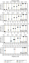 |
Fig. 7. Frequencies and radial orders np of ℓ=1 and ℓ=2 p modes with np≤4 for the 16.9 M⊙ 3D MHD merger product (blue and light-blue markers) and the 17.4 M⊙ genuine single star (red and orange markers) at different evolutionary stages, in the absence of rotation. The models at Xc=0.01 and Xc=0.10 are absent because of the lack of pure p modes at these evolutionary stages. The dot and cross markers show the value of the radial order np for the ℓ=1 and ℓ=2 modes, respectively. The dotted and dash-dotted lines are drawn to accentuate the frequency differences and improve the legibility of the frequency values. |
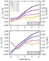 |
Fig. 8. Absolute differences between the 17.4 M⊙ genuine single star's p-mode frequencies |


The difference in p-mode frequencies can be explained by the merger product's lower mean density in its envelope, shown in Fig. B.1b (online appendix). This relates back to the generic principle that since the merger product has the same luminosity, effective temperature, and radius as a more massive genuine single star, its mean envelope molecular weight should be higher and its mean density should be lower, as is indeed the case. The decrease of the difference in p-mode frequencies between the two models with MS age can be attributed to the fact that the merger product's and genuine single star's mean envelope density become similar. Since p modes with higher radial order have more nodes in the region of the star when the merger product and genuine single star differ significantly, they are more sensitive to these differences than those with fewer radial nodes. Just as for g modes, we see that the differences between the merger product's and genuine single star's predicted asteroseismic characteristics are largest when the stars are younger.
Analogue to the g modes, we consider the effect of rotation, more specifically the Coriolis force. We treat it perturbatively up to first order in the rotation frequency, which is a good approximation for the p modes for slow and modest rotators. Its influence on the p modes and on the frequency difference found in the absence of rotation can be found in the online appendix. We find that, at least with perturbative implementation of the effect of the Coriolis force, the differences in p-mode frequencies between the merger product and genuine single star are similar to those in the absence of rotation.
4.2. Comparison with and between 1D merger methods
We now investigate if and how the predictions made in Sect. 4.1 differ when we use 1D merger prescriptions. As mentioned in Sect. 1, we consider three commonly used 1D merger prescriptions: entropy sorting, entropic variable sorting with shock heating (PyMMAMS), and fast accretion (see Sect. 3.2). The HRD in Fig. 9 shows evolutionary tracks of the merger products acquired with all four methods (the 3D MHD simulation and the three 1D methods). We see that the tracks do not coincide in the HRD, which results in each merger product approximately overlapping with a genuine single star of a different mass. As detailed at the beginning of Sect. 4, the track for the entropy-sorted model comes closest to that of the 3D MHD model; its corresponding genuine single star has a mass of 17.15 M⊙. Using the entropy sorting method, we under-predict Π0 by at most 450 s in comparison to the 3D MHD model. The error one would make by using entropy sorting instead of the 3D MHD model would thus be around 9×σΔP. In other words, the error we make by using entropy sorting is of the same order as the difference in Π0 between the 3D MHD merger product model and its corresponding genuine single star (see Sect. 4.1.1). With entropy sorting, we under-predict this Π0 difference between the merger product and its corresponding genuine single star compared to the 3D MHD merger product (Fig. 10b). This difference has a median value of 213 s and lies in the interval [−36; 402] s.
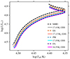 |
Fig. 9. HRD with the evolutionary tracks of the 16.9 M⊙ merger product computed with the 3D MHD simulation (MHD, black dashed line), entropy sorting (ES, red dashed line), PyMMAMS (PM, blue dashed line), and fast accretion (FA, indigo dashed line). The corresponding 17.4 M⊙, 17.15 M⊙, 17.0 M⊙, and 16.9 M⊙ genuine single stars evolutionary tracks are drawn with grey, orange, cyan, and magenta solid lines, respectively. |
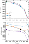 |
Fig. 10. Comparison between the buoyancy travel time Π0 for the 16.9 M⊙ 3D MHD (MHD, black line), entropy-sorted (ES, red line), PyMMAMS (PM, blue line), and fast accretion (FA, indigo line) merger products (panel a), and the absolute differences Δ(Π0)=Π0, single−Π0, merger with their respective genuine single star models (panel b). The error bar in panel b shows the σΔP. |
The HRD tracks of the PyMMAMS and fast accretion merger products also lie below that of the 3D merger product, corresponding to genuine single-star models with masses of 17.0 M⊙ and 16.9 M⊙, respectively (Fig. 9). With both methods, we under-predict Π0 compared to the 3D MHD merger product by at least 657 s and 257 s, and at most 850 s and 590 s for the PyMMAMS and fast-accretion merger product, respectively. The resulting differences in Πℓ are significantly larger than σΔP. With the PyMMAMS method, we over-predict the difference in Π0 compared to its corresponding genuine single star. The median value of this difference is 420 s and it lies in the interval [246; 583] s. With the fast accretion method, we under-predict the difference in Π0 between the merger product and the genuine single star. This absolute difference has a median value of −87 s and lies in the interval [−726; 61] s. The Π0 difference between all merger products and their genuine single-star counterparts increases abruptly in absolute value at Xc, merger=0.01. We attribute this to the fact that there is a noticeable difference between the HRD tracks around the Henyey hook (the point where logTeff starts increasing; see Fig. 9). The overall differences in the Π0 values and differences in Π0 between the merger products obtained through 1D methods and their corresponding genuine single stars can be explained by the differences in the merger products’ BV profiles compared to the 3D MHD merger product. We highlight these differences in the following sections.
4.2.1. Entropy-sorted merger product
From Fig. E.1 in the online appendix, we see that the near-core region of the entropy-sorted merger product model is enriched in He, but less strongly and over a smaller radial extent than what we found in the model for the 3D MHD merger product. Contrary to the 3D MHD merger product, the entropy-sorting method does not lead to the He-rich core of the primary star ending up in a shell around the secondary's core. The He enrichment originates from the secondary's core – also enriched in He, though less strongly than the primary's – which forms a layer around the merger product's core. Additionally, transient convective zones emerge around the core-envelope boundary during the thermal relaxation phase, mixing He-rich core material into the near-core region. Contrary to the 3D MHD model, the entropy sorted model does not have a transient convective core before starting its MS evolution. However, its BV frequency profile contains multiple Gaussian-like peaks (Fig. E.1 in the online appendix) due to the staircase-like structure of the chemical composition profile, which has two origins. The first origin is the entropy-sorting method itself, which can result in large jumps in the chemical composition between neighbouring layers of the star. The second origin is the appearance of short-lived, numerically unstable convection zones before the merger product settles on the MS.
Looking at the predicted PSPs for the entropy-sorted merger model and its 17.15 M⊙ genuine single-star counterpart in Fig. 11, we see a similar trend in the asymptotic period spacings Πℓ as in the case of the 3D MHD merger product. The values of Πℓ for the merger product and genuine single star differ by more than σΔP, yet these differences are, in general, somewhat higher (except at Xc, merger=0.60) than what we predict for the 3D MHD merger product. The variability in the PSPs of the entropy-sorted model is seemingly more chaotic than that for the 3D MHD merger product because the modes are affected by multiple peaks in the  -profile. The amplitude of the variability is also higher for the entropy-sorted model.
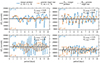 |
Fig. 11. Same as Fig. 4 but for the 16.9 M⊙ entropy sorted merger product (blue solid lines, dot markers) and the 17.15 M⊙ genuine single star (orange solid lines, cross markers). |
From Figs. 12 and 13, we see that the predicted p modes for the entropy-sorted merger product model behave qualitatively similarly to those predicted for the 3D MHD model. However, we under-predict the differences in ℓ=1 and ℓ=2 p-mode frequencies between the merger product and genuine single star by up to 0.14 cycles/day (1.62 μHz) compared to the 3D MHD model, which is more than two orders of magnitude larger than  μHz (Aerts et al. 2003, 2004). Furthermore, the frequency error we make by using entropy sorting instead of the 3D MHD model, shown in the bottom panel of Fig. 8, is of the order of 0.03−0.05 cycles/day (0.35−0.58 μHz) and is also significantly larger than
  . We attribute these frequency shifts to the different chemical structures (Fig. E.1 in the online appendix) the two merger product models have in their p-mode cavities (see Sect. 4.1.2).
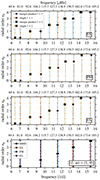 |
Fig. 12. Mode frequencies and radial orders np for (ℓ, m)=(1, 0) and (ℓ, m)=(2, 0) p modes in the absence of rotation at Xc, merger=0.50 for the entropy-sorted (ES), PyMMAMS (PM), and fast accretion (FA) merger product models and their corresponding genuine single-star models. In the top three panels, the colour, line, and marker conventions are the same as in Fig. 7. The bottom panel shows the (ℓ, m)=(1, 0) p mode frequencies for the 3D MHD, entropy-sorted, PyMMAMS, and fast accretion models together. |
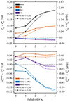 |
Fig. 13. Absolute differences between the 17.4 M⊙, 17.15 M⊙, 17.0 M⊙, and 16.9 M⊙ genuine single star's p mode frequency |


4.2.2. PyMMAMS merger product
Thanks to the addition of shock heating in the PyMMAMS prescription, it performs better in reproducing the overall merger product structure expected from the 3D MHD simulation. Contrary to the entropy sorted model, the PyMMAMS prescription results in the secondary's core sinking to the centre of the merger product and the primary's core forming a shell around it (see Fig. E.2 in the online appendix). However, we find that by comparing the chemical composition profiles for the 3D MHD andPyMMAMS merger products (Figs. 2 and E.2), the He-enrichment of the merger product's envelope is limited to the near-core region (up to r≈1.8 R⊙ at Xc=0.60) in the PyMMAMS model, whereas the enrichment extends further out to r≈3.0 R⊙ in the 3D MHD model. A second difference between the 3D MHD, entropy-sorted, and PyMMAMS models is the lack of an extended transient convective core during the merger product's thermal relaxation phase before settling back on the MS in the latter model. The extra peak in the  profile (peak 2), present in the 3D MHD, is missing in the PyMMAMS model. As a result, the BV frequency profiles for this merger product and its corresponding 17.0 M⊙ genuine single star model look almost identical (Fig. E.2 in the online appendix). Only the radial extent of the BV frequency peak of the merger product is larger than in the genuine single-star model because of the He-enrichment in the near-core region. The lack of an additional peak in the BV frequency profile of the PyMMAMS model causes there to be no additional variability in the merger model's PSPs (Fig. A.1a). The two PSPs have roughly the same quasi-periodic behaviour, albeit with a relatively small phase shift likely caused by the more extended BV frequency peak of the PyMMAMS merger product. However, the phase shift and difference in ΔPn are still larger than the currently best uncertainty of g-mode periods
  days (Moravveji et al. 2015) and σΔP, respectively.
Because of the virtually identical chemical composition profiles and p-mode cavities (Fig. E.2 in the online appendix), we find that the p-mode frequency absolute differences between the PyMMAMS merger model and its corresponding genuine single star are negative and ≤0.02 cycles/day (≤0.23 μHz), shown in the top panel of Fig. 8. This is an order of magnitude larger than  . The p-mode frequency error compared to the 3D MHD model (bottom panel of Fig. 8) is of the order of 0.1 cycles/day (1.16 μHz), several orders of magnitude larger than
  .
.
4.2.3. Fast accretion merger product
Although the fast accretion method has proven to be sufficient in reproducing low-mass (Rui & Fuller 2021) and massive (Henneco et al. 2024a) post-MS merger products, it does not perform well for MS merger products. For massive post-MS merger products, the sub-thermal-timescale accretion onto a blue Hertzsprung-gap star emulating the merger leads to the formation of long-lived blue supergiant stars with distinct structures. In the MS case, we see that the fast accretion phase leads to a transient convective core, yet this core has a smaller extent than what we found in the 3D MHD and entropy-sorted model. This transient convective core and the subsequent receding rejuvenated convective core leave an imprint in the chemical composition profile, which results in double-peaked BV frequency profile in the near-core region (Fig. E.3 in the online appendix), similar to the one found in Wagg et al. (2024). From Henneco et al. (2024a), we expect that the extent of this transient convective core depends on the mass added to the primary star, the accretion timescale, and the semi-convective efficiency (Braun & Langer 1995). We see from Fig. A.1b that the second BV frequency peak influences the PSP variability mostly in the number of modes found in the PSP dips and the amplitude, which are both higher for the merger product.
On the level of the p modes, we see similar behaviour as for the PyMMAMS model. Since we assumed that the composition of the accreted material is that of the surface of the accreting star, the envelope of the merger product is not enriched in helium. Because of the small radial extent of the transient convective core during the merger procedure, the p-mode cavity is virtually identical to the 16.9 M⊙ genuine single star's p-mode cavity. The frequency differences between the merger product and genuine single star are at most 0.025 cycles/day (0.289 μHz). The frequency error compared to the 3D MHD merger product's p modes is in the interval [−0.025; 0.036] cycles/day ([−0.289; 0.417] μHz), but is larger in absolute value than  for all radial orders (bottom panel of Fig. 8).
4.2.4. Potential improvements to 1D merger prescriptions
Since none of the 1D merger prescription models is able to reproduce the interior structure and asteroseismic predictions of the 3D MHD model, we briefly discuss some ways in which these methods could potentially be improved. Neither the mean asymptotic period spacing values nor the PSP variability morphology of the 3D MHD merger product model are reproduced well with the fast accretion method. A potential improvement to this method would be to abandon the assumption that the chemical composition of the accreted material is the same as that of the accretor's surface and instead accrete the full chemical composition of the secondary star. However, this has the drawback that one needs to make assumptions about the mixing of this material in the accretor's envelope.
The PyMMAMS model performed worse than the entropy-sorted model, but has the highest potential for improvement, especially since it predicts the correct overall chemical structure of the merger product (secondary core in the centre, primary core around it). As mentioned in Sect. 3.2.3, the main difference between entropy-sorting and PyMMAMS is the inclusion of shock heating in the latter. Evidently, the shock heating, calibrated on more energetic head-on collisions, does not lead to a satisfactory reproduction of the 3D MHD model. However, provided that more 3D binary merger simulations become available, they could be used to calibrate the shock heating prescription in PyMMAMS to better reproduce the chemical composition profiles resulting from these slower, less energetic binary inspiral mergers (Heller et al., in prep.). In the limit where a calibrated PyMMAMS version reproduces a model with the exact same chemical composition profiles as the 3D MHD model, we expect the subsequent evolution and asteroseismic signals to be the same.
4.3. Discussion
In summary, the structural and chemical anomalies resulting from the merger lead, as shown in Sect. 4.1.1, to different asymptotic period spacings Πℓ and hence mean PSP values for the merger product and genuine single star. The differences in the asymptotic period spacing are of the order of several 10 s to 100 s, which is larger than the current best uncertainties on g-mode period spacing patterns of σΔP≃50 s. However, as we have shown, this difference in the asymptotic period spacing changes as the star evolves (Fig. 3). Also, for prograde sectoral modes computed under the TAR, the differences in PSP values are smaller than without rotation, and the PSP values are, on average, higher for the merger product than for the genuine single star, whereas the opposite is true in the non-rotating case (at Xc=0.50). In other words, if observed period spacing patterns are available, their mean value likely does not unambiguously allow us to distinguish this type of merger product from genuine single stars.
We can look at this from another angle. In Fig. 14, we show the asymptotic period spacing for ℓ=1 modes Πℓ=1=Π1 for the 3D MHD merger product at Xc=0.50 and genuine single stars in a typical observational box centred around the HRD location of the merger product with a size of log(L★/L⊙)±0.1 dex and Teff±1000 K. As readily seen in Sect. 4.1.1, the difference in Π1 is several times higher than σΔP=50 s for the merger product and its closest genuine single star model. Going to higher and lower masses, the absolute value of the difference in Π1 quickly grows. In the limit of infinitely accurate measurements of L★ and Teff, we do expect the merger product to be an outlier in terms of Π1. However, at slightly lower logTeff and similar logL★ – within the typical uncertainties on L★ and Teff mentioned above – we find genuine single-star models with Π1 values comparable to that of the merger product. Thus, we would need highly accurate measurements of L★ and Teff to distinguish this particular merger product; of the order of 0.001 dex in logTeff. In other words, given today's typical uncertainties on L★ and Teff, we predict that the merger product is likely indistinguishable from genuine single stars based on its Π1 value.
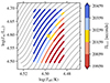 |
Fig. 14. Values of Πℓ=1=Π1 for the 3D MHD merger product at Xc=0.50 (cross marker, |
As described in Sect. 4.1.2, frequencies of p modes are lower and more closely spaced in the merger product compared to the genuine single star, which we attribute to the merger product's lower mean density and sound speed in its p-mode cavity. These mean values converge with MS age, making the differences in p-mode frequencies smaller. Nevertheless, the differences are still larger than the current best relative uncertainties on observed p-mode frequencies of 0.01% (Aerts et al. 2019, Table 1). Additionally, the differences increase with increasing radial order because of the higher sensitivity of these modes to the chemical composition in the p-mode cavity. We also found that the frequency differences between the merger product and genuine single star are virtually insensitive to the rotation rate as a consequence of the first-order Ledoux perturbative approach used to include rotation on the level of the pulsation equations only. Especially at higher rotation rates, the effects of the centrifugal deformation of the star on p modes should not be ignored (see Aerts & Tkachenko 2024 for an overview). Overall, our analysis shows that the differences in p-mode frequencies are of the order of 0.10 cycles/day (1.16 μHz) and depend strongly on the chemical composition of the p-mode cavity, which is the part of the star where the merger product deviates the most from its corresponding genuine single star.
We emphasise that a merger between two stars will leave a chemical signature in the merger product's envelope (Glebbeek et al. 2013). Exceptions are unevolved stars close to the zero-age main sequence (ZAMS), symmetrical binaries (i.e. nearly equal mass stars that have evolved quasi-identical before the merger. This assumes that no significant mass transfer occurs during the contact phase of such systems), or mergers in which both progenitor cores end up in the product's core (with no chemical enrichment of the envelope of the result). This signature does depend on, for example, the mixing processes during and after the merger and will influence the asteroseismic signatures.
In our assessment of the performance of the three 1D merger methods, we find that none of the 1D methods can replicate the 3D MHD model structure. Entropy sorting performs best for this particular merger product even though this is likely coincidental. This method fails to reproduce the behaviour found in the 3D merger product model where the He-rich core of the primary star forms a layer around the secondary star's core, leading to strong and radially extended He-enrichment in the lower envelope. The PyMMAMS prescription does lead to an overall correct chemical structure for the merger product, yet, the radial extent of the He-enrichment of the envelope is less than in the 3D MHD model. By design, the fast accretion method is unable to reproduce the overall structure of the 3D MHD model, which is unlikely to improve by accreting material with a more realistic composition (see Sect. 4.2.4). Because of the sensitivity of both g and p modes to the interior chemical structure, the asteroseismic predictions differ depending on which 1D merger prescription we used. More importantly, none of the asteroseismic predictions based on 1D merger prescription equilibrium models managed to reproduce those for the 3D MHD model within the observational uncertainties. In other words, all 1D methods introduce errors in the predicted ΔPn and νp that are larger than the current best observational uncertainties. Moreover, even with the best-performing method, entropy sorting, the error we make in Π0 is of the same order as the predicted Π0 differences between the 3D MHD merger model and its corresponding genuine single star. Therefore, it would be quite problematic if one were to use these 1D merger methods to create merger models for asteroseismic fitting and forward modelling purposes. Overall, as explained in Sect. 4.2.4, the PyMMAMS model has the most potential to produce merger product models consistent with those obtained from 3D simulations on the condition that it is calibrated for binary mergers.
5. Conclusions
We find from the results presented in Sect. 4 that even though the resulting product of a stellar merger between a 9 M⊙ and a 8 M⊙ MS star leads a seemingly ‘normal’ MS life, its structure and composition are rather anomalous compared to genuine single stars. The 16.9 M⊙ merger product obtained from the 3D MHD simulation of Schneider et al. (2019) has an abnormally high convective core radius and stellar radius for its respective mass. More specifically, throughout its MS evolution, the merger product's convective core and stellar radii are similar to those of a more massive 17.4 M⊙ genuine single star with similar effective temperature and luminosity. Given that the merger product overlaps in the HRD with a more massive star, its L★/M★ is higher than that of genuine single stars. We have shown in Sect. 4 that this can be explained by the He-enrichment of the envelope of the merger product and should be a generic feature in stars with chemically enriched envelopes.
The quasi-periodic variation found in the PSPs has the additional potential of singling out merger products from photometric light curves. The merger product's PSP variability contains approximately the same component as the genuine single star's, namely that caused by the strong BV frequency peak in their near-core regions. However, the extra peak in the merger product's BV frequency profile introduces a second component to this variability. Although it is harder to see at later MS stages, this second component in the merger product's variability distorts the somewhat regular behaviour of the variability that we would expect without the effect of the additional peak. This becomes clear when comparing the PSPs of the merger product and the genuine single star. A promising diagnostic for the presence of a merger product would be to look for such irregularities in observed PSPs. For that, mode identification (assigning n, ℓ, and m values to individual modes) is required, which currently lies within the realm from combined Gaia and TESS space photometry (Hey & Aerts 2024; Fritzewski et al. 2024). One could then look for and characterise components in the PSP variability, such as those predicted in this work. After this characterisation, tools such as those developed by Miglio et al. (2008) and Cunha et al. (2024, and references therein) could be used to link potential merger products’ particular PSP variability to their internal structure. These tools are derived for non-rotating stars. So, before they can be used, the effect of the Coriolis force, which dominates the PSPs’ deviation from their asymptotic consonant behaviour (i.e. the slopes of the PSPs), needs to be modelled first using TAR-based PSP predictions. Various generalisations to the basic PSP predictions based on the TAR have been published, including the effects of differential rotation (Van Reeth et al. 2018), small centrifugal deformation (Henneco et al. 2021; Dhouib et al. 2021), and an additional internal magnetic field (Dhouib et al. 2022). However, none of these theoretical predictions have been applied in practical applications to single stars, and their quality remains to be evaluated.
We have shown that the differences between the mean ΔPn and/or p-mode frequencies νp of a merger and genuine single star of similar mass are comfortably above the current best observational uncertainties. However, we have also shown in Fig. 14 that the merger product treated in this work will likely not manifest as an outlier based on its mean period spacing unless one has highly accurate Teff and L★ measurements. Therefore, applications will benefit from additional constraints aside from asteroseismic ones. Surface diagnostics such as abundances and L★/M★ estimates, for example, could help to firmly identify MS merger products. Moreover, fitting observed properties with genuine single-star and merger models and their pulsation predictions may lead to systematic offsets in their derived masses, ages, pulsation frequencies, etc. between the two best solutions. For such forward modelling applications to become possible, extensive grids of merger product models are required in addition to single-star model grids.
It is imperative to keep in mind when interpreting the results presented in this work that we focus on one particular type of MS merger product, formed through the merger of two relatively young MS stars with a mass ratio close to one. The differences presented in this work are, therefore, lower limits on the differences that can be expected for merger products in general. From, for example, the set of merger products described in Glebbeek et al. (2013), we know that depending on the age and binary configuration of a stellar merger's progenitor system, qualitatively different merger products can be achieved that might have different asteroseismic characteristics compared to equivalent genuine single stars. To answer the question of whether we can use asteroseismology to distinguish MS merger products from genuine single stars and to eventually create grids of MS merger models for forward modelling, the analysis presented in this work ought to be repeated on a range of different MS merger products. Doing this requires a cohesive set of 3D merger simulations, similar to those of Glebbeek et al. (2013), but for mergers driven by binary evolution. As demonstrated in this work, we should be wary of resorting to 1D merger prescriptions unless they are calibrated on the results of 3D simulations. Additionally, more realistic predictions for the asteroseismic fingerprints of stellar merger products also require us to take large-scale magnetic fields into account in our evolution models and asteroseismic predictions, given that they are predicted (Schneider et al. 2019; Ryu et al. 2025) and inferred from observations (Schneider et al. 2020; Frost et al. 2024) to be present in these stars.
Data availability
The online appendix containing supplementary figures, as well as the in- and output files for this work, are available at https://doi.org/10.5281/zenodo.15194414
Acknowledgments
We wish to thank the referee, Nicholas Rui, for his valuable comments and suggestions, which have helped us further improve this work. We thank T. Neumann for the valuable insights from her Bachelor thesis titled ‘Probing merger methods in a 9 M⊙ and 8 M⊙ binary star system’ (University of Heidelberg, 2022). We thank L. Buchele, T. Van Reeth, Q. Coppée, and D. Bowman (in no particular order) for the meaningful discussions and valuable comments and suggestions. Additional software used in this work includes PyGYRE (Townsend & Rosenberg 2020), PyMesaReader (Wolf & Schwab 2017), MPI for Python (Dalcín et al. 2005; Dalcin & Fang 2021), Astropy (Astropy Collaboration 2013, 2018, 2022), NumPy (Harris et al. 2020), and SciPy (Virtanen et al. 2020). We used Matplotlib (Hunter 2007) for plotting. The authors acknowledge support from the Klaus Tschira Foundation. This work has received funding from the European Research Council (ERC) under the European Union's Horizon 2020 research and innovation programme (Starting Grant agreement N° 945806: TEL-STARS, Consolidator Grant agreement N° 101000296: DipolarSound, and Synergy Grant agreement N°101071505: 4D-STAR). While funded by the European Union, views and opinions expressed are however those of the author(s) only and do not necessarily reflect those of the European Union or the European Research Council. Neither the European Union nor the granting authority can be held responsible for them. This work is supported by the Deutsche Forschungsgemeinschaft (DFG, German Research Foundation) under Germany's Excellence Strategy EXC 2181/1-390900948 (the Heidelberg STRUCTURES Excellence Cluster).
We use a tilde to emphasise that we use the linear definitions of the Lamb and BV frequencies instead of their often used angular forms. They are related to each other as  and
and  .
.
We only consider modes with periods Pn satisfying  , with
  and
and  the minimum and maximum period shown in Fig. 5.
References
- Aerts, C. 2021, Rev. Mod. Phys., 93, 015001 [Google Scholar]
- Aerts, C., & Tkachenko, A. 2024, A&A, 692, R1 [NASA ADS] [CrossRef] [EDP Sciences] [Google Scholar]
- Aerts, C., Thoul, A., Daszyńska, J., et al. 2003, Science, 300, 1926 [Google Scholar]
- Aerts, C., Waelkens, C., Daszyńska-Daszkiewicz, J., et al. 2004, A&A, 415, 241 [NASA ADS] [CrossRef] [EDP Sciences] [Google Scholar]
- Aerts, C., Christensen-Dalsgaard, J., & Kurtz, D. W. 2010, Asteroseismology (Dordrecht: Springer) [Google Scholar]
- Aerts, C., Molenberghs, G., Michielsen, M., et al. 2018, ApJS, 237, 15 [Google Scholar]
- Aerts, C., Mathis, S., & Rogers, T. M. 2019, ARA&A, 57, 35 [Google Scholar]
- Aerts, C., Augustson, K., Mathis, S., et al. 2021, A&A, 656, A121 [NASA ADS] [CrossRef] [EDP Sciences] [Google Scholar]
- Anders, E. H., Lecoanet, D., Cantiello, M., et al. 2023, Nat. Astron., 7, 1228 [NASA ADS] [CrossRef] [Google Scholar]
- Asplund, M., Grevesse, N., Sauval, A. J., & Scott, P. 2009, ARA&A, 47, 481 [NASA ADS] [CrossRef] [Google Scholar]
- Astropy Collaboration (Robitaille, T. P., et al.) 2013, A&A, 558, A33 [NASA ADS] [CrossRef] [EDP Sciences] [Google Scholar]
- Astropy Collaboration (Price-Whelan, A. M., et al.) 2018, AJ, 156, 123 [Google Scholar]
- Astropy Collaboration (Price-Whelan, A. M., et al.) 2022, ApJ, 935, 167 [NASA ADS] [CrossRef] [Google Scholar]
- Auvergne, M., Bodin, P., Boisnard, L., et al. 2009, A&A, 506, 411 [NASA ADS] [CrossRef] [EDP Sciences] [Google Scholar]
- Ballone, A., Costa, G., Mapelli, M., et al. 2023, MNRAS, 519, 5191 [NASA ADS] [CrossRef] [Google Scholar]
- Balona, L. A. 2024, Universe, 10, 437 [Google Scholar]
- Bellinger, E. P., de Mink, S. E., van Rossem, W. E., & Justham, S. 2024, ApJ, 967, L39 [NASA ADS] [CrossRef] [Google Scholar]
- Berthomieu, G., Gonczi, G., Graff, P., Provost, J., & Rocca, A. 1978, A&A, 70, 597 [Google Scholar]
- Bessila, L., & Mathis, S. 2024, A&A, 690, A270 [NASA ADS] [CrossRef] [EDP Sciences] [Google Scholar]
- Bhattacharya, S., Das, S. B., Bugnet, L., Panda, S., & Hanasoge, S. M. 2024, ApJ, 970, 42 [NASA ADS] [CrossRef] [Google Scholar]
- Böhm-Vitense, E. 1958, ZAp, 46, 108 [NASA ADS] [Google Scholar]
- Bouabid, M. P., Dupret, M. A., Salmon, S., et al. 2013, MNRAS, 429, 2500 [Google Scholar]
- Bowman, D. M. 2023, Ap&SS, 368, 107 [NASA ADS] [CrossRef] [Google Scholar]
- Bowman, D. M., Burssens, S., Pedersen, M. G., et al. 2019, Nat. Astron., 3, 760 [Google Scholar]
- Bowman, D. M., Van Daele, P., Michielsen, M., & Van Reeth, T. 2024, A&A, 692, A49 [NASA ADS] [CrossRef] [EDP Sciences] [Google Scholar]
- Braun, H., & Langer, N. 1995, A&A, 297, 483 [NASA ADS] [Google Scholar]
- Britavskiy, N., Lennon, D. J., Patrick, L. R., et al. 2019, A&A, 624, A128 [NASA ADS] [CrossRef] [EDP Sciences] [Google Scholar]
- Burssens, S., Bowman, D. M., Michielsen, M., et al. 2023, Nat. Astron., 7, 913 [NASA ADS] [CrossRef] [Google Scholar]
- Castro, N., Fossati, L., Langer, N., et al. 2014, A&A, 570, L13 [NASA ADS] [CrossRef] [EDP Sciences] [Google Scholar]
- Claeys, J. S. W., de Mink, S. E., Pols, O. R., Eldridge, J. J., & Baes, M. 2011, A&A, 528, A131 [NASA ADS] [CrossRef] [EDP Sciences] [Google Scholar]
- Cox, J. P., & Giuli, R. T. 1968, Principles of Stellar Structure (New York: Gordon and Breach) [Google Scholar]
- Cunha, M. S. 2020, Astrophys. Space Sci. Proc., 57, 185 [Google Scholar]
- Cunha, M. S., Stello, D., Avelino, P. P., Christensen-Dalsgaard, J., & Townsend, R. H. D. 2015, ApJ, 805, 127 [NASA ADS] [CrossRef] [Google Scholar]
- Cunha, M. S., Avelino, P. P., Christensen-Dalsgaard, J., et al. 2019, MNRAS, 490, 909 [Google Scholar]
- Cunha, M. S., Damasceno, Y. C., Amaral, J., et al. 2024, A&A, 687, A100 [NASA ADS] [CrossRef] [EDP Sciences] [Google Scholar]
- Dalcin, L., & Fang, Y. -L. L. 2021, Comput. Sci. Eng., 23, 47 [NASA ADS] [CrossRef] [Google Scholar]
- Dalcín, L., Paz, R., & Storti, M. 2005, J. Parallel Distrib. Comput., 65, 1108 [CrossRef] [Google Scholar]
- Dale, J. E., & Davies, M. B. 2006, MNRAS, 366, 1424 [NASA ADS] [Google Scholar]
- Daszyńska-Daszkiewicz, J., Pamyatnykh, A. A., Walczak, P., et al. 2017, MNRAS, 466, 2284 [CrossRef] [Google Scholar]
- de Mink, S. E., Pols, O. R., & Hilditch, R. W. 2007, A&A, 467, 1181 [NASA ADS] [CrossRef] [EDP Sciences] [Google Scholar]
- Degroote, P., Aerts, C., Baglin, A., et al. 2010, Nature, 464, 259 [Google Scholar]
- Dhouib, H., Prat, V., Van Reeth, T., & Mathis, S. 2021, A&A, 652, A154 [NASA ADS] [CrossRef] [EDP Sciences] [Google Scholar]
- Dhouib, H., Mathis, S., Bugnet, L., Van Reeth, T., & Aerts, C. 2022, A&A, 661, A133 [NASA ADS] [CrossRef] [EDP Sciences] [Google Scholar]
- Eckart, C. 1960, Phys. Fluids, 3, 421 [Google Scholar]
- Ferguson, J. W., Alexander, D. R., Allard, F., et al. 2005, ApJ, 623, 585 [Google Scholar]
- Ferrario, L., Pringle, J. E., Tout, C. A., & Wickramasinghe, D. T. 2009, MNRAS, 400, L71 [NASA ADS] [CrossRef] [Google Scholar]
- Ferraro, F. R., Lanzoni, B., Dalessandro, E., et al. 2012, Nature, 492, 393 [Google Scholar]
- Freitag, M., & Benz, W. 2005, MNRAS, 358, 1133 [Google Scholar]
- Fritzewski, D. J., Vanrespaille, M., Aerts, C., et al. 2024, A&A, in press, https://doi.org/10.1051/0004-6361/202451721 [Google Scholar]
- Frost, A. J., Sana, H., Mahy, L., et al. 2024, Science, 384, 214 [NASA ADS] [CrossRef] [Google Scholar]
- Gaburov, E., Lombardi, J. C., & Portegies Zwart, S. 2008, MNRAS, 383, L5 [NASA ADS] [Google Scholar]
- Garcia, S., Van Reeth, T., De Ridder, J., & Aerts, C. 2022, A&A, 668, A137 [NASA ADS] [CrossRef] [EDP Sciences] [Google Scholar]
- Glebbeek, E., Pols, O. R., & Hurley, J. R. 2008, A&A, 488, 1007 [NASA ADS] [CrossRef] [EDP Sciences] [Google Scholar]
- Glebbeek, E., Gaburov, E., Portegies Zwart, S., & Pols, O. R. 2013, MNRAS, 434, 3497 [NASA ADS] [CrossRef] [Google Scholar]
- Guo, Z. 2021, Front. Astron. Space Sci., 8, 67 [NASA ADS] [Google Scholar]
- Guo, Z., Ogilvie, G. I., Li, G., Townsend, R. H. D., & Sun, M. 2022, MNRAS, 517, 437 [NASA ADS] [CrossRef] [Google Scholar]
- Harris, C. R., Millman, K. J., van der Walt, S. J., et al. 2020, Nature, 585, 357 [NASA ADS] [CrossRef] [Google Scholar]
- Hatt, E. J., Ong, J. M. J., Nielsen, M. B., et al. 2024, MNRAS, 534, 1060 [NASA ADS] [CrossRef] [Google Scholar]
- Hekker, S., & Christensen-Dalsgaard, J. 2017, A&ARv, 25, 1 [Google Scholar]
- Henneco, J., Van Reeth, T., Prat, V., et al. 2021, A&A, 648, A97 [EDP Sciences] [Google Scholar]
- Henneco, J., Schneider, F. R. N., Hekker, S., & Aerts, C. 2024a, A&A, 690, A65 [NASA ADS] [CrossRef] [EDP Sciences] [Google Scholar]
- Henneco, J., Schneider, F. R. N., & Laplace, E. 2024b, A&A, 682, A169 [NASA ADS] [CrossRef] [EDP Sciences] [Google Scholar]
- Hey, D., & Aerts, C. 2024, A&A, 688, A93 [NASA ADS] [CrossRef] [EDP Sciences] [Google Scholar]
- Hunter, J. D. 2007, Comput. Sci. Eng., 9, 90 [NASA ADS] [CrossRef] [Google Scholar]
- Iglesias, C. A., & Rogers, F. J. 1993, ApJ, 412, 752 [Google Scholar]
- Iglesias, C. A., & Rogers, F. J. 1996, ApJ, 464, 943 [NASA ADS] [CrossRef] [Google Scholar]
- Kippenhahn, R., Weigert, A., & Weiss, A. 2013, Stellar Structure and Evolution (Berlin, Heidelberg: Springer) [Google Scholar]
- Koch, D. G., Borucki, W. J., Basri, G., et al. 2010, ApJ, 713, L79 [Google Scholar]
- Kurtz, D. W. 2022, ARA&A, 60, 31 [NASA ADS] [CrossRef] [Google Scholar]
- Laplace, E., Justham, S., Renzo, M., et al. 2021, A&A, 656, A58 [NASA ADS] [CrossRef] [EDP Sciences] [Google Scholar]
- Lee, U., & Saio, H. 1987, MNRAS, 224, 513 [Google Scholar]
- Li, G., Van Reeth, T., Bedding, T. R., et al. 2020, MNRAS, 491, 3586 [Google Scholar]
- Lombardi, J. C., Rasio, F. A., & Shapiro, S. L. 1996, ApJ, 468, 797 [NASA ADS] [CrossRef] [Google Scholar]
- Ma, L., Johnston, C., Bellinger, E. P., & de Mink, S. E. 2024, ApJ, 966, 196 [NASA ADS] [CrossRef] [Google Scholar]
- Maeder, A. 2009, Physics, Formation and Evolution of Rotating Stars (Berlin, Heidelberg: Springer) [Google Scholar]
- Mapelli, M., Sigurdsson, S., Ferraro, F. R., et al. 2006, MNRAS, 373, 361 [Google Scholar]
- Marchant, P., Langer, N., Podsiadlowski, P., Tauris, T. M., & Moriya, T. J. 2016, A&A, 588, A50 [NASA ADS] [CrossRef] [EDP Sciences] [Google Scholar]
- Mathis, S. 2009, A&A, 506, 811 [CrossRef] [EDP Sciences] [Google Scholar]
- Mennekens, N., & Vanbeveren, D. 2017, A&A, 599, A84 [NASA ADS] [CrossRef] [EDP Sciences] [Google Scholar]
- Menon, A., Langer, N., de Mink, S. E., et al. 2021, MNRAS, 507, 5013 [NASA ADS] [CrossRef] [Google Scholar]
- Michielsen, M., Aerts, C., & Bowman, D. M. 2021, A&A, 650, A175 [NASA ADS] [CrossRef] [EDP Sciences] [Google Scholar]
- Michielsen, M., Van Reeth, T., Tkachenko, A., & Aerts, C. 2023, A&A, 679, A6 [NASA ADS] [CrossRef] [EDP Sciences] [Google Scholar]
- Miglio, A., Montalbán, J., Noels, A., & Eggenberger, P. 2008, MNRAS, 386, 1487 [Google Scholar]
- Mombarg, J. S. G., Van Reeth, T., Pedersen, M. G., et al. 2019, MNRAS, 485, 3248 [NASA ADS] [CrossRef] [Google Scholar]
- Mombarg, J. S. G., Van Reeth, T., & Aerts, C. 2021, A&A, 650, A58 [NASA ADS] [CrossRef] [EDP Sciences] [Google Scholar]
- Moravveji, E. 2016, MNRAS, 455, L67 [NASA ADS] [Google Scholar]
- Moravveji, E., Aerts, C., Pápics, P. I., Triana, S. A., & Vandoren, B. 2015, A&A, 580, A27 [NASA ADS] [CrossRef] [EDP Sciences] [Google Scholar]
- Moravveji, E., Townsend, R. H. D., Aerts, C., & Mathis, S. 2016, ApJ, 823, 130 [NASA ADS] [CrossRef] [Google Scholar]
- Pakmor, R., Bauer, A., & Springel, V. 2011, MNRAS, 418, 1392 [NASA ADS] [CrossRef] [Google Scholar]
- Pápics, P. I., Moravveji, E., Aerts, C., et al. 2014, A&A, 570, A8 [NASA ADS] [CrossRef] [EDP Sciences] [Google Scholar]
- Pápics, P. I., Tkachenko, A., Aerts, C., et al. 2015, ApJ, 803, L25 [Google Scholar]
- Pápics, P. I., Tkachenko, A., Van Reeth, T., et al. 2017, A&A, 598, A74 [Google Scholar]
- Paxton, B., Bildsten, L., Dotter, A., et al. 2011, ApJS, 192, 3 [Google Scholar]
- Paxton, B., Cantiello, M., Arras, P., et al. 2013, ApJS, 208, 4 [Google Scholar]
- Paxton, B., Marchant, P., Schwab, J., et al. 2015, ApJS, 220, 15 [Google Scholar]
- Paxton, B., Schwab, J., Bauer, E. B., et al. 2018, ApJS, 234, 34 [NASA ADS] [CrossRef] [Google Scholar]
- Paxton, B., Smolec, R., Schwab, J., et al. 2019, ApJS, 243, 10 [Google Scholar]
- Pedersen, M. G., Aerts, C., Pápics, P. I., & Rogers, T. M. 2018, A&A, 614, A128 [NASA ADS] [CrossRef] [EDP Sciences] [Google Scholar]
- Pedersen, M. G., Aerts, C., Pápics, P. I., et al. 2021, Nat. Astron., 5, 715 [NASA ADS] [CrossRef] [Google Scholar]
- Pelupessy, F. I., van Elteren, A., de Vries, N., et al. 2013, A&A, 557, A84 [NASA ADS] [CrossRef] [EDP Sciences] [Google Scholar]
- Pols, O. R. 1994, A&A, 290, 119 [Google Scholar]
- Portegies Zwart, S., & McMillan, S. 2018, Astrophysical Recipes; The Art of AMUSE (Bristol: IOP Publishing) [Google Scholar]
- Portegies Zwart, S., McMillan, S., Harfst, S., et al. 2009, New Astron., 14, 369 [Google Scholar]
- Portegies Zwart, S., McMillan, S. L. W., van Elteren, E., Pelupessy, I., & de Vries, N. 2013, Comput. Phys. Commun., 184, 456 [Google Scholar]
- Portegies Zwart, S., van Elteren, A., Pelupessy, I., et al. 2019, https://doi.org/10.5281/zenodo.1435860 [Google Scholar]
- Prat, V., Mathis, S., Buysschaert, B., et al. 2019, A&A, 627, A64 [NASA ADS] [CrossRef] [EDP Sciences] [Google Scholar]
- Rasio, F. A. 1995, ApJ, 444, L41 [NASA ADS] [CrossRef] [Google Scholar]
- Rauer, H., Aerts, C., Cabrera, J., et al. 2025, Exp. Astron., 59, 26 [Google Scholar]
- Rehm, R., Mombarg, J. S. G., Aerts, C., et al. 2024, A&A, 687, A175 [NASA ADS] [CrossRef] [EDP Sciences] [Google Scholar]
- Ricker, G. R., Vanderspek, R., Winn, J., et al. 2016, SPIE Conf. Ser., 9904, 99042B [NASA ADS] [Google Scholar]
- Rui, N. Z., & Fuller, J. 2021, MNRAS, 508, 1618 [NASA ADS] [CrossRef] [Google Scholar]
- Rui, N. Z., Ong, J. M. J., & Mathis, S. 2024, MNRAS, 527, 6346 [Google Scholar]
- Ryu, T., Sills, A., Pakmor, R., de Mink, S., & Mathieu, R. 2025, ApJ, 980, L38 [Google Scholar]
- Sana, H., de Mink, S. E., de Koter, A., et al. 2012, Science, 337, 444 [Google Scholar]
- Sandquist, E. L., Bolte, M., & Hernquist, L. 1997, ApJ, 477, 335 [Google Scholar]
- Schneider, F. R. N., Izzard, R. G., Langer, N., & de Mink, S. E. 2015, ApJ, 805, 20 [Google Scholar]
- Schneider, F. R. N., Ohlmann, S. T., Podsiadlowski, P., et al. 2019, Nature, 574, 211 [Google Scholar]
- Schneider, F. R. N., Ohlmann, S. T., Podsiadlowski, P., et al. 2020, MNRAS, 495, 2796 [NASA ADS] [CrossRef] [Google Scholar]
- Serebriakova, N., Tkachenko, A., & Aerts, C. 2024, A&A, 692, A245 [NASA ADS] [CrossRef] [EDP Sciences] [Google Scholar]
- Sills, A., Lombardi, J. C., Bailyn, C. D., et al. 1997, ApJ, 487, 290 [NASA ADS] [CrossRef] [Google Scholar]
- Sills, A., Faber, J. A., Lombardi, J. C., Rasio, F. A., & Warren, A. R. 2001, ApJ, 548, 323 [NASA ADS] [CrossRef] [Google Scholar]
- Springel, V. 2010, MNRAS, 401, 791 [Google Scholar]
- Szewczuk, W., & Daszyńska-Daszkiewicz, J. 2017, MNRAS, 469, 13 [NASA ADS] [CrossRef] [Google Scholar]
- Szewczuk, W., & Daszyńska-Daszkiewicz, J. 2018, MNRAS, 478, 2243 [Google Scholar]
- Szewczuk, W., Walczak, P., & Daszyńska-Daszkiewicz, J. 2021, MNRAS, 503, 5894 [NASA ADS] [CrossRef] [Google Scholar]
- Tassoul, M. 1980, ApJS, 43, 469 [Google Scholar]
- Townsend, R. H. D. 2003, MNRAS, 340, 1020 [Google Scholar]
- Townsend, R., & Rosenberg, J. 2020, PyGYRE, https://pygyre.readthedocs.io/en/stable [Google Scholar]
- Townsend, R. H. D., & Teitler, S. A. 2013, MNRAS, 435, 3406 [Google Scholar]
- Townsend, R. H. D., Goldstein, J., & Zweibel, E. G. 2018, MNRAS, 475, 879 [Google Scholar]
- Unno, W., Osaki, Y., Ando, H., Saio, H., & Shibahashi, H. 1989, Nonradial Oscillations of Stars (Tokyo: University of Tokyo Press) [Google Scholar]
- Van Beeck, J., Prat, V., Van Reeth, T., et al. 2020, A&A, 638, A149 [NASA ADS] [CrossRef] [EDP Sciences] [Google Scholar]
- Van Beeck, J., Bowman, D. M., Pedersen, M. G., et al. 2021, A&A, 655, A59 [NASA ADS] [CrossRef] [EDP Sciences] [Google Scholar]
- Van Beeck, J., Van Hoolst, T., Aerts, C., & Fuller, J. 2024, A&A, 687, A265 [NASA ADS] [CrossRef] [EDP Sciences] [Google Scholar]
- Van Reeth, T., Tkachenko, A., Aerts, C., et al. 2015a, A&A, 574, A17 [NASA ADS] [CrossRef] [EDP Sciences] [Google Scholar]
- Van Reeth, T., Tkachenko, A., Aerts, C., et al. 2015b, ApJS, 218, 27 [Google Scholar]
- Van Reeth, T., Tkachenko, A., & Aerts, C. 2016, A&A, 593, A120 [NASA ADS] [CrossRef] [EDP Sciences] [Google Scholar]
- Van Reeth, T., Mombarg, J. S. G., Mathis, S., et al. 2018, A&A, 618, A24 [NASA ADS] [EDP Sciences] [Google Scholar]
- Vink, J. S., de Koter, A., & Lamers, H. J. G. L. M. 2001, A&A, 369, 574 [NASA ADS] [CrossRef] [EDP Sciences] [Google Scholar]
- Virtanen, P., Gommers, R., Oliphant, T. E., et al. 2020, Nat. Meth., 17, 261 [Google Scholar]
- Wagg, T., Johnston, C., Bellinger, E. P., et al. 2024, A&A, 687, A222 [NASA ADS] [CrossRef] [EDP Sciences] [Google Scholar]
- Wang, C., Langer, N., Schootemeijer, A., et al. 2022, Nat. Astron., 6, 480 [NASA ADS] [CrossRef] [Google Scholar]
- Wellstein, S., Langer, N., & Braun, H. 2001, A&A, 369, 939 [NASA ADS] [CrossRef] [EDP Sciences] [Google Scholar]
- Wickramasinghe, D. T., Tout, C. A., & Ferrario, L. 2014, MNRAS, 437, 675 [NASA ADS] [CrossRef] [Google Scholar]
- Wolf, W., & Schwab, J. 2017, py_mesa_reader, https://billwolf.space/py_mesa_reader [Google Scholar]
Appendix A: Period spacing patterns for PyMMAMS and fast accretion merger products
In this appendix, we show the period spacing patterns for the PyMMAMS (Fig. A.1a) and fast accretion (Fig. A.1b) merger products and their respective genuine single stars.
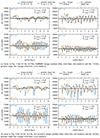 |
Fig. A.1. Period spacing patterns for the PyMMAMS and fast accretion merger products and their respective genuine single stars. |
All Figures
|
Fig. 1. HRD with MS evolutionary tracks for the 16.9 M⊙ 3D MHD merger product (black dashed line) and the 17.4 M⊙ genuine single star (green solid line). The grey and lime-coloured horizontal markers indicate different evolutionary stages, using the central hydrogen mass fraction Xc as a proxy for the evolutionary age, for the merger product and genuine single star, respectively. |
| In the text | |
|
Fig. 2. Evolution of the propagation diagrams (odd rows) and hydrogen mass fraction X profiles (even rows) for the 16.9 M⊙ 3D MHD merger product (solid lines) and the 17.4 M⊙ genuine single star (dashed lines). Each panel is labelled with the corresponding central hydrogen mass fractions of the merger product and the genuine single star. |
| In the text | |
|
Fig. 3. Comparison between the buoyancy travel time Π0 of the 16.9 M⊙ 3D MHD merger product (blue line) and the 17.4 M⊙ genuine single star (red line) as a function of their respective central hydrogen mass fractions Xc (panel a). Panel b shows the absolute differences in Π0, Δ(Π0)=Π0, single−Π0, merger. The error bar in panel b shows σΔP. |
| In the text | |
|
Fig. 4. Period spacing patterns for ℓ=1 g modes without rotation for the 16.9 M⊙ 3D MHD merger product (blue solid lines, dot markers) and the 17.4 M⊙ genuine single star (orange solid lines, cross markers) at different evolutionary stages. The horizontal solid black and dashed grey lines indicate the values of the asymptotic period spacing values Πℓ=1 for the merger product and genuine single star, respectively. The |
| In the text | |
|
Fig. 5. Period spacing patterns (PSPs) for (ℓ, m)=(1, ±1) and (ℓ, m)=(2, ±2) g modes with rotation rates of Ω/Ωc=0.10−0.30 (panels a–d) and Ω/Ωc=0.40−0.60 (panels e–h) for the 16.9 M⊙ 3D MHD merger product and the 17.4 M⊙ genuine single star at Xc, merger=0.50 and Xc, single=0.51, respectively. The black, blue, and grey lines with dot markers correspond to the merger product's PSPs, while the red, orange, and gold lines with cross markers correspond to the PSPs of the genuine single star. The PSPs are shown in the inertial (observer's) frame. |
| In the text | |
|
Fig. 6. Differences between the quadratic function fits of the PSPs for prograde modes shown in Fig. 5 for Ω/Ωc=0.10−0.30 (top) and Ω/Ωc=0.40−0.60 (bottom). The solid and dashed lines show the differences for the (ℓ, m)=(1, 1) and (ℓ, m)=(2, 2) modes, respectively. The horizontal red line shows the average value of σΔP from observations of SPB pulsators. |
| In the text | |
|
Fig. 7. Frequencies and radial orders np of ℓ=1 and ℓ=2 p modes with np≤4 for the 16.9 M⊙ 3D MHD merger product (blue and light-blue markers) and the 17.4 M⊙ genuine single star (red and orange markers) at different evolutionary stages, in the absence of rotation. The models at Xc=0.01 and Xc=0.10 are absent because of the lack of pure p modes at these evolutionary stages. The dot and cross markers show the value of the radial order np for the ℓ=1 and ℓ=2 modes, respectively. The dotted and dash-dotted lines are drawn to accentuate the frequency differences and improve the legibility of the frequency values. |
| In the text | |
|
Fig. 8. Absolute differences between the 17.4 M⊙ genuine single star's p-mode frequencies |
| In the text | |
|
Fig. 9. HRD with the evolutionary tracks of the 16.9 M⊙ merger product computed with the 3D MHD simulation (MHD, black dashed line), entropy sorting (ES, red dashed line), PyMMAMS (PM, blue dashed line), and fast accretion (FA, indigo dashed line). The corresponding 17.4 M⊙, 17.15 M⊙, 17.0 M⊙, and 16.9 M⊙ genuine single stars evolutionary tracks are drawn with grey, orange, cyan, and magenta solid lines, respectively. |
| In the text | |
|
Fig. 10. Comparison between the buoyancy travel time Π0 for the 16.9 M⊙ 3D MHD (MHD, black line), entropy-sorted (ES, red line), PyMMAMS (PM, blue line), and fast accretion (FA, indigo line) merger products (panel a), and the absolute differences Δ(Π0)=Π0, single−Π0, merger with their respective genuine single star models (panel b). The error bar in panel b shows the σΔP. |
| In the text | |
|
Fig. 11. Same as Fig. 4 but for the 16.9 M⊙ entropy sorted merger product (blue solid lines, dot markers) and the 17.15 M⊙ genuine single star (orange solid lines, cross markers). |
| In the text | |
|
Fig. 12. Mode frequencies and radial orders np for (ℓ, m)=(1, 0) and (ℓ, m)=(2, 0) p modes in the absence of rotation at Xc, merger=0.50 for the entropy-sorted (ES), PyMMAMS (PM), and fast accretion (FA) merger product models and their corresponding genuine single-star models. In the top three panels, the colour, line, and marker conventions are the same as in Fig. 7. The bottom panel shows the (ℓ, m)=(1, 0) p mode frequencies for the 3D MHD, entropy-sorted, PyMMAMS, and fast accretion models together. |
| In the text | |
|
Fig. 13. Absolute differences between the 17.4 M⊙, 17.15 M⊙, 17.0 M⊙, and 16.9 M⊙ genuine single star's p mode frequency |
| In the text | |
|
Fig. 14. Values of Πℓ=1=Π1 for the 3D MHD merger product at Xc=0.50 (cross marker, |
| In the text | |
|
Fig. A.1. Period spacing patterns for the PyMMAMS and fast accretion merger products and their respective genuine single stars. |
| In the text | |
Current usage metrics show cumulative count of Article Views (full-text article views including HTML views, PDF and ePub downloads, according to the available data) and Abstracts Views on Vision4Press platform.
Data correspond to usage on the plateform after 2015. The current usage metrics is available 48-96 hours after online publication and is updated daily on week days.
Initial download of the metrics may take a while.