© The Authors 2024

1. Introduction

The transport of angular momentum and chemical elements in stellar radiative zones is a key issue in modern stellar evolution theory. Purely hydrodynamical models fail to account for all the observational constraints; in particular, they are not efficient enough to reproduce the core rotation rates of red giant or intermediate-mass stars measured by seismology (Marques et al. 2013; Ceillier et al. 2013; Ouazzani et al. 2019). Models involving magnetic fields are a promising way of solving this angular momentum transport problem (Gough & McIntyre 1998; Fuller et al. 2019; Gouhier et al. 2022). However, observational constraints on the strength and topology of radiative zone magnetic fields are rare, limiting our ability to test these models.

Spectropolarimetry enables magnetic field measurements at the surface of stars with a radiative envelope. It was found that 5–10% of intermediate-mass and massive main-sequence stars have detectable magnetic fields. The vast majority of them are strong (>100 Gauss) and stable in time, and have a simple large scale topology (Aurière et al. 2007; Donati & Landstreet 2009; Wade et al. 2016), whereas very weak (∼1 Gauss) fields have been detected on a few very bright intermediate-mass stars (Lignières et al. 2014; Blazère et al. 2016). Asteroseismology has recently provided constraints on internal magnetic fields. First, the absence of the dipolar mixed gravito-acoustic modes in the oscillation spectrum of a fraction (∼20%) of red giant stars has been interpreted as due to strong magnetic fields in their radiative core (Fuller et al. 2015; Stello et al. 2016). Accordingly, if magnetic fields exceed a certain limit, gravity waves transform into short-wavelength Alfvèn waves that soon get dissipated (Lecoanet et al. 2017; Rui & Fuller 2023). It has nevertheless been argued that this interpretation is incompatible with the seismic properties of stars with weakly depressed dipolar mixed modes (Mosser et al. 2017). Second, a clear signature of magnetic fields, the asymmetry of the ℓ = 1 triplet, has been discovered in the oscillation spectrum of 13 red giant stars. This data, together with a theoretical description of the effects of an arbitrary magnetic field on these oscillation modes, enabled the measurement of the strength of the radial component of the magnetic field in the vicinity of the H-burning shell of these stars, and constraints on their topology (Li et al. 2022, 2023). A related seismic signature, the deviation from the uniform period spacing of gravity modes (hereafter g modes), led to the detection of core magnetic fields in 11 more red giant stars (Deheuvels et al. 2023).

Beyond red giants, seismic signatures of magnetic fields can of course be searched in other pulsating stars. γ Doradus (γ Dor) stars are good candidates because (i) they oscillate in the low-frequency range, which is most affected by magnetic fields, (ii) their modes are gravity and Rossby modes, which are sensitive to the radiative layers just outside the convective core where a magnetic field is most probably generated by a convective dynamo, and (iii) these gravity and Rossby modes are identified in more than 600 γ Dor stars (Li et al. 2020) observed by Kepler (Borucki et al. 2010) and in about 60 γ Dor stars (Garcia et al. 2022) observed by TESS (Transiting Exoplanet Survey Satellite, Ricker et al. 2015). However, the two seismic diagnostics available to search for magnetic fields in slowly rotating red giants, namely the asymmetry of the ℓ = 1 triplet and the deviation from the g-mode uniform period spacing, are not relevant for rapidly rotating stars such as γ Dor stars. A theoretical analysis of the effects of an arbitrary magnetic field in a rapidly rotating star is therefore necessary to search for and interpret potential magnetic seismic signatures in γ Dors.

The effects of a magnetic field on oscillation modes were first considered for acoustic modes in Unno et al. (1989), Gough & Thompson (1990). Both the magnetic field and the rotation were assumed to be small enough to be treated perturbatively. This approach was later applied to high-order g modes, including mixed gravito-acoustic modes. In these studies, the poloidal magnetic field has been assumed to take the simple form of a dipolar field either aligned (Hasan et al. 2005; Gomes & Lopes 2020; Bugnet et al. 2021; Mathis et al. 2021) or inclined (Loi 2021) with respect to the rotation axis. In Li et al. (2022), we extended to an arbitrary field the perturbative analysis of magnetic and rotation effects on g modes. This extension is significant as we do not want seismic measurements of a magnetic field to depend on an a priori assumption about the magnetic field topology.

In γ Dor stars, the rotation cannot be treated with a perturbative method, as the Coriolis force significantly affects the g modes and induces new modes such as the Rossby modes (hereafter the r modes). A well-known approximation, the traditional approximation of rotation (TAR), allows Coriolis effects to be taken into account while keeping the eigenvalue problem separable in the spherical coordinates. Although the TAR has its limitations (Friedlander 1987; Gerkema & Shrira 2005; Ballot et al. 2012; Ouazzani et al. 2017, 2020), it is most often accurate and has been successful in identifying oscillation modes and measuring core rotation rates in γ Dor stars (Bedding et al. 2015; Van Reeth et al. 2015, 2016; Christophe et al. 2018; Li et al. 2019, 2020). The magnetic effects on TAR gravito-inertial modes have already been studied in the case of dipolar poloidal magnetic fields either aligned (Prat et al. 2019) or inclined (Prat et al. 2020) with respect to the rotation axis. In both studies, frequency shifts induced by the dipolar magnetic field have been computed for one particular stellar model. In the present paper, we extend these works (i) by considering an arbitrary magnetic field and (ii) by deriving approximate analytical formulae relating the magnetic frequency shifts to a weighted average of the internal magnetic field, the rotation rate, and stellar structure properties for the modes that are most frequently identified in γ Dor stars. We then propose simple methods to search for magnetic seismic signatures and potentially measure magnetic fields in the frequency spectra of γ Dor or SPB stars.

The paper is organised as follow: the formula of the frequency shift induced by an arbitrary magnetic field on high-order gravito-inertial modes is derived in Sect. 2. In Sect. 3, properties of the magnetic frequency shift are studied for the modes observed in γ Dor: approximate analytical formulas are derived and tested (Sect. 3.1), the magnetic shift of the different modes are compared to help detect magnetic signature in observed spectra (Sect. 3.2), and methods to detect magnetic signatures are tested on synthetic spectra (Sect. 3.3). In Sect. 4, the results are summarised and discussed.

2. Derivation of the magnetic shift

Time-harmonic, ∝exp(iωt), small perturbations of a magnetic and uniformly rotating star are solutions of the following eigenvalue problem:

$$\begin{array}{c}\hfill {\omega }^2\mathit{\xi }=2i\omega \mathbf{\Omega }\wedge \mathit{\xi }+{\mathcal{L}}_0(\mathit{\xi })+{\mathcal{L}}_{\mathrm{L}}(\mathit{\xi }),\end{array}$$(1)

where ξ is the displacement vector, 2iωΩ ∧ ξ is the Coriolis force term, and ℒ₀ is a linear operator,

$$\begin{array}{c}\hfill {\mathcal{L}}_0(\mathit{\xi })={\rho }^{-1}\mathbf{\nabla }p\prime +\mathbf{\nabla }\psi \prime +{\rho }^{-1}\mathbf{\nabla }\psi \rho \prime ,\end{array}$$(2)

that has the same form as in a non-rotating, non-magnetic star, with ρ and ψ the equilibrium density and gravitational potential, and p′, ρ′, and ψ′ the perturbations to pressure, density, and gravitational potential. ℒ_L(ξ) is the linear operator associated with the Lorentz force,

$$\begin{array}{c}\hfill {\mathcal{L}}_{\mathrm{L}}(\mathit{\xi })=-\frac{1}{\rho {\mu }_0}[(\mathbf{\nabla }\times \mathit{B}\prime )\times \mathit{B}+(\mathbf{\nabla }\times \mathit{B})\times \mathit{B}\prime ]-\frac{\mathbf{\nabla }·(\rho \mathit{\xi })}{{\rho }^2{\mu }_0}[(\mathbf{\nabla }\times \mathit{B})\times \mathit{B}],\end{array}$$(3)

with B the star magnetic field, B′=∇ × (ξ × B) the Eulerian perturbation to B, and μ₀ the magnetic permeability (e.g. Li et al. 2022).

We performed a first-order perturbative analysis of the effects of a magnetic field, assuming ‖ℒ_L(ξ)‖ ≪ ‖ℒ_o(ξ) + 2iωΩ∧ξ‖. The oscillation frequency and the displacement vector were written as the sum of unperturbed and perturbed quantities, that is, ω = ω₀ + ω₁, ξ = ξ₀ + ξ₁, with ω₁ ≪ ω₀ and ∥ξ₁ ≪ ξ₀∥, and inserted into Eq. (1). At zero order, the system reduces to the eigenvalue problem governing the oscillations of a rotating non-magnetic star:

$$\begin{array}{c}\hfill {\omega }_0^2{\mathit{\xi }}_0-2i{\omega }_0\mathbf{\Omega }\wedge {\mathit{\xi }}_0={\mathcal{L}}_0({\mathit{\xi }}_0).\end{array}$$(4)

In the low-frequency domain, this problem can simplified using the TAR (Eckart 1960; Lee & Saio 1997; Townsend 2003). In this framework, the centrifugal force, the perturbations of the gravitational potential, and the latitudinal component of the rotation vector, Ω, are neglected. The eigenvalue problem then becomes separable in the spherical coordinates so that the eigenfunctions, ξ₀, can be written as

$$\begin{array}{c}\hfill {\mathit{\xi }}_0=e^{i(m\varphi +{\omega }_{0}t)}({\xi }_r(r)H_r(\theta ){\mathit{e}}_r+{\xi }_h(r)H_{\theta }(\theta ){\mathit{e}}_{\theta }+i{\xi }_h(r)H_{\varphi }(\theta ){\mathit{e}}_{\varphi }),\end{array}$$(5)

where the variations in latitude are given by the three functions, H_r, H_θ, H_ϕ, which are known as Hough functions. The radial Hough function, H_r, is the solution of Laplace’s tidal equation,

$$\begin{array}{c}\hfill {\mathcal{L}}_{\mathrm{T}}(H_r)+\mathrm{\Lambda }{H}_r=0\end{array}$$(6)

with

$$\begin{array}{cc}\hfill {\mathcal{L}}_{\mathrm{T}}(H_r)& =\frac{\mathrm{d}}{\mathrm{d}\mu }\left[\frac{1-{\mu }^2}{(1-s^2{\mu }^2)}\frac{\mathrm{d}}{\mathrm{d}\mu }{H}_r\right]\hfill \\ \hfill & -\frac{1}{1-s^2{\mu }^2}(\frac{m^2}{1-{\mu }^2}+ms\frac{1+s^2{\mu }^2}{1-s^2{\mu }^2})H_r,\hfill \end{array}$$

where μ = cos θ, θ is the colatitude, and $s=\frac{2\mathrm{\Omega }}{{\omega }_0}$ is the spin parameter. For a non-rotating star, the eigenvalues, Λ, are equal to ℓ(ℓ + 1) for all azimuthal numbers, −ℓ≤m ≤ ℓ, and the eigenfunctions are a linear combination of the 2ℓ+1 spherical harmonics $Y_{\mathcal{l}}^m$, ℓ denoting the degree of the spherical harmonic. The m-degeneracy is lifted in a rotating star. The eigenvalues, Λ_ℓ, m(s), and eigenfunctions, $H_r^{\mathcal{l},m}(\theta ,s)$, of Laplace’s tidal equation that correspond to g modes at a vanishing rotation are labelled with ℓ and m. For the r modes that only exist in rotating stars, a different label, k, is used instead of ℓ. In the following, the ℓ, m, s or k, m, s dependence will most often be implicit to ease the reading. The horizontal Hough functions, H_θ, H_ϕ, can be derived from H_r through Eqs. (B.1) and (B.2).

In the radial direction, the eigenvalue problem is identical to the radial eigenvalue problem of the non-rotating case except that ℓ(ℓ + 1) is replaced by Λ. Since γ Dor stars oscillate in high-order modes, the Wentzel–Kramers–Brillouin (WKB) solution of the radial eigenvalue problem provides a good approximate solution as long as the mode radial wavelength is much shorter than the scales of variation in the star structure. It reads:

$$\begin{array}{c}\hfill \frac{2\pi }{{\omega }_0}=\frac{{\mathrm{\Pi }}_0(n+{ϵ}_g)}{\sqrt{\mathrm{\Lambda }}},\end{array}$$(7)

with

$$\begin{array}{c}\hfill {\mathrm{\Pi }}_0=\frac{2{\pi }^2}{{\int }_{r_{\mathrm{i}}}^{r_{\mathrm{o}}}\frac{N}{r}\mathrm{d}r}·\end{array}$$(8)

r_i and r_o are the inner and outer boundaries of the g-mode cavity, n is the mode radial order, and N(r) is the Brunt-Väisälä frequency. As Λ depends on s, Eq. (7) is an implicit equation for s. For a given (ℓ,m), it relates s with n. In the following, we shall also use the WKB solution for the horizontal component of the displacement vector, ξ_h ∝ ρ^−1/2r^−3/2N^1/2Λ^−1/4sin(Φ(r))ω^−3/2, with $\mathrm{\Phi }(r)={\int }_{r_i}^r{k}_r-\pi /4\text{d}r$ where $k_r^2=\frac{N^2}{{\omega }_0^2}\frac{\mathrm{\Lambda }}{r^2}$ represents the square of the local radial wavelength.

At first order, the eigenvalue problem, Eq. (1), corresponds to the following eigenvalue problem for the perturbed frequency, ω₁, and the perturbed eigenfunctions, ξ₁:

$$\begin{array}{c}\hfill {\omega }_1[2{\omega }_0{\mathit{\xi }}_0-2i\mathbf{\Omega }\wedge {\mathit{\xi }}_0]={\mathcal{L}}_{\mathrm{L}}({\mathit{\xi }}_0)-{\omega }_0^2{\mathit{\xi }}_1+2i{\omega }_0\mathbf{\Omega }\wedge {\mathit{\xi }}_1+{\mathcal{L}}_0({\mathit{\xi }}_1).\end{array}$$(9)

As discussed in Gough & Thompson (1990) and Mathis & Bugnet (2023), the modification of the hydrostatic equilibrium by the magnetic field is neglected as its effect on low-frequency g modes is negligible compared to the effect of the perturbed Lorentz force ℒ_L(ξ₀). Taking the scalar product of this equation with ξ₀ and using the self-adjoint character of the operator, ℒ₀ + 2iωΩ∧, we obtain

$$\begin{array}{c}\hfill {\omega }_1=\frac{⟨{\mathit{\xi }}_0,{\mathcal{L}}_{\mathrm{L}}({\mathit{\xi }}_0)⟩}{2{\omega }_0⟨{\mathit{\xi }}_0,{\mathit{\xi }}_0⟩-⟨{\mathit{\xi }}_0,2i\mathbf{\Omega }\wedge {\mathit{\xi }}_0⟩},\end{array}$$(10)

where the inner product is

$$\begin{array}{c}\hfill \langle \mathit{f},\mathit{g}\rangle ={\displaystyle {\int }_V\rho {\mathit{f}}^{\ast }·\mathit{g}\mathrm{d}V,}\end{array}$$(11)

with V being the star volume. This general expression of the magnetic shift was already derived in Prat et al. (2019).

In the case of slowly rotating stars, Hasan et al. (2005) showed that the expression of the magnetic shift can be significantly simplified for low-frequency g modes provided the magnetic field varies over scales larger than the mode radial wavelength. As detailed in Appendix A, this simplification also holds for the low-frequency gravito-inertial modes as long as B_ϕ/B_r ≪ (N/ω₀) and B_θ/B_r ≪ (N/2Ω)^1/2(N/ω₀)^1/2. In this regime, the magnetic frequency shift only involves the horizontal displacements and the radial field component,

$$\begin{array}{c}\hfill {\omega }_1=\frac{1}{2{\mu }_0{\omega }_0}\frac{{\int }_{r_i}^{r_o}{\int }_0^{\pi }{|\frac{\partial }{\partial r}\left(r{\xi }_h\right)|}^2(H_{\theta }^2+H_{\varphi }^2){⟨B_r^2⟩}_{\varphi }sin\theta \mathrm{d}\theta \mathrm{d}r}{{\int }_{r_i}^{r_o}\rho r^2{\xi }_h^2\mathrm{d}r{\int }_0^{\pi }(H_{\theta }^2+H_{\varphi }^2-\frac{2\mathrm{\Omega }}{{\omega }_0}{H}_{\theta }{H}_{\varphi }cos\theta )sin\theta \mathrm{d}\theta },\end{array}$$(12)

where

$$\begin{array}{c}\hfill {⟨B_r^2⟩}_{\varphi }(r,\theta )=\frac{1}{2\pi }{\displaystyle {\int }_0^{2\pi }{B}_r^2(r,\theta ,\varphi )\mathrm{d}\varphi .}\end{array}$$(13)

This formula generalises to an arbitrary magnetic field the expression obtained by Prat et al. (2019, 2020) for an oblique dipolar field. It is valid for low-frequency (or equivalently high-order) TAR gravito-inertial modes in a magnetic field that is not strongly dominated by its horizontal components.

Using the WKB solution for ξ_h(r) and the stationary phase approximation, the integral involving ξ_h(r) can be simplified as

$$\begin{array}{c}\hfill \frac{{\int }_{r_i}^{r_o}{|\frac{\partial }{\partial r}\left(r{\xi }_h(r)\right)|}^{2}f(r)\mathrm{d}r}{2{\int }_{r_i}^{r_o}\rho r^2{\xi }_h^2\mathrm{d}r}=\frac{\mathrm{\Lambda }}{2{\omega }_0^2}\frac{{\int }_{r_i}^{r_o}{\left(\frac{N}{r}\right)}^3\frac{f(r)}{\rho }\mathrm{d}r}{{\int }_{r_i}^{r_o}\frac{N}{r}\mathrm{d}r},\end{array}$$(14)

where f(r) is an arbitrary smooth function. The magnetic frequency shift then becomes

$$\begin{array}{cc}\hfill {\omega }_1& =\frac{1}{{\mu }_0}\frac{\mathrm{\Lambda }}{2{\omega }_0^3}\mathcal{I}\frac{{\int }_0^{\pi }(H_{\theta }^2+H_{\varphi }^2)sin\theta \mathrm{d}\theta }{{\int }_0^{\pi }(H_{\theta }^2+H_{\varphi }^2-\frac{2\mathrm{\Omega }}{{\omega }_0}{H}_{\theta }{H}_{\varphi }cos\theta )sin\theta \mathrm{d}\theta }\hfill \\ \hfill & \times {\int }_{r_i}^{r_o}{\int }_0^{\pi }{K}_r(r)K_{\theta }(\theta ){⟨B_r^2⟩}_{\varphi }sin\theta \mathrm{d}\theta \mathrm{d}r,\hfill \end{array}$$(15)

where

$$\begin{array}{cc}\hfill \mathcal{I}& =\frac{{\int }_{r_i}^{r_o}\frac{1}{\rho }{\left(\frac{N}{r}\right)}^3\mathrm{d}r}{{\int }_{r_i}^{r_o}\frac{N}{r}\mathrm{d}r}\hfill \end{array}$$(16)

$$\begin{array}{cc}\hfill K_r(r)& =\frac{\frac{1}{\rho }{\left(\frac{N}{r}\right)}^3}{{\int }_{r_i}^{r_o}\frac{1}{\rho }{\left(\frac{N}{r}\right)}^3\mathrm{d}r}\hfill \end{array}$$(17)

$$\begin{array}{cc}\hfill K_{\theta }(\theta )& =\frac{H_{\theta }^2+H_{\varphi }^2}{{\int }_0^{\pi }(H_{\theta }^2+H_{\varphi }^2)sin\theta \mathrm{d}\theta }·\hfill \end{array}$$(18)

The term ℐ depends on the stellar structure within the oscillating cavity, and ${\langle B_r^2\rangle }_{\varphi }$ is the azimuthal average of $B_r^2$, while K_r and K_θ are, respectively, radial and latitudinal weight functions, as they verify that ${\int }_{r_i}^{r_o}{K}_r(r)\hspace{0.17em}\text{d}r={\int }_0^{\pi }{K}_{\theta }(\theta )sin\theta \hspace{0.17em}\text{d}\theta =1$.

In a non-rotating star, this expression reduces to

$$\begin{array}{c}\hfill {\omega }_1(s=0)=\frac{\mathcal{I}}{2{\mu }_0}\frac{\ell (\ell +1)}{{\omega }_0^3}{\displaystyle {\int }_{r_i}^{r_o}{K}_r(r){\int }_0^{\pi }{K}_{\theta }(\theta ){⟨B_r^2⟩}_{\varphi }sin\theta \mathrm{d}\theta \mathrm{d}r,}\end{array}$$(19)

where

$$\begin{array}{cc}\hfill K_{\theta }(\theta )& =\frac{{\left(\frac{\partial {\widehat{Y}}_{\ell }^m}{\partial \theta }\right)}^2+\frac{m^2}{{sin}^2\theta }{\left({\widehat{Y}}_{\ell }^m\right)}^2}{{\int }_0^{\pi }[{\left(\frac{\partial {\widehat{Y}}_{\ell }^m}{\partial \theta }\right)}^2+\frac{m^2}{{sin}^2\theta }{\left({\widehat{Y}}_{\ell }^m\right)}^2]sin\theta \mathrm{d}\theta }\hfill \\ \hfill & =\frac{2\pi }{\ell (\ell +1)}[{\left(\frac{\partial {\widehat{Y}}_{\ell }^m}{\partial \theta }\right)}^2+\frac{m^2}{{sin}^2\theta }{\left({\widehat{Y}}_{\ell }^m\right)}^2],\hfill \end{array}$$(20)

where ${\widehat{Y}}_{\ell }^m(\theta )$ is the latitudinal part of the spherical harmonic of degree, ℓ, and the azimuthal number, m, defined as $Y_{\ell }^m(\theta ,\varphi )={\widehat{Y}}_{\ell }^m(\theta )e^{im\varphi }$. As was expected, we recovered the diagonal terms of the magnetic matrix derived by Li et al. (2022). We note that the non-diagonal terms of the magnetic matrix are not relevant for the rapidly rotating stars considered in the present study. Indeed, they arise in slowly rotating from the coupling of the nearly degenerate components of the multiplet.

To analyse the properties of the magnetic frequency shift in a rotating star, we found it convenient to rewrite Eq. (12) as

$$\begin{array}{c}\hfill {\omega }_1=\frac{\mathcal{I}}{2{\mu }_0}\frac{F(s)}{{\omega }_0^3}{T}_B(s)⟨B_r^2⟩,\end{array}$$(21)

where we introduced two dimensionless factors,

$$\begin{array}{c}\hfill F(s)=\mathrm{\Lambda }\frac{{\int }_0^{\pi }(H_{\theta }^2+H_{\varphi }^2)sin\theta \mathrm{d}\theta }{{\int }_0^{\pi }(H_{\theta }^2+H_{\varphi }^2-s{H}_{\theta }{H}_{\varphi }cos\theta )sin\theta \mathrm{d}\theta },\end{array}$$(22)

and

$$\begin{array}{c}\hfill T_B(s)=\frac{{\int }_0^{\pi }{K}_{\theta }(\theta ){⟨B_r^2⟩}_{\varphi ,r}sin\theta \mathrm{d}\theta }{⟨B_r^2⟩},\end{array}$$(23)

and two different averages of $B_r^2$,

$$\begin{array}{c}\hfill {⟨B_r^2⟩}_{\varphi ,r}(\theta )={\displaystyle {\int }_{r_i}^{r_o}{K}_r(r){⟨B_r^2⟩}_{\varphi }\mathrm{d}r,}\end{array}$$(24)

the average of $B_r^2$ in the azimuthal and radial directions, the average in the radial direction being weighted by K_r(r) and performed between the inner and outer radii of the mode cavity, and

$$\begin{array}{c}\hfill ⟨B_r^2⟩=\frac{1}{4\pi }{\displaystyle {\int }_{r_i}^{r_o}{K}_r(r){\int }_0^{\pi }{\int }_0^{2\pi }{B}_r^{2}sin\theta \mathrm{d}\theta \mathrm{d}\varphi \mathrm{d}r,}\end{array}$$(25)

the average of $B_r^2$ performed over the whole volume of the mode cavity, with a K_r weight in the radial direction.

The factor, F, depends on the mode, that is on ℓ (or k), m, and s, but not on the magnetic field or the stellar structure. The factor, T_​​B, is a weighted average of $B_r^2$ scaled by $\langle B_r^2\rangle$. It depends on the field topology but also on the mode through the latitudinal weight function, K_θ(θ). The product, $\mathcal{I}⟨B_r^2⟩$, depends on the stellar structure and on the mode considered through the radii of the mode cavity.

3. Analysis of the magnetic frequency shift for the modes identified in γ Dor stars

In the following, we focus our analysis on the four types of mode that are most frequently identified in γ Dor stars: the two sectoral prograde g modes (also named Kelvin modes), (ℓ = 1, m = −1) and (ℓ = 2, m = −2), the r mode labelled (k = −2, m = 1), and the zonal dipolar g mode (ℓ = 1, m = 0). What is actually identified in these stars are frequency patterns formed by different radial orders, n, of these modes. Among the 611 γ Dors analysed by Li et al. (2020), 594 stars show a frequency pattern of (ℓ,m) = (1, −1) modes, 172 a pattern of (ℓ,m) = (2, −2) modes, and 110 a pattern of (k = −2, m = 1) modes, while 29 stars show a pattern of (ℓ,m) = (1, 0) modes, although only 11 stars among them have a typical γ Dor fast rotation (P_rot ∼ 1 day). Retrograde dipolar modes have also been observed but only in slowly rotating stars and will not be considered here. The radial orders are rather high and the patterns cover a large interval of radial orders. Indeed, for the two prograde sectoral modes, the radial order distribution has a median value of n ∼ 50 and a mean pattern length of 30 radial orders. For the (k = −2, m = 1) r modes, the median is lower, n ∼ 36, but the mean pattern length is also 30. Similar radial orders translate into different spin parameter intervals for the different modes. Indeed, for the prograde dipolar mode (ℓ = 1, m = −1), the spin parameter distribution peaks at s = 5 and goes up to ∼20, while it peaks at s = 2.5 and goes up to ∼10 for the quadrupolar sectoral modes (ℓ = 2, m = −2). The interval of (k = −2, m = 1) r mode spin parameters range from 6 to ∼35, with a peak at s ∼ 9. And among the 11 fast rotating stars with zonal dipolar g modes (ℓ = 1, m = 0), the spin parameter ranges from ∼1 to ∼2.5.

For a given frequency pattern, that is, for a given star and a fixed (ℓ,m) or (k, m), the magnetic frequency shift varies with the spin parameter, s (or equivalently the radial order n). In Sect. 3.1, we study these variations and derive and test approximate analytical formulas for the frequency shift of the selected modes. In Sect. 3.2, we compare the magnetic shifts of these different modes and study a simple seismic diagnostic of the presence of magnetic fields when both (ℓ,m) = (1, −1) and (ℓ,m) = (2, −2) modes are present. In Sect. 3.3, we construct synthetic frequency patterns affected by magnetic fields and test simple methods of detecting magnetic signatures.

3.1. Variations in the magnetic frequency shift with the spin parameter

We successively studied the terms F, T_​​B, and $\mathcal{I}{⟨B_r^2⟩}_{\varphi ,r}$ involved in the expression Eq. (21) of the frequency shift. To do so, we used both numerical and analytical calculations, the latter being valid in the s ≫ 1 limit. This allowed us to derive and test approximate analytical formulas of the magnetic frequency shifts.

3.1.1. The F factor

We recall that for a given (ℓ,m) the F factor defined by Eq. (22) only depends on s. The numerical determination of F requires us to compute Λ(s) and H_r(θ, s) from Laplace’s tidal equation, to derive H_θ and H_ϕ from (Λ(s), H_r(θ, s)), and to compute the integrals involved in the F factor. These calculations are detailed in Appendix B. Approximate analytical expressions of F can also be obtained from analytic expressions of Λ and the Hough functions valid in the high-s limit (Townsend 2003). These calculations are detailed in Appendices C.1 and C.2.

Figure 1 displays both the numerical and the asymptotic forms of the factor, F, for the two prograde sectoral modes, (ℓ,m) = (1, −1) and (ℓ,m) = (2, −2), and for the r mode, (k, m) = (−2, 1). As was expected, F(0) = ℓ(ℓ+1) for the two g modes when the rotation vanishes. As s increases from 0 to 20, F decreases by a factor of two for (ℓ,m) = (1, −1) and by a factor of 2/3 for (ℓ,m) = (2, −2). F actually approaches a constant value for large spin parameters, F ∼ 1 for (ℓ,m) = (1, −1) and F ∼ 4 for (ℓ,m) = (2, −2). This is in agreement with the analytical study that shows that lim_{s → ∞}F_|m|,m = lim_{s → ∞}Λ_|m|,m = m² for these two modes. More precisely, the asymptotic forms are F_1, −1(s) = 1 + 1/(4s)+1/(8s²) and F_2, −2(s) = 4(1 + 1/(8s)+1/(32s²)) and, as shown on Fig. 1, they provide very good approximations when, say, s ≳ 2.5.

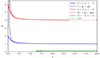Fig. 1. F factor of the prograde sectoral modes, ℓ = 1, m = −1 (blue), and ℓ = 2, m = −2 (red), and of the r mode, k = −2, m = 1 (green), as a function of the spin parameter, s. The asymptotic s ≫ 1 forms of the F factor are also plotted (dashed lines).

The r mode, (k, m) = (−2, 1), only exists for spin parameters above s = 6 (Lee & Saio 1997). Its F factor vanishes there, as Λ_−2, 1(s = 6) = 0. As for the two previous modes, F_−2, 1 approaches Λ_−2, 1 ≈ 1/9 for large s. For this mode, the high-s analytical form is simply F_−2, 1 ≈ 1/9. For the zonal dipolar mode, (ℓ,m) = (1, 0), the numerical and analytical F factors are displayed in Fig. C.1. The F factor is very well approximated by its asymptotic form, F_1, 0(s) = (3/2)s².

3.1.2. The T_​B factor

The factor, T_​​B, defined by Eq. (23) is a weighted latitudinal integral of ${\langle B_r^2\rangle }_{\varphi ,r}(\theta )$ normalised by $\langle B_r^2\rangle$. Here, we analyse its variations with the spin parameter and the magnetic field topology for the same four modes. For a given mode, the weight function, K_θ(θ), only depends on the spin parameter. Figure 2 shows the latitudinal profile of the weight function of the four modes computed at s = [0.1, 1, 8, 15]. We observe that all the weight functions concentrate towards the equator as s increases. This is a consequence of the well-known tendency of the Hough functions to equatorial concentration (Lee & Saio 1997; Townsend 2003). We also observe that at a fixed s this effect is more or less important, depending on the mode. The axisymmetric dipolar mode is the most concentrated, followed by the (ℓ,m) = (2, −2) mode, the (ℓ,m) = (1, −1) mode, and finally the r mode, which is not yet equatorially concentrated at s = 8. This behaviour is in qualitative agreement with the high-s asymptotic form of the Hough functions (Townsend 2003) that indicate that the half-width of H_θ are 1/s for the (ℓ,m) = (1, 0) mode, $\sqrt{3/(-ms)}$ for the (ℓ,m) = (2, −2) and (ℓ,m) = (1, −1) modes, and $\sqrt{3/(s-1)}$ for the r-mode.

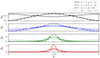Fig. 2. Latitudinal weight functions, Kθ, of the two prograde sectoral modes, ℓ = 1, m = −1 (continuous lines) and ℓ = 2, m = −2 (dashed lines), the zonal dipolar mode, ℓ = 1, m = 0 (dash-dotted lines), and the r mode, k = −2, m = 1 (dotted lines), at four different spin parameters, s = 0.1 (black), s = 1 (blue), s = 8 (green), and s = 15 (red).

As a consequence of the equatorial concentration, the K_θ average of $B_r^2$ is increasingly weighted towards the equator so that for very large spin parameters we expect $T_B\approx {\langle B_r^2\rangle }_{\varphi ,r}(\theta =\pi /2)/\langle B_r^2\rangle$. In this limit, T_​​B is thus constant with s and identical for all the modes. From a Taylor expansion of $B_r^2$ at the equator, we can determine how T_​​B(s) tends towards ${\langle B_r^2\rangle }_{\varphi ,r}(\theta =\pi /2)/\langle B_r^2\rangle$ (see details in Appendix C.3). For the two sectoral prograde modes and the r mode, we obtain

$$\begin{array}{c}\hfill T_B^{\ell ,m}(s)⟨B_r^2⟩={⟨B_r^2⟩}_{\varphi ,r}(\theta =\pi /2)+\frac{1}{\alpha s}\frac{{\mathrm{d}}^2{⟨B_r^2⟩}_{\varphi ,r}}{\mathrm{d}{\theta }^2}(\theta =\pi /2),\end{array}$$(26)

with α = 4 for (ℓ = 1, m = −1), α = 8 for (ℓ = 2, m = −2), and α = 4/3 for (k = −2, m = 1), while, for the dipolar mode axisymmetric,

$$\begin{array}{c}\hfill T_B^{1,0}(s)⟨B_r^2⟩={⟨B_r^2⟩}_{\varphi ,r}(\theta =\pi /2)+\frac{5}{12s^2}\frac{{\mathrm{d}}^2{⟨B_r^2⟩}_{\varphi ,r}}{\mathrm{d}{\theta }^2}(\theta =\pi /2).\end{array}$$(27)

This approximation requires that near the equator ${\langle B_r^2\rangle }_{\varphi ,r}(\theta )$ varies on scales larger than the width of the weight function, K_θ. To the first two orders in the 1/s expansion, T_​​B depends on ${\langle B_r^2\rangle }_{\varphi ,r}$ and its second derivative at the equator. The next order would involve the fourth derivative of ${\langle B_r^2\rangle }_{\varphi ,r}$ at the equator. These expressions also indicate that the convergence towards ${\langle B_r^2\rangle }_{\varphi ,r}(\theta =\pi /2)/\langle B_r^2\rangle$ is faster (∝1/s²) for the dipolar axisymmetric mode than for the other three modes (∝1/s).

To test these expressions, we computed T_​​B(s) for an oblique dipolar field. This is a favourable case since the field varies on large scales around the equator. If β denotes the inclination angle of the dipole with respect to the rotation axis, the radial component of the oblique dipole reads B_r(r, θ, ϕ) = B₀b(r)(cos θ cos β + sin θ cos ϕ sin β) (Prat et al. 2020). A straightforward calculation (see Appendix D) then yields

$$\begin{array}{cc}\hfill T_B(s)& =3{cos}^2\beta {\displaystyle {\int }_0^{\pi }{K}_{\theta }(\theta ,s){cos}^2\theta sin\theta \mathrm{d}\theta }\hfill \\ \hfill & +\frac{3}{2}{sin}^2\beta {\displaystyle {\int }_0^{\pi }{K}_{\theta }(\theta ,s){sin}^2\theta sin\theta \mathrm{d}\theta .}\hfill \end{array}$$(28)

Figure 3 shows both the numerical and analytical forms of T_​​B(s) for the four modes and for three inclination angles, β = 0° ,47° ,90°, of the oblique dipole. We find that the high-s asymptotic expressions provide good approximations above some spin parameters, say above s ≳ 5 for (ℓ,m) = (1, −1), s ≳ 2.5 for (ℓ,m) = (2, −2) and (ℓ,m) = (1, 0), and s ≳ 20 for (k, m) = (−2, 1). As for the F factor, the convergence is more or less rapid depending on the mode tendency to equatorial concentration. We also observe that, as expected, T_​​B(s) converges towards the same value, ${⟨B_r^2⟩}_{\varphi ,r}(\theta =\pi /2)/⟨B_r^2⟩=\frac{3}{2}{sin}^2\beta$, for all the modes.

Fig. 3. T​​B factors of the (ℓ,m) = [(1, −1),(2, −2),(1, 0)], (k, m) = (−2, 1) modes displayed as a function of their spin parameter for three different angles of the inclined dipolar field, β = 0° (blue), β = 47° (green), and β = 90° (red). The continuous lines correspond to the numerical results and the dashed lines to the approximate analytical solutions valid in the high-s limit.

3.1.3. The $\mathcal{I}{⟨{\mathit{B}}_{\mathit{r}}^2⟩}_{\varphi ,\mathit{r}}$ term

The magnetic frequency shift can also depend on s through the radii of the mode cavity. This dependency is contained in the product of the two terms ℐ and ${\langle B_r^2\rangle }_{\varphi ,r}$ :

$$\begin{array}{c}\hfill \mathcal{I}{⟨B_r^2⟩}_{\varphi ,r}=\frac{{\int }_{r_i}^{r_o}\frac{1}{\rho }{\left(\frac{N}{r}\right)}^3{⟨B_r^2⟩}_{\varphi }\mathrm{d}r}{{\int }_{r_i}^{r_o}\frac{N}{r}\mathrm{d}r}·\end{array}$$(29)

The inner and outer cavity radii being determined by the conditions ω₀ = Min(N, S), where $S=\frac{c_s}{r}\sqrt{\mathrm{\Lambda }}$ is the Lamb frequency and c_s the sound speed, they are likely to depend on the mode frequency, ω₀, and thus on s. The inner radius, r_i, remains very close to the outer radius of the convective core for high-order g modes though. This is due to the sharp increase in the Brunt-Väisälä frequency at the bottom of the radiative zone. Conversely, the outer radius, r_o, that is located in the radiative envelope of γ Dors does depend on the mode frequency. The vertical lines in Fig. 4 illustrate, in the case of the (ℓ,m) = (1, −1) mode, the variations in r_o as s takes three different values [2, 5, 15].

Fig. 4. Radial profile of $\frac{1}{\rho }{\left(\frac{N}{r}\right)}^3$ in c.g.s units for a M = 1.6 M⊙, R = 2.13 R⊙, Xc = 0.35 stellar model computed with the CESAM code. The outer radii, ro, of the oscillation cavity of (ℓ,m) = (1, −1) modes is shown by vertical lines for three different spin parameters, s = 2 (orange), s = 5 (green), and s = 15 (red).

The variation in the outer radius of the mode cavity does not affect significantly ${\int }_{r_i}^{r_o}N/r\hspace{0.17em}\text{d}r$, the denominator of $\mathcal{I}{⟨B_r^2⟩}_{\varphi ,r}$, because N/r peaks strongly near the bottom of the radiative zone. But it can affect the numerator, that is, the integral, ${\int }_{r_i}^{r_o}\frac{1}{\rho }{\left(\frac{N}{r}\right)}^3{⟨B_r^2⟩}_{\varphi }\mathrm{d}r$. Figure 4 indeed shows that $\frac{1}{\rho }{\left(\frac{N}{r}\right)}^3$ is dominant and increases rapidly in the star envelope up to the surface convective zone where N vanishes. Assuming a uniform magnetic field, Fig. 5 shows that this induces a sharp increase in $\mathcal{I}{⟨B_r^2⟩}_{\varphi ,r}$ between s ∼ 2 and s ∼ 6 for (ℓ,m) = (1, −1) modes. For higher spin parameters, r_o remains fixed at the bottom of the surface convective zone so that $\mathcal{I}{⟨B_r^2⟩}_{\varphi ,r}$ no longer varies with the spin parameter. Considering a dipole-like ∝1/r³ decrease in B_r within the envelope instead of a uniform field would not significantly modify this picture. Conversely, if the magnetic field decreases by various orders of magnitude between r_i and r_o, the variations in r_o will not affect the weighted integral of ${\langle B_r^2\rangle }_{\varphi }$. In this case, $\mathcal{I}{⟨B_r^2⟩}_{\varphi ,r}$ depends neither on s nor on (ℓ,m).

Fig. 5. Variation in ℐKr(r) with s computed for the (ℓ,m) = (1, −1) modes in the case of a uniform radial field (which implies that ℐKr(r) = ℐ) and for a M = 1.6 M⊙, R = 2.13 R⊙, Xc = 0.35 stellar model.

3.1.4. Approximate analytical formulas

Using the analytical forms of F and T​​B, we obtain the following approximate expressions for the magnetic frequency shifts of the four mode considered:

$$\begin{array}{cc}\hfill {\omega }_1^{1,-1}& =\frac{\mathcal{I}{B}_{\mathrm{eq}}^2}{2{\mu }_0}\frac{1}{{\omega }_0^3}(1+\frac{1+D_{\mathrm{eq}}}{4s})\hfill \end{array}$$(30)

$$\begin{array}{cc}\hfill {\omega }_1^{2,-2}& =\frac{\mathcal{I}{B}_{\mathrm{eq}}^2}{2{\mu }_0}\frac{4}{{\omega }_0^3}(1+\frac{1+D_{\mathrm{eq}}}{8s})\hfill \end{array}$$(31)

$$\begin{array}{cc}\hfill {\omega }_1^{-2,1}& =\frac{\mathcal{I}{B}_{\mathrm{eq}}^2}{2{\mu }_0}\frac{1}{9{\omega }_0^3}(1+\frac{3}{4}\frac{D_{\mathrm{eq}}}{s})\hfill \end{array}$$(32)

$$\begin{array}{cc}\hfill {\omega }_1^{1,0}& =\frac{\mathcal{I}{B}_{\mathrm{eq}}^2}{2{\mu }_0}\frac{6{\mathrm{\Omega }}^2}{{\omega }_0^5}(1+\frac{5D_{\mathrm{eq}}}{12s^2})\hfill \end{array}$$(33)

where we introduced $B_{\text{eq}}^2={\langle B_r^2\rangle }_{\varphi ,r}(\theta =\pi /2)$ and $D_{\mathrm{eq}}=\frac{{\mathrm{d}}^2{⟨B_r^2⟩}_{\varphi ,r}}{\mathrm{d}{\theta }^2}(\theta =\pi /2)/B_{\mathrm{eq}}^2$. These expressions are valid in the high-s limit. They require that ${\langle B_r^2\rangle }_{\varphi ,r}$ varies on a length scale larger than the half-width of the mode weight function, K_θ. They imply that in the high-s limit these modes probe the magnetic fields only in the equatorial region.

The analytical expressions allow us to conclude on the s dependence of the frequency shift in the case of a magnetic field buried at the bottom of the radiative zone for which the product, $\mathcal{I}{B}_{\mathrm{eq}}^2$, has a negligible variation with the spin parameter. Then, if $B_{\text{eq}}^2\ne 0$, the magnetic frequency shift varies as $1/{\omega }_0^3$ for the two prograde sectoral modes and the r mode, and as $1/{\omega }_0^5$ for the dipolar axisymmetric modes. If $B_{\text{eq}}^2=0$, the frequency shift rather varies as $1/{\omega }_0^2$ for the two prograde sectoral modes and the r mode, and as $1/{\omega }_0^3$ for the dipolar axisymmetric modes. We should nevertheless keep in mind that the conditions B_ϕ/B_r ≪ (N/ω₀) and B_θ/B_r ≪ (N/2Ω)^1/2(N/ω₀)^1/2 are not verified at the equator in this case.

The magnetic shift scaled by $\frac{\mathcal{I}⟨B_r^2⟩}{2{\mu }_0{(2\mathrm{\Omega })}^3}$, that is, equal to s³F(s)T_​​B, is shown in Fig. 6 for (ℓ,m) = (1, −1) modes in an oblique dipolar field. The numerical computation converges towards the analytical form for high spin parameters (the formula for oblique dipolar fields is derived in Appendix D). We see that the magnetic shift is larger for lower frequencies and strong equatorial radial fields. While the magnetic shift decreases at low s, it does not vanish in practice because s has a lower limit associated with the upper limit of the g mode frequencies.

Fig. 6. Magnetic shift of (ℓ,m) = (1, −1) modes scaled by $\frac{\mathcal{I}⟨B_r^2⟩}{2{\mu }_0{(2\mathrm{\Omega })}^3}$ calculated numerically (continuous lines) and analytically (dashes lines) for an oblique dipolar field. Three inclination angles of the dipole, β = 0° (blue), β = 47° (green), and β = 90°, were considered.

We recall that if the envelope magnetic field is dominant, the variation of $\mathcal{I}⟨B_r^2⟩$ with s (as shown in Fig. 5 for (ℓ,m) = (1, −1)) must also be taken into account in the s dependence of the frequency shift.

3.2. Comparing the magnetic shifts of different (ℓ,m) modes

We then compared the magnetic shifts of different (ℓ,m) modes. This allowed us to determine the mode that produces the highest shifts but also to find relations between the different magnetic shifts that can be used to detect or confirm magnetic signatures.

Among the 611 γ Dors studied by Li et al. (2020), 145 have both (ℓ = 2, m = −2) and (ℓ = 1, m = −1) frequency patterns identified, 83 have both (k = −2, m = 1) r mode and (ℓ = 1, m = −1) mode frequency patterns identified, and 27 have (ℓ = 2, m = −2), (ℓ = 1, m = −1), and (k = −2, m = 1) frequency patterns identified. In addition, 11 stars with typical γ Dor rotation rates show both (ℓ = 1, m = 0) and (ℓ = 1, m = −1) frequency patterns. The range of excited radial orders is similar for all these modes, which prompts us to compare magnetic shifts of modes that have the same radial order, n, but a different horizontal quantum number, (ℓ,m) or (k, m).

We first compute and analyse the ratio of the magnetic shifts (Sect. 3.2.1) and then discuss how they can be used to detect magnetic signatures in frequency spectra (Sect. 3.2.2).

3.2.1. The ratio of the magnetic shifts of different (ℓ,m) modes

We considered modes that had the same radial order, n, but a different horizontal quantum number, (ℓ,m) or (k, m). From the dispersion relation Eq. (7), it follows that the product $s\sqrt{\mathrm{\Lambda }}$ is identical for all these modes:

$$\begin{array}{c}\hfill s\sqrt{\mathrm{\Lambda }}=2\mathrm{\Omega }{\mathrm{\Pi }}_0(n+{ϵ}_g)/(2\pi ).\end{array}$$(34)

Thus, knowing the spin parameter of, say, an (ℓ = 1, m = −1) mode, s_1, −1, we can determine the spin parameters of the other modes by solving the equation $s\sqrt{\mathrm{\Lambda }}=s_{1,-1}\sqrt{{\mathrm{\Lambda }}_{1,-1}}$. This can be done numerically or using asymptotic forms of Λ (see Eq. (E.1)). It is not necessary to specify the common radial order to determine the relations between the spin parameters, although n can be determined by Eq. (34) once Ω, Π₀, and ϵ_g are specified.

For a given star, the ratio of the magnetic frequency shifts is equal to the ratio of s³F(s)T_​​B(s). The $\mathcal{I}⟨B_r^2⟩$ term cancels because the outer radii of the cavity is determined by $s\sqrt{\mathrm{\Lambda }}=\frac{2r\mathrm{\Omega }}{c_s}$ and is thus identical for the different modes. The ratio between the magnetic shifts of the (ℓ = 2, m = −2) and (ℓ = 1, m = −1) modes, denoted ω₁(2, −2, n)/ω₁(1, −1, n), is shown in Fig. 7. It has been computed for oblique dipolar fields of three inclination angles and for the observed interval of prograde dipolar mode spin parameters, that is, s_1, −1 ∈ [0, 20], which translates into s_2, −2 ∈ [0, 10] for constant $s\sqrt{\mathrm{\Lambda }}$. The ratio of the s³F(s) terms, which does not depend on the field topology, is also displayed.

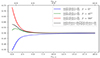Fig. 7. Ratio of the magnetic shifts produced by the prograde sectoral modes, ℓ = 2, m = −2 and ℓ = 1, m = −1, of the same radial order, n, as a function of their spin parameters, s1, −1 (lower x axis) and s2, −2 (upper x axis). The ratio was computed for three different angles of an inclined dipolar field, β = 0° (blue), β = 47° (green), and β = 90°. The ratio of the product, F(s)s3, which does not depend on the field topology, is also displayed (black).

We observe that the magnetic shift ratio, ω₁(2, −2, n)/ω₁(1, −1, n), is always smaller than one and that, for all inclination angles, it converges rapidly towards 1/2 as s increases. The asymptotic value of 1/2 is predicted by the asymptotic form of the magnetic shift of the two modes (see Eqs. (30) and (31)) and the asymptotic relation between the two spin parameters: s_2, −2 ≈ s_1, −1/2. The rapid convergence of ω₁(2, −2, n)/ω₁(1, −1, n) can be understood by looking at the weight functions of the two prograde sectoral modes computed, respectively, at s_1, −1 and s_2, −2. Figure 8 indeed shows that both functions become rapidly similar as s increases above one. This comes from the fact that at high s the prograde sectoral horizontal Hough functions behave as Gaussian functions whose widths are proportional to 1/( − ms)^1/2. Since s_2, −2 ≈ s_1, −1/2, the Gaussian widths of the two (ℓ = 2, m = −2, n) and (ℓ = 1, m = −1, n) Hough functions are very close, so that we expect and verify that the weight functions $K_{\theta }^{1,-1}(s_{1,-1})$ and $K_{\theta }^{2,-2}(s_{2,-2})$, and therefore the T_​​B factors of the two modes, are also very close. Crucially, this implies that the property, ω₁(2, −2, n)≈ω₁(1, −1, n)/2, holds for all field topologies but the rare ones that probe the small differences between the two latitudinal weight functions.

Fig. 8. Comparison of the latitudinal weight functions, Kθ, of the ℓ = 1, m = −1 (continuous lines) and ℓ = 2, m = −2 (dashed lines) modes of same radial order, n. The weight functions were computed for four (s1, −1, s2, −2) couples: (1.37, 0.71; black), (4.94, 2.47; blue), (9.5, 4.75; green), and (18.6, 9.3; red).

The ratio between the magnetic shifts of the r mode (k = −2, m = 1) mode and the prograde dipolar mode, ω₁(−2, 1, n)/ω₁(1, −1, n) is shown in Fig. 9. The s_1, −1 ∈ [0, 20] interval translates into s_−2, 1 ∈ [6, 20] for constant $s\sqrt{\mathrm{\Lambda }}$. As shown in Fig. 10, the weight function, K_θ, of the two modes are strongly concentrated towards the equator at high s. The ratio of the magnetic frequency shifts tends towards three in accordance with the analytical forms, Eqs. (30) and (32), and the asymptotic relation, s_−2, 1 ≈ 3s_−1, 1. We also observe that ω₁(−2, 1, n)/ω₁(1, −1, n) seems to diverge as s_−2, 1 approaches six. Indeed, at this point, $s_{1,-1}^3$ vanishes more rapidly than F_−2, 2, so that the ratio of s³F(s) terms goes to infinity. This s_1, −1 → 0 limit is however not relevant in practice because both magnetic shifts vanish and will thus be undetectable. It remains that, for s_1, −1 = 2, the ratio of the s³F(s) terms is equal to ∼7. For these low s_1, −1, the weight function profiles (see the blue curve in Fig. 10) also shows that the r mode is more sensitive to fields concentrated at the pole than the dipolar sectoral mode. This provides an opportunity to probe magnetic fields in both polar and equatorial regions.

Fig. 9. Ratio of the magnetic shifts of the r mode, k = −2, m = 1, and the prograde dipolar mode, ℓ = 1, m = −1, of the same radial order, n, as a function of their spin parameters, s1, −1 (lower x axis) and s−2, 1 (upper x axis). The ratio was computed for three different angles of an inclined dipolar field, β = 0° (blue), β = 47° (green), and β = 90° (red). The ratio of the product, F(s)s3, which does not depend on the field topology, is also displayed (black).

Fig. 10. Comparison of the latitudinal weight functions, Kθ, of the ℓ = 1, m = −1 (continuous lines) and k = −2, m = 1 (dashed lines) modes of same radial order, n. The weight functions were computed for three (s1, −1, s−2, 1) couples: (2.2, 8.9; blue), (9.5, 29.5; green), and (18.6, 56.8; red).

The ratio between the zonal and prograde dipolar mode magnetic shifts, ω₁(1, 0, n)/ω₁(1, −1, n), is shown in Fig. 11. The s_1, −1 ∈ [0, 20] interval translates into s_1, 0 ∈ [0, 4.5] for constant $s\sqrt{\mathrm{\Lambda }}$. The decrease in the ratio towards high s is close to 3/(2s_1, 0), in agreement with the analytical forms, Eqs. (30) and (33), and the asymptotic relation, $s_{1,0}=\sqrt{s_{1,-1}}$. For 1 ≲ s_1, 0 ≲ 2.5, the range of observed s_1, 0 in Li et al. (2020), the magnetic shift ratio is higher than one if β is low enough and is smaller than one for higher β. Consequently, depending on the field topology, the rotational splitting, ω₁(1, −1, n)−ω₁(1, 0, n), can be either larger or smaller than the unmagnetised TAR predictions. Such rotational splittings were determined by Li et al. (2020) for 11 stars and it was found that they can be either higher or smaller than the TAR prediction. Magnetic fields are thus a potential candidate to explain these observations. The weight functions of the two modes are shown in Fig. 12.

Fig. 11. Ratio of the magnetic shifts produced by the zonal dipolar mode, ℓ = 1, m = 0, and the prograde dipolar mode, ℓ = 1, m = −1, of the same radial order, n, as a function of their spin parameters, s1, −1 (lower x axis) and s1, 0 (upper x axis). The ratio was computed for three different angles of an inclined dipolar field, β = 0° (blue), β = 47° (green), and β = 90° (red). The ratio of the product, F(s)s3, which does not depend on the field topology, is also displayed (black).

Fig. 12. Comparison of the latitudinal weight functions, Kθ, of the ℓ = 1, m = −1 (continuous lines) and ℓ = 1, m = 0 (dashed lines) modes of same radial order, n. The weight functions were computed for four (s1, −1, s1, 0) couples: (1.37, 1.01; black), (4.94, 2.21; blue), (9.5, 3.08; green), and (18.6, 4.32; red).

3.2.2. Using both (ℓ,m) = (1, −1) and (ℓ,m) = (2, −2) frequency patterns to detect and measure the magnetic frequency shift

We now propose a method of searching for and measuring magnetic fields in stars where both (ℓ = 2, m = −2) and (ℓ = 1, m = −1) frequency patterns are present. If frequencies with the same radial order have been identified in these two frequency patterns, it is possible to compute the difference between the (ℓ = 1, m = −1, n) frequency and half the (ℓ = 2, m = −2, n) frequency, denoted δK (as it involves two Kelvin modes). If magnetic effects can be treated perturbatively, it reads

$$\begin{array}{cc}\hfill \delta K_{\mathrm{in}}& ={\nu }_{\mathrm{in}}(1,-1,n)-\frac{{\nu }_{\mathrm{in}}(2,-2,n)}{2}\hfill \\ \hfill & ={\nu }_0(1,-1,n)-\frac{{\nu }_0(2,-2,n)}{2}+{\nu }_1(1,-1,n)-\frac{{\nu }_1(2,-2,n)}{2}\hfill \end{array}$$(35)

$$\begin{array}{cc}\hfill & \approx {\nu }_0(1,-1,n)-\frac{{\nu }_0(2,-2,n)}{2}+\frac{3}{4}{\nu }_1(1,-1,n)\hfill \end{array}$$(36)

$$\begin{array}{cc}\hfill & \approx \frac{3}{4}{\nu }_1(1,-1,n).\hfill \end{array}$$(37)

The first approximated equation, Eq. (36), comes from the relation, ω₁(2, −2, n)≈ω₁(1, −1, n)/2, found in Sect. 3.2.1. Equation (36) then gives the magnetic shift, ν₁(1, −1, n), if the same difference between the unperturbed frequencies, $\delta K_0={\nu }_0(1,-1,n)-\frac{{\nu }_0(2,-2,n)}{2}$, can be determined. This can be done in principle using a seismic determination of Ω and an unmagnetised oscillation model. But, we also expect δK₀ to be small and, if it is negligible, compared to $\frac{3}{4}{\nu }_1(1,-1,n)$, then Eq. (37) holds, giving direct access to the magnetic frequency shift from the two observable frequencies, ν_in(1, −1, n) and ν_in(2, −2, n).

The difference, δK₀, should indeed be small because it vanishes for high-s, high-order TAR modes (as s_2, −2 = s_1, −1/2 in this limit). If we still assume high n TAR modes but now consider finite s, δK₀ is 9.6 nHz at s_1, −1 = 5 (for a rotation period of one day) and decreases for higher s_1, −1. We also determined δK₀ with more realistic frequencies computed from a stellar model and using the TOP code (Reese et al. 2006, 2009) to relax the TAR of the Coriolis force. The structure of this model has been computed with the CESAM evolution code (Morel 1997; Morel & Lebreton 2008). It has a mass, M = 1.4 M_⊙, a radius, R = 1.38 R_⊙, and a central hydrogen abundance, X_c = 0.68. The oscillation spectrum has been computed for a rotation, ν_rot = 1.28 d⁻¹. In Fig. 13, we show that δK₀ decreases from ∼20 nHz to ∼7 nHz between s_−1, 1 = 5 and s_−1, 1 = 7. This remains small although it is a bit higher than the same difference computed for high n TAR modes.

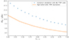Fig. 13. Small difference, δK0 = ν0(1, −1, n)−ν0(2, −2, n)/2, computed in the s1, −1 ∈ [5, 7] interval for two models: a high-order TAR model at νrot = 1.28 d−1 (orange line) and n ∈ [41, 56] modes computed with the TOP code for a M = 1.4 M⊙, R = 1.38 R⊙, Xc = 0.68 stellar model rotating at νrot = 1.28 d−1 (blue crosses).

While δK₀ tends to vanish as n increases, the magnetic shift, ν₁(1, −1, n), increases with n (or s), as described by Eq. (30). Thus, observing that δK_in ≈ δK₀ + 3ν₁(1, −1, n)/4 increases with n is already a clue of the presence of a magnetic field. Fitting δK_in with Eq. (30) then gives access to $B_{\text{eq}}^2$ and D_eq.

To test further the method proposed here, the properties of the difference δK₀ should be studied for various stellar models, including the effects of steep chemical gradients above the convective core, differential rotation, and centrifugal deformation. These effects are briefly discussed in Sect. 4.

3.3. Probing magnetic signatures in frequency spectra

In this section, we construct frequency spectra of prograde sectoral modes, (ℓ = 1, m = −1) and (ℓ = 2, m = −2), affected by a radial magnetic field in order to test simple methods of revealing magnetic signatures.

The spectra read ν_in = ν₀ − mν_rot + ν₁, where the index, “in”, indicates a frequency in the inertial frame, ν₀ is the unperturbed frequency in the co-rotating frame, and ν₁ is the magnetic frequency shift. The unperturbed frequency was computed using the TAR high-order approximation (Eq. (7)), with ${\mathrm{\Lambda }}_{m,-|m|}=m^2\frac{2ms}{2ms+1}$, ν_rot = 1 day⁻¹, and Π₀ = 4122 s, for radial orders n ∈ [35, 65]. The range of considered radial orders, the rotation frequency, ν_rot, and the spacing period, Π₀, correspond to typical values of the ∼700 (ℓ,m) = (1, −1) and (ℓ,m) = (2, −2) patterns identified by Li et al. (2020).

This specific period, Π₀ = 4122 s, has been calculated from a mid-main-sequence stellar model of a γ Dor star (M = 1.6 M_⊙, R = 2.13 R_⊙, X_c = 0.35), which we use in this section. It has been computed with the CESAM evolution code, by including turbulent diffusion of chemicals, D = 400 cm² s⁻¹. It possesses a convective core with a radius r_cc = 0.069R.

The magnetic frequency shifts, ${\nu }_1^{1,-1}$ and ${\nu }_1^{2,-2}$, were determined by Eqs. (30) and (31), assuming D_eq = 0 for simplicity. This stellar model and three different radial field profiles were considered to compute $\mathcal{I}{B}_{\mathrm{eq}}^2$ and then the magnetic frequency shifts. The first case (profile U) is a uniform field, B_r = 20 kG, between r_cc, the radius of the convective core, and r = 0.5R. For the two other profiles, we consider that B_r is 24.3 kG at r = r_cc and decreases exponentially by one order of magnitude either at r = 0.2R (profile B+) or at r = r_cc + 0.02R (profile B–). The magnetic frequency shifts, ${\nu }_1^{1,-1}$, computed for the frequency corresponding to s_1, −1 = 5 are 110, 37, and 9.1 nHz, for these three configurations, respectively. The magnetic frequency shift, ${\nu }_1^{2,-2}$, is simply ${\nu }_1^{1,-1}/2$ at s_2, −2 = s_1, −1/2.

These values are larger or just above the frequency resolution of Kepler for classical pulsators (1/T = 7.9 nHz for T = 4 yr). In practice, models are not able to fit observed frequencies at this level of accuracy so that the magnetic frequency shifts should rather be compared with other source of frequency deviations such as the differential rotation or the steep gradient of molecular weight overlying the convective core.

Figure 14 shows the observed period spacings, ΔP, of the (ℓ = 1, m = −1) modes as a function of the period, P, for the different magnetic cases. The ΔP − P diagrams are frequently used to determine the period, Π₀, and the rotation frequency, ν_rot, using the TAR (e.g. Van Reeth et al. 2015; Li et al. 2019). The magnetic field does not produce noticeable signatures on the shape of the profile of ΔP: it slightly changes its mean value and its slope. Such changes can be mimicked by a modification of Π₀ and/or ν_rot and may bias the determination of these parameters. To show this, we analysed the magnetically shifted frequency patterns with methods that do not take magnetic effects into account. We thus applied the method developed by Christophe et al. (2018) to the frequency sets of prograde dipolar and quadripolar modes generated with the magnetic field profiles U, B+, and B–. This method returns the period spacing, Π₀, and the rotation frequency, ν_rot, that best fit a frequency set within the TAR. Once Π₀ and ν_rot were determined, we identified the radial orders, n, of the modes and the offset, ϵ_g (see Eq. (7)). Table 1 summarises the results obtained for the different cases and Fig. 15 shows the difference between the simulated frequencies and the fitted frequencies. First, we notice that the fits are in good agreement and the residuals between input and fitted frequencies do not generally exceed a few nHz. It means that a model without a magnetic field can correctly reproduce data that are indeed affected by a magnetic field. However, the values of Π₀ and ν_rot are biased towards larger values. The stronger the magnetic shift is, the stronger the bias is: (ℓ = 1, m = −1) modes are more sensitive to magnetic field than (ℓ = 2, m = −2) modes and the effect are the largest for profile U and the smallest for profile B–. The presence of a magnetic field also lowers the apparent value of the offset, ϵ_g. This effect can be strong enough to not only modify ϵ_g, but also to shift the apparent values of the radial order, n (it is the case for the profile U and for ℓ = 1 with the profile B+, see Table 1).

Fig. 14. Period spacing, ΔP, of (ℓ = 1, m = −1) modes as a function of their periods for a model with a magnetic field following the radial profiles U (orange), B+ (red), and B– (green). The non-magnetic case is also shown (black).

Fig. 15. Residuals between simulated frequencies and the fitted frequencies obtained with the method of Christophe et al. (2018) applied to the simulated data set with the profiles U (orange), B+ (red), and B– (green). The left (resp., right) panel shows results for ℓ = 1 (resp., ℓ = 2) modes.

Considering a real star for which only (ℓ = 1, m = −1) modes are observed, biases of Π₀ and ν_rot can hardly be spotted since the real values of these quantities are a priori unknown. However, for strong fields (such as with profile U, or with profile B+ to a lesser extent) we may identify the existence of a magnetic effect by analysing the departure of the observed frequencies from the TAR prediction. This difference can be revealed in a stretched échelle diagram, in which mode frequencies are plotted as a function of the period in the corotating frame, stretched with the Λ function, modulo the period spacing, Π₀ (Fig. 16). Within the TAR, modes form vertical lines in stretched échelle diagrams. We see in Fig. 16 that a magnetic field distorts the ridge in a S-shape profile with an amplitude larger than 500 s (for profile U). This signature can be compared to various effects studied in Christophe et al. (2018), especially in their Fig. 5. First, we notice that the differences between complete computations and the TAR are clearly smaller (< 100 s). Second, buoyancy glitches generate oscillating signatures with amplitudes similar to the ones produced by a strong magnetic field, but their periodic nature helps to discriminate between both. Finally, a strong differential rotation also produces a smooth change in the ridge shape, but with a very small amplitude and mainly induces avoided crossings between modes, which create a quite different signature to the one shown in Fig. 16.

Fig. 16. Stretched échelle diagram from a magnetically shifted frequency spectra (profile U), obtained by applying the method of Christophe et al. (2018). Modes are plotted twice for clarity.

Having both (ℓ = 1, m = −1) and (ℓ = 2, m = −2) frequency patterns aids the detection of seismic magnetic signatures. Table 1 indeed shows clear differences in the values of Π₀ obtained for each pattern. For the U magnetic profile, the (ℓ = 1, m = −1) pattern provides a period spacing 21% larger than the (ℓ = 2, m = −2) pattern. This corresponds to a difference of 922 s, which is larger than most errors in the Π₀ determination quoted in Li et al. (2020). The difference in the ν_rot values is smaller, although the 0.05 d⁻¹ discrepancy is also larger than most errors in ν_rot values quoted in Li et al. (2020). For the weakest magnetic shifts (profile B–), the difference in Π₀ is at the level of the best-fitting errors indicated in Li et al. (2020).

The (ℓ = 1, m = −1) and (ℓ = 2, m = −2) frequency patterns can also be combined to detect and measure the magnetic frequency shifts. Using the radial order identifications provided by the fits (see Table 1), the difference, δK_in, introduced in Sect. 3.2.2 can be computed as a function, n. In a non-magnetic star, δK_in = δK₀ is small (of the order of 10 nHz) and a decreasing function of n, whereas a magnetic term increasing with n adds up in a magnetic star. As the order identifications may be wrong, differences formed by shifting the radial orders of one of the pattern ν_in(ℓ = 1, m = 1, n + n_s)−ν_in(ℓ = 2, m = 2, n)/2 were computed until the smallest positive difference was found. The result of this process is shown in Fig. 17 for the three magnetic profiles considered. We observe that the smallest positive difference is an increasing function of n for the three magnetic profiles. As explained in Sect. 3.2.2, this quantity is close to $3{\nu }_1^{1,-1}/4$ and can be used to derive the magnetic seismic observables, B_eq and D_eq. Here, δK₀ = 0 because we computed the unperturbed frequencies in the asymptotic regime. In real stars, the magnetic term will need to be higher than δK₀ for the smallest positive difference, ν_in(ℓ = 1, m = 1, n + n_s)−ν_in(ℓ = 2, m = 2, n)/2, to be an increasing function of n. Considering that δK₀ is of the order of 10 nHz as in the realistic model considered in Sect. 3.2.2 (see Fig. 13), a magnetic signature would be detected for the magnetic profiles U and B+.

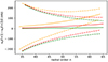Fig. 17. Magnetic shift computed from the difference, δKin for the magnetic profile U (orange), B+ (red), and B– (green), as a function of the apparent radial order, n, of ℓ = 2 modes. We notice that for the profile U, the apparent radial orders are shifted compared to the real ones (see Table 1 and text for a discussion). Dashed lines are obtained when the radial order of ℓ = 1 modes is incorrectly identified compared to the radial order of ℓ = 2 modes by ±1.

4. Summary and discussion

We used a perturbative method to investigate the frequency shift induced by an arbitrary magnetic field on gravito-inertial modes. From the general expression of the magnetic frequency shift, Eq. (10), we derived approximated simplified formulas valid for short radial wavelength gravito-inertial modes described by the TAR. This allowed us to determine the frequency dependence of the magnetic shift for the modes most often observed in γ Dor stars, the (ℓ,m) = (1, −1),(2, −2),(1, 0) g modes and the (k, m) = (−2, 1) r mode, and to define the seismic observable quantities and their relation with the internal magnetic field. We find that the magnetic frequency shift is larger for low-frequency modes and for strong equatorial radial fields. Comparing magnetic shifts of different modes with the same radial order, n, we find that the (k = −2, m = 1) r mode is the most sensitive to magnetic field followed by the (ℓ = 1, m = −1) g mode. We then proposed simple methods to detect magnetic signatures: the characteristic form of the error when the frequency pattern is analysed with a non-magnetic model, the discrepancy between the period spacings, Π₀, determined, respectively, with the (ℓ,m) = (1, −1) and the (ℓ,m) = (2, −2) frequency patterns analysed with a non-magnetic model, and the determination of the magnetic shift from the difference, δK_in = ν_in(1, −1, n)−ν_in(2, −2, n)/2.

Before starting the discussion of our results, we first have to mention a clear discrepancy between our results and those presented in Prat et al. (2019, 2020). The magnetic shifts computed in these papers result in a sawtooth pattern in the period spacing versus period relation. This feature is incompatible with the smooth variations of the magnetic shift with s (or n) that we find in both our numerical and analytical results. We notice that in Prat et al. (2019) the equations relating the horizontal Hough functions to the radial Hough function given in their Appendix A are not correct.

In the following, we first discuss the approximations made to derive the simplified formulas of the magnetic frequency shifts, then the conditions for applying the perturbative method, and finally the origin and detectability of magnetic fields in γ Dor radiative zones.

4.1. Approximations in the derivation of the magnetic shifts

In the regime of short radial wavelengths, the effect of the radial component of the magnetic field tends to dominate over the horizontal components. As already discussed in Li et al. (2022), the contribution of the horizontal components to the magnetic shift can be neglected if k_rB_r ≫ k_θB_θ and k_rB_r ≫ k_ϕB_ϕ, where (k_r, k_θ, k_ϕ) are the components of the mode wave vector. When applied to high-n, high-s TAR oscillations, these conditions translate into upper limits of the ratio of the horizontal to radial components, namely, B_ϕ/B_r ≪ (N/ω₀) and B_θ/B_r ≪ (N/2Ω)^1/2(N/ω₀)^1/2, (see details in Appendix A). For a (ℓ,m) = (1, −1) mode of spin parameter s = 5 in a M = 1.6 M_⊙, R = 2.13 R_⊙, X_c = 0.35, ν_rot = 1 d⁻¹ star model, these constraints are B_ϕ/B_r ≲ 125 and B_θ/B_r ≲ 55 near the bottom of the radiative zone. If the horizontal field contributions were not negligible, a different frequency dependence of the magnetic shift is expected and this property can be used to identify a situation where the radial field is not dominant. Indeed, as argued by Li et al. (2022) in the case of slowly rotating stars, the magnetic shift varies as ∝1/ω₀ for purely azimuthal fields, a frequency dependence that can be distinguished from the $\propto 1/{\omega }_0^3$ dependence produced by radial fields. The numerical results of Dhouib et al. (2022) obtained for a rapidly rotating star with azimuthal fields also indicate that the increase in the magnetic shift with decreasing ω₀ is much slower than $\sim 1/{\omega }_0^3$ (see their Fig. 11).

We also used the TAR to describe the effects of the star rotation on g modes. The TAR has been tested against two oscillation codes, TOP (Reese 2006; Reese et al. 2009) and ACOR (Ouazzani et al. 2012), which include a full treatment of the Coriolis and centrifugal accelerations. It was found the TAR generally provides a good approximation when the centrifugal deformation is not too strong (Ballot et al. 2012; Ouazzani et al. 2017) although it fails in some specific frequency intervals where the so-called Rosette modes (Ballot et al. 2012; Takata & Saio 2013) are observed or where gravito-inertial modes resonantly interact with convective core inertial modes (Ouazzani et al. 2020).

We recall that, when necessary, the approximations made to obtain simplified forms of the perturbative magnetic frequency shifts can be avoided by directly applying Eq. (10) to a chosen field configuration and to unperturbed modes computed for a particular stellar model with full oscillation codes like TOP or ACOR. It may then be necessary to use the full expression of the Lorentz term, ⟨ξ₀,ℒ_L(ξ₀)⟩, derived in Prat et al. (2020).

4.2. The limits of the perturbative methods

Another limit of the present study is that perturbative methods only apply when the strength of the magnetic field is low enough. The frequency deviation produced by the magnetic field must be small compared with the unperturbed frequency (i.e. ω₁ ≪ ω₀). For the synthetic spectra studied in Sect. 3.3, the magnetic shifts indeed remained much smaller than the unperturbed frequencies (the largest ratio is ω₁/ω₀ = 0.048 and corresponds to the strongest field and lowest frequency considered). Non-perturbative calculations are nevertheless necessary to determine the accuracy of the perturbative method. In a recent study, Rui et al. (2023) investigated the regime of strong non-perturbative magnetic fields in the particular case of a dipolar field aligned with the rotation rate. They show that perturbative methods can deviate significantly from the non-perturbative results when the field strength is close to the critical radial field above which gravity waves no longer propagate radially. As mentioned in the introduction, this critical radial field has been invoked to account for the unexpectedly low-amplitude, ℓ = 1 g modes observed in about 20% of red giants (Fuller et al. 2015). In our case, a critical radial field puts constraints on the possible amplitude of the magnetic shifts. Indeed, when a mode is observed, it means the internal radial magnetic field is everywhere smaller than the critical field, which in turn limits the amplitude of the magnetic frequency shift. For a full observed spectrum, the condition must hold for the smallest frequency because B_c ∝ ω². To construct the (ℓ,m) = (1, −1) frequency patterns of Sect. 3.3, we did choose radial fields such that B_r < B_c(ν_min). The exact value of B_c, which is the subject of ongoing research (Rui & Fuller 2023; Rui et al. 2023), should depend on the mode and the field geometries. Using $B_c=a\sqrt{4\pi \rho }(r/N){\omega }_0^2$ with a ≈ 1/2 as in Rui & Fuller (2023) for ℓ = 1, m = −1 modes, we find B_c = 24.3 kG at the bottom of the wave cavity near r = r_cc and B_c = 21.6 kG at r = 0.5R for the stellar model considered. Both constraints limit the amplitude of the magnetic shifts. Finally, we note that an upper limit of ν₁ = ν₀/(2a²) is obtained by assuming B_r = B_c(ν₀) everywhere in the wave cavity and using Eq. (30). But it is very unlikely to be reached as there is no physical reason for the actual stellar radial field to be equal to the field that prevents gravity wave propagation.

4.3. Origin and detectability of magnetic fields in γ Dor radiative zones

We now discuss the possible origin of magnetic fields in γ Dor radiative zones and whether they can produce detectable magnetic frequency shifts. Dynamo action generates magnetic fields in the convective core of γ Dors. Field strengths ranging between 10 and 100 kG are expected from numerical simulations of a 2 M_⊙ convective core by Brun et al. (2005) and equipartition fields determined using the mixing length theory (Cantiello et al. 2016). Numerical simulations also show that the dynamo field pervades the radiative layers just above the convective core, although its strength drops off sharply (Brun et al. 2005; Augustson et al. 2016). In Brun et al. (2005), the field intensity decreases by approximately one order of magnitude between r_cc and r_cc + 0.02R. A 100 kG radial field at r_cc with such a decrease into the overlying radiative layers produces magnetic shifts of ν₁ = 154 nHz for a (ℓ = 1, m = −1) frequency, corresponding to s = 5 and the stellar model M = 1.6 M_⊙, R = 2.13 R_⊙, X_c = 0.35 previously considered. However, this field exceeds the critical field, which is 24.3 kG at r = r_cc + 0.003R for the smallest frequency of a typical pattern, n ∈ [35, 65]. The fact that core dynamo fields can exceed the critical field for gravity wave propagation in γ Dor stars has already been put forward in Cantiello et al. (2016, see their Fig. 8 comparing B_c to a core dynamo field). These authors even suggest that this mode-suppression process explains why some stars in the γ Dors or SPB instability strips are not pulsating (see also Lecoanet et al. 2022). If instead we consider as in Sect. 3.3 a convective core field no larger than the critical field with the same exponential decrease, the magnetic shifts do not exceed ∼10 nHz. They would be very difficult if not impossible to detect even with Kepler data. However, the assumption of a sharp exponential decrease in the field strength does not take into account the decrease of convective core mass along the main sequence that leaves behind magnetic fields in radiative layers that were previously convective (Cantiello et al. 2016, see their Fig. 6). This process should increase the amplitude of the magnetic shifts in evolved γ Dors.

Other types of magnetic fields could be present in radiative interiors although we generally lack theoretical constraints on their strength and topology. This includes fossil magnetic fields possibly inherited from earlier evolutionary stages, either from the fully convective pre-main-sequence phase or from the stellar formation (Braithwaite & Spruit 2004; Lignières et al. 2014). Such fields could interact with the convective core as investigated by Featherstone et al. (2009). Moreover, in differentially rotating radiative zones, magnetic fields could be generated by dynamo processes triggered by the Tayler instability (Petitdemange et al. 2023) or the magneto-rotational instability (Guseva et al. 2017).

Spectroscopic observations provide constraints on surface fields. The Ap/Bp stars, a class of intermediate-mass main-sequence stars, are known to harbour surface fields with a typical value of 1 kG. The radial weight function plotted in Fig. 4 shows that envelope fields of such strength would produce a frequency shift of the same order as a 100-kG field at the bottom of the radiative zone. While interesting, this situation should remain unusual among γ Dors because the incidence of Ap/Bp stars is very low (less than 1%) in the mass range 1.4 M_⊙ < M < 1.8 M_⊙ (Sikora et al. 2019). It is more common to find Ap/Bp stars among SPB stars, the B star HD 43317 being an example of a star with strong surface field and g-mode oscillations (Lecoanet et al. 2022). Deep spectropolarimetric surveys also revealed that much weaker magnetic fields ∼1 G might be present at the surface of many intermediate-mass stars (Lignières et al. 2009; Blazère et al. 2016). The magnetic shift produced by such envelope fields would be very small though.

In Sect. 3.3, we proposed methods to detect magnetic signatures based on the analysis of magnetically shifted asymptotic spectra. While promising, these methods should be tested with more realistic unperturbed spectra, that is, non-asymptotic spectra that include the effects of chemical composition gradients, differential rotation, and centrifugal deformation. In particular, robust generic properties of the small difference, δK₀ = ν₀(1, −1, n)−ν₀(2, −2, n)/2, in non-magnetic stars would be useful to detect magnetic fields. We can already notice from the study by Miglio et al. (2008) that steep chemical composition gradients seem to have a very small influence on the relation between (ℓ = 1, n) and (ℓ = 2, n) frequencies in slowly rotating stars (see their Fig. 27). It is also known that a weak radial differential rotation has the same effect on all high-n (ℓ,m) modes (Van Reeth et al. 2018; Takata et al. 2020) so that it will not modify the difference. While latitudinal differential rotation has been taken into account in studying gravito-inertial propagating waves (e.g. Ogilvie & Lin 2004; Prat et al. 2018), the effect of a latitudinal differential rotation on the frequencies of gravito-inertial modes has not been determined yet. However, as the (ℓ,m) = (1, −1, n) and (2, −2, n) modes have very similar latitudinal eigenfunctions (see Fig. 8), we anticipate that the effects of a weak latitudinal differential rotation will be similar for the two modes. Strong radial or latitudinal differential rotation would have stronger effects (as shown in Christophe et al. 2018 and Takata et al. 2020, a strong radial differential rotation induces avoided crossings between modes that produce large and localised deviations in the frequency pattern) but they have not yet been detected in γ Dor stars. The methods we propose offer new possibilities to search for internal magnetic fields in existing Kepler or TESS data or in future observations, especially the PLATO mission (Rauer et al. 2014), which will observe γ Dor stars as benchmark stars.

Acknowledgments

We acknowledge support from the project BEAMING ANR-18-CE31-0001 of the French National Research Agency (ANR) and from the Centre National d’Etudes Spatiales (CNES).

References

Appendix A: Simplification of the magnetic frequency shift for low frequency ω₀/N ≪ 1 gravito-inertial modes

The expression of the magnetic shift can be significantly simplified for low frequency gravito-inertial modes. Such a simplification has been proposed by Hasan et al. (2005) for low-frequency g modes. Here, we determine the conditions under which it holds for gravito-inertial modes. First, in the low-frequency regime, the horizontal displacement, ξ_h, dominates the radial one, ξ_r. Indeed, from mass conservation, we have ξ_h/ξ_r ∼ k_r/k_h, where k_r and k_h are radial and horizontal wave vectors associated with the eigenfunction. From the WKB analysis of the radial eigenvalue problem we have $k_r=\frac{N}{{\omega }_0}\frac{\sqrt{\mathrm{\Lambda }}}{r}$. The azimuthal wavevector is estimated from the azimuthal number, m, by k_ϕ ∼ m/r, while the latitudinal wave vector, k_θ, can be estimated from the half-width of the Hough functions in the high-s regime, that is, k_θ ∼ (|m|s)^1/2/r when Λ ∼ m² and $k_{\theta }\sim {(\sqrt{\mathrm{\Lambda }}s)}^{1/2}/r$ when Λ ≠ m². It follows that k_r/k_θ ∼ (N/2Ω)^1/2(N/ω₀)^1/2 when Λ ∼ m², while k_r/k_θ ∼ (N/2Ω)^1/2(N/ω₀)^1/2 for the r mode and k_r/k_θ ∼ (N/ω₀) for the axisymmetric dipolar mode. From the same estimate, we find that the radial derivatives terms dominate (e.g. r∂_rξ_h ∼ rk_rξ_h ≫ ξ_h). Assuming in addition that the magnetic field varies over large scales, L, such that Lk_r ≫ 1, the terms involving B_r dominate over the B_ϕ terms if B_ϕ/B_r ≪ k_r/k_ϕ and B_θ/B_r ≪ k_r/k_θ. This translates into B_ϕ/B_r ≪ (N/ω₀) and B_θ/B_r ≪ (N/2Ω)^1/2(N/ω₀)^1/2 for the mode considered here. For a (ℓ,m) = (1, −1) mode such that s = 5 in one-day rotation period, M = 1.6 M_⊙, R = 2.13 R_⊙, X_c = 0.35 stellar model, the anisotropy constraints on the magnetic field near the bottom of the radiative zone read B_ϕ/B_r ≲ 125 and B_θ/B_r ≲ 55.

As in (Li et al. 2022), these assumptions allow us to simplify the Lorentz operator. After some algebra and neglecting a surface term by assuming that it is negligible with respect to the volume integral term, we get

$$\begin{array}{c}\hfill <{\mathit{\xi }}_0,{\mathcal{L}}_{\mathrm{L}}({\mathit{\xi }}_0)>=\frac{1}{{\mu }_0}{\displaystyle {\int }_V{{\mathit{B}}^{\mathbf{\prime }}}_0^{\ast }·{{\mathit{B}}^{\mathbf{\prime }}}_{0}dV,}\end{array}$$(A.1)

where B′₀ = ∇ ∧ (ξ₀ ∧ B) takes the simplified form

$$\begin{array}{c}\hfill {{\mathit{B}}^{\mathbf{\prime }}}_0=e^{i(m\varphi +{\omega }_{0}t)}\left(\begin{array}{c}0\\ \frac{1}{r}\frac{\partial }{\partial r}(r{\xi }_h(r)B_r)H_{\theta }\\ \frac{i}{r}\frac{\partial }{\partial r}(r{\xi }_h(r)B_r)H_{\varphi }\end{array}\right),\end{array}$$(A.2)

which leads to

$$\begin{array}{c}\hfill {{\mathit{B}}^{\mathbf{\prime }}}_0^{\ast }·{{\mathit{B}}^{\mathbf{\prime }}}_0=\frac{1}{r^2}{\left|\frac{\partial }{\partial r}\left(r{\xi }_h(r)\right)\right|}^2{B}_r^2(H_{\theta }^2+H_{\varphi }^2)\end{array}$$(A.3)

and

$$\begin{array}{c}\hfill <{\mathit{\xi }}_0,{\mathcal{L}}_1({\mathit{\xi }}_0)>={\displaystyle {\int }_{r_i}^{r_o}{\left|\frac{\partial }{\partial r}\left(r{\xi }_h\right)\right|}^2{\int }_0^{2\pi }{\int }_0^{\pi }\frac{B_r^2}{{\mu }_0}(H_{\theta }^2+H_{\varphi }^2)sin\theta d\theta d\varphi dr.}\end{array}$$(A.4)

From ${\mathit{\xi }}_0^{*}\cdot {\mathit{\xi }}_0={\xi }_r^2{H}_r^2+{\xi }_h^2(H_{\theta }^2+H_{\varphi }^2)$, we have

$$\begin{array}{c}\hfill <{\mathit{\xi }}_0,{\mathit{\xi }}_0>=2\pi {\displaystyle {\int }_{r_i}^{r_o}{\int }_0^{\pi }\rho r^2({\xi }_r^2{H}_r^2+{\xi }_h^2(H_{\theta }^2+H_{\varphi }^2))sin\theta d\theta dr,}\end{array}$$(A.5)

where the first term, ${\xi }_r^2{H}_r^2$, can be neglected for low-frequency gravito-inertial modes.

In the TAR approximation, the Coriolis term, 2iΩ ∧ ξ₀, simplifies into 2iΩ cos θ e_r ∧ ξ₀, from which we get

$$\begin{array}{c}\hfill <{\mathit{\xi }}_0,2i\mathbf{\Omega }\wedge {\mathit{\xi }}_0>=8\pi \mathrm{\Omega }{\displaystyle {\int }_{r_i}^{r_o}{\int }_0^{\pi }\rho r^2{\xi }_h^{2}dr{\int }_0^{\pi }{H}_{\theta }{H}_{\varphi }cos\theta sin\theta d\theta .}\end{array}$$(A.6)

References

- Augustson, K. C., Brun, A. S., & Toomre, J. 2016, ApJ, 829, 92 [Google Scholar]
- Aurière, M., Wade, G. A., Silvester, J., et al. 2007, A&A, 475, 1053 [NASA ADS] [CrossRef] [EDP Sciences] [Google Scholar]
- Ballot, J., Lignières, F., Prat, V., Reese, D. R., & Rieutord, M. 2012, in Progress in Solar/Stellar Physics with Helio- and Asteroseismology, eds. H. Shibahashi, M. Takata, & A. E. Lynas-Gray, ASP Conf. Ser., 462, 389 [NASA ADS] [Google Scholar]
- Bedding, T. R., Murphy, S. J., Colman, I. L., & Kurtz, D. W. 2015, in The Space Photometry Revolution, eds. R. A. García, & J. Ballot, EPJ Web Conf., 101, 01005 [NASA ADS] [Google Scholar]
- Blazère, A., Petit, P., Lignières, F., et al. 2016, A&A, 586, A97 [NASA ADS] [CrossRef] [EDP Sciences] [Google Scholar]
- Borucki, W. J., Koch, D., Basri, G., et al. 2010, Science, 327, 977 [Google Scholar]
- Braithwaite, J., & Spruit, H. C. 2004, Nature, 431, 819 [Google Scholar]
- Brun, A. S., Browning, M. K., & Toomre, J. 2005, ApJ, 629, 461 [Google Scholar]
- Bugnet, L., Prat, V., Mathis, S., et al. 2021, A&A, 650, A53 [NASA ADS] [CrossRef] [EDP Sciences] [Google Scholar]
- Cantiello, M., Fuller, J., & Bildsten, L. 2016, ApJ, 824, 14 [NASA ADS] [CrossRef] [Google Scholar]
- Ceillier, T., Eggenberger, P., García, R. A., & Mathis, S. 2013, A&A, 555, A54 [NASA ADS] [CrossRef] [EDP Sciences] [Google Scholar]
- Christophe, S., Ballot, J., Ouazzani, R. M., Antoci, V., & Salmon, S. J. A. J. 2018, A&A, 618, A47 [NASA ADS] [CrossRef] [EDP Sciences] [Google Scholar]
- Deheuvels, S., Li, G., Ballot, J., & Lignières, F. 2023, A&A, 670, L16 [NASA ADS] [CrossRef] [EDP Sciences] [Google Scholar]
- Dhouib, H., Mathis, S., Bugnet, L., Van Reeth, T., & Aerts, C. 2022, A&A, 661, A133 [NASA ADS] [CrossRef] [EDP Sciences] [Google Scholar]
- Donati, J., & Landstreet, J. D. 2009, ARA&A, 47, 333 [NASA ADS] [CrossRef] [Google Scholar]
- Eckart, C. 1960, in Hydrodynamics of Oceans and Atmospheres (Elsevier Science& Technology, A Pergamon Press book) [Google Scholar]
- Featherstone, N. A., Browning, M. K., Brun, A. S., & Toomre, J. 2009, ApJ, 705, 1000 [Google Scholar]
- Friedlander, S. 1987, Geophys. J., 89, 637 [NASA ADS] [CrossRef] [Google Scholar]
- Fuller, J., Cantiello, M., Stello, D., Garcia, R. A., & Bildsten, L. 2015, Science, 350, 423 [Google Scholar]
- Fuller, J., Piro, A. L., & Jermyn, A. S. 2019, MNRAS, 485, 3661 [NASA ADS] [Google Scholar]
- Garcia, S., Van Reeth, T., De Ridder, J., & Aerts, C. 2022, A&A, 668, A137 [NASA ADS] [CrossRef] [EDP Sciences] [Google Scholar]
- Gerkema, T., & Shrira, V. I. 2005, J. Fluid Mech., 529, 195 [Google Scholar]
- Gomes, P., & Lopes, I. 2020, MNRAS, 496, 620 [NASA ADS] [CrossRef] [Google Scholar]
- Gough, D. O., & McIntyre, M. E. 1998, Nature, 394, 755 [Google Scholar]
- Gough, D. O., & Thompson, M. J. 1990, MNRAS, 242, 25 [Google Scholar]
- Gouhier, B., Jouve, L., & Lignières, F. 2022, A&A, 661, A119 [NASA ADS] [CrossRef] [EDP Sciences] [Google Scholar]
- Guseva, A., Hollerbach, R., Willis, A. P., & Avila, M. 2017, Phys. Rev. Lett., 119, 164501 [NASA ADS] [CrossRef] [Google Scholar]
- Hasan, S. S., Zahn, J. P., & Christensen-Dalsgaard, J. 2005, A&A, 444, L29 [NASA ADS] [CrossRef] [EDP Sciences] [Google Scholar]
- Lecoanet, D., Vasil, G. M., Fuller, J., Cantiello, M., & Burns, K. J. 2017, MNRAS, 466, 2181 [Google Scholar]
- Lecoanet, D., Bowman, D. M., & Van Reeth, T. 2022, MNRAS, 512, L16 [NASA ADS] [CrossRef] [Google Scholar]
- Lee, U., & Saio, H. 1997, ApJ, 491, 839 [Google Scholar]
- Li, G., Van Reeth, T., Bedding, T. R., Murphy, S. J., & Antoci, V. 2019, MNRAS, 487, 782 [Google Scholar]
- Li, G., Van Reeth, T., Bedding, T. R., et al. 2020, MNRAS, 491, 3586 [Google Scholar]
- Li, G., Deheuvels, S., Ballot, J., & Lignières, F. 2022, Nature, 610, 43 [NASA ADS] [CrossRef] [Google Scholar]
- Li, G., Deheuvels, S., Li, T., Ballot, J., & Lignières, F. 2023, A&A, 680, A26 [NASA ADS] [CrossRef] [EDP Sciences] [Google Scholar]
- Lignières, F., Petit, P., Böhm, T., & Aurière, M. 2009, A&A, 500, L41 [CrossRef] [EDP Sciences] [Google Scholar]
- Lignières, F., Petit, P., Aurière, M., Wade, G. A., & Böhm, T. 2014, in Magnetic Fields throughout Stellar Evolution, IAU Symp., 302, 338 [Google Scholar]
- Loi, S. T. 2021, MNRAS, 504, 3711 [NASA ADS] [CrossRef] [Google Scholar]
- Marques, J. P., Goupil, M. J., Lebreton, Y., et al. 2013, A&A, 549, A74 [NASA ADS] [CrossRef] [EDP Sciences] [Google Scholar]
- Mathis, S., & Bugnet, L. 2023, A&A, 676, L9 [NASA ADS] [CrossRef] [EDP Sciences] [Google Scholar]
- Mathis, S., Bugnet, L., Prat, V., et al. 2021, A&A, 647, A122 [EDP Sciences] [Google Scholar]
- Miglio, A., Montalbán, J., Noels, A., & Eggenberger, P. 2008, MNRAS, 386, 1487 [Google Scholar]
- Morel, P. 1997, A&AS, 124, 597 [NASA ADS] [CrossRef] [EDP Sciences] [Google Scholar]
- Morel, P., & Lebreton, Y. 2008, Ap&SS, 316, 61 [Google Scholar]
- Mosser, B., Belkacem, K., Pinçon, C., et al. 2017, A&A, 598, A62 [NASA ADS] [CrossRef] [EDP Sciences] [Google Scholar]
- Ogilvie, G. I., & Lin, D. N. C. 2004, ApJ, 610, 477 [Google Scholar]
- Ouazzani, R. M., Dupret, M. A., & Reese, D. R. 2012, A&A, 547, A75 [NASA ADS] [CrossRef] [EDP Sciences] [Google Scholar]
- Ouazzani, R.-M., Salmon, S. J. A. J., Antoci, V., et al. 2017, MNRAS, 465, 2294 [Google Scholar]
- Ouazzani, R. M., Marques, J. P., Goupil, M. J., et al. 2019, A&A, 626, A121 [NASA ADS] [CrossRef] [EDP Sciences] [Google Scholar]
- Ouazzani, R. M., Lignières, F., Dupret, M. A., et al. 2020, A&A, 640, A49 [NASA ADS] [CrossRef] [EDP Sciences] [Google Scholar]
- Petitdemange, L., Marcotte, F., & Gissinger, C. 2023, Science, 379, 300 [NASA ADS] [CrossRef] [Google Scholar]
- Prat, V., Mathis, S., Augustson, K., et al. 2018, A&A, 615, A106 [NASA ADS] [CrossRef] [EDP Sciences] [Google Scholar]
- Prat, V., Mathis, S., Buysschaert, B., et al. 2019, A&A, 627, A64 [NASA ADS] [CrossRef] [EDP Sciences] [Google Scholar]
- Prat, V., Mathis, S., Neiner, C., et al. 2020, A&A, 636, A100 [NASA ADS] [CrossRef] [EDP Sciences] [Google Scholar]
- Rauer, H., Catala, C., Aerts, C., et al. 2014, Exp. Astron., 38, 249 [Google Scholar]
- Reese, D. 2006, Ph.D. Thesis, Université Toulouse III – Paul Sabatier, France [Google Scholar]
- Reese, D., Lignières, F., & Rieutord, M. 2006, A&A, 455, 621 [NASA ADS] [CrossRef] [EDP Sciences] [Google Scholar]
- Reese, D. R., MacGregor, K. B., Jackson, S., Skumanich, A., & Metcalfe, T. S. 2009, A&A, 506, 189 [NASA ADS] [CrossRef] [EDP Sciences] [Google Scholar]
- Ricker, G. R., Winn, J. N., Vanderspek, R., et al. 2015, J. Astron. Telesc. Instrum. Syst., 1, 014003 [Google Scholar]
- Rui, N. Z., & Fuller, J. 2023, MNRAS, 523, 582 [NASA ADS] [CrossRef] [Google Scholar]
- Rui, N. Z., Ong, J. M. J., & Mathis, S. 2023, MNRAS, 527, 6346 [CrossRef] [Google Scholar]
- Sikora, J., Wade, G. A., Power, J., & Neiner, C. 2019, MNRAS, 483, 2300 [NASA ADS] [CrossRef] [Google Scholar]
- Stello, D., Cantiello, M., Fuller, J., et al. 2016, Nature, 529, 364 [Google Scholar]
- Takata, M., & Saio, H. 2013, PASJ, 65, 68 [NASA ADS] [Google Scholar]
- Takata, M., Ouazzani, R. M., Saio, H., et al. 2020, A&A, 635, A106 [NASA ADS] [CrossRef] [EDP Sciences] [Google Scholar]
- Townsend, R. H. D. 2003, MNRAS, 340, 1020 [Google Scholar]
- Townsend, R. H. D. 2020, MNRAS, 497, 2670 [NASA ADS] [CrossRef] [Google Scholar]
- Unno, W., Osaki, Y., Ando, H., Saio, H., & Shibahashi, H. 1989, Nonradial Oscillations of Stars, 2nd ed. (Tokyo: University of Tokyo Press) [Google Scholar]
- Van Reeth, T., Tkachenko, A., Aerts, C., et al. 2015, ApJS, 218, 27 [Google Scholar]
- Van Reeth, T., Tkachenko, A., & Aerts, C. 2016, A&A, 593, A120 [NASA ADS] [CrossRef] [EDP Sciences] [Google Scholar]
- Van Reeth, T., Mombarg, J. S. G., Mathis, S., et al. 2018, A&A, 618, A24 [NASA ADS] [EDP Sciences] [Google Scholar]
- Wade, G. A., Neiner, C., Alecian, E., et al. 2016, MNRAS, 456, 2 [Google Scholar]
- Wang, H., Boyd, J. P., & Akmaev, R. A. 2016, GMD, 9, 1477 [NASA ADS] [Google Scholar]