© The Authors 2024

1. Introduction

The classic evolutionary picture of solar-like stars with stellar cores spinning up after the end of the core hydrogen burning on the main sequence has been proven to be, for the most part, incorrect. Indeed, measurements from Beck et al. (2012), Mosser et al. (2012), Deheuvels et al. (2012, 2014, 2015, 2017, 2020), Di Mauro et al. (2016), Triana et al. (2017), Gehan et al. (2018), Tayar et al. (2019) have indicated a relatively slow rotation rate in radiative interiors during advanced stages, which is incompatible with the predicted rotation rates from classical hydrodynamic stellar models (e.g., Eggenberger et al. 2012; Ceillier et al. 2013; Marques et al. 2013). Among the key candidates to improve stellar evolution models and efficiently reproduce observations are magnetic fields. When considering magnetohydrodynamic evolution involving the modified Tayler-Spruit dynamo formalisms (Tayler 1980; Spruit 1999, 2002; Mathis & Zahn 2005; Fuller et al. 2019; Eggenberger et al. 2022; Moyano et al. 2023; Petitdemange et al. 2023), the observed core and surface rotation rates can be reproduced simultaneously. In addition, stable fossil fields resulting from past convective dynamo action might be present inside the radiative core of red giants and may impact the angular momentum transport (e.g., Mestel 1987; Duez & Mathis 2010). Theoretical predictions for the effect of magnetic fields in red giant stars’ internal radiative zones on the frequencies of the oscillations have been developed during the past few years (Loi & Papaloizou 2020; Loi 2020, 2021; Gomes & Lopes 2020; Bugnet et al. 2021; Mathis et al. 2021; Li et al. 2022; Bugnet 2022; Mathis & Bugnet 2023), and they have led to the detection of several magnetized red giant cores by Li et al. (2022), Deheuvels et al. (2023), Li et al. (2023), Hatt et al. (2024). These observed magnetic fields have in common a strong radial component up to a few hundred kilogauss in amplitude in the vicinity of the hydrogen-burning shell (H-shell). This is incompatible with the current Tayler-Spruit formalisms generating strong toroidal components (Fuller et al. 2019). The observed magnetic fields must therefore have a different origin and could result from the stabilization of past dynamo fields (e.g., Mestel 1987; Braithwaite 2008; Duez & Mathis 2010; Bugnet et al. 2021).

Magnetic fields at the surface of white dwarfs and intermediate-mass main-sequence stars have been observed to be large scale (for instance in F stars Seach et al. 2020; Zwintz et al. 2020), with a dipolar poloidal field often dominating the spectropolarimetry results (e.g., Donati & Landstreet 2009). This geometry and associated strength are compatible with those of the radial magnetic field component detected in red giant cores (Li et al. 2022; Deheuvels et al. 2023; Li et al. 2023), and could therefore have resulted from the conservation of such a field in the radiative interior. However, not only dipolar but also quadrupolar and higher-order components are also very often detected (Maxted et al. 2000; Euchner et al. 2005, 2006; Beuermann et al. 2007; Landstreet et al. 2017), and one pole can present stronger fields than the other (hereafter called offset dipoles, e.g., Wickramasinghe & Ferrario 2000; Vennes et al. 2017; Hardy et al. 2023a,b; Hollands et al. 2023). This enhances the need for the characterization of the geometry of fields detected in red giants’ internal radiative zones, as they might also not be pure dipoles. Accessing the magnetic field geometry inside the radiative interior during the red giant branch is key to understanding the origin of magnetic fields in white dwarfs and to properly constraining the evolution of stars by including magnetic effects. Indeed, if the amplitude of the field controls how fast the angular momentum is redistributed, the geometry is key to constraining how much material is going to be redistributed in the radiative zone and therefore in the burning layers.

From the current measurements by Li et al. (2022), Deheuvels et al. (2023), Li et al. (2023), we have access to the average radial magnetic field amplitude near the H-shell (Li et al. 2022, Bhattacharya et al. 2024). However, given the observed signatures in the frequency pattern, it is currently impossible to confirm the complexity of the topology of the internal field (as it is done through spectropolarimetry for surface fields) for some of these stars, as the signature of the dipolar configuration on dipolar mixed modes is partially degenerate with higher-order magnetic field configurations (for instance with a field with a quadrupolar component, see Mathis & Bugnet 2023).

We aim to lift the observational degeneracy between the magnetic field configurations from the use of combined constraints from dipolar (ℓ = 1) and quadrupolar (ℓ = 2) oscillations. In Sect. 2, we present analytical and computational developments to link the observed magnetic frequency asymmetries to the magnetic topology. In Sect. 3, we investigate the detectability of various magnetic field configurations as observed at the surface of stars with a radiative envelope. We discuss the detectability of mixed dipolar and quadrupolar configurations from a combined study of ℓ = 1 and 2 oscillation frequencies as well as the detectability study for offset magnetic fields along the rotation axis in Sect. 4. Finally, we conclude on the future potential of magnetoasteroseismology to unveil complex magnetic field topologies.

2. Methods

2.1. Choice of the magnetic field configurations

Magnetic fields observed at the surface of stars with radiative envelopes often present a large-scale topology. While dipolar magnetic fields have been observed (e.g., Donati & Landstreet 2009), higher-order and more complex configurations have also been detected through spectropolarimetry. For instance, Kochukhov et al. (2022) observed a distorted dipolar topology at the surface of φ Draconis, with a large inclination relative to the rotation axis and an asymmetry between the two magnetic poles. Cool Ap stars are known to exhibit an even more complex magnetic field topology; for example, 49 Cam has significant octupolar contributions, including toroidal components (Silvester et al. 2017). We chose three magnetic field topologies characterized by stable magnetic fields in the radiative zone and with low angular degree magnetic field configurations to be detectable using asteroseismic observables (ℓ = 1 and ℓ = 2 modes). The three magnetic field configurations are presented in Fig. 1 and discussed below. We note that in panels (a)-(c) in Fig. 1, we have used black lines to denote the direction of the poloidal field component and red (blue) color shading to denote the positive (negative) toroidal field component.

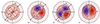Fig. 1. Schematics of plausible red giant magnetic topologies explored in this study. The left panel shows a schematic diagram showing a dipole and quadrupole (quadrudipole) magnetic field where the dipolar field component (solid black line) is inclined at an angle βd from the rotation axis and the quadrupolar component (dashed black line) is inclined at an angle βq from the rotation axis. The purple circle indicates the hydrogen burning shell. The inner light orange area indicates the radiative interior and the pink area indicates the convective envelope (not to scale). The three rightmost panels present the three magnetic field configurations used in our study as described in Sect. 3. Case (a) shows a quadrudipole magnetic field with aligned dipolar and quadrupolar axes, inclined with the rotation axis of an angle β = βd = βq. Case (b) shows an inclined mixed quadrudipole with βd the angle between the rotation axis and the dipolar field, and βq, the angle between the rotation axis and the quadrupolar field. Case (c) shows an offset dipole where the center of the dipole is shifted along the rotation axis by zo from the center of the star. For the three right panels, we have used red and blue shades to indicate the strength of the positive and negative toroidal field component. The black lines with arrows indicate field line directionality of the poloidal component.

Case (a) is a magnetic field with a dipolar component B_d and a quadrupolar component B_q (hereafter quadrudipole; see second panel of Fig. 1) that has aligned magnetic axes (β_d for the dipole is equal to β_q for the quadrupole, as defined in the left panel of Fig. 1). For this case, we allowed the magnetic field axis to be inclined in relation to the rotation axis with an angle β = β_d = β_q (aligned dipole and quadrupole), and we write the ratio of the magnetic field strength of the quadrupole over the dipole as ℛ. Hence,

$$\begin{array}{c}\hfill \mathit{B}(r,\theta ,\phi )={\mathit{B}}_d(r,\theta ,\phi )+\mathcal{R}{\mathit{B}}_q(r,\theta ,\phi ),\end{array}$$(1)

where (θ, φ) are the spherical coordinates with respect to the rotation axis and $(\stackrel{\sim }{\theta },\stackrel{\sim }{\phi })$ are the corresponding coordinates in a frame that is inclined at an angle β compared to the rotation axis.

Case (b) is a misaligned quadrudipole (see third panel of Fig. 1) where the dipolar and quadrupolar axes may have different inclination angles with respect to the rotation axis (β_d ≠ β_q):

$$\begin{array}{c}\hfill \mathit{B}(r,\theta ,\phi )={\mathit{B}}_d(r,{\theta }_d,{\phi }_d)+\mathcal{R}{\mathit{B}}_q(r,{\theta }_q,{\phi }_q),\end{array}$$(2)

where the coordinate system $({\stackrel{\sim }{\theta }}_d,{\stackrel{\sim }{\phi }}_d)$ is inclined by β_d with respect to the rotation axis and the coordinate system $({\stackrel{\sim }{\theta }}_q,{\stackrel{\sim }{\phi }}_q)$ is inclined by β_q with respect to the rotation axis. A recipe for constructing the rotated dipole and quadrupole is laid out in Appendix A for the readers’ convenience. We used simple identities offered by Wigner d-matrices for the necessary transformation between spherical coordinate systems.

Case (c) is an offset dipolar field with an offset along the rotation axis (see case (c) in Fig. 1), resulting in one pole being more magnetized than the other, as observed at the surface of white dwarfs (e.g., Wickramasinghe & Ferrario 2000):

$$\begin{array}{c}\hfill \mathit{B}(r,\theta ,\phi )={\mathit{B}}_d(\stackrel{\sim }{r}(z_o),\stackrel{\sim }{\theta }(z_o),\phi ),\end{array}$$(3)

where

$$\begin{array}{cc}\hfill \stackrel{\sim }{r}(z_o)& =\sqrt{r^2+z_o^2-2rcos\theta z_o},\hfill \end{array}$$(4)

$$\begin{array}{cc}\hfill \stackrel{\sim }{\theta }(z_o)& =\mathrm{atan}2(rsin\theta ,rcos\theta -z_o),\hfill \end{array}$$(5)

and z_o is the offset of the center of the field along the polar axis.

2.2. General definition of asymmetry parameters a_ℓ|m|

To investigate the detectability of these various large-scale magnetic field topologies inside the radiative interior of red giants, we used the asymmetry they induce on ℓ = 1 and ℓ = 2 mixed-mode frequencies (as demonstrated in Bugnet et al. 2021; Li et al. 2022). We considered a slowly rotating star to ensure that the rotation can be treated as a first-order perturbation (valid for slow rotators like red giants) and that this slowly rotating star is weakly magnetized following the derivation in Bugnet et al. (2021) (the magnetic field can as well be treated as a first-order perturbation). When carrying out a linearization of the magnetohydrodynamic equations about a magnetostatic background state, the Lorentz-state operator ℒ affecting oscillation frequencies may be expressed as (see Appendix A in Das et al. 2020, for further details)

$$\begin{array}{c}\hfill 4\pi \delta \mathcal{L}\mathit{\xi }={\mathbf{B}}_0\times (\mathbf{\nabla }\times {\mathbf{B}}_1)-(\mathbf{\nabla }\times {\mathbf{B}}_0)\times {\mathbf{B}}_1-\mathbf{\nabla }[\mathit{\xi }·({\mathbf{j}}_0\times {\mathbf{B}}_0)],\end{array}$$(6)

where B₀ and B₁ are the background and perturbed magnetic field, respectively; ξ is the eigenstate of the mode; and j₀ = ∇ × B₀ is the background current density.

For a high radial order g-dominated mixed mode, the coupling of eigenstate ξ_ℓ, m of a mode labelled by angular degree ℓ and azimuthal order m with eigenstate ξ_ℓ, m′ due to the magnetic linear operator ℒ is given by a magnetic coupling matrix M (Das et al. 2020; Li et al. 2022), such as

$$\begin{array}{c}\hfill {\mathbf{M}}_{\ell }{\mathbf{v}}_{\ell ,k}={\omega }_{\ell ,k}^1{\mathbf{v}}_{\ell ,k}\end{array}$$(7)

where ω_ℓ, k¹ are the 2ℓ+1 linearly perturbed eigenfrequencies corresponding to mode ℓ, v_ℓ, k are the corresponding eigenvectors, and the elements of the mode coupling matrix M_ℓ are defined as

$$\begin{array}{c}\hfill M_{\ell }^{m,m^{\prime }}=\frac{\langle {\mathit{\xi }}_{\ell ,m},\mathcal{L}\left({\mathit{\xi }}_{\ell ,m^{\prime }}\right)\rangle }{2{\omega }_{\ell }^0\langle {\mathit{\xi }}_{\ell ,m^{\prime }},{\mathit{\xi }}_{\ell ,m}\rangle },\end{array}$$(8)

where ω_ℓ⁰ is the unperturbed frequency of the mixed mode of order ℓ. As expressed in Li et al. (2022), and further supported by Bugnet et al. (2021) in the axisymmetric case, the magnetic field’s presence induces asymmetries in mixed mode multiplets. In our study, we consider that magnetic field effects are smaller than rotational effects, resulting in a M_ℓ matrix with dominant diagonal terms (we refer to Loi 2021, for the derivation of the full coupling matrix that includes effects of inclination of magnetic axis with respect to rotation axis). This is a reasonable assumption, as observed magnetic fields by Li et al. (2022), Deheuvels et al. (2023), Li et al. (2023) from ℓ = 1 frequencies are detected on multiplets containing 2ℓ+1 components, and not on (2ℓ+1)². Thus, by neglecting the off-diagonal terms, M_ℓ becomes a diagonal matrix, with the eigenfrequencies on the diagonal. In this case, k = m and we write (v_ℓ, m, ω_ℓ, m¹) instead. We generalized the formalism of Li et al. (2022) for the asymmetry induced by magnetic fields on ℓ = 1 mixed mode frequencies for any ℓ modes as

$$\begin{array}{c}\hfill {\delta }_{{\ell ,m}_{\mathrm{asym}}}={\omega }_{\ell ,-m}+{\omega }_{\ell ,m}-2{\omega }_{\ell ,0}=(2\ell +1)\zeta a_{\ell |m|}{\omega }_B^{\ell }.\end{array}$$(9)

In Eq. (9), ζ is the coupling function of the mixed modes (Goupil et al. 2013), and a_ℓ|m|, the asymmetry parameter, is defined as

$$\begin{array}{c}\hfill a_{\ell |m|}=\frac{M_{\ell }^{|m|,|m|}+M_{\ell }^{-|m|,-|m|}-2M_{\ell }^{0,0}}{\mathrm{Tr}\left({\mathbf{M}}_{\ell }\right)}\end{array}$$(10)

with $\mathrm{Tr}\left({\mathbf{M}}_{\ell }\right)={\displaystyle \sum _{m=-\ell }^{\ell }}{M}_{\ell }^{m,m}$, and ${\omega }_B^{\ell }$ the mean frequency shift:

$$\begin{array}{c}\hfill {\omega }_B^{\ell }=\frac{\mathrm{Tr}\left({\mathbf{M}}_{\ell }\right)}{2\ell +1}.\end{array}$$(11)

Figure 2 presents the definitions of the three asymmetry parameters used in our study, for ℓ = 1 (a₁₁) and ℓ = 2 (a₂₁, a₂₂) oscillations. In the following subsections we outline the two methods we have used to calculate magnetic frequency splittings (and hence asymmetry parameters) – (i) the analytical approach, similar to Mathis & Bugnet (2023), which adheres to the simplifying assumptions mentioned in the supplementary Sect. S2.2 of Li et al. (2022) and is sensitive to only the (θ, φ) angular dependence of B_r² and (ii) the numerical approach using magsplitpy (a rigorous computational framework for computing magnetic splittings due to a general magnetic field, following the theoretical underpinnings of Das et al. 2020), which is sensitive to all components of magnetic fields and provides the full solution.

Fig. 2. Definition of the asymmetry parameters aℓ|m| for the ℓ = 1 (top, as in Li et al. 2022) and ℓ = 2 (bottom) oscillation multiplets.

2.3. Analytical approach: Probing B_r

For a magnetic field B = (B_r, B_θ, B_φ), it is known that the dominant contribution to observed g-dominated mixed-mode frequency splitting comes from the B_r² component (Bugnet et al. 2021; Mathis et al. 2021) in the vicinity of the H-shell (Li et al. 2022; Bhattacharya et al. 2024). As shown in Eq. (30) of Li et al. (2022), the elements of this coupling matrix when considering only the dominant magnetic term can be approximated as

$$\begin{array}{cc}\hfill M_{\ell }^{m,m^{\prime }}& =\frac{1}{{\mu }_0}{\displaystyle {\int }_{r_i}^{r_o}}{\left[\frac{\partial (r{\xi }_h)}{\partial r}\right]}^2{\displaystyle {\int }_0^{2\pi }}{\displaystyle {\int }_0^{\pi }}{B}_r^2{e}^{i(m^{\prime }-m)\phi }\hfill \\ \hfill & \times [\frac{\partial {\widehat{Y}}_{\ell m}}{\partial \theta }\frac{\partial {\widehat{Y}}_{\ell m^{\prime }}}{\partial \theta }+\frac{m{m}^{\prime }}{{sin}^2\theta }{\widehat{Y}}_{\ell m}{\widehat{Y}}_{\ell m^{\prime }}]sin\theta \mathrm{d}r\mathrm{d}\theta \mathrm{d}\phi ,\hfill \end{array}$$(12)

where ξ_h is the radial variation of the horizontal component of the eigenfunction, $Y_{\ell m}(\theta ,\phi )={\widehat{Y}}_{\ell m}(\theta )e^{im\phi }$ and r_i, r_o, are the inner and outer turning points of the g-mode cavity. Using this analytical expression and the Racah-Wigner algebra derived in Appendix B of Mathis & Bugnet (2023), we obtain expressions for the various M_ℓ^m, m′ (see Mathis & Bugnet (2023) for ℓ = 1 modes, and our Appendix C for ℓ = 2 modes). From this, we obtain analytical expressions of the asymmetry parameters for various radial magnetic field topologies in Sect. 3.

For completeness, we also provide the analytical expressions for the configuration-independent form of the asymmetry parameters constructed from these matrix elements:

$$\begin{array}{cc}\hfill a_{21}& =\frac{{\displaystyle {\int }_{r_i}^{r_o}}K(r)\int \int B_r^2[8P_4(cos\theta )-P_2(cos\theta )]sin\theta \mathrm{d}\theta \mathrm{d}\varphi \mathrm{d}r}{7{\displaystyle {\int }_{r_i}^{r_o}}K(r)\int \int B_r^{2}sin\theta \mathrm{d}\theta \mathrm{d}\varphi \mathrm{d}r}\hfill \end{array}$$(13)

$$\begin{array}{cc}\hfill a_{22}& =\frac{4{\displaystyle {\int }_{r_i}^{r_o}}K(r)\int \int B_r^2[P_4(cos\theta )-P_2(cos\theta )]sin\theta \mathrm{d}\theta \mathrm{d}\varphi \mathrm{d}r}{7{\displaystyle {\int }_{r_i}^{r_o}}K(r)\int \int B_r^{2}sin\theta \mathrm{d}\theta \mathrm{d}\varphi \mathrm{d}r}\hfill \end{array}$$(14)

where, $K(r)={\left(\frac{\partial (r{\xi }_h)}{\partial r}\right)}^2$. This also provides consistency in the field where Li et al. (2022) provided these expressions for a₁₁, which we extend to a₂₁ and a₂₂.

2.3.1. A simple radial quadrudipole for theoretical calculations

Appendix A outlines the steps to obtain a rotation of a field on the surface of a sphere – going from being axisymmetric on the original coordinate system (θ, φ) to being non-axisymmetric on (θ, φ). As shown, we use identities of Wigner-d matrices to do so. In our case, we use the same analytical steps to tilt the axis of a dipolar and quadrupolar field by β_d and β_q respectively to obtain the expression for a general quadrudipole where the dipole and quadrupole are not necessarily axis-aligned. By simplifying the Wigner-d matrices required to tilt the field, we obtained the following analytical expression, which expands on the co-aligned case from Mathis & Bugnet (2023):

$$\begin{array}{cc}\hfill B_r(r,\theta ,\phi ,& \mathcal{R},{\beta }_d,{\beta }_q)=B_0{b}_r(r)\frac{1}{2}\sqrt{\frac{3}{\pi }}\hfill \\ \hfill & [cos{\beta }_{d}cos\theta +sin{\beta }_{d}sin\theta cos\phi \hfill \\ \hfill & +\frac{\sqrt{15}}{4}\mathcal{R}(\frac{1}{3}-{cos}^2{\beta }_q-{cos}^2\theta +3{cos}^2{\beta }_q{cos}^2\theta \hfill \\ \hfill & +sin2{\beta }_{q}sin2\theta cos\phi +{sin}^2{\beta }_q{sin}^2\theta cos2\phi )],\hfill \end{array}$$(15)

where ℛ is the ratio of the strength of quadrupole to dipole as defined in Mathis & Bugnet (2023). Here, we explicitly assume that both the dipole and the quadrupole have the same radial dependence b_r(r). This is a reasonable assumption since the dominating contribution from the magnetic field on the mode splitting occurs in the vicinity of the H-shell (Li et al. 2022; Bhattacharya et al. 2024); hence, the radial profile of the field does not significantly affect the magnetic field signature. We use this formalism in Sect. 3 to compute asymmetry parameters related to B_r² associated with various magnetic field topologies trapped in the radiative interior of the star. For an aligned quadrudipole (Case (a), such that β = β_d = β_q), this reduces to Eq. (25) and Eq. (28) of Mathis & Bugnet (2023) for ℛ = 0 and β = 0, respectively.

2.4. magsplitpy: Implementation of the full system

To estimate the signature of magnetic field topologies that are more complex than a quadrudipole, deriving an analytical expression is no longer efficient. In the same spirit as the inversion of rotation rates inside red giant stars from mixed-mode splitting (e.g., Deheuvels et al. 2012; Di Mauro et al. 2016; Ahlborn et al. 2020; Pijpers et al. 2021), Das et al. (2020) propose sensitivity kernels to probe a general magnetic field topology.

Das et al. (2020) formulated a prescription to infer the global solar magnetic field by using tools prevalent in terrestrial seismology (Dahlen & Tromp 1999). The Das et al. (2020) formalism is general enough to be seamlessly applied to other stars whose internal structure (and hence mode eigenfunctions) can be calculated from stellar evolution codes. In our study, we model a typical red giant star using MESA (Paxton et al. 2011, 2013, 2015, 2018, 2019; Jermyn et al. 2023) and compute its eigenfunctions and eigenfrequencies using GYRE (Townsend & Teitler 2013; Townsend et al. 2014). The MESA¹ computation is initialized with a mass of 1.5 M_⊙ and metallicity of Z = 0.02. We extracted the model for which Δν = 14.49 μHz, which represents a typical red giant branch star. We define R_h as the radius where the pp-nuclear reaction reaches its maximum, while R_c is the radius at which the Brunt-Väisälä frequency first goes to zero.

We note that Eqs. (13) and (14) for asymmetry parameters are linear combinations of Legendre polynomials, unlike just P₂(cosθ) as for a₁₁ as shown in Eq. (49) of Li et al. (2022). Consequently, going to higher angular degree modes comes with the asymmetry parameters being sensitive to more complex geometry. This is where the framework of magsplitpy becomes a powerful tool that we can use to numerically compute splittings or asymmetries for any general field topology. In a nutshell, magsplitpy would numerically evaluate matrix elements M_ℓ^m, m′ and using Eq. (10), we can then find the asymmetry parameters numerically. This is laid out in Sect. 2.4. Although in this study we primarily focus on the g-dominated core-sensitive modes of a typical red giant star, the magsplitpy framework can be used for g-dominated, p-dominated or highly mixed modes for core, intermediate or surface field detections.

2.4.1. Magnetic inversion kernels

Since the Lorentz force is given by (∇ × B)×B, the perturbation of interest are the components of the second rank Lorentz-stress tensor ℋ = BB. Therefore, to decompose these tensors in a spherical geometry, Das et al. (2020) used generalized spherical harmonics (GSH as in Appendix C of Dahlen & Tromp 1999) $Y_{\mathit{st}}^{\mu }(\theta ,\phi )$ such as

$$\begin{array}{cc}\hfill \mathbf{B}(r,\theta ,\phi )& ={\displaystyle \sum _{s=0}^{\infty }}{\displaystyle \sum _{t=-s}^s}{\displaystyle \sum _{\mu }}{B}_{\mathit{st}}^{\mu }(r)Y_{\mathit{st}}^{\mu }(\theta ,\phi ){\widehat{\mathit{e}}}_{\mu },\hfill \end{array}$$(16)

$$\begin{array}{cc}\hfill \mathcal{H}(r,\theta ,\phi )& ={\displaystyle \sum _{s=0}^{\infty }}{\displaystyle \sum _{t=-s}^s}{\displaystyle \sum _{\mu \nu }}{h}_{\mathit{st}}^{\mu \nu }(r)Y_{\mathit{st}}^{\mu +\nu }(\theta ,\phi ){\widehat{\mathit{e}}}_{\mu }{\widehat{\mathit{e}}}_{\nu },\hfill \end{array}$$(17)

where (μ, ν)∈{−1, 0, +1}² and the s and t subscripts denote the spherical harmonic angular degree and azimuthal order. We note that in this study, we used ℓ, m for mode harmonics and s, t for perturbation harmonics. The basis vectors in spherical polar coordinates can be transformed to those in the GSH basis using the following transformation:

$$\begin{array}{c}\hfill {\widehat{\mathit{e}}}_{-}=\frac{1}{\sqrt{2}}({\widehat{\mathit{e}}}_{\theta }-i{\widehat{\mathit{e}}}_{\phi }),{\widehat{\mathit{e}}}_0={\widehat{\mathit{e}}}_r,{\widehat{\mathit{e}}}_{+}=-\frac{1}{\sqrt{2}}({\widehat{\mathit{e}}}_{\theta }+i{\widehat{\mathit{e}}}_{\phi }).\end{array}$$(18)

for brevity of subscripts (and in keeping with the convention of Dahlen & Tromp 1999), we denote μ = −1, +1 in the subscripts as ${\widehat{\mathit{e}}}_{-},{\widehat{\mathit{e}}}_{+}$ respectively.

As a result, the general elements of the matrix M_ℓ are written as

$$\begin{array}{cc}\hfill M_{\ell }^{m,m^{\prime }}& ={\displaystyle \sum _{\mathit{st}}}{\displaystyle \sum _{\mu \nu }}{\displaystyle {\int }_0^{R_{\odot }}}\mathrm{d}r{r}_{m{m}^{\prime }}^2{\mathcal{B}}_{\mathit{st}}^{\mu \nu }(r)h_{\mathit{st}}^{\mu \nu }(r),\hfill \end{array}$$(19)

with $h_{\mathit{st}}^{\mu \nu }$ as the Lorentz-stress tensors for components (μ, ν) and the spherical harmonic as (s, t), while ${}_{mm\prime }{\mathcal{B}}_{\mathit{st}}^{\mu \nu }$ represents the respective magnetic inversion kernels. The complete expressions of the kernel components ${}_{mm\prime }{\mathcal{B}}_{\mathit{st}}^{\mu \nu }$ is laid out in Appendix B (presented for ease of readers’ reference but originally found in Das et al. 2020). A similar expression was derived in Mathis & Bugnet (2023). We note that since we are confined to the self-coupling of multiplets (same n, ℓ coupling), we suppressed these indices in the above expression.

2.4.2. Sensitivity of modes with degree ℓ to the magnetic field topology

To ask the question of which components of the magnetic field B are sensitive modes of degree ℓ, we need to see how the Lorentz-stress GSH is connected to the magnetic field GSH. This is because modes are sensitive to components of ℋ. As shown in Appendix D of Das et al. (2020), they are related as follows:

$$\begin{array}{cc}\hfill h_{\mathit{st}}^{\mu \nu }& ={\displaystyle \sum _{s_1,s_2,t_1,t_2}}{B}_{s_1{t}_1}^{\mu }{B}_{s_2{t}_2}^{\nu }\int Y_{\mathit{st}}^{\ast \mu +\nu }{Y}_{s_1{t}_1}^{\mu }{Y}_{s_2{t}_2}^{\nu }\mathrm{d}\mathrm{\Omega }\hfill \\ \hfill & ={\displaystyle \sum _{s_1,s_2,t_1,t_2}}{B}_{s_1{t}_1}^{\mu }{B}_{s_2{t}_2}^{\nu }{(-1)}^{\mu +\nu +t}\sqrt{\frac{(2s+1)(2s_1+1)(2s_2+1)}{4\pi }}\hfill \\ \hfill & \times \left(\begin{array}{ccc}{s}_1& s& \hfill s_2\\ \mu & -(\mu +\nu )& \hfill \nu \end{array}\right)\left(\begin{array}{ccc}{s}_1& s& \hfill s_2\\ t_1& -t& \hfill t_2\end{array}\right).\hfill \end{array}$$(20)

Whether or not a degree of perturbation s will induce a frequency splitting, depends on the angular degree ℓ of the mode of interest. This is controlled by the triangle rule imposed by the Wigner 3-j symbols in Eq. (20). For simplicity, we assume that the magnetic field is a pure dipole, that is, s₁ = s₂ = 1. By the Wigner 3-j triangle rule |s₁ − s₂|≤s ≤ s₁ + s₂, there would be only three degrees of Lorentz-stress tensor s = 0, 1, 2. When using self-coupling of ℓ = 1 modes, the odd degree s = 1 is insensitive since the kernel ${}_{\ell \ell }{\mathcal{G}}_1^{00}=0$ (we note that 𝒢 are the m independent forms of the full kernels ℬ, see Appendix B). So, for self-coupling, ℓ = 1 modes are only sensitive to s = 0, 2 components of Lorentz-stress. The magnetic field component s₁ = 1 contributes to both these Lorentz-stress components. Therefore, when using dipole modes ℓ = 1 (resp. quadrupole modes ℓ = 2), the splittings and asymmetry parameters are sensitive to only up to s = 2 (resp. s = 4) components of the Lorentz-stress tensor.

Therefore, the important conclusion from the above thought experiment is that we can only infer even components of the Lorentz stress. However, each of these components, let’s say s = 2, contains contributions from all magnetic field components s/2  ≤  s₁  ≤  ∞. So, the s = 0 Lorentz-stress has information from all B_r components with angular degree s₁ ≥ 0 (in reality s₁ ≥ 1, since s = 0 is a magnetic monopole). Similarly, the s = 2 Lorentz stress component has information from all B_r components with angular degree s₁ ≥ 1, the s = 4 Lorentz stress component has information from all B_r components with angular degree s₁ ≥ 2, and so on and so forth. Quadrupolar modes (ℓ = 2) are therefore extremely valuable for the search of complex magnetic field topologies, as ℓ = 2 oscillation mode frequencies are independent of the dipolar component of the magnetic field, and give a direct insight into the high-order of complexity of the field. This is the foundation of this study and justifies the need for ℓ = 2 mode characterization in the following sections.

2.4.3. Realistic quadrudipole configurations for signatures of the full magnetic field with magsplitpy

In order not only to check the theoretical results obtained from the simplified radial component of a quadrudipole but also to investigate the signature of more complex topologies in Sect. 3, we use a full quadrudipole topology in magsplitpy. Deriving a force-free stable quadrudipole magnetic field in the radiative interior from Broderick & Narayan (2008):

$$\begin{array}{cc}\hfill {\mathit{B}}_d(r,\theta ,\phi )& =C_d[\frac{j_1({\alpha }_{d}r)}{r}cos\theta {\widehat{\mathit{e}}}_r\hfill \\ \hfill & -\frac{{\alpha }_{d}r{j}_0({\alpha }_{d}r)-j_1({\alpha }_{d}r)}{2r}sin\theta {\widehat{\mathit{e}}}_{\theta }\hfill \\ \hfill & +\frac{{\alpha }_d{j}_1({\alpha }_{d}r)}{2}sin\theta {\widehat{\mathit{e}}}_{\phi }],\hfill \end{array}$$(21)

and

$$\begin{array}{cc}\hfill {\mathit{B}}_q(r,\theta ,\phi )& =C_q[\frac{j_2({\alpha }_{q}r)}{6r}(3{cos}^2\theta -1){\widehat{\mathit{e}}}_r\hfill \\ \hfill & -\frac{{\alpha }_{q}r{j}_1({\alpha }_{q}r)-2j_2({\alpha }_{q}r)}{6r}cos\theta sin\theta {\widehat{\mathit{e}}}_{\theta }\hfill \\ \hfill & +\frac{{\alpha }_q{j}_2({\alpha }_{q}r)}{6}cos\theta sin\theta {\widehat{\mathit{e}}}_{\phi }],\hfill \end{array}$$(22)

where j_{l ∈ [1, 2]} are the spherical bessel function of the first kind. The parameters α_d and α_q are chosen such that the conditions at the convective/radiative boundary are B_r(R_c) = B_φ(R_c) = 0 with R_c the radius of the radiative interior (see Prat et al. 2019; Bugnet et al. 2021, for more details about the method). As a result, both the quadrupolar and the dipolar field are zero outside the radiative region, that is, B(r ≥ R_c) = 0. Both fields are normalized such that B_r(R_h) = 1, where R_h is the radius of the H-shell in the radiative zone. Therefore, for the full numerical calculations using magsplitpy, we used the following 3D field:

$$\begin{array}{c}\hfill \mathit{B}(r,\theta ,\phi )={\mathit{B}}_d(r,\theta ,\phi )+\mathcal{R}{\mathit{B}}_q(r,\theta ,\phi ).\end{array}$$(23)

In this general field configuration, we define ℛ as the relative strength between radial components of the dipole and quadrupole at the H-shell. This is a reasonable choice because as evaluated in Bhattacharya et al. (2024) (and supported by Li et al. 2022), the hydrogen burning region represents about 90% of the sensitivity of the ℓ = 1, 2 oscillation modes in the core for the typical model red giant star chosen in our study and the radial component dominates the magnetic sensitivity over all other components. This quadrudipole general formalism is used in Sect. 3 to estimate the detectability of Cases (a), (b), and (c) from ℓ = 1 and ℓ = 2 oscillation asymmetries with magsplitpy.

3. Asymmetry parameters as a probe of magnetic field topologies

3.1. Aligned dipolar field and quadrupolar field axes

We first explore the simpler Case (a) of an aligned dipole and quadrupole defined in Eq. (1), that is, β_d = β_q = β, as previously done for ℓ = 1 oscillation modes in Mathis & Bugnet (2023). This reduces the parameters describing the topologies from the previous section to (ℛ,  β).

3.1.1. Analytical results from the asymmetry parameters associated with the radial component of the field

Plugging in the analytical definition of B_r from Eq. (15) into the simplified analytic expression in Eq. (12) and the definition of asymmetry parameter in Eq. (10), we obtained

$$\begin{array}{c}\hfill a_{11}=\frac{(7+5{\mathcal{R}}^2)(1+3cos2\beta )}{70(1+{\mathcal{R}}^2)}\end{array}$$(24)

for ℓ = 1 modes as in Mathis & Bugnet (2023) and

$$\begin{array}{cc}\hfill a_{21}& =\frac{-2+5{\mathcal{R}}^2+2(-3+5{\mathcal{R}}^2)cos2\beta +25{\mathcal{R}}^{2}cos4\beta }{140(1+{\mathcal{R}}^2)},\hfill \end{array}$$(25)

$$\begin{array}{cc}\hfill a_{22}& =-\frac{16+5{\mathcal{R}}^2+4(12+5{\mathcal{R}}^2)cos2\beta -25{\mathcal{R}}^{2}cos4\beta }{280(1+{\mathcal{R}}^2)}\hfill \end{array}$$(26)

for ℓ = 2 modes. Our study only considers β ∈ [0° :90° ] for all three a_ℓ|m| because of the symmetry relation

$$\begin{array}{c}\hfill a_{\ell |m|}(\mathcal{R},{90}^{°}-\beta )=a_{\ell |m|}(\mathcal{R},{90}^{°}+\beta ).\end{array}$$(27)

The first column of Fig. 3 represents the value of the a_ℓ|m| parameters as function of β and ℛ, from Eqs. (24), (25) and (26), where only the radial component of the magnetic field is used. The three rows in Fig. 3 show a₁₁, a₂₁ and a₂₂ (from top to bottom), respectively. Contour maps in these left panels of Fig. 3 can be used to show that there are no theoretical degeneracies between the quadrudipole and a pure dipole when using all three asymmetry parameters simultaneously. We see that if, from observations, we get a₁₁ > 0, a₂₁ > 0 and a₂₂ < 0, our possibility of configurations is limited to a strong quadrupole with a low inclination with respect to the rotation axis. A similar visual analysis of Fig. 3 shows how the availability of these three asymmetry parameters drastically reduces the possibilities in magnetic configurations. We conclude that the degeneracy of the quadrudipole with a pure dipolar field observed in Mathis & Bugnet (2023) is lifted when accessing ℓ = 1 and ℓ = 2 oscillation frequencies simultaneously. We discuss this in detail in Sect. 4.1.

Fig. 3. Color maps for each asymmetry parameter (top: a11, middle: a21, bottom: a22) for a co-aligned quadrudipole (βd = βq = β). The solid (dashed) overplotted contours emphasize the values of the asymmetry parameters. Only |ℛ| are shown since aℓ|m| are functions of ℛ2. There is a symmetry relation of aℓ|m|(90° −β) = aℓ|m|(90° +β) intrinsic to Eqs. (24)–(26); therefore, we limited β to the interval [0° ,90° ]. Left panels: ℓ = 1, 2 theoretical degeneracy for a magnetic field of the case (a) in Fig. 1. Middle panels: same degeneracy computed with magsplitpy. Right panels: Absolute difference between the numerical calculations and the analytical expressions of the asymmetry parameters.

We would also like to point out some salient features of the aligned quadrudipole: (i) For a₁₁, we recover the null line in asymmetry at ∼54.7° consistent with the findings in Mathis & Bugnet (2023). For all magnetic obliquity below this angle, a₁₁ is positive and vice-versa. For a given β, the strength of the asymmetry increases for a stronger dipolar component (smaller |ℛ|), (ii) For a pure dipole (or a small quadrupolar component) a₂₁ goes from being positive for high magnetic inclination to negative for intermediate and low inclinations. This changes to a double positive lobe at low and high β and a negative dip in intermediate β for stronger quadrupolar contribution. (iii) For a₂₂ we once, again have a more two-sided polarity where for low β the asymmetry is negative and vice-versa. The null line has a qualitatively different trend than a₁₁. Further, for very low inclinations and very strong quadrupolar contribution, we also have a near zero a₂₂.

3.1.2. Numerical calculation for the 3D magnetic field

To be able to recover the signature of the full 3D magnetic field, we use magsplitpy. We use the magnetic field configuration of aligned quadrudipole as shown in Case (a) of Fig. 1. We calculate the magnetic splitting of these fields for the modes (n = −52,  ℓ = 1) and (n = −95,  ℓ = 2). These are obtained from the diagonal elements of the matrix M_ℓ constructed according to Eq. (19). Even though we do not explicitly compute the rotational elements in the matrix, the underlying assumption here is that rotational effects dominate magnetic effects for the class of red giants we are interested in. This renders the matrix diagonally dominant (see supplementary section in Li et al. 2022). The computation of asymmetry parameters (which involves computing the asymmetric splitting and the trace of the matrix) is independent of rotational effects for a slow rotator. The above considerations allowed us to simplify our analysis in this study by requiring the computation of only the magnetic part of the coupling matrix M_ℓ. Finally, for the aligned quadrudipole, we compute the asymmetry parameters following Eq. (10) for a range of values of magnetic inclination β and quadrupolar contribution |ℛ|.

Fig. 3 also compares the numerical results obtained using magsplitpy with the analytical relations found above. The middle panel shows the numerical results implementing the full 3D vector field. For the same asymmetry parameter, we have used the same color bar for both the analytical and numerical results for ease of comparison. The rightmost panel shows the absolute difference between the analytical and numerical results. The difference between the analytical and numerical results is very promising: for a₁₁ the maximum error is around 5% while for a₂₁ and a₂₂ its around 1%. This comparison demonstrates that the approximation leading to the theoretical expressions for asymmetry parameters in our study and in Mathis & Bugnet (2023) are valid. For simple magnetic field geometry such as Case (a), theoretical expressions can be used with confidence to relate (a₁₁, a₂₁, a₂₂) to (|ℛ|,β).

This theoretical benchmarking also proves that magsplitpy offers a general numerical framework to reliably compute (a₁₁, a₂₁, a₂₂) even if magnetic field topologies are too complex for analytic developments. This has important implications in terms of setting up an inverse problem, for instance when using Bayesian inference schemes. To further demonstrate the potential of magsplitpy, we also present the results benchmarking against the analytical results for a misaligned quadrudipole (see Sect. 3.2 and Appendix D).

3.2. Nonaligned rotation, dipolar field, and quadrupolar field axes

Section 3.1 investigated the simplest case of a multi-moment B field for an aligned quadrudipole. In this section, we explore the degeneracies of Case (b), a misaligned quadrudipole where the dipolar and quadrupolar components have different inclination angles with respect to the rotation axis. In the case of a misaligned quadrudipole,

$$\begin{array}{c}\hfill a_{11}=\frac{7+5{\mathcal{R}}^2+21cos2{\beta }_d+15{\mathcal{R}}^{2}cos2{\beta }_q}{70(1+{\mathcal{R}}^2)}.\end{array}$$(28)

Again, we note the following specific cases (i) for ℛ = 0 and β_d = β_q = β, this matches with Eq. (26) of Mathis & Bugnet (2023), and (ii) for β_d = β_q = 0, this matches with Eq. (29) of Mathis & Bugnet (2023). Following the same method, we find that for ℓ = 2, the two asymmetry parameters take the following expressions:

$$\begin{array}{cc}\hfill a_{21}& =\frac{-2+5{\mathcal{R}}^2-6cos2{\beta }_d+10{\mathcal{R}}^{2}cos2{\beta }_q+25{\mathcal{R}}^{2}cos4{\beta }_q}{140(1+{\mathcal{R}}^2)},\hfill \end{array}$$(29)

$$\begin{array}{cc}\hfill a_{22}& =-\frac{16+5{\mathcal{R}}^2+48cos2{\beta }_d+20{\mathcal{R}}^{2}cos2{\beta }_q-25{\mathcal{R}}^{2}cos4{\beta }_q}{280(1+{\mathcal{R}}^2)}.\hfill \end{array}$$(30)

Similar to Eqs. (24)–(26) there is a symmetry relation present on both angles in Eqs. (28)–(30), namely,

$$\begin{array}{cc}\hfill a_{\ell |m|}(\mathcal{R},{90}^{°}-{\beta }_d,{\beta }_q)& =a_{\ell |m|}(\mathcal{R},{90}^{°}+{\beta }_d,{\beta }_q),\hfill \end{array}$$(31)

$$\begin{array}{cc}\hfill a_{\ell |m|}(\mathcal{R},{\beta }_d,{90}^{°}-{\beta }_q)& =a_{\ell |m|}(\mathcal{R},{\beta }_d,{90}^{°}+{\beta }_q).\hfill \end{array}$$(32)

In Appendix D we study the particular case of β_q − β_d = 90°. In Fig. D.1, we present the values of the asymmetry parameters, calculated from the analytical formula and with magsplitpy, depending on the ratio of the field amplitudes at the H-shell and of the inclination β_d. As in Case (a), the analytical expressions provide robust results with similar precision compared to the magsplitpy results. We observe that, as the quadrupolar field strength increases with respect to the dipolar strength (|ℛ| increases), the variation of the asymmetry parameter values compared to Case (a) increases. As this effect must also depend on the angle β_q, we variate the three parameters (|ℛ|,β_d, β_q) and represent the results in Fig. D.2 (see discussion in Appendix D).

To summarize, Fig. 4 shows how the value of |ℛ| affects the asymmetry parameters. For |ℛ| = 0.2 the contour lines are almost vertical, indicating that a_ℓ|m| are independent of the quadrupole angle β_q (reasonable since the dipolar field dominates). For |ℛ| = 5.0 the result is the opposite, but there the asymmetry parameters are independent of the dipole angle. Both a₁₁ and a₂₂ slowly interpolate between those two extrema as the field goes from dipole-dominated to quadrupole-dominated (|ℛ| increases) while the magnitude of the asymmetry parameters stays roughly constant. The parameter a₂₁ is more sensitive to the quadrupolar component of the field than a₁₁ and a₂₂. For small |ℛ| we have a₂₁ ≈ 10⁻², which grows by an order of magnitude as |ℛ|→1. Thus, the magnitude of a₂₁ is a good proxy for |ℛ|, and constraints the quadrupolar angle.

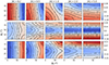Fig. 4. Color maps for each theoretical asymmetry parameter (top: a11, middle: a21, bottom: a22) for different values of ℛ. The solid (dashed) overplotted contours emphasize the values of the asymmetry parameters. Only the positive values of ℛ are shown since aℓ|m| are functions of ℛ2. There are symmetry relations of aℓ|m|(ℛ, 90° −βd, βq) = aℓ|m|(ℛ, 90° +βd, βq),aℓ|m|(ℛ, βd, 90° −βq) = aℓ|m|(ℛ, βd, 90° +βq) intrinsic to Eqs. (28)–(30); therefore, we limited βd and βq to the interval [0° ,90° ]. From left to right, the figure shows how the theoretical aℓ|m| vary with increasing |ℛ|.

3.3. Offset magnetic field

Lastly, we show the signature of an offset dipolar field (Case (c) in Fig. 1) on the splittings of the ℓ = 1 and ℓ = 2 oscillation modes, as observed at the surface of stars with radiative envelopes (Donati & Landstreet 2009; Vennes et al. 2017; Hardy et al. 2023a,b; Hollands et al. 2023). For this scenario, we directly use the numerical method, as the theoretical development of the asymmetry parameters becomes too convoluted for a proper derivation. The magsplitpy results are presented in Fig. 5 as a function of the offset z_o. We observe that, starting from a centered dipole, as we gradually offset the center of the field (increase z_o) up to the radius of the H-shell, all |a_ℓ|m|| converge to zero. This is because the magnetic field topology probed at the H-shell varies with z_o, going from purely dipolar to higher-order components when z_o increases. As a result, the magnetic field averages out along the H-shell, resulting in null asymmetries. Once z_o is greater than R_h, there are no longer radial magnetic field lines of opposite sign canceling out at the H-shell. As a result, |a_ℓ|m|| values increase, even though the field probed is of low amplitude (this increase depends on the geometry of the field, and might vary with the choice of the radial profile). Eventually, as z_o increases, the magnetic field amplitude at the H-shell decreases, and all |a_ℓ|m|| converge to zero again. We demonstrate through the model Case (c) that a small offset of a large-scale magnetic field along the rotation axis of about 3% of the extent of the radiative cavity leads to a disappearance of magnetic field effects on the symmetry of all the modes, due to the geometry of the H-shell. As a result, large-scale magnetic fields can have the same effect as small-scale magnetic fields (such as the one resulting from dynamo action; see, e.g., Fuller et al. 2019; Petitdemange et al. 2023).

Fig. 5. Asymmetry parameters aℓ, |m| depending on the offset of a magnetic field of type (c) in Fig. 1. The offset zo of the field is given relative to the radiative zone radius. The black dashed line indicates the location of the H-shell radius Rh.

4. Results and discussion

The following subsections are dedicated toward demonstrating the potential of ℓ = 2 mode splittings in lifting the topology degeneracy of the core magnetic field. The results of our study is meant to serve as a motivation for focused efforts to hunt for frequency splittings in ℓ = 2 mixed modes – which have been typically harder to detect than ℓ = 1 splitting due to small amplitudes. We first discuss the detectability of magnetic fields from ℓ = 2 mixed mode frequencies, and then develop on the path toward detecting mixed ℓ = 2 oscillation modes in Sect. 4.6.

4.1. Detectability of quadrudipole magnetic fields from ℓ = 1, 2 modes

From the results in Sect. 3, we demonstrate the detectability of quadrupolar magnetic field components from combined measurement on the ℓ = 1 and ℓ = 2 mixed mode frequencies. The top left panel of Fig. 6 presents three random examples of (ℛ, β) configuration in the case (a) of an aligned quadrudipole. The corresponding three asymmetry parameters are calculated, and their possible values to properly recover (ℛ, β) are represented in the β versus |ℛ| diagram in the other three panels. In the first step, we demarcate (with white lines) the exact degeneracies in (ℛ, β) when using measurement only one kind of asymmetry parameter (a₁₁ or a₂₁ or a₂₂). The shaded areas around the lines of the single a_ℓ|m| degeneracy represent the typical uncertainties that we analyze in Sect. 4.2.

Fig. 6. Overlapping bands of iso-asymmetry values across a11, a21, and a22 demonstrating the drastic reduction of degeneracy in (|ℛ|,β) space for a co-aligned quadrudipole when using ℓ = 1 and ℓ = 2 oscillation modes simultaneously. The white line, dashed line, and dashed-dotted line respectively indicate the analytical solution corresponding to the measurement of a11, a21, and a22 from Sect. 3.1. The width of colored bands indicating typical uncertainty on the measurement of the asymmetry parameters is chosen to account for the finite data frequency resolution of Kepler 4 years following Sect. 4.2.

For Star 1, taking one asymmetry parameter only (such as using only a₁₁ from measuring the frequency splittings in ℓ = 1 modes) leads to a total degeneracy of the quadrudipole with a purely dipolar field (as demonstrated by Mathis & Bugnet 2023). Adding a second asymmetry parameter (i.e., using ℓ = 2 modes) completely lifts this degeneracy, and both β and |ℛ| can be measured. Using the three asymmetry parameters confirms the measurement and allowed us to simultaneously extract exact measurements of β and |ℛ|. The same conclusion can be drawn for Star 2 if asymmetry parameters are known with high precision (see Sect. 4.2 for more details about uncertainties on asymmetry parameters). However, a null asymmetry parameter, as is the case for a₁₁ in the case of Star 3 where β ≈ 55°, is the worst-case scenario for a characterization of the magnetic field topology. Indeed, any small-scale magnetic field that averages out in the H-shell, or a nonmagnetic radiative zone, results in a null asymmetry parameter. It is therefore much harder to constrain the magnetic field topology for the field inclination angle nearing 55°, as illustrated in the bottom-right panel of Fig. 6.

4.2. Impact of the frequency resolution in the data on the degeneracy

As every asteroseismic measurement comes with its own uncertainty, we add in Fig. 6 the effect of the uncertainty on the measure of the asymmetry parameters on the inversion of β and |ℛ| through the shaded regions. The uncertainty on asymmetry parameters is calculated as (see Appendix E)

$$\begin{array}{c}\hfill \delta a_{\ell |m|}\approx \frac{\sqrt{6}\delta f}{\delta {\omega }_B^{\ell }},\end{array}$$(33)

with δf the frequency resolution in the data and $\delta {\omega }_B^{\ell }$ the averaged magnetic shift modulated by the ζ function as defined in Appendix E. For each of the chosen model stars in Sect. 4.1, we show patches of light, intermediate, and dark shades. The light-shaded area is indicative of the abundance of degenerate (|ℛ|,β) configurations on the availability of only one asymmetry parameter. The intermediate shaded region shows the reduced degeneracy constrained by using two asymmetry parameters. The darkest shade, which is the smallest patch, shows the restricted area in (|ℛ|,β) space when all three asymmetry parameters are available. We note that the shaded area increases with increasing data frequency resolution, here taken as 8nHz to mimic Kepler 4-year data resolution. As a result, the quality of data of course plays a major role in the detectability of complex magnetic field topology. Typical Kepler data uncertainty leads to a small degeneracy for Star 1, where the presence of a small quadrupolar component becomes debatable. The inclination angle β remains well-constrained. For Star 2, both the presence of the quadrupolar component and the inclination angle of the field remain well-constrained even with uncertainties on the asymmetry parameters. If Star 3 hosts a quadrudipole, it surely has a strong quadrupolar component and a well-constrained inclination angle near 55°, but the quadrupole to dipole strength ratio cannot be well constrained. This goes back to the discussion in Sect. 4.1 about near-zero asymmetry parameter values. In short, depending on the true (|ℛ|,β) parameters, the degeneracy regions can vary, and some stars might be more easily characterized than others.

The uncertainty on the a_ℓ|m| parameters from Eq. (33) is about 0.08 when taking ω_B^ℓ = 0.2 μHz. For |a_ℓ|m|| ranging from 0 up to 0.4, the minimum uncertainty associated with observational constraints with the Kepler mission is about 5%. As we demonstrated in Sect. 3.1.2, the error induced by the chosen methodology to compute asymmetry parameters is lower than 5% for a₁₁ and lower than 1% for a₂₁ and a₂₂, the dominant source of uncertainty on (|ℛ|,β) results indeed from observations and not from the chosen methodology.

4.3. Disentangling inclined quadrupoles

In Case (a), two out of three a_ℓ|m| are necessary to theoretically constrain the field topology through the measure of |ℛ| and β. In Case (b), however, three independent a_ℓ|m| are needed to fully constrain ℛ, β_d, and β_q. As a result of Appendix C, we note that a_ℓ|m| depend on each other through the relation

$$\begin{array}{c}\hfill a_{22}+a_{21}+\frac{5M_2^{0,0}}{\mathcal{T}\overline{B_r^2}(a_{11})}=1,\end{array}$$(34)

where $\overline{B_r^2}(a_{11})$ is an estimate of the horizontal average of the squared average magnetic field across the g-mode cavity obtained from the a₁₁ measurements using only ℓ = 1 modes. The term 𝒯 captures the integrated effect (in radius) of the mode sensitivity across the g-mode cavity in the radiative interior (see Eq. (C.7)), which is independent of field strength or topology. For a given field topology, $M_2^{0,0}$ takes a particular value (shift of the m = 0 quadrupolar mode). Therefore, the above equation with three asymmetry parameters only has two degrees of freedom, that is, the third asymmetry parameter is determined from the knowledge of the other two.

Therefore, we can only measure two independent asymmetry parameters to constrain the field topology. The degeneracy between the quadrudipole with or without inclination of the quadrupole with respect to the dipole axis is therefore not fully lifted when using ℓ = 1 and ℓ = 2 oscillation modes. Octupolar mixed-mode frequencies would be required, which are very unlikely to be detected in current datasets. Figure 7 shows the resulting degeneracies for the three stars in Fig. 6. For Star 1, assuming a quadrudipole configuration, we can deduce that (i) the dipole is inclined with a small angle with the rotation axis (β_d ≲ 25° ), (ii) that there is at least a small quadrupolar component ℛ, but (iii) the quadrupole can either be close to aligned with the dipole or close to a 90° inclination. For Star 2, the topology is much better constrained, with the dipole and quadrupole aligned with each other and the relative strength ℛ close to 1. Star 3 presents a full degeneracy in terms of the inclination angle of the dipole, while the ratio ℛ shows a dominant quadrupole with an axis of about 50° with respect to the dipole. Figure 7 has been simplified for readability; more comprehensive 2D degeneracy maps (see Fig. D.2) are discussed in Appendix D. Depending on the value of the asymmetry parameters, the degeneracy on the quadrudipole inclinations is therefore highly variable, and careful analyses will have to be performed on a case-by-case basis.

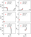Fig. 7. Degeneracies in the asymmetry parameters for the three stars in Fig. 6. Each column is a projection on the plane of two of the three field topology parameters (βq, βd), (βq, ℛ).

4.4. Impact of the centrality of the magnetic field on its detectability and characterization

We initiated in Sect. 3.3 a discussion regarding the impact of the centrality of large-scale magnetic fields on the observed asymmetries and therefore on the detectability of large-scale magnetic fields. In Fig. 8, we present the dependence of asymmetry parameters on inclination β_d of the dipole (solid lines and left axis) and on offset z_o (dashed lines and right axis). Even though a combination of the three asymmetry parameters is not perfectly the same in the case of inclined or the offset dipole, the solutions are very close to one another and lie within the uncertainty ranges from Appendix E. Signatures of the inclined dipole on the symmetry of each ℓ multiplet can therefore be degenerate with those of the offset dipole for β ⪅ 55° (see the pink regions in Fig. 8).

Fig. 8. Asymmetry parameters aℓ, |m| depending on the inclination angle of the field β in case (a) or on the offset of a magnetic field in the case (c) in Fig. 1. The offset zo of the field is given relative to the radiative zone radius. The pink region indicates, on each panel, the domain for which both an inclined dipole and an offset dipole can yield to the same asymmetry parameter. The blue and red stars show the minimum and maximum offsets measured from the combination of studies by Vennes et al. (2017), Hardy et al. (2023a,b), Hollands et al. (2023). J0942+2052 has an offset of −0.01 (Hardy et al. 2023b) and J0017+004 of 0.40 (Hardy et al. 2023a).

Star 1 from Fig. 6 has asymmetry parameter values such as the field can be a quadrudipole inclined with a dipole angle of β_d = 25° and |ℛ| of about 0.5 as in Fig. 6. However, a purely dipolar field with an offset along the rotation axis of about 2% of the radiative zone extent leads to very similar asymmetry values (see Fig. 8). Including measurement uncertainties as described in Appendix E, the offset dipole and the quadrudipole corresponding to the asymmetry parameters of Star 1 would be degenerate. For Star 2 and Star 3, quadrudipoles with the configurations discussed previously are not degenerated with an offset dipolar field, as the a₂₁ parameter corresponding to the quadrudipoles cannot be recovered with a dipolar field (offset or not, see Fig. 3).

Additionally, we also include upper and lower boundaries of offsets observed in white dwarfs for comparison. The minimum amd maximum observed z_o values are taken from Vennes et al. (2017), Hardy et al. (2023a,b), Hollands et al. (2023). The red star (J0017+004) corresponding to z_o = 0.4 leads to near zero asymmetry parameter values; it would be very hard to detect such a magnetic field geometry from asymmetries, and one would have to rely only on the global shifts ω_B^ℓ. The blue star (J0942+2052), corresponding to an offset of |z_o| = 0.01 is close to be degenerated with a centered dipole, but the three asymmetry parameters would each lead to a different β_ℓ|m| angle. To understand this in the more general case, we calculate all asymmetry parameters a₁₁(z_o),a₂₁(z_o),a₂(z_o) for a fixed offset z_o. Then, we calculate for each asymmetry parameter the corresponding inclination angles β_ℓ|m|. These three inclination angles for different a_ℓ|m| might not be the same, and their differences are presented in Fig. 9. When the difference in angles is non-zero the combination of asymmetry parameters is unique to an offset dipole and can be distinguished from an inclined dipole, which is the case for J0942+2052 but not for J0017+0041, which is fully degenerate. This result has to be discussed in perspective with current uncertainties on the measure of asymmetry parameters (see Appendix E). For instance, observations from Li et al. (2022) lead to an uncertainty in the inclination angle of ∼ ± 7° (see also Mathis & Bugnet 2023), which is higher than the largest difference in β angles measured from asymmetry parameters in Fig. 9. As a result, even though asymmetry parameters are not perfectly identical from the two configurations, it might be complicated to distinguish between a centered dipole and an offset one based on asymmetry parameter values with associated observational uncertainties.

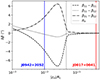Fig. 9. Differences between the inclination angles resulting from the asymmetry parameters of different offsets.

The average shift ω_B^ℓ depends on the squared averaged magnetic field strength at the H-shell as well, which makes it sensitive to only this particular layer. Strong offset magnetic fields might therefore be confused for weaker centered fields when using ω_B^ℓ and a_ℓ|m|. This implies that magnetic fields might be underestimated in red giant cores, as a stronger offset dipole can have the same signature on the ℓ = 1 asymmetry parameter than a weaker centered dipole (valid also for ℓ = 2). As a result, one should be careful when extracting a magnetic field amplitude from ω_B^ℓ, which should rather be taken as a minimum amplitude of the large-scale field.

4.5. Accessing asymmetry parameters

As demonstrated by Gough & Thompson (1990) and more recently by Loi (2021), magnetic fields with a high inclination with respect to the rotation axis generate a second lift of degeneracy of the mixed mode frequencies in the observer frame. The relative amplitude of these additional components of the mixed-mode multiplets compared to the central peaks studied here strongly depends on the magnetic field amplitude. As we place our study in the case of rotation-dominated signatures, these additional multiplet components contain a small fraction of the mode power density (Loi 2021) and have therefore been neglected in our study. As a second result of this approximation, we could neglect the effect of magnetic fields on the mode amplitudes. Therefore, we assumed that the amplitudes in mixed mode multiplets are consistent with the study of Gizon & Solanki (2003) in the case of pure rotation (further justified by the study of Loi 2021, in the case of weak magnetic fields).

As discussed in Gizon & Solanki (2003), all components of a given (ℓ,m) multiplet are not visible simultaneously, depending on the line of sight of the observation. This makes the detectability of complex magnetic fields challenging, as we cannot access all asymmetry parameters simultaneously. Following Appendix C, assuming that magnetic fields are at play, the average shift of the ℓ = 2 multiplet ${\omega }_B^{\ell =2}$ can always be estimated when two out of the three |m| components are visible. As a result, for a given inclination angle i ⪆ 10°, at least two components of the ℓ = 2 mixed mode multiplet are visible (Gizon & Solanki 2003), which result in a systematic estimate for ${\omega }_B^{\ell }$ (i.e., the denominator in Eq. (10)) when i ⪆ 10°. However, only asymmetry parameters corresponding to the visible components of the multiplet are simultaneously measurable, which depends on i. In Table 1 we report the detectability of the various asymmetry parameters given the inclination of the line of sight i with respect to the rotation axis. Table 1 shows that we have access to two asymmetry parameters (or of their combination) for most of the inclination angles of the observations ([a₁₁ and a₂₁] for 10 ⪅ i ⪅ 40°, [a₁₁ and a₂₂ − a₂₁] for 40 ⪅ i ⪅ 70°, and [a₂₁ and a₂₂] for 70 ⪅ i ⪅ 80°). From Fig. 6 we observe that having access to only one out of the two ℓ = 2 asymmetry parameters or to their combination is theoretically enough as a₁₁, a₂₁, and a₂₂ are not independent (see Appendix C). In a realistic scenario, depending on errors in the measure of the visible asymmetries, two asymmetry parameters might be enough to partially lift the topology degeneracy. The resulting degeneracy depends on the true (ℛ, β) combination (see Fig. 6 in the case of the aligned quadrudipole). We conclude that topologies might be unveiled from ℓ = 1, 2 frequencies following our study for stars observed with an inclination angle 10 ⪅ i ⪅ 80° when assuming rotation effects dominating magnetic effects. The full investigation of the effect of stronger magnetic fields on the amplitudes and detectability of the different components of the multiplet given the line of sight will be the scope of a follow-up paper.

4.6. The challenge of ℓ = 2 mixed modes detection

Due to the low coupling between acoustic and gravity quadrupolar modes, ℓ = 2 g-dominated mixed modes have a very low amplitude. As a result, ℓ = 2 mixed modes (sensitive to red giant core magnetism) are extremely difficult to identify, and measuring frequency splitting on these mixed modes is even more difficult (e.g., Ahlborn et al. 2020). While we are aware of these challenges, efforts toward dedicated search for ℓ = 2 mixed modes in red giants should be one of the major focus in red giant asteroseismology.

A crucial first step is to identify stellar candidates showing promising magnetic signatures. Stars already known to be magnetic from studying their ℓ = 1 modes are prime candidates. In addition, adapting global detection methods specifically designed for magnetism (such as the modified stretching of g-mode period spacing using the ΔΠ₁ method for ℓ = 1 modes as derived in Bugnet 2022) to ℓ = 2 modes would serve as yet another effective precursor of magnetic signature in ℓ = 2 modes. These two-steps approach of fitting the power spectra to identify ℓ = 2 magnetic signatures should be relatively simpler than a direct fitting approach to detect ℓ = 2 mixed modes.

After these prior screening steps to extract a gold sample of candidates, the final step would require a fine analysis of the frequency in the ℓ = 2 regions. The past few years have seen considerable advancement in sophisticated data analysis methods, but no study implementing these methods to the detectability of ℓ = 2 mixed modes has been conducted recently. With a surge of softwares suitable for highly efficient parallelized computation across multiple CPU nodes such as emcee (Foreman-Mackey 2019) and JAX (Bradbury et al. 2018), we can now utilize powerful optimization tools using Bayesian frameworks to identify modes. Bayesian methods have already started gaining applications in asteroseismology, as done in identifying rotationally split ℓ = 1 mixed modes (e.g., Kuszlewicz et al. 2023; Li et al. 2024). Efficient machine learning algorithms (Hon et al. 2017, 2018, 2019; Dhanpal et al. 2022, 2023) to identify mixed mode frequency and period separation is yet another coming-of-the-age tool that may be harnessed to fit for ℓ = 2 modes with magnetic signatures.

In addition to efficient new analysis tools, the most important change that has happened over the past few years is that asteroseismologists are no longer blind to signatures expected from magnetized red giants. These serve as crucial priors and constraints for Bayesian and deep learning frameworks mentioned above. The symmetric splitting of ℓ = 1 modes inform rotation and the asymmetric splitting informs magnetism (and second order effects of rotation, if significant). These constitute vital priors for ℓ = 2 rotational splittings and asymmetry parameters a_2|m|, which are required for the full characterization of ℓ = 2 modes. A specific example of a constraining equation is Eq. (34), which effectively passes on the information of the measured average radial field $\overline{B_r^2(a_{11})}$ from the ℓ = 1 asymmetry parameter a₁₁ to the measurement of asymmetric splitting of ℓ = 2 modes. Therefore, a fitting routine for ℓ = 2 modes would account for all of this prior information for stars that carry magnetic signatures in ℓ = 1 modes. Such fitting routines would be much more constrained, which should facilitate magnetic detection in ℓ = 2 modes in stars where ℓ = 1 modes carry magnetic signatures.

5. Conclusion and perspectives

We have demonstrated that a combined analysis of ℓ = 1 and ℓ = 2 mixed mode frequency asymmetries is key to accessing the quadrupolar component of magnetic fields. When using asymmetry parameters associated with (ℓ = 1, |m| = 1), (ℓ = 2, |m| = 1), and (ℓ = 2, |m| = 2) frequencies, the degeneracy between the signature of aligned and centered dipolar and quadrupolar components of the field can be lifted, allowing their respective strength to be measured (depending on the resolution in the data). Aligned quadrupolar fields can therefore be detected from the study of ℓ = 2 oscillation modes. Depending on the inclination of the quadrupole with respect to the dipole, a misalignment might or might not be constrained from ℓ = 1 and ℓ = 2 frequencies.

As the observed magnetic fields in white dwarfs and main-sequence intermediate stars show offset fields (e.g., Wickramasinghe & Ferrario 2000; Hardy et al. 2023b), we also investigated the detectability of such topologies. We have demonstrated that strong offset fields can be confused with weaker and centered fields and that we do not currently have a way to distinguish between them. As a result, the magnetic field amplitudes estimated from shifts in the frequency pattern should be considered a lower boundary for the true magnetic field amplitude in the radiative zone.

Depending on the inclination of the rotation axis of the star with respect to the line of sight, some asymmetry parameters might not be measurable due to a low amplitude in |m| components (Gizon & Solanki 2003; Gehan et al. 2021). Our results therefore apply to stars observed with a line of sight i ∈ [10, 80]° (which is the case for most observed stars) and rotation effects dominating magnetic effects, which is the case for magnetic red giants detected so far (Li et al. 2022; Deheuvels et al. 2023; Li et al. 2023).

While we have derived these magnetoasteroseismology prescriptions for both ℓ = 1 and ℓ = 2 modes, ℓ = 2 mixed oscillation frequencies are extremely complicated to identify in asteroseismic data (e.g., Ahlborn et al. 2020). For this reason, there has not been a dedicated quest for the characterization of quadrupolar mixed modes in the thousands of red giants observed by Kepler, and it is thus lacking in the literature on red giant stars. Considering the stars for which the rotation and magnetic fields have been measured from ℓ = 1 oscillations, forward modeling of the rotating and magnetic mixed-mode patterns including the magnetic effects of topologies discussed above for ℓ = 2 modes could be the solution to identify and take advantage of ℓ = 2 frequencies and obtain a better constraint on the angular momentum transport inside stars.

Data availability

The MESA inlist file is available at https://doi.org/10.5281/zenodo.12804810

Acknowledgments

The authors thank S. Mathis, L. Barrault, S. Torres, A. Cristea, and K. M. Smith for very useful discussions. This project has received funding from the European Union’s Horizon 2020 research and innovation programme under the Marie Skłodowska-Curíe grant agreement No 101034413. The authors thank the anonymous referee for valuable comments and suggestions to improve the manuscript.

References

Appendix A: B_r expression for an inclined quadrudipole

We briefly outline the mathematical steps to derive the expression of B_r for a general quadrudipole, where the dipolar and quadrupolar axes are not necessarily aligned. The schematic representation of a general quadrudipole is shown in Fig. 1. The dipole is inclined at an angle β_d to the rotation axis and the quadrupole is inclined at an angle β_q to the rotation axis. To go about constructing this, let’s start at the simpler case where the symmetry axis of the dipole and quadrupole are aligned with the rotation axis. The expression for the radial field component in this case will look like

$$\begin{array}{c}\hfill B_r(r,\theta ,\varphi )=B_0{b}_r(r)[Y_{10}(\theta ,\phi )+\mathcal{R}{Y}_{20}(\theta ,\phi )],\end{array}$$(A.1)

where ℛ is the ratio of the strength of the quadrupole to the dipole. Now, we want to incline the dipolar component by an angle β_d with respect to the rotation axis. For this, let’s first choose a frame $({\stackrel{\sim }{\theta }}_d,{\stackrel{\sim }{\phi }}_d)$ where the dipole is axisymmetric and then find the coordinate transform between $({\stackrel{\sim }{\theta }}_d,{\stackrel{\sim }{\phi }}_d)$ and (θ, φ). Thanks to Wigner d-matrices (Varshalovich et al. 1988), we can use the following relation to go from the axisymmetric frame to a non-axisymmetric frame rotated by β:

$$\begin{array}{c}\hfill Y_{\ell ,m}(\theta ,\phi )=d_{m,0}^{(\ell )}({\beta }_d)Y_{\ell ,0}({\theta }_d,{\phi }_d).\end{array}$$(A.2)

Then, using the fact that Wigner d-matrices are unitary, we get the expression

$$\begin{array}{c}\hfill Y_{\ell ,0}({\theta }_d,{\phi }_d)={\displaystyle \sum _{m=-\ell }^{\ell }}{d}_{0,m}^{(\ell )}({\beta }_d)Y_{\ell ,m}(\theta ,\phi ).\end{array}$$(A.3)

So, for a dipole inclined at β_d from the rotation axis and a quadrupole aligned with the rotation axis, the expression for the radial component of the magnetic field reads

$$\begin{array}{cc}\hfill B_r(r,\theta ,\varphi )& =B_0{b}_r(r)[Y_{10}({\theta }_d,{\phi }_d)+\mathcal{R}{Y}_{20}(\theta ,\phi )],\hfill \\ \hfill & =B_0{b}_r(r)[{\displaystyle \sum _{m=-1}^1}{d}_{0,m}^{(1)}({\beta }_d)Y_{1,m}(\theta ,\phi )+\mathcal{R}{Y}_{20}(\theta ,\phi )].\hfill \end{array}$$(A.4)

Similarly, the transformation between a coordinate that is rotated by β_q (where the quadrupole is axisymmetric) and the coordinate of axisymmetric rotation is given by

$$\begin{array}{c}\hfill Y_{\ell ,0}({\theta }_q,{\phi }_q)={\displaystyle \sum _{m=-\ell }^{\ell }}{d}_{0,m}^{(\ell )}({\beta }_q)Y_{\ell ,m}(\theta ,\phi ).\end{array}$$(A.5)

Therefore, the total B_r(r, θ, φ) where the dipole and quadrupole are tilted by β_d and β_q with respect to the rotation axis is given by

$$\begin{array}{cc}\hfill B_r(r,\theta ,\phi )=B_0{b}_r(r)({\displaystyle \sum _{m=-1}^1}& d_{0,m}^{(1)}({\beta }_d)Y_{1m}(\theta ,\phi )\hfill \\ \hfill +& \mathcal{R}{\displaystyle \sum _{m=-2}^2}{d}_{0,m}^{(2)}({\beta }_q)Y_{2m}(\theta ,\phi )).\hfill \end{array}$$(A.6)

On plugging in the elements of the Wigner d-matrices, in Eq. A.6, we get the expression in Eq. 15.

Appendix B: Magnetic inversion kernels

Section 2.4 outlines the numerical approach we adopt to calculate the magnetic coupling matrix. A key component in the numerical evaluation of magnetically perturbed stellar eigenstates is its Lorentz-stress sensitivity kernels (originally laid out in Das et al. 2020). These Lorentz-stress kernel components ${}_{k\prime k}{\mathcal{B}}_{\mathit{st}}^{\mu \nu }$ in Eq. 19, are defined as

$$\begin{array}{c}\hfill {}_{k^{\prime }k}{\mathcal{B}}_{\mathit{st}}^{\mu \nu }=4\pi {(-1)}^{m^{\prime }}{\gamma }_{{\ell }^{\prime }}{\gamma }_s{\gamma }_{\ell }(\begin{array}{ccc}{\ell }^{\prime }& s& \ell \\ -m^{\prime }& t& m\end{array}){}_{k^{\prime }k}{\mathcal{G}}_s^{\mu \nu },\end{array}$$(B.1)

where ${\gamma }_{\ell }=\sqrt{2\ell +1/4\pi }$ and $(\begin{array}{c}\ell \prime s\ell \\ -m\prime tm\end{array})$ are the Wigner 3-j symbols obtained from triple product of complex spherical harmonics (see Appendix C of Dahlen & Tromp 1999). The m independent part of the kernels ${}_{k\prime k}{\mathcal{G}}_s^{\mu \nu }$ are functions of the stellar eigenfunctions (hence the structure of the background stellar model):

$$\begin{array}{cc}\hfill {\mathcal{G}}_s^{--}=& \frac{-1}{2r^2}[(\begin{array}{ccc}{\ell }^{\prime }& s& \ell \\ 2& -2& 0\end{array}){\chi }_1^{--}(k,k^{\prime })+(\begin{array}{ccc}{\ell }^{\prime }& s& \ell \\ 0& -2& 2\end{array}){\chi }_1^{--}(k^{\prime },k)\hfill \\ \hfill & +(\begin{array}{ccc}{\ell }^{\prime }& s& \ell \\ 1& -2& 1\end{array})\{{\chi }_2^{--}(k,k^{\prime })+{\chi }_2^{--}(k^{\prime },k)\}\hfill \\ \hfill & +(\begin{array}{ccc}{\ell }^{\prime }& s& \ell \\ 3& -2& -1\end{array}){\chi }_3^{--}(k,k^{\prime })+(\begin{array}{ccc}{\ell }^{\prime }& s& \ell \\ -1& -2& 3\end{array}){\chi }_3^{--}(k^{\prime },k)],\hfill \end{array}$$(B.2)

$$\begin{array}{cc}\hfill {\mathcal{G}}_s^{0-}=& \frac{1}{4r^2}[(\begin{array}{ccc}{\ell }^{\prime }& s& \ell \\ 1& -1& 0\end{array}){\chi }_1^{0-}(k,k^{\prime })+(\begin{array}{ccc}{\ell }^{\prime }& s& \ell \\ 0& -1& 1\end{array}){\chi }_1^{0-}(k^{\prime },k)\hfill \\ \hfill & +(\begin{array}{ccc}{\ell }^{\prime }& s& \ell \\ -1& -1& 2\end{array}){\chi }_2^{0-}(k,k^{\prime })+(\begin{array}{ccc}{\ell }^{\prime }& s& \ell \\ 2& -1& -1\end{array}){\chi }_2^{0-}(k^{\prime },k)],\hfill \end{array}$$(B.3)

$$\begin{array}{cc}\hfill {\mathcal{G}}_s^{00}=& \frac{1}{2r^2}(1+p)\{\frac{1}{2}(\begin{array}{ccc}{\ell }^{\prime }& s& \ell \\ 0& 0& 0\end{array})[{\chi }_1^{00}(k,k^{\prime })+{\chi }_1^{00}(k^{\prime },k)]\hfill \\ \hfill & +(\begin{array}{ccc}{\ell }^{\prime }& s& \ell \\ -1& 0& 1\end{array})[{\chi }_2^{00}(k,k^{\prime })+{\chi }_2^{00}(k^{\prime },k)]\},\hfill \end{array}$$(B.4)

$$\begin{array}{cc}\hfill {\mathcal{G}}_s^{+-}=& \frac{1}{4r^2}(1+p)\{\frac{1}{2}(\begin{array}{ccc}{\ell }^{\prime }& s& \ell \\ 0& 0& 0\end{array})[{\chi }_1^{+-}(k,k^{\prime })+{\chi }_1^{+-}(k^{\prime },k)]\hfill \\ & +(\begin{array}{ccc}{\ell }^{\prime }& s& \ell \\ -2& 0& 2\end{array})[{\chi }_2^{+-}(k,k^{\prime })+{\chi }_2^{+-}(k^{\prime },k)]\hfill \\ & +(\begin{array}{ccc}{\ell }^{\prime }& s& \ell \\ -1& 0& 1\end{array})[{\chi }_3^{+-}(k,k^{\prime })+{\chi }_3^{+-}(k^{\prime },k)]\},\hfill \end{array}$$(B.5)

where p = ( − 1)^{ℓ + ℓ′+s} and

$$\begin{array}{cc}\hfill {\chi }_1^{--}(k)& ={\mathrm{\Omega }}_{0\ell }{\mathrm{\Omega }}_{2\ell }[V_k(3U_k-2{\mathrm{\Omega }}_{2\ell }^2{V}_k+3r\dot{U_k})-r{U}_k\dot{V_k}],\hfill \end{array}$$(B.6)

$$\begin{array}{cc}\hfill {\chi }_2^{--}(k)& ={\mathrm{\Omega }}_{0\ell }^2[3U_k{V}_k+({\mathrm{\Omega }}_{2\ell }^2-2{\mathrm{\Omega }}_{0\ell }^2)V_k^2+r{V}_k\dot{U_k}-r{U}_k\dot{V_k}-U_k^2],\hfill \end{array}$$(B.7)

$$\begin{array}{cc}\hfill {\chi }_3^{--}(k)& ={\mathrm{\Omega }}_{0\ell }^2{\mathrm{\Omega }}_{2\ell }{\mathrm{\Omega }}_{3\ell }{V}_k^2,\hfill \end{array}$$(B.8)

$$\begin{array}{cc}\hfill {\chi }_1^{0-}(k)& ={\mathrm{\Omega }}_{0\ell }[4{\mathrm{\Omega }}_{0\ell }^2{V}_k^2-4r{\mathrm{\Omega }}_{0\ell }^2{V}_k\dot{V_k}+2r^2\dot{U_k}\dot{V_k}+r^2{V}_k\ddot{U_k}\hfill \\ \hfill & +U_k\{8U_k-6({\mathrm{\Omega }}_{0\ell }^2+1)V_k+r(4\dot{V_k}-r\ddot{V_k})\}],\hfill \end{array}$$(B.9)

$$\begin{array}{cc}\hfill {\chi }_2^{0-}(k)& ={\mathrm{\Omega }}_{0\ell }^2{\mathrm{\Omega }}_{2\ell }[U_k{V}_k+V_k(U_k-4V_k+3r\dot{V_k})+r{V}_k\dot{V_k}],\hfill \end{array}$$(B.10)

$$\begin{array}{cc}\hfill {\chi }_1^{00}(k)& =2[-2r{U}_k\dot{U_k}+{\mathrm{\Omega }}_{0\ell }^{2}r(V_k\dot{U_k}+U_k\dot{V_k})\hfill \\ \hfill & -5{\mathrm{\Omega }}_{0\ell }^2{V}_k{U}_k+2{\mathrm{\Omega }}_{0\ell }^4{V}_k^2+3U_k^2],\hfill \end{array}$$(B.11)

$$\begin{array}{cc}\hfill {\chi }_2^{00}(k)& =-{\mathrm{\Omega }}_{0\ell }^2[-U_k{V}_k+V_k^2+r(V_k\dot{U_k}+U_k\dot{V_k})\hfill \end{array}$$(B.12)

$$\begin{array}{cc}& -2r{V}_k\dot{V_k}+r^2{\dot{V_k}}^2],\hfill \end{array}$$(B.13)

$$\begin{array}{cc}\hfill {\chi }_1^{+-}(k)& =2[-2r\dot{U_k}{U}_k+{\mathrm{\Omega }}_{0\ell }^{2}r(\dot{U_k}{V}_k+U_k\dot{V_k})-r^2{\dot{U_k}}^2\hfill \\ \hfill & -{\mathrm{\Omega }}_{0\ell }^2{U}_k{V}_k+U_k^2],\hfill \end{array}$$(B.14)

$$\begin{array}{cc}\hfill {\chi }_2^{+-}(k)& =-2{\mathrm{\Omega }}_{0\ell }^2{\mathrm{\Omega }}_{2\ell }^2{V}_k^2,\hfill \end{array}$$(B.15)

$$\begin{array}{cc}\hfill {\chi }_3^{+-}(k)& ={\mathrm{\Omega }}_{0\ell }^2[r(U_k\dot{V_k}-V_k\dot{U_k})-U_k{V}_k+U_k^2],\hfill \end{array}$$(B.16)

References

- Ahlborn, F., Bellinger, E. P., Hekker, S., Basu, S., & Angelou, G. C. 2020, A&A, 639, A98 [NASA ADS] [CrossRef] [EDP Sciences] [Google Scholar]
- Beck, P. G., Montalban, J., Kallinger, T., et al. 2012, Nature, 481, 55 [Google Scholar]
- Beuermann, K., Euchner, F., Reinsch, K., Jordan, S., & Gänsicke, B. T. 2007, A&A, 463, 647 [NASA ADS] [CrossRef] [EDP Sciences] [Google Scholar]
- Bhattacharya, S., Bharati Das, S., Bugnet, L., Panda, S., & Hanasoge, S. M. 2024, ApJ, 970, 24 [NASA ADS] [CrossRef] [Google Scholar]
- Bradbury, J., Frostig, R., Hawkins, P., et al. 2018, JAX: composable transformations of Python + NumPy programs [Google Scholar]
- Braithwaite, J. 2008, MNRAS, 386, 1947 [Google Scholar]
- Broderick, A. E., & Narayan, R. 2008, MNRAS, 383, 943 [Google Scholar]
- Bugnet, L. 2022, A&A, 667, A68 [NASA ADS] [CrossRef] [EDP Sciences] [Google Scholar]
- Bugnet, L., Prat, V., Mathis, S., et al. 2021, A&A, 650, A53 [NASA ADS] [CrossRef] [EDP Sciences] [Google Scholar]
- Ceillier, T., Eggenberger, P., García, R. A., & Mathis, S. 2013, A&A, 555, A54 [NASA ADS] [CrossRef] [EDP Sciences] [Google Scholar]
- Dahlen, F. A., & Tromp, J. 1999, Theoretical Global Seismology (Princeton University Press) [Google Scholar]
- Das, S. B., Chakraborty, T., Hanasoge, S. M., & Tromp, J. 2020, ApJ, 897, 38 [NASA ADS] [CrossRef] [Google Scholar]
- Deheuvels, S., García, R. A., Chaplin, W. J., et al. 2012, ApJ, 756, 19 [Google Scholar]
- Deheuvels, S., Dogan, G., Goupil, M. J., et al. 2014, A&A, 564, A27 [NASA ADS] [CrossRef] [EDP Sciences] [Google Scholar]
- Deheuvels, S., Ballot, J., Beck, P. G., et al. 2015, A&A, 580, A96 [NASA ADS] [CrossRef] [EDP Sciences] [Google Scholar]
- Deheuvels, S., Ouazzani, R. M., & Basu, S. 2017, A&A, 605, A75 [NASA ADS] [CrossRef] [EDP Sciences] [Google Scholar]
- Deheuvels, S., Ballot, J., Eggenberger, P., et al. 2020, A&A, 641, A117 [EDP Sciences] [Google Scholar]
- Deheuvels, S., Li, G., Ballot, J., & Ligniéres, F. 2023, A&A, 670, L16 [NASA ADS] [CrossRef] [EDP Sciences] [Google Scholar]
- Dhanpal, S., Benomar, O., Hanasoge, S., et al. 2022, ApJ, 928, 188 [NASA ADS] [CrossRef] [Google Scholar]
- Dhanpal, S., Benomar, O., Hanasoge, S., et al. 2023, ApJ, 958, 63 [NASA ADS] [CrossRef] [Google Scholar]
- Di Mauro, M. P., Ventura, R., Cardini, D., et al. 2016, ApJ, 817, 65 [NASA ADS] [CrossRef] [Google Scholar]
- Donati, J.-F., & Landstreet, J. 2009, ARA&A, 47, 333 [NASA ADS] [CrossRef] [Google Scholar]
- Duez, V., & Mathis, S. 2010, A&A, 517, A58 [NASA ADS] [CrossRef] [EDP Sciences] [Google Scholar]
- Eggenberger, P., Haemmerlé, L., Meynet, G., & Maeder, A. 2012, A&A, 539, A70 [NASA ADS] [CrossRef] [EDP Sciences] [Google Scholar]
- Eggenberger, P., Moyano, F. D., & den Hartogh, J. W. 2022, A&A, 664, L16 [NASA ADS] [CrossRef] [EDP Sciences] [Google Scholar]
- Euchner, F., Reinsch, K., Jordan, S., Beuermann, K., & Gänsicke, B. T. 2005, A&A, 442, 651 [NASA ADS] [CrossRef] [EDP Sciences] [Google Scholar]
- Euchner, F., Jordan, S., Beuermann, K., Reinsch, K., & Gänsicke, B. T. 2006, A&A, 451, 671 [NASA ADS] [CrossRef] [EDP Sciences] [Google Scholar]
- Foreman-Mackey, D. 2019, Astrophysics Source Code Library [record ascl:1910.005] [Google Scholar]
- Fuller, J., Piro, A. L., & Jermyn, A. S. 2019, MNRAS, 485, 3661 [NASA ADS] [Google Scholar]
- Gehan, C., Mosser, B., Michel, E., Samadi, R., & Kallinger, T. 2018, A&A, 616, A24 [NASA ADS] [CrossRef] [EDP Sciences] [Google Scholar]
- Gehan, C., Mosser, B., Michel, E., & Cunha, M. S. 2021, A&A, 645, A124 [NASA ADS] [CrossRef] [EDP Sciences] [Google Scholar]
- Gizon, L., & Solanki, S. K. 2003, ApJ, 589, 1009 [Google Scholar]
- Gomes, P., & Lopes, I. 2020, MNRAS, 496, 620 [NASA ADS] [CrossRef] [Google Scholar]
- Gough, D. O., & Thompson, M. J. 1990, MNRAS, 242, 25 [Google Scholar]
- Goupil, M. J., Mosser, B., Marques, J. P., et al. 2013, A&A, 549, A75 [NASA ADS] [CrossRef] [EDP Sciences] [Google Scholar]
- Hardy, F., Dufour, P., & Jordan, S. 2023a, MNRAS, 520, 6111 [CrossRef] [Google Scholar]
- Hardy, F., Dufour, P., & Jordan, S. 2023b, MNRAS, 520, 6135 [CrossRef] [Google Scholar]
- Hatt, E. J., Ong, J. M. J., Nielsen, M. B., et al. 2024, MNRAS, 534, 1060 [NASA ADS] [CrossRef] [Google Scholar]
- Hollands, M. A., Stopkowicz, S., Kitsaras, M. P., et al. 2023, MNRAS, 520, 3560 [NASA ADS] [CrossRef] [Google Scholar]
- Hon, M., Stello, D., & Yu, J. 2017, MNRAS, 469, 4578 [NASA ADS] [CrossRef] [Google Scholar]
- Hon, M., Stello, D., & Zinn, J. C. 2018, ApJ, 859, 64 [NASA ADS] [CrossRef] [Google Scholar]
- Hon, M., Stello, D., García, R. A., et al. 2019, MNRAS, 485, 5616 [NASA ADS] [Google Scholar]
- Jermyn, A. S., Bauer, E. B., Schwab, J., et al. 2023, ApJS, 265, 15 [NASA ADS] [CrossRef] [Google Scholar]
- Kochukhov, O., Papakonstantinou, N., & Neiner, C. 2022, MNRAS, 510, 5821 [NASA ADS] [CrossRef] [Google Scholar]
- Kuszlewicz, J. S., Hon, M., & Huber, D. 2023, ApJ, 954, 19 [NASA ADS] [CrossRef] [Google Scholar]
- Landstreet, J. D., Bagnulo, S., Valyavin, G., & Valeev, A. F. 2017, A&A, 607, A92 [NASA ADS] [CrossRef] [EDP Sciences] [Google Scholar]
- Li, G., Deheuvels, S., Ballot, J., & Ligniéres, F. 2022, Nature, 610, 43 [NASA ADS] [CrossRef] [Google Scholar]
- Li, G., Deheuvels, S., Li, T., Ballot, J., & Lignieres, F. 2023, A&A, 680, A26 [NASA ADS] [CrossRef] [EDP Sciences] [Google Scholar]
- Li, G., Deheuvels, S., & Ballot, J. 2024, A&A, 688, A184 [NASA ADS] [CrossRef] [EDP Sciences] [Google Scholar]
- Loi, S. T. 2020, MNRAS, 496, 3829 [Google Scholar]
- Loi, S. T. 2021, MNRAS, 504, 3711 [NASA ADS] [CrossRef] [Google Scholar]
- Loi, S. T., & Papaloizou, J. C. B. 2020, MNRAS, 491, 708 [Google Scholar]
- Marques, J. P., Goupil, M. J., Lebreton, Y., et al. 2013, A&A, 549, A74 [NASA ADS] [CrossRef] [EDP Sciences] [Google Scholar]
- Mathis, S., & Bugnet, L. 2023, A&A, 676, L9 [NASA ADS] [CrossRef] [EDP Sciences] [Google Scholar]
- Mathis, S., & Zahn, J. P. 2005, A&A, 440, 653 [NASA ADS] [CrossRef] [EDP Sciences] [Google Scholar]
- Mathis, S., Bugnet, L., Prat, V., et al. 2021, A&A, 647, A122 [EDP Sciences] [Google Scholar]
- Maxted, P. F. L., Ferrario, L., Marsh, T. R., & Wickramasinghe, D. T. 2000, MNRAS, 315, L41 [NASA ADS] [CrossRef] [Google Scholar]
- Mestel, L., & Weiss, 1987, MNRAS, 226, 123 [CrossRef] [Google Scholar]
- Mosser, B., Elsworth, Y., Hekker, S., et al. 2012, A&A, 537, A30 [NASA ADS] [CrossRef] [EDP Sciences] [Google Scholar]
- Moyano, F. D., Eggenberger, P., Salmon, S. J. A. J., Mombarg, J. S. G., & Ekström, S. 2023, A&A, 677, A6 [NASA ADS] [CrossRef] [EDP Sciences] [Google Scholar]
- Paxton, B., Bildsten, L., Dotter, A., et al. 2011, ApJS, 192, 3 [Google Scholar]
- Paxton, B., Cantiello, M., Arras, P., et al. 2013, ApJS, 208, 4 [Google Scholar]
- Paxton, B., Marchant, P., Schwab, J., et al. 2015, ApJS, 220, 15 [Google Scholar]
- Paxton, B., Schwab, J., Bauer, E. B., et al. 2018, ApJS, 234, 34 [NASA ADS] [CrossRef] [Google Scholar]
- Paxton, B., Smolec, R., Schwab, J., et al. 2019, ApJS, 243, 10 [Google Scholar]
- Petitdemange, L., Marcotte, F., & Gissinger, C. 2023, Science, 379, 300 [NASA ADS] [CrossRef] [Google Scholar]
- Pijpers, F. P., Di Mauro, M. P., & Ventura, R. 2021, A&A, 656, A151 [NASA ADS] [CrossRef] [EDP Sciences] [Google Scholar]
- Prat, V., Mathis, S., Buysschaert, B., et al. 2019, A&A, 627, A64 [NASA ADS] [CrossRef] [EDP Sciences] [Google Scholar]
- Seach, J. M., Marsden, S. C., Carter, B. D., et al. 2020, MNRAS, 494, 5682 [Google Scholar]
- Silvester, J., Kochukhov, O., Rusomarov, N., & Wade, G. A. 2017, MNRAS, 471, 962 [NASA ADS] [CrossRef] [Google Scholar]
- Spruit, H. C. 1999, A&A, 349, 189 [NASA ADS] [Google Scholar]
- Spruit, H. C. 2002, A&A, 381, 923 [CrossRef] [EDP Sciences] [Google Scholar]
- Tayar, J., Beck, P. G., Pinsonneault, M. H., García, R. A., & Mathur, S. 2019, ApJ, 887, 2 [Google Scholar]
- Tayler, R. 1980, MNRAS, 191, 151 [Google Scholar]
- Townsend, R. H., & Teitler, S. A. 2013, MNRAS, 435, 3406 [Google Scholar]
- Townsend, R., Teitler, S., & Paxton, B. 2014, Proc. Int. Astron. Union, 9, 505 [Google Scholar]
- Triana, S. A., Corsaro, E., De Ridder, J., et al. 2017, A&A, 602, A62 [NASA ADS] [CrossRef] [EDP Sciences] [Google Scholar]
- Varshalovich, D. A., Moskalev, A. N., & Khersonskii, V. K. 1988, Quantum Theory Angular Momentum, 412, 1 [Google Scholar]
- Vennes, S., Nemeth, P., Kawka, A., et al. 2017, Science, 357, 680 [Google Scholar]
- Wickramasinghe, D. T., & Ferrario, L. 2000, PASP, 112, 873 [NASA ADS] [CrossRef] [Google Scholar]
- Zwintz, K., Neiner, C., Kochukhov, O., et al. 2020, A&A, 643, A110 [NASA ADS] [CrossRef] [EDP Sciences] [Google Scholar]