| Issue |
A&A
Volume 683, March 2024
|
|
|---|---|---|
| Article Number | A12 | |
| Number of page(s) | 23 | |
| Section | Stellar structure and evolution | |
| DOI | https://doi.org/10.1051/0004-6361/202347672 | |
| Published online | 29 February 2024 | |
Angular momentum and chemical transport by azimuthal magnetorotational instability in radiative stellar interiors
1
IRAP, Université de Toulouse, CNRS, CNES, UPS, 14 avenue Edouard Belin, 31400 Toulouse, France
e-mail: domenico.meduri@irap.omp.eu
2
Leibniz-Institut für Astrophysik Potsdam (AIP), An der Sternwarte 16, 14482 Potsdam, Germany
Received:
7
August
2023
Accepted:
26
November
2023
Context. The transport of angular momentum and chemical elements within evolving stars remains poorly understood. Asteroseismic and spectroscopic observations of low-mass main sequence stars and red giants reveal that their radiative cores rotate orders of magnitude slower than classical predictions from stellar evolution models and that the abundances of their surface light elements are too small. Magnetohydrodynamic (MHD) turbulence is considered a primary mechanism to enhance the transport in radiative stellar interiors but its efficiency is still largely uncertain.
Aims. We explore the transport of angular momentum and chemical elements due to azimuthal magnetorotational instability, one of the dominant instabilities expected in differentially rotating radiative stellar interiors.
Methods. We employed 3D MHD direct numerical simulations in a spherical shell of unstratified and stably stratified flows under the Boussinesq approximation. The background differential rotation was maintained by a volumetric body force. We examined the transport of chemical elements using a passive scalar.
Results. We provide evidence of magnetorotational instability for purely azimuthal magnetic fields in the parameter regime expected from local and global linear stability analyses. Without stratification and when the Reynolds number Re and the background azimuthal field strength are large enough, we observed dynamo action driven by the instability at values of the magnetic Prandtl number Pm in the range 0.6 − 1, which is the smallest ever reported in a global setup. When considering stable stratification at Pm = 1, the turbulence is transitional and becomes less homogeneous and isotropic upon increasing buoyancy effects. The transport of angular momentum occurs radially outward and is dominated by the Maxwell stresses when stratification is large enough. We find that the turbulent viscosity decreases when buoyancy effects strengthen and scales with the square root of the ratio of the reference rotation rate Ωa to the Brunt–Väisälä frequency N. The chemical turbulent diffusion coefficient scales with stratification similarly to the turbulent viscosity, but is lower in amplitude so that the transport of chemicals is slower than the one of angular momentum, in agreement with recent stellar evolution models of low-mass stars.
Conclusions. We show that the transport induced by azimuthal magnetorotational instability scales somewhat slowly with stratification and may enforce rigid rotations of red giant cores on a timescale of a few thousand years. In agreement with recent stellar evolution models of low-mass stars, the instability transports chemical elements less efficiently than angular momentum.
Key words: instabilities / magnetohydrodynamics (MHD) / turbulence / methods: numerical / stars: interiors / stars: rotation
© The Authors 2024
 Open Access article, published by EDP Sciences, under the terms of the Creative Commons Attribution License (https://creativecommons.org/licenses/by/4.0), which permits unrestricted use, distribution, and reproduction in any medium, provided the original work is properly cited.
This article is published in open access under the Subscribe to Open model. Subscribe to A&A to support open access publication.
1. Introduction
A consistent description of the transport of angular momentum (AM) and chemical elements within evolving stars is still lacking and remains a major problem for stellar physics. Recent asteroseismic observations based on space photometry have transformed our knowledge of the dynamics of stellar interiors, offering the opportunity for unprecedented advances in this field. By uncovering the internal rotations of low-mass stars at various stages of evolution, from main sequence (MS) stars to white dwarf remnants, these observations unambiguously showed that the cores of these stars rotate orders of magnitude slower than classical predictions from stellar evolution models and that AM is efficiently extracted from stellar cores as they evolve (for a recent review, see Aerts et al. 2019). For instance, the radiative cores of low-mass subgiants rotate slowly and do not spin up while evolving on the red giant branch (Beck et al. 2011; Deheuvels et al. 2014; Gehan et al. 2018). The cores of these stars are in gravitational contraction and, if AM was conserved, they would rotate almost 3 orders of magnitude faster and spin up while evolving (e.g., Cantiello et al. 2014). The convective envelopes, on the other hand, expand and should spin down leading to a strong rotation contrast with the core. The measured envelope rotation rates of subgiants are instead only less than 10 times slower than those of the cores at most (Deheuvels et al. 2014). Red giants are also the sole class of stellar objects for which, since as of recently, we have direct seismic measurements of their internal magnetic fields (Li et al. 2022, 2023; Deheuvels et al. 2023). The seismic detection probes a narrow region of the core around to the hydrogen burning shell where strong radial field strengths ranging from 30 to 600 kG have been reported.
In order to explain all of these observations, various mechanisms to enhance the transport of AM in radiative stellar interiors have been proposed. The transport by atomic diffusion and standard hydrodynamical processes, such as meridional circulation and shear instabilities, falls short of predicting the almost rigid rotation of the Sun’s core, as well as the slow internal rotations of red giants and white dwarfs (e.g., Eggenberger et al. 2012; Marques et al. 2013; Dumont et al. 2021). Internal gravity waves, which are excited by convective motions in the overlying envelope, can contribute to transport AM in the cores of solar-type stars and subgiants, but the process is likely negligible on the red giant branch (Fuller et al. 2014; Pinçon et al. 2017).
The transport by instabilities due to magnetic fields is expected to be higher than any of the hydrodynamical processes above and is considered the primary mechanism to explain the slow internal rotations observed (Spruit 2002; Cantiello et al. 2014; Spada et al. 2016; Fuller et al. 2019). In differentially rotating radiative stellar interiors, magnetorotational instability and Tayler instability are expected to be the two dominant magnetohydrodynamic (MHD) instabilities (Spruit 1999).
Magnetorotational instability (MRI) is an instability of hydrodynamically stable shear flows in which the magnetic field allows the free energy of the shear to be released. For axisymmetric magnetic fields that are either purely azimuthal or with both toroidal and poloidal components, linearly unstable MRI modes are nonaxisymmetric (e.g., Balbus & Hawley 1992; Ogilvie & Pringle 1996; Rüdiger et al. 2007; Hollerbach et al. 2010). Dominant toroidal fields are expected in differentially rotating radiative stellar interiors, provided that the poloidal field is weak enough (Spruit 1999). Azimuthal MRI (AMRI) generally refers to the instability of hydrodynamically stable Taylor–Couette flow, the flow of a viscous incompressible fluid confined between two coaxial and rigidly rotating cylinders, with imposed current-free azimuthal fields (Rüdiger et al. 2007; Kirillov et al. 2012). In this work, however, we refer to this version of the instability for generic, purely or dominantly azimuthal field configurations with a nonzero Lorentz force that are free to evolve over time, as expected in astrophysical situations. Due to its nonaxisymmetric nature, AMRI can self-sustain a magnetic field (e.g., Guseva et al. 2017a). Dynamo action driven by MRI is a highly nonlinear phenomenon in which the turbulence due to the instability generates large-scale magnetic fields that continuously destabilize the flow to self-sustain the turbulence (Rincon 2019).
Tayler instability (TI) is instead a kink-type instability of purely axisymmetric azimuthal fields driven by magnetic pressure gradients (Tayler 1973). This instability is expected to dominate in radiative stellar interiors since, relying on almost horizontal motions, is less sensitive than MRI to stable stratification (Spruit 1999; Bonanno & Urpin 2012). However, numerical simulations show that the presence of a latitudinal shear may favor AMRI over TI, even when stable stratification is relatively high (Jouve et al. 2020). While there has been no asteroseismic evidence of latitudinal differential rotation in the interior of evolved stars so far, theoretical studies suggest that this can be produced by gravitational contraction when buoyancy effects are not too high, as for example in the outer radiative regions of red giants (Gouhier et al. 2021, 2022). Numerical simulations in a spherical shell have also demonstrated that MRI can occur for dominantly azimuthal fields generated by shearing an initial weak poloidal field through differential rotation, a process known as the Ω-effect and that is thought to take place in stellar interiors (Jouve et al. 2015; Meduri et al. 2019).
In spite of its importance, the efficiency of the AM transport due to AMRI in radiative stellar interiors remains highly uncertain. AMRI-induced transport is mostly investigated using shearing box simulations, which are local numerical models of accretion disks hardly relevant to stellar interiors (e.g., Lesur & Longaretti 2007). Global numerical studies generally model liquid metal laboratory experiments, hence consider unstratified Taylor–Couette flow with imposed magnetic fields (e.g., Rüdiger et al. 2013; Guseva et al. 2017b). Numerical simulations of stratified AMRI turbulence in a spherical geometry can certainly provide more robust constraints on the transport in stellar interiors. However, there are only a few of these studies, which either explore a very limited range of parameters (Arlt et al. 2003), often relevant to neutron stars (Reboul-Salze et al. 2022), or focus only on the role played by differential rotation (Jouve et al. 2020).
Stellar evolution models can provide indication of the efficiency of the missing transport processes. However, in the AM evolution equation of these models, the turbulence is often parameterized with a diffusion coefficient, which is used as a free parameter to fit the observations. This procedure ignores the physical origin of the transport and how this scales with the fundamental fluid properties, such as stratification or the molecular diffusivities, which strongly vary in the interior of stars and during their evolution. For example, a turbulent diffusion coefficient depending on the ratio of the core to surface rotation rates, attributed by analogy to the expected scaling of AMRI turbulence with the shear, and that increases monotonically from about 102 cm2 s−1 to almost 106 cm2 s−1 has been shown to reproduce the rotational evolution of subgiants and red giants (Spada et al. 2016; Moyano et al. 2022, 2023). As for TI turbulence, theoretical scaling laws for the enhanced turbulent viscosity have instead been employed in stellar evolution models (Fuller et al. 2019) but they fail at capturing the rotational evolution of subgiants and red giants simultaneously (Eggenberger et al. 2019).
Advancing our understanding of the AM transport in stellar interiors is also key to comprehend the mixing of chemical elements. The transport of light elements such as lithium, beryllium and boron, which are destroyed at temperatures as low as a few million K, contributes to determine the chemical composition and, consequently, the stellar evolution (Deliyannis et al. 2000). State-of-the-art stellar evolution models including atomic diffusion and hydrodynamical transport processes such as those mentioned above predict surface abundances of 7Li (Li hereafter) orders of magnitude higher than those observed for the Sun and solar-type stars (Lodders et al. 2009; Dumont et al. 2021), and also for red giants (see Charbonnel et al. 2020 and references therein). Recent progresses on understanding the combined rotational and chemical evolution of stars again come from considering the transport due to MHD turbulence. For example, stellar evolution models suggest that TI-induced transport may reconcile the almost rigid rotation of the Sun’s core and its photospheric Li abundance (Eggenberger et al. 2022) and that MRI turbulence strongly influences the chemical evolution of massive stars (Wheeler et al. 2015; Griffiths et al. 2022). These studies, however, employ uncertain theoretical prescriptions of TI-driven dynamo action or somewhat approximate estimates of MRI-induced transport derived from accretion disk simulations. MHD numerical simulations appropriate to model stellar interiors and that explicitly explore the transport of chemicals could provide better constraints but such studies are lacking so far.
In this work we investigate the transport of AM and chemical elements due to AMRI turbulence using 3D direct numerical simulations in a spherical shell. We consider unstratified and stably stratified flows under the Boussinesq approximation where the background differential rotation is forced. We perform a comprehensive parametric study varying the rotation rate, the molecular diffusivities and stratification. The molecular diffusivity ratios are among the lowest ones ever explored in a global geometry for MRI turbulence and are relevant to the electron-degenerate cores of red giants. A passive scalar allows us to examine the transport of chemical elements.
The remainder of this work is organized as follows. In Sect. 2 we describe the governing equations and the numerical model. The unstratified axisymmetric solutions, obtained from the evolution of an initial purely azimuthal field, are discussed in Sect. 3. Section 4 investigates their stability to weak nonaxisymmetric perturbations. In Sect. 5 we describe the nonlinear evolution of the unstable solutions where AMRI is identified and discuss the effect of stable stratification. Section 6 explores and quantifies the transport of AM and Sect. 7 the one of a passive scalar. Section 8 closes the paper with a discussion of the numerical results and their application to stellar interiors.
2. Governing equations
We consider a stably stratified MHD flow under the Boussinesq approximation. The fluid is confined to a spherical shell of thickness d = ro − ri, where ri and ro are the inner and outer boundary radii respectively, and has uniform kinematic viscosity ν, magnetic diffusivity η, and thermal diffusivity κ. The thermal expansion coefficient is α. The density of the fluid ρ is uniform, hence gravity varies linearly with radius,  , where go is the gravitational acceleration at the outer boundary. If not explicitly stated otherwise, (r, θ, ϕ) denote dimensionless spherical coordinates hereafter and the respective unit vectors are
  ,
,  , and
, and  .
.
The governing equations are non-dimensionalized using the shell gap d as length scale and τΩ = 1/Ωa as timescale, where Ωa is the angular velocity at the cylindrical radius s = r sin θ = 0. The scale for temperature is ΔT = To − Ti > 0, the imposed positive temperature contrast between the isothermal outer and inner boundaries that establishes stable stratification. The non-hydrostatic pressure Π is scaled by  and the magnetic field B* by (μ0ρ)1/2d Ωa, where μ0 is the magnetic permeability of vacuum. This choice makes the dimensionless magnetic field strength B equal to the Lenhert number
which can be interpreted as the ratio of the rotation timescale τΩ to the Alfvén travel time d/uA, where uA = B*/(μ0ρ)1/2 is the Alfvén velocity. In the following we use B and Le interchangeably. For example, the dimensionless azimuthal field will be indicated with Bϕ or Leϕ.
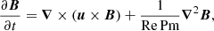
In this scaling scheme, the equations governing the evolution of the fluid velocity u, the magnetic field B, and the temperature perturbations T′ (around the background adiabatic state) are: the momentum equation

the induction equation
and the evolution equation for the temperature perturbations
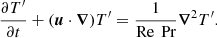
The flow and the magnetic field obey to the continuity conditions

The four dimensionless control parameters of the problem are: the Reynolds number

the ratio of the reference Brunt–Väisälä frequency N to the reference rotation rate Ωa,
the Prandtl number

and the magnetic Prandtl number

In this work we fix the aspect ratio of the spherical shell χ = ri/ro to 0.3. We employ stress-free boundary conditions for the flow. Electrically insulating boundary conditions are assumed for the magnetic field, which are appropriate to match a potential field outside the fluid volume.
The azimuthal body force
in Eq. (2) imposes the background axisymmetric differential rotation. Here  is the axisymmetric azimuthal velocity and uf = s Ωf is the forced contribution, which is axisymmetric (∂uf/∂ϕ = 0). The timescale τ in Eq. (10) provides the time on which
  relaxes to uf and is fixed to 5 × 10⁻³. This is the shortest timescale in the system and practically sets the numerical integration time step in our simulations.
The forced angular velocity Ωf is vertically invariant and is defined by
where μ = Ωe/Ωa < 1. Here Ωe is the angular velocity at the equator on the outer boundary. The real constant b > 0 defines the steepness of the decay of Ωf with the cylindrical radius s. In this work we consider μ = 0.45 and b = 2.9. The black line in Fig. 1a shows Ωf as a function of the cylindrical radius s for this parameter combination. Figure 1b presents a snapshot of the axisymmetric angular velocity  in one of our numerical simulations and demonstrates that this closely follows the forced angular velocity Ωf.
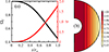 |
Fig. 1. Forced angular velocity employed in the simulations. (a) Forced angular velocity Ωf (Eq. (11) with μ = 0.45 and b = 2.9) and shear parameter q as a function of the cylindrical radius s/ro. (b) Snapshot of the axisymmetric angular velocity |

The forced angular velocity that we choose here simultaneously maximizes the mean and the maximum of the shear parameter q = |dlnΩf/dlns| in the fluid domain while still maintaining the flow stable according to the Rayleigh criterion for inviscid flows, which prescribes ∂L2/∂s > 0, where  is the specific AM. In the unstratified case, that is when 𝒩 = 0 and there is no temperature equation to solve, we verified numerically that this flow is indeed hydrodynamically stable to weak nonaxisymmetric perturbations by performing nonmagnetic runs at the typical Reynolds numbers Re explored here. The shear parameter q increases monotonically with s and attains its maximum value on the outer boundary at the equator where q ≈ 1.77 (Fig. 1a, red line). The mean value of q in the domain is 0.57. It is useful to define a characteristic timescale and length scale of the shear. The shear timescale is τΔΩ = ΔΩ−1, where ΔΩ = Ωa − Ωe = (1 − μ) Ωa ≈ Ωa/2 is the difference between the axial and the equatorial rotation rates. The shear length scale is
  , which can be estimated as
  .
.
The problem above is solved numerically using the open-source pseudospectral MHD code MagIC1 (Wicht 2002; Schaeffer 2013), which we modified to include the volumetric body force f in the momentum equation. The numerical technique is described in detail in Christensen & Wicht (2007) and we therefore mention only the essentials here. MagIC uses a poloidal-toroidal decomposition for the vector fields u and B and for the scalar temperature field. Spherical harmonics are employed in the latitudinal and azimuthal directions and Chebyshev polynomials in radius. An implicit-explicit time stepping scheme, where the nonlinear terms and the volumetric body force are treated explicitly, is employed. The nonaxisymmetric simulations performed here typically use a spatial resolution of 257 radial grid points and a maximum spherical harmonic (SH) degree ℓmax = 341. Depending on the characteristic scales of the turbulence to resolve, the spatial grid is sometimes coarser. The spherical harmonic kinetic and magnetic energy spectra of the solutions span at least three orders of magnitude in amplitude, which ensures numerical convergence of the results as we generally verified.
Throughout this work, we use the following notation for azimuthal, horizontal (over a spherical surface), and temporal averages of an arbitrary function f = f(r, θ, ϕ, t),
and
respectively. Here Δt is the time averaging period. In the following, only when explicitly specified, the angular brackets ⟨ ⋅ ⟩ denote spatial averages different from the one above. The nonaxisymmetric flow velocity and magnetic field are denoted by the superscript ′, for example  .
.
3. Unstratified axisymmetric solutions
We first describe the axisymmetric solutions obtained for an unstratified flow, that is when 𝒩 = 0 and there is no temperature equation to solve.
3.1. Initial magnetic field condition and dimensionless parameters
As initial condition for the magnetic field, we consider a purely azimuthal field linearly increasing with the cylindrical radius s,
where  is the field strength at s = 1. In differentially rotating radiative stellar interiors where a weak axisymmetric poloidal field
  is present, we expect dominantly azimuthal field configurations to be generated by the Ω-effect, that is by shearing the poloidal field through the differential rotation via the term
  in the azimuthal component of the axisymmetric induction equation (e.g., Spruit 1999). The azimuthal field would be stronger where the differential rotation is higher and, given our background angular velocity profile Ωf, this motivates the choice of the initial condition above.
To discuss the axisymmetric solutions, it is useful to rescale the magnetic field independently of the rotation rate by introducing the Hartmann number
The Hartmann number is related to the dimensionless parameters introduced in the previous section by Ha = Le Re Pm1/2 and can be interpreted as the ratio of the geometric mean of the viscous and magnetic diffusion times, τν = d2/ν and τη = d2/η respectively, to the Alfvén travel time d/uA. In the following Ha0 and Haϕ denote the Hartmann number based on the initial reference field strength  and on the azimuthal field
  respectively.
In Sect. 3.2 we discuss the flow and magnetic field solutions obtained when varying Ha0 and the Reynolds number Re at a fixed magnetic Prandtl number Pm of 1. For consistency with the new dimensionless magnetic field  , the flow velocity is scaled with d/(νη)1/2 and indicated with
  in this section.
3.2. Temporal evolution
The black lines in Fig. 2 illustrate the temporal evolution of the volume integrated magnetic energy  in four runs at Re = 5 × 10⁴ with Ha0 in the range 102 − 104 and in one run at the lower Re of 5 × 10³. Since no poloidal field is initialized, the solution remains purely toroidal. Axisymmetric magnetic fields cannot be maintained by dynamo action (Cowling’s antidynamo theorem) and the toroidal field decays exponentially due to Ohmic diffusion. The magnetic energy evolution is compatible with a field decay rate of
  , where
  is the characteristic azimuthal field length scale, which we calculated as a meridional average of
  at the last numerical integration time step of these runs (the gray line in Fig. 2 shows the exponential Ohmic decay rate of the run at Re = 5 × 10⁴ and Ha0 = 4 × 10³ as an example).
 |
Fig. 2. Temporal evolution of the magnetic energy Emag (black lines) and of the poloidal kinetic energy |


Due to the azimuthal flow forcing, the toroidal kinetic energy  , which is approximately 5.75 × 10⁹ and 5.75 × 10⁷ in the runs at Re = 5 × 10⁴ and 5 × 10³ respectively, is the dominant energy contribution and remains constant over time (not shown). Boundary driven flows produced by the Lorentz force induce a global meridional circulation in the first few rotation times τΩ, as evidenced by the initial rapid growth of the poloidal kinetic energy
  (red lines in Fig. 2). The peak amplitude of
  scales with
  and, on longer times,
  decays at a rate comparable to the one of the field, confirming the magnetic origin of the meridional flow. We now describe qualitatively how this global circulation is generated and how its morphology changes when varying Ha0.
The jump between the interior azimuthal field solution  and the electrically insulating boundary conditions, which impose
  at r = ri/d and ro/d, is accommodated in thin layers close to the boundaries, where the radial Lorentz force is strong due to the high radial gradients of the field. Due to the form of the interior field solution, the radial Lorentz force is stronger in the outer boundary layer than in the inner one. The Lorentz force in these boundary layers induces radial flows which, by mass conservation, generate return flows in the latitudinal direction. These return flows remain high in amplitude due to the stress-free boundary conditions and induce the large scale circulation observed. We note that the Lorentz force plays a similar dynamical role in modifying viscous boundary layers when a transverse magnetic field is applied (Hartmann boundary layers; see, e.g., Dormy & Soward 2007).
The boundary driven circulation is equatorially antisymmetric and, at the time when the poloidal kinetic energy peaks, is characterized by one cell in each hemisphere for the run at the lowest Ha0 of 102 (black isocontours in Fig. 3a). Increasing Ha0 to 103, the outer boundary layer thickness decreases as expected (black isocontours in Fig. 3b) and the meridional circulation amplitude strengthen (Fig. 2, dash double-dot red line). The radial Lorentz force is now important in the inner boundary layer as well, producing secondary circulation cells in the inner fluid regions (Fig. 3b). These secondary circulation cells are characterized by flows in the opposite direction to those of the primary ones, due to the opposite sign of the driving radial Lorentz force in the inner and outer boundary layers.
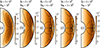 |
Fig. 3. Unstratified axisymmetric solutions of the runs in Fig. 2 at the times when the poloidal kinetic energy |

At Ha0 ≳ 4 × 10³, the circulation driven by the inner boundary layer extends toward the outer fluid regions and becomes comparable in amplitude to the outer one (black isocontours in Figs. 3c,e). The azimuthal field is efficiently advected by such strong flows and complex configurations with locally strong field gradients are produced (Figs. 3c,e).
Further evidence that the meridional flow in our simulations is of magnetic origin is given by the fact that the solution does not depend on Re. The evolution of the magnetic and kinetic energies of the two runs at Ha0 = 4 × 10³ in Fig. 2 with Re = 5 × 10³ (dotted-dashed line) and 5 × 10⁴ (dashed line) are indeed almost identical and snapshots of the two solutions are nearly indistinguishable (Figs. 3c,d). While the axisymmetric solutions above may be regarded as peculiar, they have to be considered only as initial states prone to AMRI. These solutions support turbulence for a period long enough to study the transport of AM and chemical elements, as we shall see in the following.
4. Linear stability
We now investigate the stability of the unstratified axisymmetric solutions discussed in the previous section. We introduce nonaxisymmetric perturbations after the magnetically driven meridional flows develop and the azimuthal field slowly decays due to Ohmic diffusion. The perturbations consist of a spatially uncorrelated random nonaxisymmetric toroidal field of weak amplitude. This is obtained by adding to the spherical harmonic decomposition of the toroidal field and for each radii small amplitude coefficients δhℓ, m(r) drawn from a uniform distribution for all degrees ℓ and orders m > 0. As in the previous section, the magnetic Prandtl number Pm is fixed to 1 here. The Reynolds number Re is varied in the range 103 − 105. At a fixed Re, to explore the effect of the background azimuthal field strength on the stability, we either perform runs with different Ha0 or we introduce the perturbations at successive times in a single run. The azimuthal field strength of the perturbed axisymmetric solution is characterized by the maximum value of Haϕ in the fluid domain at the perturbation time t = tpert. This is indicated as  hereafter and ranges from 60 to about 104.
4.1. Parameter space for stable and unstable regimes
Hydrodynamically stable shear flows with purely axisymmetric azimuthal fields as those considered here are stable to axisymmetric perturbations (Velikhov 1959), but they can be unstable to AMRI and to TI. At fixed Re, AMRI can develop only if the azimuthal field is nor too weak nor too strong, otherwise AMRI modes are stabilized by diffusive effects or by magnetic tension respectively. We provide order of magnitude estimates of these stability limits using results from the local linear stability analysis of Masada et al. (2006). The authors employ cylindrical coordinates and consider classical local harmonic perturbations with an azimuthal wavelength much larger than the meridional ones. The azimuthal velocity uϕ = sΩ and the toroidal field Bϕ of the basic, purely toroidal axisymmetric state are assumed to depend only on the cylindrical radius s. For an unstratified flow with strong differential rotation, as in most of our numerical simulations where  , the most unstable azimuthal mode predicted by the local linear analysis is
in the absence of diffusive effects. Here ωA = Bϕ/(μ0ρ)1/2s is the local azimuthal Alfvén frequency. The adiabatic growth rate of the most unstable mode is

AMRI can develop only when its most unstable mode grows faster than it decays by resistive effects (or equivalently by viscous effects since Pm = 1 here)
where  is the most unstable azimuthal wavenumber. Substituting Eqs. (14) and (15) in the relation above yields
when considering Ω ≈ Ωa, s ≈ d, and Pm = 1.
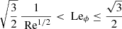
For increasing field strengths, large azimuthal modes are stabilized by magnetic tension and the spectrum of unstable modes shifts toward lower m. The condition  provides an upper limit on the field strength for instability which, for Pm = 1 and using the same values for Ω and s as above, reads
Combining Eqs. (17) and (18), we obtain the instability condition
when q < 4. For our simulations where q ≈ 1, Eq. (19) reduces to
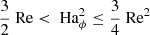
or equivalently
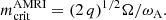
since Haϕ = Leϕ Re when Pm = 1. Another prediction from the local linear theory of Masada et al. (2006) that will be used in the following is the critical AMRI mode
As mentioned above, the axisymmetric solutions explored here are in principle unstable to both AMRI and TI. However, in the AMRI regime defined by Eq. (21), the expected most unstable TI mode is virtually always growing slower than the corresponding AMRI mode. The most unstable TI mode is  and its adiabatic growth rate, in the presence of rotation, is
  (Pitts & Tayler 1985; Spruit 1999; Bonanno & Urpin 2013). AMRI dominates over TI when
  , that is
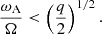
When assuming Ω ≈ Ωa, s ≈ d, and q ≈ 1 as done above, this condition reads

which is slightly smaller than the upper bound of Eq. (21). Similarly to what we obtain here using simple order of magnitude estimates, Jouve et al. (2015) showed that TI dominates over AMRI when Leϕ ≳ 1 by applying a local linear dispersion relation to dominant azimuthal field configurations obtained from direct numerical simulations.
Figure 4 compares our numerical simulation results with the predictions from the local linear analysis just discussed. Crosses show runs where the applied nonaxisymmetric perturbations decay and no instability is found; for circles and squares, the perturbations grow exponentially over time. Runs where, as demonstrated in the next section, we observe AMRI (orange symbols) fall within the region of the parameter space predicted by the instability condition Eq. (20) (white background) as expected. For low azimuthal field strengths 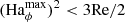 (gray background on the left) where AMRI is stabilized by diffusive effects according to the estimates above, we found no unstable run.
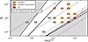 |
Fig. 4. Instability domain of the unstratified (𝒩 = 0) axisymmetric solutions at Pm = 1 and comparison with local and global linear stability analysis results. The Reynolds number Re is shown as a function of |


For larger azimuthal field strengths 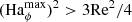 (gray background on the right), AMRI is expected to be suppressed by magnetic tension and we indeed observe TI (red circles). Evidence of TI in these simulation runs is provided in Appendix A. The critical
  of
of  for which the maximum TI growth rate becomes larger than the one of AMRI (red dotted line; cf. Eq. (24)) lies close to the boundary where AMRI is suppressed. In other words, in the AMRI regime, the maximum TI growth rate is virtually always lower than the one of AMRI.
Guseva et al. (2017b) performed a global linear stability analysis of AMRI in Taylor–Couette flow with a quasi-Keplerian shear that resembles the one employed here. The lower and upper neutral instability lines calculated by the authors (thick dashed lines in Fig. 4) agree remarkably well with our numerical simulation results.
In the reminder of this work, we focus on the AMRI regime only. In Sect. 5 we discuss the nonlinear evolution of the instability but we anticipate here that transient AMRI turbulence (orange circles in Fig. 4) is generally observed and only two runs at Re ≥ 5 × 10⁴ show self-sustained turbulence (orange squares).
4.2. Evidence of AMRI
We now analyze the linear evolution of the instability observed in our numerical simulations and provide evidence of AMRI. Here we focus on the run at Re = 5 × 10⁴ and  as an example. The perturbations are introduced at time tpert = 326.0. Similar results are obtained for the other unstable runs of Fig. 4 and we therefore do not discuss them in detail here.
Figures 5a,b present the initial temporal evolution of the toroidal and poloidal magnetic energies of various azimuthal modes m in this run. The energies are calculated over the spherical surface at radius r/ro = 0.9 and map the outer fluid regions where the instability first develops (Fig. 6a). As expected for AMRI, the instability fluctuations are larger in the outer equatorial region where the unstable modes have higher growth rates due to the stronger background shear (Fig. 1a).
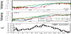 |
Fig. 5. Temporal evolution of various azimuthal modes and observed growth rates for the unstratified run at Re = 5 × 10⁴, |

Nonaxisymmetric azimuthal modes m < 25 grow exponentially typically after about 10 system rotations from the perturbation time until t − tpert ≈ 25 (Figs. 5a,b). The background axisymmetric (m = 0) azimuthal field (black line in Fig. 5a) slowly decays due to Ohmic diffusion and its evolution is practically stationary during the linear instability growth. We also observe the generation of an initially weak and decaying axisymmetric poloidal field (black line in Fig. 5b). This field is produced from weak nonlinear correlations of the initial flow and field instability fluctuations.
Figure 5c displays the growth rates of the nonaxisymmetric azimuthal modes m from 1 to 25, calculated from the evolution of the poloidal (dashed line) and toroidal (solid line) magnetic energies above during the period t − tpert = 9 − 24 of the linear instability growth. The two growth rates spectra are in good agreement between each other. According to the toroidal spectrum, modes m < 24 are linearly unstable. The most unstable mode is mmax = 14, although very similar growth rates are observed for the two adjacent modes m = 13 and 15. The longitudinal structure of the nonaxisymmetric azimuthal field  is compatible with such dominant modes (Fig. 6b).
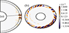 |
Fig. 6. Snapshot of the nonaxisymmetric azimuthal field |


The observed most unstable mode mmax and its growth rate γmax closely agree with the ones expected from the local linear theory discussed in the previous section. Equation (14) indeed provides  , which is very close to the observed most unstable mode. Here and in the remainder of this section the angular brackets ⟨ ⋅ ⟩ denote average over a spherical surface at radius r/ro = 0.9 where the azimuthal modes spectra above are calculated. Based on Eq. (15), the expected maximum growth rate of AMRI is
 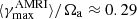 , which also closely agrees with the one observed from the toroidal spectrum at 0.30 (Fig. 5c).
The toroidal spectrum in Fig. 5c shows that the azimuthal modes m ≥ 24 are initially subcritical. This is again compatible with the local linear theory which predicts a critical azimuthal mode  (Eq. (22); red triangle in Fig. 5c). The linearly stable modes start to grow only at t − tpert ≳ 25 due to nonlinear mode energy transfers (the red line in Figs. 5a,b displays the evolution of m = 25 as an example), when we verified that the axisymmetric magnetic energy becomes comparable in amplitude to the nonaxisymmetric one. The nonlinear growth rates of the modes m = 1 and m = 2 (blue lines in Figs. 5a,b) are roughly twice the growth rate of mmax, possibly because of mode interactions between the faster growing linear modes. Finally, the instability saturates at t − tpert ≈ 55 with the nonaxisymmetric poloidal and toroidal energies roughly in equipartition.
Figure 7 displays the observed maximum growth rates γmax and the most unstable azimuthal modes mmax for some of the unstable runs of Fig. 4 in the AMRI regime. The simulation data points are shown as a function of ⟨ωA/Ω⟩ at the perturbation time. The numerical results are in good agreement with the local linear analysis predictions for AMRI (Eqs. (15) and (14)), which are indicated by the gray shaded regions. The largest differences between the numerical and theoretical values are of about 20% in the maximum growth rate and of a factor 2 in the most unstable mode. Such differences are surprisingly very limited considering all the simplifying assumptions of the local linear analysis, which can only roughly describe the global modes excited in our numerical simulations.
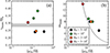 |
Fig. 7. Comparison of the observed most unstable AMRI modes and their growth rates with the local linear theory predictions. (a) Maximum growth rates γmax and (b) most unstable azimuthal modes mmax as a function of ⟨ωA/Ω⟩. The AMRI runs shown are those of Fig. 4 at |
5. Nonlinear solutions
In this section we discuss the nonlinear evolution of AMRI and describe the turbulent solutions obtained for unstratified and stratified flows. First, we consider the unstratified runs at Pm = 1 of the previous section. In Sect. 5.1 we describe in detail the fiducial dynamo run at Re = 5 × 10⁴ and  and we examine the dynamo onset in Sect. 5.2. The effect of Pm on the dynamo onset is presented in Sect. 5.3. Finally, Sect. 5.4 analyzes the nonlinear solutions obtained when including stable stratification.
5.1. Fiducial dynamo run
We describe the self-sustained turbulent solution of run U0 at 𝒩 = 0, Re = 5 × 10⁴, Pm = 1, and  , which we refer to as the fiducial dynamo run hereafter. The linear phase of the instability growth in this run has been discussed in Sect. 4.2.
Figure 8 presents the temporal evolution of the various components of the kinetic and magnetic energies. The dominant (stationary) toroidal axisymmetric kinetic energy of the background flow is  (not shown) and has been subtracted from the total kinetic energy contribution. After around 700 system rotations from the perturbation time tpert = 326.0, a stationary regime is reached. The magnetic energy of this state is dominantly nonaxisymmetric (dashed black line). The axisymmetric toroidal magnetic energy (dot dashed black line) is the second largest contribution, with an amplitude about 3 times smaller than the total magnetic energy. The axisymmetric poloidal field
  , generated by the instability fluctuations through the azimuthal component of the mean electromotive force (EMF)
  , is decisively weaker and saturates at an energy (dotted black line) roughly 2 orders of magnitude lower than the one of the axisymmetric toroidal field. Although weak, a positive EMF feedback on
  as the one observed here is crucial for MRI dynamos to operate. The Ω-effect obtained by shearing this weak
  through the background differential rotation provides indeed the required closure for self-sustained dynamo action (Rincon et al. 2007; Rincon 2019). The time averaged nonaxisymmetric magnetic energy of the steady state is about 4 times larger than the kinetic one (dashed red line). Similar turbulent magnetic to kinetic energy ratios are observed in global and local simulations of MRI turbulence with zero net flux (Reboul-Salze et al. 2021).
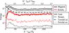 |
Fig. 8. Temporal evolution of the kinetic (red lines) and magnetic (black lines) energies for the fiducial dynamo run U0 (𝒩 = 0, Re = 5 × 10⁴, Pm = 1, and |

Figure 9 illustrates the complex turbulent character of the solution in the steady state. The magnetic field is small scaled in the meridional directions, while it presents elongated structures in the azimuthal direction, which are typical of MRI turbulence and are due to shear effects (Figs. 9a,b). Inside the tangent cylinder, the imaginary vertical cylindrical surface tangent to the inner boundary at the equator, the magnetic field is weak since AMRI is less active due to the low background shear (Fig. 1). Nonetheless, these regions host large scale axisymmetric poloidal fields confined at high latitudes by the meridional flow (black isocontours in Figs. 9c,d). Outside the tangent cylinder, both  and
and  are concentrated in small flux patches generated by the instability fluctuations (Fig. 9d). The structures of the flow velocity components are similar to those of the magnetic field, except for ur where the large scale meridional circulation produces radial plumes (Fig. 9c).
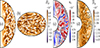 |
Fig. 9. Steady flow and magnetic field solution of the fiducial dynamo run U0 at time ts = 1241 (or ts − tpert = 915). (a,b) Meridional cut and surface projection at r/ro = 0.8 of the azimuthal field Bϕ. (c,d) Meridional cuts of the radial flow velocity ur and of the axisymmetric azimuthal field |

Dynamo action occurs when the magnetic field is sustained for a period longer than its characteristic Ohmic diffusion time  , where lB is a characteristic magnetic field length scale. Since the typical radial and latitudinal length scales of the magnetic field in the stationary state are similar, we estimate lB based on the horizontal length scales only. To this end, we define the instantaneous horizontal half wavelength of the field

where
is the mean SH degree of the field (Christensen & Aubert 2006). Here Bℓ, m is the coefficient at degree ℓ and order m of the SH expansion of the field and the angular brackets denote a volume integral over the fluid domain. The time average of lB, ⊥ during the steady state of the fiducial dynamo run is  , which yields an Ohmic diffusion time
  . The top horizontal axis of Fig. 8 shows that the quasi steady evolution of this run, which we define to start after about
  from the perturbation time, covers 1.84 τOhm and therefore self-sustained dynamo action is at work.
Hereafter we classify a simulation run as a dynamo if its quasi steady evolution lasts longer than τOhm. The simulation run presented here is the first MRI dynamo at a value of the magnetic Prandtl number Pm as low as 1 ever reported in a global setup. Previous global numerical studies have shown self-sustained MRI turbulence only for Pm ≥ 10 (Guseva et al. 2017b; Reboul-Salze et al. 2021). We remind here that these solutions have to be interpreted as small-scale dynamos, in the sense that the generated flow and magnetic fields are at scales smaller than the forcing scale of the background flow, which is on the order of ro in our runs (e.g., Rincon 2019).
Similarly to the above, we define the horizontal half wavelength of the flow lu, ⊥ = π d/ℓu, where ℓu is the mean SH degree of |u−uf|, the flow velocity amplitude after subtracting the contribution of the forcing. For the simplicity of notation, we refer to lu, ⊥ and lB, ⊥ as their time averaged values over a period of stationary evolution of the solution hereafter. For run U0, lu, ⊥ = 0.19 d, which is slightly larger than lB, ⊥. These horizontal length scales are listed, together with the control parameters and other output measures, in Table 1 for run U0 and for the other unstratified dynamos and stratified runs that we shall discuss in the next sections.
Input parameters and output diagnostics of the unstratified (𝒩 = 0) dynamo runs and of the stratified (𝒩 > 0) runs.
5.2. Dynamo onset at Pm = 1
Dynamo action driven by MRI is an inherently nonlinear phenomenon: it requires instability fluctuations that transiently grow to finite amplitudes, leading to nonlinear effects that eventually sustain the turbulence (Rincon et al. 2008). Linear MRI modes can easily reach finite amplitudes since they exhibit nonmodal growth, that is they can transiently grow faster than the least stable eigenmode on short timescales (e.g., Balbus & Hawley 1992; Squire & Bhattacharjee 2014; Mamatsashvili et al. 2020). Nonmodal effects are a well known property of non-self-adjoint linear systems, which include not only those prone to MRI but also purely hydrodynamical shear flows (Schmid 2007).
As a consequence of their nonmodal character, the excitation of MRI dynamos strongly depends on the amplitude and morphology of the initial condition (Riols et al. 2013; Guseva et al. 2017a). Consistently with these findings, as anticipated in Sect. 4.1, we observe self-sustained dynamo action in our unstratified simulations at Pm = 1 and fixed Re only when the field strength of the perturbed axisymmetric solution is large enough. Figure 10a compares the temporal evolution of the magnetic energy Emag, scaled as in Sect. 3, of the fiducial dynamo run U0 (solid black line) with two runs at lower  . The latter runs show transient turbulence where the instability decays after saturating for a period which shortens when
  decreases.
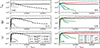 |
Fig. 10. Temporal evolution of the (a,b) magnetic energy Emag, the (c,d) turbulent magnetic Reynolds number Rm′, and the (e,f) turbulent Lundquist number Lu′ for six unstratified runs at Pm = 1. The solid black line shows the fiducial dynamo run U0. The left (right) panels present runs at Re = 5 × 10⁴ ( |


The turbulent magnetic Reynolds number

and the turbulent Lundquist number
where  and
and  are the root mean square (rms) nonaxisymmetric flow and magnetic field strengths respectively, can be used to compare the amplitudes of the flow and field instability fluctuations between these runs. The peak values reached by Rm′ and Lu′ increase with
  (Figs. 10c,e), arguably producing a stronger mean EMF
  which sustains the axisymmetric field against resistive effects at the larger
  of 5012 of run U0. As already mentioned above, this instability-driven EMF is key to generate the axisymmetric poloidal field required for MRI dynamos to operate. We note that studies of AMRI in Taylor–Couette flow also show that both the turbulent flow and field amplitudes increase with the imposed background field strength as we observe here (Rüdiger et al. 2013).
As anticipated in Sect. 4.1, we find dynamo action for Re ≥ 5 × 10⁴, that is when the azimuthal flow forcing is strong enough. Figure 10b indeed demonstrates that Emag in runs at a fixed  of 5012 decays for Re ≤ 2 × 10⁴, while a quasi steady state is reached in the two other runs at larger Re. The peak amplitudes of Rm′ and Lu′ increase with the Reynolds number (Figs. 10d,f), which again suggests that dynamo action occurs when the mean EMF becomes strong enough. The background differential rotation contrast from pole to equator ΔΩ scales roughly as Re/2 (Sect. 2). This produces a stronger Ω-effect in the two runs at larger Re which also helps to sustain the axisymmetric azimuthal field
  .
.
We remark here that the perturbed axisymmetric azimuthal field solutions of these runs at fixed  are very similar but not exactly identical. Although mild, these differences may contribute to explain the regime change from decaying to self-sustained turbulence when increasing Re. The critical magnetic Reynolds number for the onset of MRI dynamo action indeed strongly depends on the initial condition itself (Riols et al. 2013).
5.3. Dependence of the dynamo onset on Pm
Local shearing box simulations with zero or nonzero net magnetic fluxes show that viscous and resistive effects strongly affect the saturated state of MRI turbulence (Lesur & Longaretti 2007; Fromang et al. 2007; Simon & Hawley 2009). In particular, magnetic diffusion limits the turbulence saturation level such that, at fixed Re, dynamo action is lost below a critical value of Pm, a behavior that we also find here.
Figure 11 presents the temporal evolution of the nonaxisymmetric kinetic and magnetic energies in run U0 (black lines) and in two other runs at the same Re of 5 × 10⁴, but with Pm = 0.5 and 2 (run U1). After a few hundreds of system rotations, run U1 (green lines) reaches a quasi steady state covering a period Δt = 0.82 τOhm (Table 1). Given that the various energy components are stationary and that the period of quasi steady evolution is close to one Ohmic diffusion time, we consider this run as a dynamo. The time averaged turbulent kinetic and magnetic energies in the quasi steady state increase by about a factor 2 relative to run U0, in qualitative agreement with the shearing box studies mentioned above.
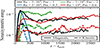 |
Fig. 11. Temporal evolution of the nonaxisymmetric kinetic (dashed lines) and magnetic (solid lines) energies for four unstratified runs at Re = 5 × 10⁴ and Re = 105 and different values of Pm as indicated in the legend at the top. The black lines show the fiducial dynamo run U0. |
When decreasing Pm to 0.5, AMRI turbulence is maintained only for some tens of system rotations and then it decays away (blue lines in Fig. 11). We note that the perturbed axisymmetric azimuthal field configurations of these runs are different, but their mean strength increases when Pm lowers which, in principle, favors dynamo action as discussed in the previous section. While this cannot justify the observed dynamo behavior, it may explain the large peak values of the turbulent energies reached by the nondynamo run at Pm = 0.5, which are comparable to those of runs U0 and U1.
The shearing box MRI studies mentioned above also indicate that the critical Pm for dynamo onset decreases when Re increases (e.g., Fromang et al. 2007). At the largest Re of 105 that we explored here, we indeed observe dynamo action for a value of Pm as low as 0.6 (run U3; red lines in Fig. 11). After an initial transient of about 340 system rotations the turbulence reaches a quasi steady evolution lasting for 1.6 τOhm. MRI dynamos at Pm < 1 are reported in local shearing box simulations with net magnetic fluxes (Simon & Hawley 2009; Käpylä & Korpi 2011), but never so far in global setups as the one explored here.
5.4. Effect of stable stratification on AMRI turbulence
We now study how stable stratification modifies unstratified AMRI turbulence at Re = 5 × 10⁴ and Pm = 1. To this end, we solve Eqs. (2)–(4) using as initial condition the quasi steady solution of the fiducial dynamo run U0 at time ts = 1241 (Fig. 9).
We first discuss the effect of stable stratification by varying 𝒩 at a fixed Prandtl number Pr of 10−3. Stable stratification strongly limits radial motions, modifying the characteristics of the turbulence. Figures 12a,b present the temporal evolution, starting at t = ts, of the turbulent (nonaxisymmetric) magnetic and kinetic energies in run U0 (black lines) and in the three stratified runs S0 (𝒩 = 1), S4 (𝒩 = 10), and S9 (𝒩 = 20), showing that they lower when increasing stratification. After an initial transient which gets longer when increasing 𝒩, the quasi steady evolutions of runs S4 (green lines) and S9 (red lines) cover 0.95 and 0.19 τOhm respectively. The turbulence in the weakly stratified run S0 (blue lines) slowly decays following the resistive decay of the background axisymmetric field (blue lines in Fig. 12c). By limiting radial motions, stable stratification lowers the effective magnetic Reynolds number  below the critical value for dynamo onset, which is of about 820 based on the unstratified simulations (Table 1). Here urms = (V−1∫|u−uf|2dV)1/2 is the rms flow velocity after subtracting the forced azimuthal flow. The energies of all stratified runs explored here display an oscillatory behavior (see the inset in Fig. 12a) which is characteristic of stratified MRI turbulence and is often attributed to an αΩ-dynamo process (Gressel 2010; Reboul-Salze et al. 2022).
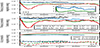 |
Fig. 12. Temporal evolution of the magnetic and kinetic energies of four unstratified and stratified runs at Re = 5 × 10⁴ and Pm = 1. (a) Nonaxisymmetric magnetic energy, (b) nonaxisymmetric kinetic energy, (c) axisymmetric toroidal (solid lines) and poloidal (dashed lines) magnetic energies as a function of time for the unstratified fiducial dynamo run U0 (black) and the three runs S0, S4, and S9 at 𝒩 = 1, 10, and 20 respectively (see the legend in the middle panel). All the stratified runs are at Pr = 10−3. The inset in (a) shows the nonaxisymmetric magnetic energies of runs S0 and S4 on a linear scale. The initial condition of the stratified runs is the steady state solution of run U0 at time ts = 1241 shown in Fig. 9. |
The location and structure of the turbulence also change with stratification. The snapshots of  in Figs. 13d–f reveal that the turbulence in the weakly stratified run S0 remains homogeneous outside the tangent cylinder as in the unstratified fiducial dynamo, while the instability is confined up to intermediate latitudes in run S4 and is almost entirely located in the southern hemisphere in the most stratified run S9. The unstable regions in the two latter runs correlate with the locations where the axisymmetric azimuthal field
  is stronger (Figs. 13h,i) and unstable to AMRI according to the local linear analysis, which predicts
  based on the instability condition Eq. (21). Outside these locations,
  is too weak, with typical absolute amplitudes of 10−3 or smaller, and AMRI modes are damped by diffusive effects.
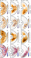 |
Fig. 13. Snapshots of the flow and magnetic field solutions of runs S0, S4, and S9 shown in Fig. 12. From top to bottom: meridional cuts of the azimuthal field Bϕ, nonaxisymmetric azimuthal field |


In the most stratified run S9, the turbulence becomes weakly anisotropic, with structures elongated in the latitudinal direction as expected (Fig. 13f). The horizontal turbulent field length scale  is 0.12 in this run, which is 60% larger than the value of the weakly stratified run S0 (Table 1). In the latitudinal direction, the structures of the flow are less stretched than those of the field, as evidenced by comparing the snapshots of Bϕ (Fig. 13c) and ur (Fig. 13l). The horizontal field length scale lB, ⊥/d is indeed as large as 0.76, whereas the one of the flow is lower at lu, ⊥/d = 0.27.
It is interesting to note that the axisymmetric toroidal magnetic energy increases with stratification (solid lines in Fig. 12c). This energy contribution dominates over the nonaxisymmetric one for 𝒩 > 1, so that Bϕ is characterized by larger spatial scales as stratification increases (Figs. 13a–c). On the contrary, the axisymmetric poloidal magnetic energy weakly lowers with stratification (dashed lines in Fig. 12c). As a consequence, the ratio  , where
  (
( ) is the time averaged rms axisymmetric azimuthal (poloidal) field, increases when increasing 𝒩 and ranges between 10 and 25 in our stratified simulations (Table 2). In the mean induction equation, the source terms that generate the axisymmetric toroidal field
  are the radial mean EMF
  and the term associated to the Ω-effect,
  , where
  is the axisymmetric poloidal field. In runs S4 and S9,
  is mostly concentrated in large flux patches located where the turbulence is most active which suggests a positive feedback of
  on its generation. The more coherent structure of the turbulence obtained when increasing stratification may yield locally stronger
  , which then causes the observed increase in
  . Although
  is weak in all runs explored, the Ω-effect – a key ingredient of MRI dynamos as mentioned before – is still of leading order due to the strong background shear. The positive feedback of the Ω-effect on the generation of
  is suggested, for example, by the positive flux patch in the northern hemisphere observed in run S9 (Fig. 13i). The maximum of this flux patch is indeed located where
  (black isocontours in Fig. 13i) is roughly antiparallel to the shear direction
  as expected.
The ratio of the time averaged rms azimuthal field to the radial one Bϕ, rms/Br, rms ranges between 3 and 5 in the unstratified and weakly stratified runs at 𝒩 = 1 and increases when stable stratification strengthens. At Pr = 10−3, for example, Bϕ, rms/Br, rms grows from 4.1 to 14.8 when increasing 𝒩 from 1 to 20. This field ratio is in the range 2 − 6 in global compressible simulations of stratified MRI turbulence in accretion disks (Hawley et al. 2011, 2013), while local shearing box simulations obtain values around 2 (Shi et al. 2010).
By reducing the amplitude of the temperature fluctuations, thermal diffusion can weaken the stabilizing buoyancy force in Eq. (2). This occurs when thermal diffusion acts faster than the buoyancy force, that is when τκ < τN, where  is the thermal diffusion timescale at the radial flow length scale lr and τN = 1/N is the buoyancy timescale. By equating these two timescales, we obtain the critical (radial) flow length scale lc = (κ/N)1/2, or lc/d = (Pr Re 𝒩)−1/2, below which thermal diffusion weakens buoyancy. To explore the effect of thermal diffusion in our stratified simulations at Re = 5 × 10⁴ and Pm = 1, we varied the Prandtl number Pr at fixed 𝒩.
Figure 14a displays the temporal evolution of the turbulent magnetic energy (solid lines) in four runs at 𝒩 = 10 with Pr increasing from 10−4 to 10−2. While AMRI is observed for Pr ≤ 2 × 10⁻³, further increasing the Prandtl number to 10−2 (solid red line) suppresses the instability. In this stable run the nonaxisymmetric modes decay at a rate increasing with the azimuthal wavenumber m as expected (Fig. 14b).
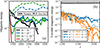 |
Fig. 14. Effect of the Prandtl number Pr on the instability. (a) Nonaxisymmetric (solid lines) and axisymmetric toroidal (dashed lines) magnetic energies as a function of time in runs S3–S6 (Re = 5 × 10⁴, Pm = 1, 𝒩 = 10, and different values of Pr as indicated in the legend). Only the nonaxisymmetric energy is shown for run S6 at Pr = 10−2. (b) Toroidal magnetic energy at radius r/ro = 0.5 as a function of time for the azimuthal modes m = 0 − 6 for the stable run S6. |
The analysis of a few snapshots of the turbulent radial velocity  shows that the radial flow length scale lr, obtained from a volume average of
  , is ≲O(lc) for Pr ≤ 2 × 10⁻³, which suggests that buoyancy effects are limited by thermal diffusion in these runs. In the run at Pr = 10−2, on the contrary, lr/d ≈ 0.05 is several times larger than the critical length scale lc/d = 0.014, hence thermal diffusion cannot reduce the effect of stable stratification, which is too strong and suppresses the instability. Similarly, we observe AMRI turbulence at 𝒩 = 20 when Pr ≤ 10−3, whereas the instability is suppressed at the larger Pr of 5 × 10⁻³ (Table 1). A similar behavior where increasing buoyancy effects stabilizes the system is also typical of hydrodynamical shear instabilities in vertically stratified flow (Lignières et al. 1999). We remark here that strong enough latitudinal gradients of the differential rotation allow AMRI to develop even when lc ≪ lr and thermal diffusion does not limit stable stratification (Jouve et al. 2020).
Finally, we note that all stratified AMRI runs show either transient turbulence or cover periods too short to test for dynamo action. For example, at 𝒩 = 10, we found decaying turbulence at Pr = 10−4 (Fig. 14a, solid black line). The decay rate of the turbulent fluctuations is compatible with the one of the axisymmetric azimuthal field which sustains the instability (Fig. 14a, dashed black line). In the two runs at Pr = 10−3 and 2 × 10⁻³, the turbulence is sustained for 0.19 and 0.09 Ohmic diffusion times τOhm respectively and it may decay on longer timescales not captured here (Table 1). These periods correspond to, respectively, 140 and 115 eddy turnover times τeddy, which ensure a robust statistics for the turbulence. Hereafter τeddy is defined as the time averaged ratio  .
.
6. Angular momentum transport
In this section we examine the transport of AM induced by AMRI in the unstratified and stratified simulations described above. An equation of conservation for the specific AM  can be obtained by averaging the azimuthal component of Eq. (2) over longitude and multiplying both members by s = r sin θ,

where

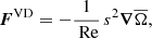
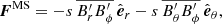
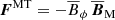
are the fluxes of the meridional circulation (MC), Reynolds stresses (RS), viscous diffusion (VD), Maxwell stresses (MS), and magnetic tension (MT) respectively. Hereafter the subscript M indicates the meridional component (e.g., 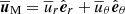 ). Note that there is no contribution from the magnetic pressure B2/2 in Eq. (29) since the longitudinal magnetic pressure gradient vanishes when integrated over ϕ.
We decompose the flux terms Eqs. (30)–(34) into the sum of their radial and latitudinal contributions, that is
where i = {MC, RS, VD, MS, MT}; for example, the Reynolds stresses flux is  , where
  and
and  . To assess the net AM transport in the radial and latitudinal directions, following Brun & Toomre (2002), we integrate
  and
and  over spherical surfaces of varying radii and over cones of varying inclination respectively,
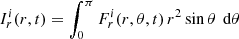
and
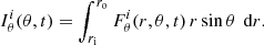
We then time average these integrated fluxes, obtaining  and
and  respectively. In the unstratified dynamo runs, the time averages are calculated over quasi steady states generally covering intervals Δt of a few hundreds of eddy turnover times τeddy (Table 1). In the stratified runs the turbulence is transient and no steady state is reached, so that the time averaging interval Δt is defined by periods, after the initial transient, where the turbulent magnetic energy does not decay significantly. Such periods cover at least 56 τeddy (Table 1), which still ensures a robust statistics for the turbulence.
6.1. Unstratified dynamo runs
First, we analyze the AM transport in the unstratified dynamo runs described in Sects. 5.1–5.3. Figures 15a,d present the time averaged integrated fluxes  and
and  in the fiducial dynamo run U0. In both directions, the Maxwell stresses (red lines) and meridional circulation (black lines) fluxes largely dominate over all the other contributions. In the radial direction, the third largest contribution is the Reynolds stresses flux
  (green line in Fig. 15a) with a peak amplitude more than 4 times lower than the one of the Maxwell stresses flux
  . Viscous diffusion and magnetic tension come next, with peak amplitudes of
  and
and  about 10 and 30 times smaller than the one of
  . In the latitudinal direction, the Reynolds stresses, viscous diffusion and magnetic tension fluxes all have comparable amplitudes and, similarly to the radial fluxes, their peak values are one order of magnitude lower than
  .
.
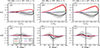 |
Fig. 15. Time averaged integrated fluxes (a–c) |


The color shaded areas in Figs. 15a,d show the 1 standard deviation intervals around the time averaged fluxes and evidence that the temporal variability of the meridional circulation fluxes is much higher than the one of all the other terms. This high variability is due to an oscillatory behavior of the meridional flow (dotted red line in Fig. 8) where the dominant large scale meridional circulation cells characterizing the steady state solution (black isocontours in Fig. 9c) are regularly replaced by new ones of opposite sign. These new meridional circulation cells are generated by radial flow plumes arising at mid and high latitudes in the inner fluid regions.
Since the radial fluxes of the prevailing Maxwell stresses and meridional circulation dominate over the respective latitudinal contributions, the transport of AM mainly occurs in the radial direction. The Maxwell stresses transport AM radially outward since  . The meridional circulation contributes to the outward transport in the internal fluid regions where r/ro ≲ 0.6, while it opposes in the external regions at larger radii (black line in Fig. 15a). It is not surprising that the meridional flow contributes to the radial transport. In fact, the radial length scales of the meridional circulation cells are comparable to the characteristic scale of the background shear lΔΩ ≈ ro (Fig. 9c, black isocontours).
The larger amplitudes of  with respect to
  suggest a net outward AM transport. This is confirmed by an additional numerical experiment that we performed by stopping the forcing (f = 0) during the quasi steady evolution of run U0 and letting the azimuthal flow free to evolve. We observe the cylindrical rotation profile flattening over time, with the azimuthal flow decelerating in the interior and accelerating in the equatorial region to reach uniform rotation on a few hundreds of rotation times τΩ (Appendix B).
Although negligible relative to the radial one, the transport of AM in the latitudinal direction is also dominated by the Maxwell stresses and the meridional circulation. The former produce an equatorward transport since  is equatorially antisymmetric, with a positive (negative) contribution in the northern (southern) hemisphere (Fig. 15d, red line).
  is mostly positive (Fig. 15d, black line), hence it contributes to the equatorward transport by the Maxwell stresses in the northern hemisphere and it opposes in the southern one. The amplitudes of
  are generally comparable to the one of
  , except in the equatorial region and at low latitudes in the southern hemisphere where the former is larger.
We now discuss how the transport varies with Re and Pm. The middle and right panels of Fig. 15 display the time averaged integrated fluxes of the dynamo runs U2 and U1 respectively, which we discussed in Sects. 5.2 and 5.3. Relative to the fiducial dynamo run U0, run U2 has a larger Re of 105 and run U1 a larger Pm of 2. Similarly to the fiducial dynamo, the radial transport in these runs dominates over the latitudinal one and we therefore discuss only the former in the following (Figs. 15b,c,e,f). The net transport occurs radially outward due to the prevailing radial Maxwell stresses (Fig. 15b). The peak amplitudes of  in runs U2 and U1 are, respectively, about 3 and 2 times higher than the one of run U0, which suggest similar variations in the AM transport efficiency. The time averaged rms turbulent field strenghts
  of runs U2 and U1 are 50% and 41% larger than the one of run U0 respectively, which contributes to explain the observed variations in the Maxwell stresses flux (Table 2). The time averaged rms turbulent flow velocity
  in these runs is also a few tens of percent higher than the one of run U0 and contribute to explain the increase of the radial Reynolds stresses flux
  (green lines in Figs. 15b,c).
Similarly to run U0, the meridional circulation in runs U2 and U1 opposes the radial transport by the Maxwell stresses over most of the fluid domain (black lines in Figs. 15b,c). The meridional circulation in these runs is still large scaled and its rms amplitude  is about 20% higher than the one of run U0 (Table 2), which can explain the observed variations of
  . These faster meridional flows may result from the higher Reynolds and Maxwell stresses which contribute to the meridional circulation maintenance (see, e.g., Miesch 2005). Likewise to run U0, viscous diffusion and magnetic tension play a negligible role in the transport. Similar variations of the flux contributions with Pm are obtained at Re = 105 by comparing run U2 with run U3 at Pm = 0.6 (not shown).
The weaker dependence of the Reynolds and Maxwell stresses on Pm than on Re that we just discussed qualitatively agrees with previous results obtained from local and global simulations of unstratified MRI turbulence. Guseva et al. (2017b) showed that the transport coefficient, the sum of the Reynolds and Maxwell stresses, of AMRI turbulence in Taylor–Couette flow scales as Pm1/2Re when Rm ≳ 102. Local shearing box simulations with zero net flux suggest a similar scaling with Pm, although the variation with Re is much weaker than the linear one obtained for Taylor–Couette flow (Lesur & Longaretti 2007).
6.2. Stably stratified runs
By weakening radial motions, stable stratification modifies the transport of AM. Here we discuss how the transport varies with stratification considering the three runs S0, S4, and S9 (Pr = 10−3 and 𝒩 = 1, 10, and 20 respectively) discussed in Sect. 5.4. Figure 16 displays the time averaged integrated fluxes  and
and  in these runs, together with the fiducial dynamo run U0 in the two leftmost panels for the sake of reference. In the weakly stratified run S0, the transport occurs similarly to the unstratified case. Only a small decrease of the dominant Maxwell stresses and meridional circulation fluxes is observed (red and black lines in Figs. 16b,f). However, the meridional circulation shows a much weaker variability, as demonstrated by the small 1 standard deviation intervals around
  and
and  (gray shaded regions in Figs. 16b,f), since the oscillatory behavior observed for run U0 is absent.
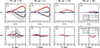 |
Fig. 16. Same as Fig. 15 but for the three stratified runs S0, S4, and S9 at Pr = 10−3 and 𝒩 = 1, 10, and 20 respectively (second to fourth from left panels). The leftmost panels show the unstratified fiducial dynamo run U0 for the sake of comparison. All runs are at Re = 5 × 10⁴ and Pm = 1. |
Increasing 𝒩 to 10 (run S4) produces a sizeable decrease of the radial Maxwell stresses flux  (red line in Fig. 16c). The latitudinal Maxwell stresses flux
  is confined at low to intermediate latitudes (red line in Fig. 16g), which correlates with the locations where the instability is active (Fig. 13e). The transport by the meridional flow becomes almost negligible (black lines in Figs. 16c,g) since radial flow motions are severely limited by the stabilizing buoyancy force. The meridional flow amplitude
  is indeed 2.5 times smaller than the one of the weakly stratified run S0 (Table 2) and multiple meridional circulation cells elongated in the latitudinal direction are observed (black isocontours in Fig. 13k). The horizontal flow length scale lu, ⊥/d increases to 0.22, while is smaller at 0.17 in run S0 as expected.
In run S9 at 𝒩 = 20,  further weakens and its peak amplitude becomes comparable to the respective latitudinal contribution
  (red lines in Figs. 16d,h). The latitudinal Maxwell stresses flux is concentrated in the southern hemisphere at the locations where the axisymmetric azimuthal field is strong enough to support AMRI (Sect. 5.4). The transport by the meridional circulation remains very weak as in run S4 (black lines in Figs. 16d,h) and no significant variation in the meridional flow amplitude is observed (Table 2). However, the meridional circulation cells become thinner in the radial direction as expected (black isocontours in Fig. 13l).
Similar results on the variation of the integrated fluxes are obtained when strengthening buoyancy effects by reducing thermal diffusion, that is when increasing Pr at fixed 𝒩. Since the Maxwell stresses dominate the transport, we discuss only their variation with Pr here. Figure 17 presents  and
and  in runs S3, S4, and S5 at 𝒩 = 10 and Pr = 10−4, 10−3, and 2 × 10⁻³ respectively. Similarly to the runs discussed above, the radial Maxwell stresses flux prevails over the latitudinal one. The amplitude of
  lowers when Pr increases and its distribution shifts toward the outer fluid regions where the instability is active (Fig. 17a). Similarly to what has been observed above for run S9,
  concentrates in the southern hemisphere when buoyancy effects are stronger at the larger Pr of 2 × 10⁻³ (green line in Fig. 17b).
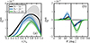 |
Fig. 17. Time averaged integrated (a) radial and (b) latitudinal Maxwell stresses fluxes in runs S3, S4, and S5, which are at Pr = 10−4, 10−3, and 2 × 10⁻³ respectively. The other parameters are Re = 5 × 10⁴, Pm = 1, and 𝒩 = 10. The shaded areas show 1 standard deviation above and below the time averages. |
In all stratified runs explored here, Reynolds stresses, viscous diffusion and magnetic tension contribute very weakly to the AM transport in both the radial and latitudinal directions. Magnetic tension is the weakest of all contributions since  is always small as we discussed in Sect. 5.4.
6.3. Turbulent viscosity
We demonstrated above that the AM transport induced by AMRI occurs radially outward and is dominated by the Maxwell stresses when 𝒩 > 1. The meridional circulation contribution is significant only in the unstratified and weakly stratified runs at 𝒩 = 1. To quantify the transport efficiency, we therefore consider the contribution by the radial Maxwell stresses only and we assume the classical turbulent viscosity hypothesis in which AM is transported in the direction of slow rotation,
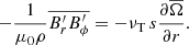
Here νT is the radial turbulent viscosity and  . We obtain the turbulent viscosity estimate
  from the relation above by taking first a volume average of both members,
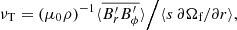
and then by time averaging Eq. (39) over the intervals Δt defined before and listed in Table 1. In runs showing transient turbulence,  has to be interpreted as an upper estimate for the transport efficiency since the instability decays on timescales longer than Δt. The dimensionless turbulent viscosity estimate is
 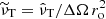 , where we employed the shear timescale τΔΩ = ΔΩ−1 and the shear length scale lΔΩ ≈ ro as reference scales.
Figure 18 displays  as a function of 𝒩 for all unstable runs at Re = 5 × 10⁴ and Pm = 1 explored here. The turbulent viscosity lowers when buoyancy effects strengthen, that is when 𝒩 and/or Pr increase. The largest value of
  is 3.7 × 10⁻⁴ and is obtained for the unstratified fiducial dynamo run U0 as expected (black circle). In the stratified runs at 𝒩 > 1, the turbulent viscosity approaches the unstratified value when Pr decreases since thermal diffusion limits the stabilizing buoyancy force. In the weakly stratified runs at 𝒩 = 1 the effect of stable stratification on the radial Maxwell stresses is only marginal (Sect. 6.2) and therefore
  shows only a weak decrease relative to the unstratified run.
 |
Fig. 18. Turbulent viscosity |


At fixed Prandtl number Pr, the turbulent viscosity  lowers when increasing 𝒩. At Pr = 10−3, for example,
  varies by roughly a factor 6 in the range of stratification explored. When 𝒩 increases from 1 (run S0) to 10 (run S4), such variation is mostly due to changes in the turbulent field amplitudes. In fact,
  decreases by more than a factor 2 from run S0 to run S4 and (
 )2 lowers by a factor 1.6 (Table 2). The residual turbulent viscosity variation may be an effect of volume averaging. The unstable fluid regions of run S4 are indeed more localized than those of run S0, as already discussed in Sect. 5.4. This is also clearly evidenced by the distribution of
  , the time averaged radial Maxwell stresses flux, which is shown in Figs. 19b,c for these two runs. The smaller turbulent viscosity value of run S9 at 𝒩 = 20 instead originates from the weaker spatial correlations of the turbulence, together with a volume averaging effect. In fact, runs S9 and S4 share a similar value of
  of 0.018 (Table 2) but the peak amplitudes of
  are 40% lower in the former run (Figs. 19c,d).
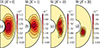 |
Fig. 19. Time averaged radial Maxwell stresses fluxes |

The variations of  with Pr, observed when 𝒩 > 1 is fixed, likewise originate from changes in both the size of the unstable regions and the spatial correlations of the turbulent field. In these runs, while
  weakly changes with Pr (Table 2), the integrated Maxwell stresses flux
  reduces when Pr increases (Sect. 6.2), which suggests a decrease of the spatial correlations of the turbulent field. The distribution of
  also narrows as Pr increases, which yields smaller values for the volume averaged Maxwell stresses in our turbulent viscosity estimate.
A power law of the form  , where δ > 0, well describes the dependence of the turbulent viscosity on stratification. A least squares fit of the runs at Pr = 10−3 provides an exponent δ = 0.50 and a prefactor a = 3.1 × 10⁻⁴ (dashed line in Fig. 18). For AMRI turbulence in Taylor–Couette flow, Spada et al. (2016) suggest a stronger scaling of 𝒩−1. For a free shear, Jouve et al. (2020) demonstrated that some of the linear properties of AMRI, such as the instability threshold and the range of linearly unstable modes, depend only on the parameter combination 𝒩2Pr. However, our simulations indicate that this is not the case for the nonlinear evolution of AMRI and for the AM transport efficiency.
7. Transport of chemical elements
7.1. Model formulation
We assume the light stellar chemical elements to contaminate the turbulent fluid flow as a passive scalar, that is their concentration is so low that they have no dynamical influence on the fluid motion itself. The equation of evolution of the chemical concentration c is
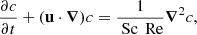
which is solved together with Eqs. (2)–(4). Here the Schmidt number

is the ratio of the fluid kinematic viscosity ν to the molecular chemical diffusivity Dc. We consider Sc = 1 so that the diffusion timescale of the chemicals d2/Dc and the viscous timescale of the flow τν = d2/ν are equal. We assume no sources nor sinks of the chemical elements from the boundaries by imposing a zero chemical concentration flux ∂c/∂r = 0 at r = ri and ro. The initial distribution of the chemical concentration is the spherically symmetric Gaussian
![$$ \begin{aligned} c(r, t=t_0) = \frac{1}{C_0}\exp \left[{-\frac{(r-r_0)^2}{2\sigma _0^2}}\right]. \end{aligned} $$](/articles/aa/full_html/2024/03/aa47672-23/aa47672-23-eq244.gif)
The distribution is centered at mid depth in the fluid domain, r0 = (1/χ−1)−1 + 1/2, and has a full width at half maximum of δ0/d = 1/10, which corresponds to a variance  . The total mass of the chemicals in the fluid domain C0 = ∫c(t = t0) dV is a conserved quantity and serves as a normalization constant here.
The chemical layer Eq. (42) is introduced during the turbulent AMRI evolution of the unstratified fiducial dynamo run U0 and of all the stratified runs at the times t = t0 listed in Table 3. In the following sections we study the turbulent transport of the chemicals, we estimate its efficiency and we compare the results with the AM transport.
Input parameters and output diagnostics of the simulations where a passive scalar is introduced.
7.2. Estimate of the turbulent chemical diffusivity
First, we examine the temporal evolution of the azimuthally averaged (mean) chemical concentration  in our numerical simulations and analyze the turbulent transport. If the turbulent transport occurs as a diffusive process, the radial distribution of
  remains Gaussian over time and its variance σ2 increases linearly. The rate at which σ2 grows defines the radial turbulent chemical diffusivity

In all runs explored here, the turbulent transport of the mean chemical concentration is diffusive during the initial stages of its evolution. Figure 20a displays the evolution of the radial profile of the horizontally averaged mean chemical concentration  in run C5 (𝒩 = 10 and Pr = 10−3) as an example. The distribution remains Gaussian for a period of about
  after t0 and its variance σ2 increases linearly as expected (Fig. 20c; see also the snapshots of
  in Figs. 21a–c). We calculated the turbulent chemical diffusivity DT from Eq. (43) by performing a time average of dσ2/dt over this interval (dashed line in Fig. 20c), which covers 12 eddy turnover times τeddy (see the upper horizontal axis of Fig. 20c). This procedure yields a dimensionless chemical diffusivity
  of 5.4 × 10⁻⁵. The last column of Table 3 reports the estimates
  for all runs explored here.
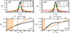 |
Fig. 20. Chemical turbulent transport for run C5 at 𝒩 = 10 and Pr = 10−3 (left panels) and for the unstratified run C0 (right panels). (a,b) Radial distribution of the horizontally averaged mean chemical concentration |


In run C5, deviations from a diffusive transport begin at time t − t0 ≈ 200 when σ2 starts to level off and does not evolve linearly anymore (Fig. 20c). At t − t0 = 400 the distribution of the mean concentration becomes decisively non-Gaussian and its flanks reach the boundaries (Fig. 20a, red line). A snapshot of  at this time evidences that the meridional circulation contributes, on such longer timescales, to expel the chemicals from the central parts of the fluid domain, accumulating them at high latitudes in the southern hemisphere (Fig. 21d). We estimated a characteristic timescale for the meridional flow in the region of the chemical layer as
  , where
  is the horizontally averaged meridional velocity at t = t0. In run C5
  (vertical dotted line in Fig. 20c), which agrees well with the timescale on which σ2 starts to deviate from the initial diffusive evolution.
 |
Fig. 21. Snapshots of the mean chemical concentration |


When buoyancy effects weaken by considering lower 𝒩 and/or Pr, the meridional flow timescale τM decreases as expected (Table 3) and therefore the transport of the chemicals by the meridional flow takes over the turbulent one earlier during the evolution. Nonetheless, the shortest period of diffusive evolution in our stratified simulations, obtained for run C1 (𝒩 = 1 and Pr = 10−3), covers about 8 τeddy, which still ensures a robust statistics for the turbulence.
In the unstratified run C0 the diffusive phase covers an even shorter interval of 3.7 τeddy (orange shaded area in Fig. 20d). The meridional flow timescale τM reduces to  and
and  becomes decisively non-Gaussian already at t − t0 = 70 (Fig. 20b, red line; Fig. 21h). The estimate of
  in run C0 is therefore less accurate than all the other runs where a reliable measurement is instead achieved. In this run the standard deviation of
  is as large as 31% of the turbulent diffusivity value itself. In the runs at 𝒩 = 10 and 20 and higher Pr, the standard deviation is instead of only a few percent of
  since the diffusive phase lasts more than 10 τeddy (Table 3). For a diffusive transport, a certain degree of scale separation between the initial chemical layer width δ0 and the characteristic radial length scale of the turbulence is required. While in runs at 𝒩 > 1 such a scale separation is verified, in run C0 this becomes only marginally satisfied, as evidenced by the strong latitudinal variations of
  (Figs. 21f,g), and may cause additional accuracy loss in our estimate of the turbulent diffusivity.
7.3. Chemical and angular momentum transport
We now discuss how the efficiency of the chemical turbulent transport varies with the effect of stratification. Figure 22a shows that  lowers when buoyancy effects strengthen either by increasing 𝒩 and/or Pr. The two most weakly stratified runs at 𝒩 = 1 with Pr = 10−3 and 10−2 have values of
  comparable to the unstratified case (black circle) within their 1 standard deviation intervals. In the runs at 𝒩 = 10 and 20, as discussed in the previous section, the turbulent diffusivity estimates become more accurate due to the longer diffusion phase and the uncertainties are generally smaller than the symbol sizes themselves. As with the turbulent viscosity, a power law well describes the dependence of the chemical diffusivity on stratification. A power law fit of the stratified runs at Pr = 10−3 provides
  (dashed line in Fig. 22a). The exponent of 𝒩 is very similar to the one obtained for the turbulent viscosity (Sect. 6.3).
 |
Fig. 22. Efficiency of the turbulent transport of the chemicals and comparison with the one of angular momentum. (a) Turbulent chemical diffusivity |


The turbulent Schmidt number

measures the efficiency of the AM transport relative to the one of the chemical elements. Figure 22b displays ScT as a function of 𝒩 for all simulation runs and shows that this is always larger than 1 and does not vary much with increasing buoyancy effects in the ranges of 𝒩 and Pr explored. The value ScT = 1.96 ± 0.75 of the unstratified run C0 (black circle) encompasses all the other estimates obtained for the stratified runs, except for the case at 𝒩 = 1 and Pr = 10−1 which is larger at ScT = 3.8. Our simulations therefore suggest that AMRI turbulence induces a transport of AM which is systematically stronger than the one of chemical elements. This is expected since the Maxwell stresses, which dominate the transport of AM in our runs and do not directly influence the one of chemical elements, are generally stronger than the Reynolds stresses (Sects. 6.1 and 6.2), which instead regulate the chemical transport. However, we note that  , the ratio of the volume averaged radial Maxwell stresses to the volume averaged radial Reynolds stresses, is always larger than 5 (Table 2) and overestimates the relative transport efficiency measured by ScT.
8. Summary and discussion
Additional transport processes beyond atomic diffusion and standard hydrodynamical mechanisms, such as meridional circulation and shear turbulence, are required to explain the observed rotational and chemical evolution of low-mass stars. MHD turbulence is regarded as one of the primary processes to enhance the transport in radiative stellar interiors. In this work we investigated numerically the transport of AM and chemical elements due to azimuthal MRI in a spherical shell where cylindrical differential rotation is forced.
We first considered an unstratified flow at a magnetic Prandtl number Pm of 1 and explored the stability of purely axisymmetric toroidal field configurations to weak nonaxisymmetric perturbations. The parameter regime where we observe AMRI agrees well with predictions obtained from a local linear stability analysis and with the global linear analysis results of Guseva et al. (2017b) who analyze Taylor–Couette flow with an imposed field. Our AMRI runs are characterized by values of  not smaller than about 5 × 10⁻³, otherwise diffusive effects stabilize the system, and not larger than about 0.5, or else the nature of the instability changes and TI is found. Here
  is the maximum value in the fluid domain of the ratio of the Alfvén frequency of the axisymmetric azimuthal field
  to the reference rotation rate Ωa.
Next, we explored the nonlinear evolution of the instability in these unstratified runs. At Pm = 1, we observe self-sustained dynamo action when Re ≥ 5 × 10⁴ and the azimuthal field strength of the perturbed axisymmetric solution is large enough (runs U0 and U2). At the larger Re of 105, we find dynamo action down to Pm = 0.6 (run U3). These simulations are the first global MRI dynamos ever reported at such low values of Pm. We obtain transient turbulence in all the other unstable runs.
We then examined the effect of thermal stable stratification on unstratified AMRI turbulence at Re = 5 × 10⁴ and Pm = 1. To this end, we varied 𝒩 = N/Ωa, the ratio of the Brunt–Väisälä frequency to the reference rotation rate, from 1 to 20 and the Prandtl number Pr in the range 10−4 − 10−1. When increasing buoyancy effects, the turbulence becomes less isotropic and homogeneous. However, when Pr is too large, thermal diffusion cannot limit the stabilizing buoyancy force anymore and AMRI is suppressed. In our most stratified unstable runs, we observe instability structures elongated in the latitudinal direction and unstable regions localized in the southern hemisphere where the axisymmetric azimuthal field is strong enough to support AMRI. All the stratified runs show transient turbulence, although in a few cases the numerical integration time is too short to test for dynamo action. We argue that, by limiting radial flow motions, stable stratification reduces the effective magnetic Reynolds number Rmeff below the critical value for dynamo onset, which is of about 800 based on the unstratified runs. Nonetheless, the magnetic and kinetic energies show an oscillatory behavior typical of αΩ-dynamos that has been reported before (e.g., Reboul-Salze et al. 2022).
We explored the transport of AM in the unstratified dynamo solutions and in the stratified runs, showing that it occurs radially outward and is largely dominated by the Maxwell stresses when 𝒩 ≥ 10. The meridional circulation opposes to the radial transport by the Maxwell stresses only when no stratification is present or is weak at 𝒩 = 1. We quantified the radial AM transport by estimating the turbulent viscosity  , where ΔΩ is the global rotation contrast and ro the outer boundary radius, and we show that it decreases when buoyancy effects strengthen. Within the explored range of parameters, the turbulent viscosity variations are well described by the power law
  , where a = 3.1 × 10⁻⁴.
Finally, we investigated the turbulent transport of a passive scalar. After demonstrating that this occurs as a diffusive process, we estimated the diffusion coefficient  . In the range of parameters explored,
  varies with buoyancy effects similarly to the turbulent viscosity
  but its magnitude is sistematically lower. A power law
  well describes our simulation data so that the turbulent Schmidt number
  is always of about 2 in the range of parameters explored. When buoyancy effects are high enough and the AM transport is dominated by the turbulent magnetic field fluctuations and the one of the chemicals by the flow fluctuations, we tested whether the ratio of the radial Maxwell stresses to the radial Reynolds stresses is a good proxy for ScT. We find that this ratio generally overestimates ScT by roughly a factor 3 in our simulations.
As far as an application to stars is concerned, there are several limitations to the setup explored here. First, we examined MRI of purely toroidal fields whereas magnetic field configurations with both toroidal and poloidal components are expected in stellar interiors. Secondly, the background differential rotation profile and its amplitude may not be representative of the shear in stellar interiors. We also ignored the additional stabilizing effect of chemical buoyancy in the momentum equation. Relaxing one or more of these assumptions may yield to turbulent diffusion coefficients that differ from those estimated here.
However, other fluid properties employed in our simulations approach those expected in certain regions of stellar interiors. For example, the values of the molecular diffusivity ratios and of the stable stratification are close to those of the electron-degenerate cores of red giants and of the nondegenerate radiative outer regions of these stars, respectively. In fact, the Prandtl number Pr is typically ∼10−3 in degenerate red giant cores (Garaud et al. 2015) and the magnetic Prandtl number Pm ranges between 10−1 and 10 (Rüdiger et al. 2015). The nondegenerate radiative regions immediately above the hydrogen burning shell are less dense than the degenerate zones below and expand during their evolution, hence the thermal component of the Brunt–Väisälä frequency NT is relatively low at ∼10−3 s−1 in the subgiant phase and further decreases to about 5 × 10⁻⁴ s−1 on the red giant branch (Talon & Charbonnel 2008). The typical angular rotation frequency Ω/2π of the cores of these stars is roughly in the range 600 − 700 nHz (Deheuvels et al. 2014; Gehan et al. 2018), which yields NT/Ω ≈ 100 − 200, that is only from 5 to 10 times larger than the highest value of 𝒩 = 20 employed in our simulations. Such moderate values of NT/Ω also charaterize the interior of pre-MS stars (Gouhier et al. 2021).
However, in both the radiative regions of red giants above and below the hydrogen burning shell, the values of the molecular diffusivity ratios and NT/Ω cannot be captured simultaneously. In the degenerate cores, NT/Ω is as large as ∼103 during the subgiant phase and increases to 104 in evolved red giants (Talon & Charbonnel 2008). In the outer nondegenerate layers, where the diffusivities are dominated by radiative and collisional contributions only, Pr and Pm drop to about 10−7 and 10−2 respectively (Garaud et al. 2015; Rüdiger et al. 2015).
We show that the turbulent viscosity in our simulations scales with 𝒩−1/2, which is slower than the 𝒩−1 scaling suggested for AMRI in Taylor–Couette flow with imposed current-free magnetic fields (Spada et al. 2016). Assuming that our scaling prediction  is confirmed for larger values of the stable stratification than those explored here, we obtain a turbulent viscosity
  in the range 2 − 7 × 108 cm2 s−1 for the degenerate cores of subgiants and red giants. For 𝒩, here we used the values of NT/Ω discussed above; for the shear contrast ΔΩ/2π we considered the typical angular velocity difference between the core and the envelope of subgiants of 900 nHz, and for the radius of the radiative region ro = 0.05 R⊙, which is 2% of the typical radius of subgiants R = 2.5 R⊙ (Deheuvels et al. 2014). Such a high turbulent viscosity value enforces solid body rotation in the degenerate core on a timescale of around 2000 yr, which is not incompatible with the observations. It is indeed likely that the observed radial shear of subgiants is localized around the hydrogen burning shell, hence above the degenerate core which may be in rigid rotation instead (Deheuvels et al. 2014). This observational evidence is further supported by the fact that stable stratification peaks at the hydrogen burning shell, where the transport of AM would be the slowest (Fuller et al. 2019). In regions around the hydrogen burning shell, chemical stratification largely dominates over the thermal contribution. The thermal Brunt–Väisälä frequency NT is lower in these regions than in the core so that our scaling predicts even larger turbulent viscosity values, hence faster transport than the one estimated above. Stellar evolution models that reproduce the rotational evolution of low-mass evolved stars suggest a significantly smaller turbulent diffusion coefficient which increases monotonically from 102 cm2 s−1 in early subgiants to almost 106 cm2 s−1 at the end of the red giant phase (Spada et al. 2016; Moyano et al. 2022).
Our simulations show that the transport of AM due to AMRI may be more efficient than the one induced by TI. The theory of Fuller et al. (2019) for TI-driven dynamo action predicts that the turbulent viscosity scales as (NT/Ω)−2, whereas here we obtain a power exponent of −1/2 for AMRI. TI dynamo action may have been recently identified in global numerical simulations (Petitdemange et al. 2023), but robustly testing the proposed turbulent viscosity scalings requires further study.
The magnetic field strengths recently measured in red giant cores can be directly compared to our numerical simulation results in terms of the radial Lenhert number  , the ratio of the local Alfvén frequency based on the rms radial field
  to the rotation rate Ω. In the 13 red giants where magnetic field measurements exist so far,
  ranges between 0.05 and 0.25 at the hydrogen burning shell, the region of maximum sensitivity for the asteroseismic inversions (Li et al. 2023). Such strong field amplitudes are incompatible with those expected from TI dynamo action which predicts
  , where N here is the Brunt–Väisälä frequency including both thermal and compositional contributions (Fuller et al. 2019; Li et al. 2022, 2023). For AMRI, our numerical results indicate that
  decreases less steeply with thermal stratification. However, the typical values we obtain at a moderate stratification of 𝒩 = 20 are
  , which is already one order of magnitude lower than the smallest observed value.
Although AMRI turbulence seems unable to explain the strong magnetic fields observed in the core, we cannot exclude that weaker fields could be generated in the outer radiative regions of red giants, in particular above the hydrogen burning shell where NT/Ω is lower at ∼102 as discussed before. AMRI could also be triggered during earlier stages of the evolution of low-mass stars, for example during the core contraction phase immediately after the main sequence. Numerical simulations suggest that large scale fields, relic of a core convective dynamo during the main sequence, can destabilize the differential rotation produced by core contraction through axisymmetric MRI (Gouhier et al. 2022).
Recent stellar evolution models indicate that MHD turbulence is required to reconcile the internal rotation of the Sun with its surface Li abundance and to reproduce the observed Li depletion of pre-main sequence and solar-type stars (Eggenberger et al. 2022). These models employ prescriptions for the transport by TI dynamo action where the turbulent Schmidt number scales as ScT ∼ (N/Ω)2 ≫ 1. We show that AMRI turbulence transports AM more efficiently than chemical elements, as suggested by these stellar evolution models, but ScT is too low at values of about 2 and does not show significant variations for the moderate degrees of thermal stratification explored.
In conclusion, we confirm that AMRI turbulence can strongly enhance the transport of AM and chemical elements in radiative stellar interiors and its efficiency may be higher than the one of TI. The turbulent viscosity moderately decreases with stable stratification and the chemical turbulent diffusion coefficient follows a similar scaling but is weaker in amplitude. While our numerical simulations capture the mild molecular diffusivity ratios of degenerate stellar cores, extensive parameter investigations are needed to robustly extrapolate the results at the extreme degrees of stratification that characterize stellar interiors. Further numerical studies in a spherical geometry exploring MRI-induced transport for different shear profiles and amplitudes than those examined here and considering chemical buoyancy could give additional insights on the rotational and chemical evolution of low-mass stars.
Acknowledgments
The authors acknowledge support from the project BEAMING ANR-18-CE31-0001 of the French National Research Agency (ANR). L.J. acknowledges support from the Institut Universitaire de France. This work was performed using high performance computing resources from CALMIP (Grants 2021A-P1118, 2021B-P1118, 2022A-P1118, 2022B-P1118 and 2023A-P1118) and from GENCI-IDRIS (Grants 2022-A0110410970 and 2023-AD0100413776). The authors are indebted to Sébastien Deheuvels and François Rincon for helpful discussions and thank an anonymous referee whose insightful comments have improved the quality of the manuscript.
References
- Aerts, C., Mathis, S., & Rogers, T. M. 2019, ARA&A, 57, 35 [Google Scholar]
- Arlt, R., Hollerbach, R., & Rüdiger, G. 2003, A&A, 401, 1087 [NASA ADS] [CrossRef] [EDP Sciences] [Google Scholar]
- Balbus, S. A., & Hawley, J. F. 1992, ApJ, 400, 610 [CrossRef] [Google Scholar]
- Beck, P. G., Bedding, T. R., Mosser, B., et al. 2011, Science, 332, 205 [Google Scholar]
- Bonanno, A., & Urpin, V. 2012, ApJ, 747, 137 [NASA ADS] [CrossRef] [Google Scholar]
- Bonanno, A., & Urpin, V. 2013, A&A, 552, A91 [NASA ADS] [CrossRef] [EDP Sciences] [Google Scholar]
- Brun, A. S., & Toomre, J. 2002, ApJ, 570, 865 [CrossRef] [Google Scholar]
- Cantiello, M., Mankovich, C., Bildsten, L., Christensen-Dalsgaard, J., & Paxton, B. 2014, ApJ, 788, 93 [Google Scholar]
- Charbonnel, C., Lagarde, N., Jasniewicz, G., et al. 2020, A&A, 633, A34 [NASA ADS] [CrossRef] [EDP Sciences] [Google Scholar]
- Christensen, U. R., & Aubert, J. 2006, Geophys. J. Int., 166, 97 [NASA ADS] [CrossRef] [Google Scholar]
- Christensen, U., & Wicht, J. 2007, Core Dynamics, (Elsevier) 8, 245 [NASA ADS] [Google Scholar]
- Deheuvels, S., Doğan, G., Goupil, M. J., et al. 2014, A&A, 564, A27 [NASA ADS] [CrossRef] [EDP Sciences] [Google Scholar]
- Deheuvels, S., Li, G., Ballot, J., & Lignières, F. 2023, A&A, 670, L16 [NASA ADS] [CrossRef] [EDP Sciences] [Google Scholar]
- Deliyannis, C. P. 2000, ASP Conf. Ser., 198, 235 [NASA ADS] [Google Scholar]
- Dormy, E., & Soward, A. M. 2007, Mathematical Aspects of Natural Dynamos (Chapman and Hall/CRC) [CrossRef] [Google Scholar]
- Dumont, T., Charbonnel, C., Palacios, A., & Borisov, S. 2021, A&A, 654, A46 [NASA ADS] [CrossRef] [EDP Sciences] [Google Scholar]
- Eggenberger, P., Montalbán, J., & Miglio, A. 2012, A&A, 544, L4 [NASA ADS] [CrossRef] [EDP Sciences] [Google Scholar]
- Eggenberger, P., den Hartogh, J. W., Buldgen, G., et al. 2019, A&A, 631, L6 [NASA ADS] [CrossRef] [EDP Sciences] [Google Scholar]
- Eggenberger, P., Buldgen, G., Salmon, S. J. A. J., et al. 2022, Nat. Astron., 6, 788 [NASA ADS] [CrossRef] [Google Scholar]
- Fromang, S., Papaloizou, J., Lesur, G., & Heinemann, T. 2007, A&A, 476, 1123 [NASA ADS] [CrossRef] [EDP Sciences] [Google Scholar]
- Fuller, J., Lecoanet, D., Cantiello, M., & Brown, B. 2014, ApJ, 796, 17 [Google Scholar]
- Fuller, J., Piro, A. L., & Jermyn, A. S. 2019, MNRAS, 485, 3661 [NASA ADS] [Google Scholar]
- Garaud, P., Medrano, M., Brown, J. M., Mankovich, C., & Moore, K. 2015, ApJ, 808, 89 [NASA ADS] [CrossRef] [Google Scholar]
- Gehan, C., Mosser, B., Michel, E., Samadi, R., & Kallinger, T. 2018, A&A, 616, A24 [NASA ADS] [CrossRef] [EDP Sciences] [Google Scholar]
- Goossens, M., & Tayler, R. J. 1980, MNRAS, 193, 833 [NASA ADS] [Google Scholar]
- Goossens, M., Biront, D., & Tayler, R. J. 1981, Ap&SS, 75, 521 [NASA ADS] [CrossRef] [Google Scholar]
- Gouhier, B., Lignières, F., & Jouve, L. 2021, A&A, 648, A109 [EDP Sciences] [Google Scholar]
- Gouhier, B., Jouve, L., & Lignières, F. 2022, A&A, 661, A119 [NASA ADS] [CrossRef] [EDP Sciences] [Google Scholar]
- Gressel, O. 2010, MNRAS, 405, 41 [NASA ADS] [CrossRef] [Google Scholar]
- Griffiths, A., Eggenberger, P., Meynet, G., Moyano, F., & Aloy, M.-Á. 2022, A&A, 665, A147 [NASA ADS] [CrossRef] [EDP Sciences] [Google Scholar]
- Guseva, A., Hollerbach, R., Willis, A. P., & Avila, M. 2017a, Phys. Rev. Lett., 119, 164501 [NASA ADS] [CrossRef] [Google Scholar]
- Guseva, A., Willis, A. P., Hollerbach, R., & Avila, M. 2017b, ApJ, 849, 92 [NASA ADS] [CrossRef] [Google Scholar]
- Hawley, J. F., Guan, X., & Krolik, J. H. 2011, ApJ, 738, 84 [NASA ADS] [CrossRef] [Google Scholar]
- Hawley, J. F., Richers, S. A., Guan, X., & Krolik, J. H. 2013, ApJ, 772, 102 [NASA ADS] [CrossRef] [Google Scholar]
- Hollerbach, R., Teeluck, V., & Rüdiger, G. 2010, Phys. Rev. Lett., 104, 044502 [NASA ADS] [CrossRef] [Google Scholar]
- Jouve, L., Gastine, T., & Lignières, F. 2015, A&A, 575, A106 [NASA ADS] [CrossRef] [EDP Sciences] [Google Scholar]
- Jouve, L., Lignières, F., & Gaurat, M. 2020, A&A, 641, A13 [EDP Sciences] [Google Scholar]
- Käpylä, P. J., & Korpi, M. J. 2011, MNRAS, 413, 901 [CrossRef] [Google Scholar]
- Kirillov, O. N., Stefani, F., & Fukumoto, Y. 2012, ApJ, 756, 83 [NASA ADS] [CrossRef] [Google Scholar]
- Lesur, G., & Longaretti, P. Y. 2007, MNRAS, 378, 1471 [NASA ADS] [CrossRef] [Google Scholar]
- Li, G., Deheuvels, S., Ballot, J., & Lignières, F. 2022, Nature, 610, 43 [NASA ADS] [CrossRef] [Google Scholar]
- Li, G., Deheuvels, S., Li, T., Ballot, J., & Lignières, F. 2023, A&A, 680, A26 [NASA ADS] [CrossRef] [EDP Sciences] [Google Scholar]
- Lignières, F., Califano, F., & Mangeney, A. 1999, A&A, 349, 1027 [NASA ADS] [Google Scholar]
- Lodders, K., Palme, H., & Gail, H. P. 2009, Landolt-Börnstein, New Series, 4B, 560 [Google Scholar]
- Mamatsashvili, G., Chagelishvili, G., Pessah, M. E., Stefani, F., & Bodo, G. 2020, ApJ, 904, 47 [NASA ADS] [CrossRef] [Google Scholar]
- Marques, J. P., Goupil, M. J., Lebreton, Y., et al. 2013, A&A, 549, A74 [NASA ADS] [CrossRef] [EDP Sciences] [Google Scholar]
- Masada, Y., Sano, T., & Takabe, H. 2006, ApJ, 447, 447 [NASA ADS] [CrossRef] [Google Scholar]
- Meduri, D. G., Lignières, F., & Jouve, L. 2019, Phys. Rev. E, 100, 013110 [NASA ADS] [CrossRef] [Google Scholar]
- Miesch, M. S. 2005, Liv. Rev. Sol. Phys., 2, 1 [Google Scholar]
- Moyano, F. D., Eggenberger, P., Meynet, G., et al. 2022, A&A, 663, A180 [NASA ADS] [CrossRef] [EDP Sciences] [Google Scholar]
- Moyano, F. D., Eggenberger, P., Mosser, B., & Spada, F. 2023, A&A, 673, A110 [NASA ADS] [CrossRef] [EDP Sciences] [Google Scholar]
- Ogilvie, G. I., & Pringle, J. E. 1996, MNRAS, 279, 152 [NASA ADS] [CrossRef] [Google Scholar]
- Petitdemange, L., Marcotte, F., & Gissinger, C. 2023, Science, 379, 300 [NASA ADS] [CrossRef] [Google Scholar]
- Pinçon, C., Belkacem, K., Goupil, M. J., & Marques, J. P. 2017, A&A, 605, A31 [NASA ADS] [CrossRef] [EDP Sciences] [Google Scholar]
- Pitts, E., & Tayler, R. J. 1985, MNRAS, 216, 139 [NASA ADS] [CrossRef] [Google Scholar]
- Reboul-Salze, A., Guilet, J., Raynaud, R., & Bugli, M. 2021, A&A, 645, A109 [NASA ADS] [CrossRef] [EDP Sciences] [Google Scholar]
- Reboul-Salze, A., Guilet, J., Raynaud, R., & Bugli, M. 2022, A&A, 667, A94 [NASA ADS] [CrossRef] [EDP Sciences] [Google Scholar]
- Rincon, F. 2019, J. Plasma Phys., 85, 205850401 [NASA ADS] [CrossRef] [Google Scholar]
- Rincon, F., Ogilvie, G. I., & Proctor, M. R. E. 2007, Phys. Rev. Lett., 98, 254502 [NASA ADS] [CrossRef] [Google Scholar]
- Rincon, F., Ogilvie, G. I., Proctor, M. R. E., & Cossu, C. 2008, Astron. Nachr., 329, 750 [NASA ADS] [CrossRef] [Google Scholar]
- Riols, A., Rincon, F., Cossu, C., et al. 2013, J. Fluid Mech., 731, 1 [NASA ADS] [CrossRef] [Google Scholar]
- Rüdiger, G., Hollerbach, R., Gellert, M., & Schultz, M. 2007, Astron. Nachr., 328, 1158 [CrossRef] [Google Scholar]
- Rüdiger, G., Gellert, M., Schultz, M., Hollerbach, R., & Stefani, F. 2013, MNRAS, 438, 271 [Google Scholar]
- Rüdiger, G., Gellert, M., Spada, F., & Tereshin, I. 2015, A&A, 573, A80 [NASA ADS] [CrossRef] [EDP Sciences] [Google Scholar]
- Schaeffer, N. 2013, Geochem. Geophys. Geosyst., 14, 751 [NASA ADS] [CrossRef] [Google Scholar]
- Schmid, P. J. 2007, Annu. Rev. Fluid Mech., 39, 129 [NASA ADS] [CrossRef] [Google Scholar]
- Shi, J., Krolik, J. H., & Hirose, S. 2010, ApJ, 708, 1716 [NASA ADS] [CrossRef] [Google Scholar]
- Simon, J. B., & Hawley, J. F. 2009, ApJ, 707, 833 [NASA ADS] [CrossRef] [Google Scholar]
- Spada, F., Gellert, M., Arlt, R., & Deheuvels, S. 2016, A&A, 589, A23 [NASA ADS] [CrossRef] [EDP Sciences] [Google Scholar]
- Spruit, H. C. 1999, A&A, 349, 189 [NASA ADS] [Google Scholar]
- Spruit, H. C. 2002, A&A, 381, 923 [CrossRef] [EDP Sciences] [Google Scholar]
- Squire, J., & Bhattacharjee, A. 2014, ApJ, 797, 67 [NASA ADS] [CrossRef] [Google Scholar]
- Talon, S., & Charbonnel, C. 2008, A&A, 482, 597 [NASA ADS] [CrossRef] [EDP Sciences] [Google Scholar]
- Tayler, R. J. 1973, MNRAS, 161, 365 [CrossRef] [Google Scholar]
- Velikhov, E. P. 1959, J. Exptl. Theoret. Phys., 36, 1398 [Google Scholar]
- Wheeler, J. C., Kagan, D., & Chatzopoulos, E. 2015, ApJ, 799, 85 [NASA ADS] [CrossRef] [Google Scholar]
- Wicht, J. 2002, Phys. Earth Planet. Int., 132, 281 [CrossRef] [Google Scholar]
Appendix A: Tayler instability
As mentioned in Sect. 4.1, we observe TI in two of our unstratified simulation runs at Pm = 1. Here we provide evidence of this instability in run U4 at Re = 5 × 10³ and  = 5012.
TI is a pinch-type instability of purely toroidal fields expected to occur in radiative stellar interiors (Tayler 1973; Spruit 1999). In spherical coordinates, Goossens & Tayler (1980) studied the adiabatic stability of weak axisymmetric toroidal fields Bϕ(r, θ) when no rotation is present using an energy method. The toroidal field Bϕ has arbitrary radial dependence and angular dependence (1 − x2)1/2dPℓ/dx, where x = cos θ and Pℓ is the Legendre polynomial of degree ℓ. The field is weak in the sense that the magnetic pressure is much smaller than the hydrostatic pressure, so that it does not modify the basic stellar equilibrium. A necessary and sufficient condition for nonaxisymmetric instability is (Goossens et al. 1981)
The instability is most likely for azimuthal modes |m| = 1 and for large latitudinal gradients of  . A Taylor expansion easily shows that the regions close to the poles (|x|≪1) are always unstable for |m| = 1. Away from the poles, instability can also occur but only if
  increases sufficiently rapidly with x. The growth rate of the most unstable mode
  is on the order of the toroidal Alfvén frequency
  (Tayler 1973; Goossens et al. 1981). Rotation has a stabilizing influence on TI. Although not removing the instability, it reduces its maximum growth rate to (Pitts & Tayler 1985; Bonanno & Urpin 2013)

Figure A.1 displays the temporal evolution of the toroidal and poloidal magnetic energies of the spherical harmonic orders 0 ≤ m ≤ 10 for run U4. The nonaxisymmetric perturbations grow exponentially after about 2 system rotations from the perturbation time tpert = 33.2. The most unstable azimuthal mode is m = 1 (solid purple lines) as expected for TI. Its linear growth rate is γmax/Ωa ≈ 1.9 and 1.6 when calculated over the time interval t − tpert = 2 − 4 of the rms toroidal and poloidal field evolutions respectively (cf. black dashed lines in Fig. A.1).
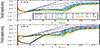 |
Fig. A.1. Temporal evolution of the (a) toroidal and (b) poloidal magnetic energies of the azimuthal modes m = 0 − 10 for run U4 (𝒩 = 0, Re = 5 × 10³, Pm = 1, and |

The instability saturates at t − tpert ≈ 12 when the rms nonaxisymmetric toroidal field strength is roughly 5 times lower than the one of the axisymmetric toroidal field  and about 2 times higher than the nonaxisymmetric poloidal one. We observe the generation of axisymmetric poloidal field
  due to the flow and field instability fluctuations at a rate which is roughly twice the one of the m = 1 mode (solid black line in Fig. A.1b). After saturation, the instability decays on longer times not shown in Fig. A.1.
During its linear growth, the instability is localized close to the poles, but also around the central equatorial regions of the fluid domain (Fig. A.2a,b). For the axisymmetric azimuthal field configuration  that we perturbed (Fig. A.2c), the instability condition (A.1) predicts, in addition to the classical wedge-shaped regions around the poles, several other unstable locations dispersed at lower latitudes, which originate from locally high latitudinal gradients of the field (gray shaded areas in Fig. A.2d). The unstable central equatorial regions correlate with the locations where the expected growth rates
  from Eq. (A.2) are larger (Fig. A.2d) and where the instability is also observed. At these locations
  , which agrees well with the growth rate γmax of the m = 1 mode observed in the simulation run.
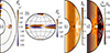 |
Fig. A.2. Tayler instability in run U4 and comparison with local linear analysis predictions. (a) Meridional cut and (b) surface projection of the nonaxisymmetric azimuthal field |


We also observe TI in the unstratified run at Re = 104 and  = 9787 (Fig. 4) and we obtain similar results in the analysis of the linear instability growth that we therefore do not discuss here.
Appendix B: Free azimuthal flow evolution of the fiducial dynamo run U0
Here we confirm that a net outward transport of AM is induced by AMRI, as already anticipated by the analysis of Sect. 6, performing a numerical experiment where the azimuthal flow is free to evolve.
Figure B.1 displays part of the temporal evolution of the axisymmetric toroidal kinetic energy in the quasi steady state of the unstratified fiducial dynamo run U0 (t − tpert < 915). At t − tpert = 915.0 (vertical dashed line), the azimuthal body force f in the momentum equation (2) is set to zero. The azimuthal flow relaxes to a state of uniform rotation in a few hundreds of rotation times τΩ = 1/Ωa. Figure B.2 demonstrates that the initial cylindrical profile of the azimuthally averaged angular velocity  flattens over time under the influence of AMRI. The flow decelerates in the interior and accelerates in the outer regions, producing a net outward transport of AM, and reaches a state of almost rigid rotation at t − tpert ≈ 1200.
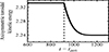 |
Fig. B.1. Axisymmetric toroidal kinetic energy as a function of time for the unstratified fiducial dynamo run U0 when the azimuthal flow is free to evolve. The azimuthal flow forcing is stopped (f = 0) at time t − tpert = 915.0 which is marked by the vertical dashed line. |
 |
Fig. B.2. Snapshots of the azimuthally averaged angular velocity |

All Tables
Input parameters and output diagnostics of the unstratified (𝒩 = 0) dynamo runs and of the stratified (𝒩 > 0) runs.
Input parameters and output diagnostics of the simulations where a passive scalar is introduced.
All Figures
|
Fig. 1. Forced angular velocity employed in the simulations. (a) Forced angular velocity Ωf (Eq. (11) with μ = 0.45 and b = 2.9) and shear parameter q as a function of the cylindrical radius s/ro. (b) Snapshot of the axisymmetric angular velocity |
| In the text | |
|
Fig. 2. Temporal evolution of the magnetic energy Emag (black lines) and of the poloidal kinetic energy |
| In the text | |
|
Fig. 3. Unstratified axisymmetric solutions of the runs in Fig. 2 at the times when the poloidal kinetic energy |
| In the text | |
|
Fig. 4. Instability domain of the unstratified (𝒩 = 0) axisymmetric solutions at Pm = 1 and comparison with local and global linear stability analysis results. The Reynolds number Re is shown as a function of |
| In the text | |
|
Fig. 5. Temporal evolution of various azimuthal modes and observed growth rates for the unstratified run at Re = 5 × 10⁴, |
| In the text | |
|
Fig. 6. Snapshot of the nonaxisymmetric azimuthal field |
| In the text | |
|
Fig. 7. Comparison of the observed most unstable AMRI modes and their growth rates with the local linear theory predictions. (a) Maximum growth rates γmax and (b) most unstable azimuthal modes mmax as a function of ⟨ωA/Ω⟩. The AMRI runs shown are those of Fig. 4 at |
| In the text | |
|
Fig. 8. Temporal evolution of the kinetic (red lines) and magnetic (black lines) energies for the fiducial dynamo run U0 (𝒩 = 0, Re = 5 × 10⁴, Pm = 1, and |
| In the text | |
|
Fig. 9. Steady flow and magnetic field solution of the fiducial dynamo run U0 at time ts = 1241 (or ts − tpert = 915). (a,b) Meridional cut and surface projection at r/ro = 0.8 of the azimuthal field Bϕ. (c,d) Meridional cuts of the radial flow velocity ur and of the axisymmetric azimuthal field |
| In the text | |
|
Fig. 10. Temporal evolution of the (a,b) magnetic energy Emag, the (c,d) turbulent magnetic Reynolds number Rm′, and the (e,f) turbulent Lundquist number Lu′ for six unstratified runs at Pm = 1. The solid black line shows the fiducial dynamo run U0. The left (right) panels present runs at Re = 5 × 10⁴ ( |
| In the text | |
|
Fig. 11. Temporal evolution of the nonaxisymmetric kinetic (dashed lines) and magnetic (solid lines) energies for four unstratified runs at Re = 5 × 10⁴ and Re = 105 and different values of Pm as indicated in the legend at the top. The black lines show the fiducial dynamo run U0. |
| In the text | |
|
Fig. 12. Temporal evolution of the magnetic and kinetic energies of four unstratified and stratified runs at Re = 5 × 10⁴ and Pm = 1. (a) Nonaxisymmetric magnetic energy, (b) nonaxisymmetric kinetic energy, (c) axisymmetric toroidal (solid lines) and poloidal (dashed lines) magnetic energies as a function of time for the unstratified fiducial dynamo run U0 (black) and the three runs S0, S4, and S9 at 𝒩 = 1, 10, and 20 respectively (see the legend in the middle panel). All the stratified runs are at Pr = 10−3. The inset in (a) shows the nonaxisymmetric magnetic energies of runs S0 and S4 on a linear scale. The initial condition of the stratified runs is the steady state solution of run U0 at time ts = 1241 shown in Fig. 9. |
| In the text | |
|
Fig. 13. Snapshots of the flow and magnetic field solutions of runs S0, S4, and S9 shown in Fig. 12. From top to bottom: meridional cuts of the azimuthal field Bϕ, nonaxisymmetric azimuthal field |
| In the text | |
|
Fig. 14. Effect of the Prandtl number Pr on the instability. (a) Nonaxisymmetric (solid lines) and axisymmetric toroidal (dashed lines) magnetic energies as a function of time in runs S3–S6 (Re = 5 × 10⁴, Pm = 1, 𝒩 = 10, and different values of Pr as indicated in the legend). Only the nonaxisymmetric energy is shown for run S6 at Pr = 10−2. (b) Toroidal magnetic energy at radius r/ro = 0.5 as a function of time for the azimuthal modes m = 0 − 6 for the stable run S6. |
| In the text | |
|
Fig. 15. Time averaged integrated fluxes (a–c) |
| In the text | |
|
Fig. 16. Same as Fig. 15 but for the three stratified runs S0, S4, and S9 at Pr = 10−3 and 𝒩 = 1, 10, and 20 respectively (second to fourth from left panels). The leftmost panels show the unstratified fiducial dynamo run U0 for the sake of comparison. All runs are at Re = 5 × 10⁴ and Pm = 1. |
| In the text | |
|
Fig. 17. Time averaged integrated (a) radial and (b) latitudinal Maxwell stresses fluxes in runs S3, S4, and S5, which are at Pr = 10−4, 10−3, and 2 × 10⁻³ respectively. The other parameters are Re = 5 × 10⁴, Pm = 1, and 𝒩 = 10. The shaded areas show 1 standard deviation above and below the time averages. |
| In the text | |
|
Fig. 18. Turbulent viscosity |
| In the text | |
|
Fig. 19. Time averaged radial Maxwell stresses fluxes |
| In the text | |
|
Fig. 20. Chemical turbulent transport for run C5 at 𝒩 = 10 and Pr = 10−3 (left panels) and for the unstratified run C0 (right panels). (a,b) Radial distribution of the horizontally averaged mean chemical concentration |
| In the text | |
|
Fig. 21. Snapshots of the mean chemical concentration |
| In the text | |
|
Fig. 22. Efficiency of the turbulent transport of the chemicals and comparison with the one of angular momentum. (a) Turbulent chemical diffusivity |
| In the text | |
|
Fig. A.1. Temporal evolution of the (a) toroidal and (b) poloidal magnetic energies of the azimuthal modes m = 0 − 10 for run U4 (𝒩 = 0, Re = 5 × 10³, Pm = 1, and |
| In the text | |
|
Fig. A.2. Tayler instability in run U4 and comparison with local linear analysis predictions. (a) Meridional cut and (b) surface projection of the nonaxisymmetric azimuthal field |
| In the text | |
|
Fig. B.1. Axisymmetric toroidal kinetic energy as a function of time for the unstratified fiducial dynamo run U0 when the azimuthal flow is free to evolve. The azimuthal flow forcing is stopped (f = 0) at time t − tpert = 915.0 which is marked by the vertical dashed line. |
| In the text | |
|
Fig. B.2. Snapshots of the azimuthally averaged angular velocity |
| In the text | |
Current usage metrics show cumulative count of Article Views (full-text article views including HTML views, PDF and ePub downloads, according to the available data) and Abstracts Views on Vision4Press platform.
Data correspond to usage on the plateform after 2015. The current usage metrics is available 48-96 hours after online publication and is updated daily on week days.
Initial download of the metrics may take a while.