| Issue |
A&A
Volume 630, October 2019
|
|
|---|---|---|
| Article Number | A149 | |
| Number of page(s) | 19 | |
| Section | Cosmology (including clusters of galaxies) | |
| DOI | https://doi.org/10.1051/0004-6361/201834485 | |
| Published online | 10 October 2019 | |
Secondary CMB anisotropies from magnetized haloes
I. Power spectra of the Faraday rotation angle and conversion rate
1
Institut d’Astrophysique Spatiale, UMR8617, CNRS, Univ. Paris-Sud, Univ. Paris-Saclay, Bâtiment 121, 91405 Orsay, France
e-mail: This email address is being protected from spambots. You need JavaScript enabled to view it.
2
Centro de Estudios de Física del Cosmos de Aragón (CEFCA), Plaza de San Juan, 1, Planta 2, 44001 Teruel, Spain
3
Département de Physique Théorique and Center for Astroparticle Physics, Université de Genève, 24 quai Ernest Ansermet, 1211 Geneva, Switzerland
4
Jet Propulsion Laboratory, California Institute of Technology, 4800 Oak Grove Drive, Pasadena, CA, USA
Received:
22
October
2018
Accepted:
14
May
2019
Abstract
Magnetized plasmas within haloes of galaxies leave their footprint on the polarized anisotropies of the cosmic microwave background. The two dominant effects of astrophysical haloes are Faraday rotation, which generates rotation of the plane of linear polarization, and Faraday conversion, which induces a leakage from linear polarization to circular polarization. We revisit these sources of secondary anisotropies by computing the angular power spectra of the Faraday rotation angle and the Faraday conversion rate by the large-scale structures. To this end, we use the halo model and we pay special attention to the impact of magnetic field projections. Assuming magnetic fields of haloes to be uncorrelated, we found a vanishing two-halo term, and angular power spectra peaking at multipoles ℓ ∼ 104. The Faraday rotation angle is dominated by the contribution of thermal electrons. For the Faraday conversion rate, we found that both thermal electrons and relativistic, non-thermal electrons contribute equally in the most optimistic case for the density and Lorentz factor of relativistic electrons, while in more pessimistic cases the thermal electrons give the dominant contribution. Assuming the magnetic field to be independent of the halo mass, the angular power spectra for both effects roughly scale with the amplitude of matter perturbations as ∼σ38, and with a very mild dependence with the density of cold dark matter. Introducing a dependence of the magnetic field strength with the halo mass leads to an increase of the scaling at large angular scales (above a degree) with the amplitude of matter fluctuations up to ∼σ9.58 for Faraday rotation and ∼σ158 for Faraday conversion for a magnetic field strength scaling linearly with the halo mass. Introducing higher values of the magnetic field for galaxies, as compared to clusters, instead leads to a decrease of such a scaling at arcminute scales down to ∼σ0.98 for Faraday rotation.
Key words: cosmic background radiation / large-scale structure of Universe / cosmology: theory
© N. Lemarchand et al. 2019
 Open Access article, published by EDP Sciences, under the terms of the Creative Commons Attribution License (http://creativecommons.org/licenses/by/4.0), which permits unrestricted use, distribution, and reproduction in any medium, provided the original work is properly cited.
1. Introduction
One of the main challenges in observational cosmology is a complete characterization of cosmic microwave background (CMB) polarization anisotropies, targeted by a large number of ongoing, being deployed, or planned experiments either from ground or space-borne missions (see e.g. Simons Observatory Collaboration 2019; Suzuki et al. 2018). In full generality, polarized light (in addition to its total intensity, I) is described by its linear component encoded in the two Stokes parameters Q and U, and its circular component encoded in the parameter V. For CMB anisotropies, there is no source of primordial V in the standard cosmological scenario (however, see e.g. Giovannini 2010, for potential primordial sources) with upper bounds on its rms of ∼1 μK at ten degrees (Mainini et al. 2013; Nagy et al. 2017). Hence, the CMB polarization field is completely described on the sphere by two Stokes parameters, Q and U. In the harmonic domain, this field can be described either by using spin-(2) and spin-( − 2) multipolar coefficients or using gradient, E, and curl, B, coefficients. From a physical point of view, the gradient/curl decomposition is more natural as it is directly linked to the cosmological perturbations produced in the primordial Universe. For symmetry reasons, at first order, scalar perturbations can produce E-modes only and the B-modes part of the polarization field is thus a direct tracer of the primordial gravity waves (Zaldarriaga & Seljak 1997; Kamionkowski et al. 1997). Although such a picture is partially spoilt by the presence of a secondary contribution generated by the gravitational lensing of the E-modes polarization (Zaldarriaga & Seljak 1998), its peculiar angular-scale shape and delensing techniques should allow for a reconstruction of the primordial component.
Lensing of the CMB anisotropies is however not the sole source of cosmological and astrophysical E–B conversion. During the propagation of CMB photons from the last scattering surface to our detectors, the plane of linear polarization could be rotated. Such a rotation could be due to Faraday rotation induced by interactions of CMB photons with background magnetized plasmas, with magnetic fields of either cosmological (Kosowsky & Loeb 1996; Kosowsky et al. 2005; Campanelli et al. 2004; Scoccola et al. 2004) or astrophysical origins (Takada et al. 2001; Ohno et al. 2003; Tashiro et al. 2008, 2009), or interactions with pseudo-scalar fields (Carroll 1998). Furthermore, even though primordial circular polarization is not present in the CMB in the standard model of cosmology, secondary circular polarization could be produced by Faraday conversion (Cooray et al. 2003; De & Tashiro 2015) or for example by nonlinear electrodynamics (Sawyer 2015; Ejlli 2018, 2017) (see also Montero-Camacho & Hirata 2018, for other sources).
With the significant increase of sensitivity of the forthcoming observatories aimed at an accurate mapping of the CMB polarization on wide ranges of angular scales, clear predictions for such additional secondary anisotropies are of importance for many reasons. First, these secondary anisotropies contain some cosmological and/or astrophysical informations and could thus be used to probe, for example parity violation in the Universe (Li & Zhang 2008; Lue et al. 1999; Pospelov et al. 2009; Yadav 2009), intra-halo magnetic fields, or gas evolution at early epochs (Takada et al. 2001; Ohno et al. 2003; Tashiro et al. 2008, 2009). Second, such a signal should be known to be correctly taken into account in identifying the primordial component of the B-mode from such secondary anisotropies or at least shown to be subdominant at super-degree scales at which the primordial B-mode is expected to peak above the lensing B-mode. Thirdly, these secondary anisotropies are of importance for lensing reconstruction using CMB polarized data, which has been shown to be more powerful than starting from temperature data in the case of highly sensitive experiments (Okamoto & Hu 2003; Hirata & Seljak 2003; Ade et al. 2014). Secondary polarized anisotropies in addition to lensing-induced anisotropies could indeed mimic contributions from the lensing potential, thus biasing its reconstruction from E- and B-modes. This last point is also of relevance for the delensing, either internal (Seljak & Hirata 2004; Carron et al. 2017) or based on external tracers of the lensing potential such as the cosmic infrared background (Sigurdson & Cooray 2005; Marian & Bernstein 2007; Smith et al. 2012; Sherwin & Schmittfull 2015).
For any possible non-primordial sources of CMB anisotropies, we first have to quantitatively predict the induced CMB anisotropies. Second, we can further investigate the amount of cosmological/astrophysical information they carry, and finally we can estimate how they may bias the reconstruction of the primordial B-mode and the lensing potential reconstruction. In this article we are interested in magnetized plasmas in haloes of galaxies as a source of secondary polarized anisotropies of the CMB, revisiting and amending first estimates in Tashiro et al. (2008) and Cooray et al. (2003). Observations with, for example Faraday rotation measurements from polarized point sources, suggest that they are magnetized with a coherence length of the size of the halo scale and a typical strength ranging from 1 to 10 μG (Kim et al. 1989; Athreya et al. 1998; Bonafede et al. 2010, 2009). This implies that the CMB linear polarization field is rotated – an effect known as Faraday rotation – and converted to circular polarization – referred to as Faraday conversion. The goal of the present paper is to give an accurate computation of the angular power spectra of the Faraday rotation angle and Faraday conversion rate, which is the first mandatory step before estimating its impact on CMB secondary anisotropies.
This article is organized as follows. We first briefly describe in Sect. 2 the propagation of CMB photons through a magnetized plasma. We show that for the specific case of haloes, the two dominant effects are Faraday rotation and Faraday conversion. This section is also devoted to a brief presentation of the physics and statistics of haloes. Second in Sect. 3, we present our calculation of the angular power spectra of the Faraday rotation angle and Faraday conversion rate. This is done using the halo model, and we amend previous analytical calculations giving special attention to the statistics of the projected magnetic fields of haloes. Our numerical results are provided in Sect. 4 in which we discuss the dependence of the angular power spectra with cosmological parameters. We finally conclude in Sect. 5. Throughout this article, we use the Planck Collaboration Int. XLVI (2016, PlanckTTTEEE+SIMlow) best-fit parameters, namely σ8 = 0.8174, ΩCDMh2 = 0.1205, Ωbh2 = 0.02225, and h = 0.6693.
2. Physics of haloes
2.1. Radiative transfer in a magnetized plasma
Propagation of radio and millimeter waves in a magnetized plasma has been studied in Sazonov (1969), and later reassessed in Kennett & Melrose (1998), Melrose (2005), Heyvaerts et al. (2013), and Shcherbakov (2008). Generalization to the case of an expanding Universe is done in Ejlli (2018, 2019). In Eq. (1.5) of Sazonov (1969), the radiative transfer equation for the four Stokes parameters, (I, Q, U, V), is provided in a specific reference frame in which one of the basis vectors in the plane orthogonal to the direction of light propagation is given by the magnetic field projected in that plane. The Stokes parameters (Q, U, V) are however reference-frame dependent, and it is thus important to get this equation in an arbitrary reference frame, for at least two reasons. First, we are interested in the Stokes parameter of the CMB light and there is a priori no reason for the reference frame chosen to measure the Stokes parameter to be specifically aligned with the magnetic fields of the many haloes CMB photons pass through. We usually make use of (eθ, eφ, n) with n pointing along the line of sight and eθ, eϕ the unit vectors orthogonal to n associated to spherical coordinates, and there is no reason for eθ to be aligned with the projection of the many magnetic fields. Second, we are interested in computing the two-point correlation function and there is obviously no reason for the chosen reference frame to coincide at two arbitrary selected directions on the celestial sphere with the specific reference frame used in Sazonov (1969), which clearly differs from direction to direction on the celestial sphere.
The radiative transfer equation is written in an arbitrary reference frame by performing an arbitrary rotation of the basis vectors in the plane orthogonal to the light propagation, or equivalently an arbitrary rotation of the magnetic field projected in such a plane (Huang et al. 2009; Ejlli 2019). We denote by θB the angle between the magnetic field projected on the plane orthogonal to the line of sight and the basis vector eθ. By further introducing the spin-( ± 2) field for linear polarization, P±2 = Q ± iU, this gives
![Mathematical equation: $$ \begin{aligned} \frac{{\mathrm{d} }}{{\mathrm{d} } r}\left( \begin{array}{c} I\\ P_2\\ P_{-2}\\ V \end{array}\right)=\bigg [\mathbf M _{\rm {abs}}+\mathbf M _{I\rightarrow P}+\mathbf M _{P\rightarrow P}\bigg ]\left( \begin{array}{c} I\\ P_2\\ P_{-2}\\ V \end{array}\right), \end{aligned} $$](/articles/aa/full_html/2019/10/aa34485-18/aa34485-18-eq5.gif) (1)
(1)
where r is labelled as the path of light. The three matrices encoding the different contributions to radiative transfer are
 (2)
(2)
 (3)
(3)
 (4)
(4)
where  means differentiation with respect to r.
The different coefficients,  ,
,  and
and  are real and their expressions can be found in, for example Sazonov (1969), by setting θB = 0, which basically corresponds to choosing the specific reference frame adopted in Sazonov (1969). These coefficients are interpreted as follows. First, the coefficient
  in Mabs simply corresponds to absorption of light by the medium. Second in MI → P, the coefficients
  and
and  amount to the transfer from total intensity to linear polarization and circular polarization, respectively. Finally in MP → P, the coefficient
  corresponds to Faraday rotation which mixes the two modes of linear polarization, while
  is Faraday conversion which transfers linear polarization in circular polarization.
In an expanding universe, there is an additional contribution because of the dilution, captured by an additional matrix in the right-hand side of Eq. (1), i.e. MHubble = −3HI4 with I4 the identity matrix (Ejlli 2019). We note that S is the vector of the 4 Stokes parameters; the solution accounting for the sole impact of dilution by the expansion (i.e. setting all the radiative transfer coefficients to zero) is S(t)=[ai/a(t)]3I4Si. Using an interaction-picture-like approach, the differential equation for ![Mathematical equation: $ \widetilde{\mathbf{S}}(t)\equiv[a(t)/a_i]^3\mathbf{I}_4\mathbf{S}(t) $](/articles/aa/full_html/2019/10/aa34485-18/aa34485-18-eq18.gif) is given by Eq. (1), where all the dilution is accounted for in the Stokes parameters
is given by Eq. (1), where all the dilution is accounted for in the Stokes parameters  (Ejlli 2019)1.
The expressions of the different coefficients and their relative amplitude depend on the nature of free electrons in the magnetized plasma. Two extreme situations are either normal waves of the plasma are circularly polarized or these normal waves are linearly polarized. In the former case, Faraday rotation is dominant, which is the case for a plasma made of non-relativistic electrons2. In the latter, Faraday conversion is dominant. This can occur for a population of relativistic and non-thermal electrons; there are some restrictions on their energy distributions (see Sazonov 1969).
For the case of astrophysical clusters and haloes as considered as magnetized plasmas, two populations of electrons are at play. First, the thermal electrons which are for example at the origin of the thermal Sunyaev–Zel’dovich (tSZ) effect, and second, relativistic electrons generated by either active galactic nuclei or shocks. For the case of thermal electrons, the typical temperature of clusters is ∼107 K, corresponding to about few kiloelectron volts, hence much smaller than the electron mass. This population of electrons is thus mainly non-relativistic. A typical value of the number density of thermal electrons for clusters is ne ∼ 103 m−3 for a halo mass of 1014 M⊙. For the case of relativistic electrons, the coefficients depend on the energy distribution of the relativistic electrons in the injected plasma via the minimal Lorentz factor, Γmin, the spectral index of the energy distribution, i.e.  , and the spatial distribution of the energy distribution of the injected relativistic electrons in the plasma. In this work we follow Cooray et al. (2003) and De & Tashiro (2015) by considering a spectral index of the energy distribution of relativistic electrons of 2, a minimal value of the Lorentz factor of Γmin = 300, and an isotropic spatial distribution. The number density of relativistic electrons is largely unknown and we consider the maximum value we found in the literature,
  (Colafrancesco et al. 2003).
The expressions of these radiative transfer coefficients from Sazonov (1969) are provided in Table 1 up to numerical constants. We highlight their scaling with the electron number density (ne and  ), the magnetic field either projected on the line of sight, B∥, or in the plane perpendicular to it, B⊥, the frequency of the radiation light, ν, and, for the case of thermal electrons the temperature of electrons, Te. For thermal electrons, the numerical constants in front of the reported scalings span a large range of values and we provide their value relative to that for the parameter
  . These constants are all of the same order in the case of relativistic electrons. The values reported are for a magnetic field of 3 μG and a frequency of 30 GHz.
Scaling of the radiative transfer coefficients for thermal electrons and relativistic electrons with the projection of the magnetic fields along or orthogonal to the line of sight, the frequency of photons, and the density and temperature of free electrons (adapted from Sazonov 1969).
For linear polarization, the dominant effect is Faraday rotation by thermal electrons. Faraday rotation from relativistic electrons is 7 orders of magnitude smaller, and absorption,  , is 13 (thermal electrons) and 9 (relativistic electrons) orders of magnitude smaller than Faraday rotation. Faraday conversion from V to P±2 is zero for CMB since there is no primordial circular polarization. Intensity of the CMB is about 1–2 orders of magnitude higher than the E-mode of linear polarization, and at least 3 orders of magnitude higher than the B-mode. Leakages of I to P±2 could thus rapidly become important because of this great hierarchy. However, the transfer coefficient
  for thermal electrons and relativistic electrons is 32 and 9 (resp.) orders of magnitude smaller than
  . Hence leakages from intensity to linear polarization is totally negligible as compared to Faraday rotation by thermal electrons.
The dominant effect for circular polarization is Faraday conversion from both thermal electrons and relativistic electrons. Absorption is vanishing for zero initial V. Leakages from intensity to circular polarization remains smaller than Faraday conversion. In the most optimistic case for the number density of relativistic electrons  indeed remains 5 orders of magnitude smaller than
  , meaning that circular polarization generated through leakages of intensity is about 3 orders of magnitude smaller than that generated through Faraday conversion3.
An important last comment is in order at this point. The terms e±2iθB naturally appear for preserving the symmetry properties of the four Stokes parameters.
We note that these parameters are defined in the plane (eθ, eφ) orthogonal to the line of sight and in a manner that is reference-frame dependent. The total intensity I is independent of rotation and parity transformations of the reference frame (i.e. it is a scalar). Linear polarization, P±2, are spin-±2 fields meaning that they rotate by an angle ( ± 2θ) by a rotation θ of the reference frame, and spin-( + 2) and spin-( − 2) are interchanged by a parity transformation. Finally, circular polarization V is unchanged through rotations but changes its sign via a parity transformation of the reference frame (i.e. it is pseudo-scalar).
The coefficients  and
and  are independent of the reference frame. The angle θB however is reference-frame dependent and the quantities e±2iθB are spin-( ± 2) fields. We can then check that indeed all the symmetry properties are properly preserved through radiative transfer. For example, we obtain
![Mathematical equation: $$ \begin{aligned} \dot{V}(\boldsymbol{n})=\mathrm{i}\dot{\phi }^{P\rightarrow V}(\boldsymbol{n})\left[e^{-2\mathrm{i}\theta _B(\boldsymbol{n})}P_2(\boldsymbol{n})-e^{2\mathrm{i}\theta _B(\boldsymbol{n})}P_{-2}(\boldsymbol{n})\right], \end{aligned} $$](/articles/aa/full_html/2019/10/aa34485-18/aa34485-18-eq47.gif) (5)
(5)
where the right-hand side is an appropriate combination of different spin-( ± 2) fields leading to a pseudo-scalar field, V. We note that this is in agreement with expressions used in Huang et al. (2009), Ejlli (2018, 2019), Montero-Camacho & Hirata (2018), and Kamionkowski (2018), written as  with
with  and
and  .
.
It is also easily checked that by selecting the specific reference frame adopted in Sazonov (1969), i.e. setting θB = 0, the Eq. (1.5) of Sazonov (1969) is recovered. In particular in this reference frame we see that I is transferred into Q only, while V receives contribution from U only, i.e.  . We note that this last expression was used in Cooray et al. (2003) and De & Tashiro (2015), which is however valid on a very specific reference frame.
2.2. Impact on CMB polarization
The impact of radiative transfer within magnetized haloes on the CMB is in theory obtained by integrating Eq. (1). Such radiative-transfer distortions of the CMB within haloes are expected to mainly occur at low redshifts, z ≲ 1. We can thus take as initial conditions the lensed CMB fields.
In full generality, the matrix [Mabs + MI → P + MP → P] is too complicated to solve the radiative transfer equation given in Eq. (1). Perturbative solutions using Neumann series have been found in Ejlli (2019). The dominant effect in the case considered in this work is the Faraday rotation by thermal electrons. Neglecting the other coefficients, only linear polarization is modified and the solution is
 (6)
(6)
where P±2 is the {primary+lensed} CMB linear polarization field, and α(0, rCMB) is the integral of  over the line of sight from the last scattering surface at rCMB, to present time at r = 0; we note that the angle is also a function of n. Our forthcoming calculations of the Faraday rotation angle integrated over haloes show that a tiny effect remains, and we can Taylor expand the exponential for small α (see also Tashiro et al. 2008).
The next-to-leading order effect is the Faraday conversion whose impact on the CMB can be implemented with a perturbative approach to solve for Eq. (1). Since the initial V parameter is vanishing, this leaves the solution for linear polarization unchanged. Circular polarization generated should in principle be generated by Faraday conversion of the rotated linear polarization,  , integrated over the line of sight, hence mixing the rotation angle and the conversion rate. These effects are however expected to be small. Multiplicative effect of rotation and conversion are thus of higher orders and these can be neglected. A perturbative approach to solve Eq. (1) keeping
  at the leading order and
  at the next-to-leading order gives (Ejlli 2018)
![Mathematical equation: $$ \begin{aligned} \widetilde{P}^{\mathrm{FR+FC} }_{\pm 2}=e^{\mp 2\mathrm{i}\alpha (0,r_\mathrm{CMB} )}\,\widetilde{P}_{\pm 2}\mp \mathrm{i}\displaystyle \left[\int ^0_{r_\mathrm{CMB} }{\mathrm{d} } s\dot{\phi }^{P\rightarrow V}(s)e^{\pm 2\mathrm{i}\theta _B(s)}e^{\mp 2\mathrm{i}\alpha (0,s)}\right]\widetilde{V}, \end{aligned} $$](/articles/aa/full_html/2019/10/aa34485-18/aa34485-18-eq57.gif)
and
![Mathematical equation: $$ \begin{aligned} \widetilde{V}^{\mathrm{FR+FC} }&=\widetilde{V} +\mathrm{i}\left[\int ^0_{r_\mathrm{CMB} }{\mathrm{d} } s\dot{\phi }^{P\rightarrow V}(s)e^{-2\mathrm{i}\theta _B(s)}e^{-2\mathrm{i}\alpha (s,r_\mathrm{CMB} )}\right]\widetilde{P}_2 \\&\quad -\mathrm{i}\displaystyle \left[\int ^0_{r_\mathrm{CMB} }{\mathrm{d} } s\dot{\phi }^{P\rightarrow V}(s)e^{2\mathrm{i}\theta _B(s)}e^{2\mathrm{i}\alpha (s,r_\mathrm{CMB} )}\right]\widetilde{P}_{-2}. \end{aligned} $$](/articles/aa/full_html/2019/10/aa34485-18/aa34485-18-eq58.gif)
The values P±2 and V are the {primary+lensed} CMB polarization field. We then set the initial circular polarization to zero, V = 0, and keep the leading order in a Taylor expansion of e±2iα(s, rCMB). This gives for circular polarization
![Mathematical equation: $$ \begin{aligned} \widetilde{V}(\boldsymbol{n})=\mathrm{i}\left[\phi _{-2}(0,r_\mathrm{CMB} )\widetilde{P}_{2} (\boldsymbol{n})-\phi _{2}(0,r_\mathrm{CMB} )\widetilde{P}_{-2}(\boldsymbol{n})\right], \end{aligned} $$](/articles/aa/full_html/2019/10/aa34485-18/aa34485-18-eq59.gif) (7)
(7)
where ϕ±2(0, rCMB) is the integral over the line of sight of  . We note that the impact of dilution implicitly contained in
  and
and  is homogeneous and does not bring additional anisotropies.
2.3. Haloes description
Distortions of the CMB polarized anisotropies by Faraday rotation and Faraday conversion is a multiplicative effect. Their impact on the CMB angular power spectra is thus determined by the angular power spectra of the Faraday rotation angle, α, and the Faraday conversion rate, ϕ±2.
We make use of the halo model (Cooray & Sheth 2002) to characterize the statistical properties of the radiative transfer coefficients of the haloes as magnetized plasmas. The basic elements in this theoretical framework are first the physics internal to each halo, i.e. its gas and magnetic field distributions, and second the statistical properties of haloes within our Universe. We consider halo masses ranging from 1010 to 5 × 10¹⁶ M⊙. Such a range covers both clusters of galaxies as described by high-mass haloes (typically masses M > 1013 M⊙), and galaxies as described by low-mass haloes (typically smaller than 1013 M⊙).
2.3.1. Gas, relativistic electrons, and magnetic field distribution
In the following, we have mainly two characteristics of haloes: their free electron density and magnetic field spatial profiles, which for simplicity are considered as spherically symmetric.
For the profile ne of free electrons we choose to take the β-profile of Cavaliere & Fusco-Femiano (1978) following Tashiro et al. (2008), i.e.
 (8)
(8)
where r and rc are the physical distance to the halo centre and typical core radius of the halo, respectively; we note that these could be comoving distances as only the ratio of these two distances shows up in the expression. The physical halo core radius rc is related to the virial radius by rvir ∼ 10rc, where  and Δc(z) = 18π2Ωm(z)0.427 is the spherical overdensity of the virialized halo, and
  is the critical density at redshift z (see Tashiro et al. 2008). The quantity
  is the central free electron density. For thermal free electrons, this quantity is given by
 (9)
(9)
where 2F1 is the hypergeometric function.
The properties of relativistic electrons inside haloes are not well known (see Sect. 5, Cavaliere & Lapi 2013, for a brief overview). We consider relativistic electrons to be described by a power law in the momentum space (following e.g. Colafrancesco et al. 2003, and references therein) with Lorentz factor ranging from Γmin ≫ 1 to Γmax. Assuming for simplicity that Γmax ≫ Γmin, the relativistic electron distribution function simplifies to (Colafrancesco et al. 2003)
 (9)
(9)
where βE > 1 the spectral index and  is the number density of relativistic electrons integrated over the range of Lorentz boost. Typical values for the spectral index is 2.5. In Colafrancesco et al. (2003), the number density
  is taken as a function of Γmin ensuring
  is constant for different values of Γmin, and with a normalization assumed to be
  cm−3. This means that the total number density of electrons increases for lower values of Γmin.
Relativistic electrons could be of secondary origin, as decay products of pions produced by collision between a cosmic-ray proton and a proton from the thermal gas (Blasi & Colafrancesco 1999). A rough upper bound on the number density of relativistic electrons can then be derived using the ratios of the energy density in cosmic rays to the thermal energy density of the gas, ϵ = ρCR/ρgas. Stacking of clusters observed with Fermi-LAT shows that such a ratio ϵ is of the order of few percent on average (Huber et al. 2013) and considering cosmic rays as protons with a kinetic energy of at least 1 GeV. This ratio can be used to set a relation between the number density of relativistic, cosmic-ray protons to the number density of thermal protons. Thermal energy of the gas is  while the energy density in cosmic rays is
  , where mp the proton mass. We assume here a similar description for relativistic protons as for relativistic electrons. This gives
 (11)
(11)
where f(βp) is of order unity for values of βp considered in Huber et al. (2013, Table 2). For the thermal part, the number density of electrons roughly equals that of protons, and they are both thermalized at the same temperature. The proton mass is ∼1 GeV while temperatures of clusters are about few kiloelectron volts, hence the number of cosmic-ray protons is highly suppressed by the factor  as compared to the number of thermal electrons. If relativistic electrons are of secondary origin as a result of proton-proton collision, we thus expect their number density to be suppressed by a similar factor as compared to the thermal electrons. In this case, we thus expect the number of relativistic electrons in cosmic rays to be ten orders of magnitude less than the number of relativistic electrons.
The magnetic field, denoted B, is in full generality a function of both x and xi (respectively labelling any position within the halo and the centre of the halo), as well as a function of the mass and redshift of the considered halo. Because we only have only poor knowledge of the magnetic field inside haloes, we allow ourselves to chose a model for B that simplifies the calculations of the angular power spectra a bit. Therefore, the first of our assumptions is that the orientation of the magnetic field is roughly constant over the halo scale, although we still allow for potentially radial profile for its amplitude, i.e.  . The vector
  is a unit vector labelling the orientation of the magnetic field of a given halo, thus depending on the halo position only and considered as a random variable. In this work, we also assume a spherically symmetric profile for the amplitude of the magnetic field. Observations suggest that the amplitude of the magnetic field scales radially as the halo matter content, i.e. B ∝ (ngas)μ (see e.g. Hummel et al. 1991; Murgia et al. 2004; Bonafede et al. 2009, 2010). We thus choose the following form for the amplitude of the magnetic field that corresponds to the β-profile:
 (12)
(12)
where Bc is the mean magnetic field strength at the centre of the halo. Its time evolution is given by (Widrow 2002)
 (13)
(13)
where t0 is the present time and  , and B0 is the field strength at present time.
In full generality, the central value of the magnetic field is expected to depend on the mass of the halo. For clusters, i.e. haloes with M > 1013 M⊙, typical values of few μG are expected, while for galaxies, i.e. haloes with M < 1013 M⊙, typical values for the magnetic fields reaches ∼10 μG. The core magnetic field could however increase for most massive clusters up to 10 μG (Vacca et al. 2012). Theoretical studies suggest that B increases with the mass, since  (Kunz et al. 2011). For the temperature-mass relation obtained from X-rays observations (Giodini et al. 2013), this would give B0 ∝ M.
Scaling of B with the halo masses has key impact on how angular power spectra of Faraday rotation and conversion depends on cosmological parameters, since such scalings weight different regions the halo mass function. Hence in this study, we first consider a magnetic field which is scale-independent to serve as a benchmark. The different mass scaling is then implemented as follows. For clusters, we introduce a power-law scaling with the halo mass, i.e.
 (14)
(14)
where Mp = 5 × 10¹⁴ M⊙, Bp = 3 μG, and γ > 0 ensuring the magnetic field of clusters to increase with the mass.
For galaxies, we introduce a second scaling that takes into account the increase of magnetic fields there as compared to clusters, i.e.
![Mathematical equation: $$ \begin{aligned} B_0(M)=B_{\rm c}+B_{\rm g}\times \left\{ 1+\tanh \left[\frac{\log (M_{\rm g}/M)}{\Delta \log M}\right]\right\} , \end{aligned} $$](/articles/aa/full_html/2019/10/aa34485-18/aa34485-18-eq84.gif) (15)
(15)
where Bc = 3 μG, Bg = 3.5 μG, Mg = 1013 M⊙, and Δlog M ≃ 0.43. This allows for having a smooth transition from B0 = 10 μG for galaxies, M < 1013 M⊙, to B0 = 3 μG for clusters M > 1013 M⊙. This transition is centred at 1013 M⊙ with a width of roughly half of an order of magnitude in mass.
In Sect. 4 we study the effect of the two scalings both separately and in combination.
2.3.2. Statistical distribution of haloes
The spatial distribution of haloes and their abundance in mass and redshift is described using the halo model (Cooray & Sheth 2002). The abundance in mass and redshift is given by the halo mass function, dN/dM, and their spatial correlation is derived by the matter power spectrum plus halo bias. In this study, we make use of the halo mass function derived in Despali et al. (2016), which is defined using the virial mass. Halo masses range from 1010 M⊙ to 5 × 10¹⁶ M⊙, hence covering galaxies and clusters of galaxies (similar to Tashiro et al. 2008).
The radiative transfer coefficients introduced in Sect. 2.1 depend on the projection of the magnetic field either along the line of sight or in the plane orthogonal to it. We thus need to introduce some statistics for the orientation of magnetic fields of haloes. This statistics of the relative magnetic field orientations of haloes is however poorly known. To motivate our choice (presented latter), we first briefly comment on previous results obtained in the literature.
The angular power spectrum of the Faraday rotation angle has been firstly computed in Tashiro et al. (2008) using an approach adapted from the study of the Sunyaev–Zel’dovich effect developed in Cole & Kaiser (1988), Makino & Suto (1993), and Komatsu & Kitayama (1999). We however believe that this first prediction should be amended. This is motivated by the following intuitive idea, which is most easily formulated using the two-point correlation function.
The Faraday rotation angle is derived from the projection of the magnetic field on the light of sight followed by CMB photons, i.e. α(n)∝n ⋅ B, and the correlation function is thus ξ(n1, n2):=⟨α(n1)α(n2)⟩ ∝ ⟨(n1⋅Bi)(n2⋅Bj)⟩, where the subscripts i, j label the haloes which are crossed by the lines of sight n1 and n2, respectively. A first case is that the lines of sight are such that they cross two distinct haloes, i.e. i ≠ j, corresponding to the so-called two-halo term in the angular power spectrum. We further assume that magnetic fields in haloes are produced by astrophysical processes. Hence two different haloes are statistically independent (from the viewpoint of magnetic fields), leading to ξ2h(n1, n2)∝⟨n1⋅Bi⟩⟨n2⋅Bj ≠ i⟩. To be in line with a statistically homogeneous and isotropic Universe, the orientation of the magnetic field of haloes should be uniformly distributed leading to ⟨n⋅Bi⟩ = 04. We thus expects the two-halo term to be zero, which is however not the case in Tashiro et al. (2008) in which such a term is not vanishing5.
Considering then the one-halo term, this is ξ1h(n1, n2)∝⟨(n1⋅Bi)(n2⋅Bi)⟩ providing that both lines of sight cross the same halo. This is a priori non-zero since ⟨BiBi⟩ does not vanish. There is however a subtlety which to our viewpoint, has not been considered in Tashiro et al. (2008). These authors considered that the statistical average of the orientation of magnetic fields for the one-halo term is ⟨(n⋅Bi)2⟩ = 1/3, the value being that corresponding to orientations distributed uniformly. However, the spatial extension of haloes allows for having two different lines of sight crossing the same halo, and there is a priori no reason that (n1⋅Bi) = (n2⋅Bi) for a randomly selected halo. As a consequence, this is ⟨(n1⋅Bi)(n2⋅Bi)⟩ which enters as a statistical average on the one-halo term, and not ⟨(n⋅Bi)2⟩. A similar argument applies for Faraday conversion except that this is the projection of the magnetic field on the plane orthogonal to n, which is involved in this case.
We thus suppose that orientations are uniformly distributed in the Universe, independent for two different haloes, and independent of the spatial distribution of haloes. This can be understood as follows: we assume no coherence of the magnetic field orientations of different haloes or, to put it differently, the magnetic field correlation length is smaller than the inter-halo scale. This assumption is clearly in line with the cosmological principle, and it is motivated by the idea that the magnetism of the haloes is a result of processes isolated from other haloes. Thus, this orientation is a random variable which should be zero once averaged over haloes.
Orientations are given by the unit vector, b, which is thus labelled by a zenithal angle, β(xi), and an azimuthal angle, α(xi). In the Cartesian coordinate system, the three components are
 (16)
(16)
 (17)
(17)
 (18)
(18)
Any projection of the magnetic field orientation can be written as a function of the two angles, β and α. Our assumption of uniformly distributed orientations translates into the following averaging
 (19)
(19)
where βi and αi are a shorthand notation for β(xi) and α(xi). Since we assume two haloes to be independent, we do not need to introduce some correlations further and the above fully describe the statistics of orientations of magnetic fields.
Assuming a magnetic field which is coherent over the scales of haloes does not capture the full complexity of magnetic fields in clusters of galaxies, in particular the small-scale structures observed via rotation measure. This can be taken into account for clusters as in Murgia et al. (2004), Govoni et al. (2006), and Bonafede et al. (2010) by modelling the magnetic field in Fourier space as the convolution of the Fourier transform of the β-profile times the Fourier coefficients of a vector potential described by a statistically isotropic, power-law power spectrum at scales smaller than the cluster scales, i.e. smaller than the virial radius.
With such a modelling (including small scale fluctuations), averages over haloes of the two-point correlation are written as

if the two lines of sight cross the same clusters, and zero for two different clusters (encoded in the δi, j). The function B(r) is given by the β-profile. The function S(r1, 2) is the two-point correlation functions associated with the power spectrum at small scales. It is a function of the distance r1, 2 between the two points at which Bi(r1) and Bj(r2) are considered; this is not to be confused with r1 and r2, which are the distances of each point from the centre of the clusters. Such a two-point correlation function tends to one for r1, 2 → 0. It then drops down to zero above a typical radius, r(s), than the size of the halo, i.e. s(r1, 2 > r(s))→0 with r(s) < rvir. This drop takes into account the fact that the magnetic field is coherent on scales smaller than the halo size. In for example Murgia et al. (2004), the power spectrum is non-zero on scales ranging from a hundredth of the core radius, rc, to almost two times the core radius. This would mean a coherence length of about half the virial radius.
Assuming instead magnetic fields to be coherent over the entire halo (as we did here) supposes that the function S equals ∼1 up to the virial radius. Otherwise stated, in this article we assume a coherence length of the size of the virial radius and the average over orientations simplfies to
for two lines of sight crossing the same halo, and 0 otherwise. With the simplifying assumption of coherence up to the virial radius, we thus expect to overestimate the angular power spectrum on large scales, roughly in the range rvir/2 to rvir. We discuss the impact of such an assumption in more detail in the next section.
3. Angular power spectra of Faraday rotation and Faraday conversion
3.1. Faraday rotation angle
The Faraday rotation angle is given by the following integral over the line of sight
![Mathematical equation: $$ \begin{aligned} \alpha (\boldsymbol{n})=\frac{e^3}{8\pi ^2\,m_{\rm e}^2\,c\,\varepsilon _0}\displaystyle \int _0^{r_{\mathrm{CMB} }}\frac{a(r){\mathrm{d} } r}{\nu ^2(r)}\,\sum _{i=\mathrm{halo} }\left[\boldsymbol{\hat{n}}\cdot \boldsymbol{B}(\boldsymbol{x},\boldsymbol{x}_i)\right]\,n_{\rm e}(\left|\boldsymbol{x}-\boldsymbol{x}_i\right|), \end{aligned} $$](/articles/aa/full_html/2019/10/aa34485-18/aa34485-18-eq91.gif) (20)
(20)
where r stands for the comoving distance on the line of sight, x = rn, rCMB is the distance to the last-scattering surface, and xi is the centre of the ith halo. With our assumption regarding the magnetic field, and further replacing the summation over haloes by integrals over the volume and over the mass range, the above is
![Mathematical equation: $$ \begin{aligned} \alpha (\boldsymbol{n})&=\frac{e^3}{8\pi ^2\,m_{\rm e}^2\,c\,\varepsilon _0}\displaystyle \int _0^{r_{\mathrm{CMB} }}\frac{a(r){\mathrm{d} } r}{\nu ^2(r)}\,\int \int {\mathrm{d} } M_i {\mathrm{d} }^3\boldsymbol{x}_i ~\Big [n_h(\boldsymbol{x}_i) \\&\quad \times \, b(\boldsymbol{n},\boldsymbol{x}_i)X\left(\left|\boldsymbol{x}-\boldsymbol{x}_i\right|\right)\Big ],\nonumber \end{aligned} $$](/articles/aa/full_html/2019/10/aa34485-18/aa34485-18-eq92.gif) (21)
(21)
where nh(xi) is the abundance of haloes, b(n, xi)=n ⋅ b(xi) the projection along the line of sight, and X(|x−xi|) = B(|x−xi|)ne(|x−xi|).
Two simplifications result from the different assumptions made about the statistics of the orientation of the magnetic field. To this end, we introduce the notation
where we stress that the impact of orientation is omitted in the above. It can basically be interpreted as the maximum amount of rotation the halo i can generate. We note that this is also a function of the mass of the halo.
In the halo model first, the angular power spectrum, or equivalently the two-point correlation function, is composed of a one-halo term and a two-halo term. This gives for the one-halo term
 (22)
(22)
where we use  6. The two-halo term then is
 (23)
(23)
where in the above the halo j is necessarily different from the halo i7. The two-halo term is however vanishing because of averaging over the orientation of magnetic field. Since two different haloes have uncorrelated magnetic fields, one has  , which is finally equal to zero since magnetic orientations have a vanishing ensemble average.
Second, the two-point correlation function is described by an angular power spectrum, i.e.
 (24)
(24)
As detailed in Appendix A, this angular power spectrum,  , is given by the convolution of two angular power spectra and is written as
 (25)
(25)
where  is the angular power spectrum associated with the two-point functions of the maximum of the rotation angle, i.e.
and  is the angular power spectrum associated with the correlation function of orientations, ⟨b(n1,xi)b(n2,xi)⟩. Finally, the term
corresponds to Wigner-3js. The expression in Eq. (25) means that the total angular power spectrum is obtained as the angular power spectrum for the maximum amount of the effect,  , modulated by the impact of projecting the magnetic field on the line of sight, hence the convolution with
  .
.
It is shown in Appendix B that the angular power spectrum  is using Limber’s approximation
![Mathematical equation: $$ \begin{aligned} D^A_L =\displaystyle \int _0^{z_{\mathrm{CMB} }}{\mathrm{d} } z\left(\frac{r}{\nu ^2(r)}\right)^2\frac{{\mathrm{d} } r}{{\mathrm{d} } z}\int {\mathrm{d} } M \,\frac{{\mathrm{d} } N}{{\mathrm{d} } M} \left[\alpha _{(\mathrm{c})}\alpha _L\right]^2, \end{aligned} $$](/articles/aa/full_html/2019/10/aa34485-18/aa34485-18-eq108.gif) (26)
(26)
with αc(M, z) the rotation angle at the core of the halo given by
 (27)
(27)
This core angle depends on the mass, the redshift and the magnetic field amplitude of the considered haloes. The projected Fourier transform of the profile is
 (28)
(28)
where ℓc = Dang(z)/rc the characteristic multipole for a halo of size rc at a redshift z, and Dang(z) the angular diameter distance. The normalized profile U(x) for a β-profile is U(x)=(1 + x)−3β(1 + μ)/2 where x = r/rc.
Similarly in Appendix C, the angular power spectrum for the orientation of the magnetic field projected on the line of sight is
 (29)
(29)
Using the triangular conditions for the Wigner-3j (see e.g. Varshalovich et al. 1988), the angular power spectrum of the Faraday rotation angle boils down to
![Mathematical equation: $$ \begin{aligned} C^\alpha _\ell =\frac{1}{3}\left[\left(\frac{\ell }{2\ell +1}\right) D^A_{\ell -1} +\left(\frac{\ell +1}{2\ell +1}\right)D^A_{\ell +1}\right]. \end{aligned} $$](/articles/aa/full_html/2019/10/aa34485-18/aa34485-18-eq112.gif) (30)
(30)
We note that the above does not assume Limber’s approximation in the sense that the involved  s can be either the expression obtained from the Limber’s approximation, Eq. (26), or the non-approximated expression as given in Eq. (B.6).
The impact of projecting the magnetic fields on the line of sight translates into the modulation of the angular power spectra for the maximum amount of rotations haloes can generate. In the limit of high values of ℓ, the two lines of sights, n1 and n2, can be considered as very close to each other. This leads to ⟨b(n1,xi)b(n2,xi)⟩ ≃ ⟨b2(n1,xi)⟩ = 1/3 and one should recover the same result as derived in Tashiro et al. (2008), restricted to the one-halo term however. In this high-ℓ limit, Eq. (30) simplifies to  . From the expression of
  using Limber’s approximation, we can check that this is identical to the one-halo term derived in Tashiro et al. (2008).
We finally discuss how the above result can be amended to take into account a stochastic component in the magnetic field as described in Murgia et al. (2004), Govoni et al. (2006), and Bonafede et al. (2010). In Appendix B, we show that adding the two-point correlation S(r) of the stochastic magnetic field can be accounted for introducing an effective profile, X → Xeff. This profile should take into account two effects. First it has to decrease to zero more rapidly than the β-profile so as to take into account the large-scale suppression introduced by a coherence length smaller than the virial radius. The precise shape of such an additional drop depends on the details of the power spectrum describing the stochastic magnetic field. At an effective level however, we can simply increase the values of the parameter μ in Eq. (12), since the profile drops more rapidly for higher values of μ. In the following then, the parameter μ should be interpreted as an effective parameter which also (partially) captures the impact of a magnetic field coherent on scales smaller than the virial radius8. Second, the correlation S(r) may add a new scaling of the total amplitude of the effect with the mass. This change can however be entirely absorbed in the mass scaling of Bc.
In this paper, we consider that the impact of such a stochastic component is effectively captured by an increased value of μ (in terms of shape), and by the mass scaling we introduced for Bc. This obviously does not capture the details of the power spectrum of the magnetic field, but at least it takes into account its impact at a qualitative level. Conversely, we can also expect that the large-scale suppression induced by the power spectrum description, and the additional scaling in mass, is partially degenerate with the parameter μ and the mass scaling of Bc.
3.2. Faraday conversion
For the Faraday conversion, we first recall that irrespective of the nature of free electrons (either from a thermal distribution or from a relativistic, non-thermal distribution) the conversion rate is proportional to  , where B⊥ is the norm of the projected magnetic field on the plane orthogonal to n, and θB is the angle between the projected magnetic field and the first basis vector in the plane orthogonal to n. This defines the spin-( ± 2) structure of these conversion coefficients which can be conveniently rewritten using projections of the magnetic field on the so-called helicity basis in the plane orthogonal to n, i.e.
![Mathematical equation: $$ \begin{aligned} B^2_\perp e^{\pm 2\mathrm{i}\theta _B}=B^2\left(\left|\boldsymbol{x}-\boldsymbol{x}_i\right|\right)\,\left[\boldsymbol{b}(\boldsymbol{x}_i)\cdot \left(\boldsymbol{e}_\theta \pm \mathrm{i}\boldsymbol{e}_\varphi \right)\right]^2, \end{aligned} $$](/articles/aa/full_html/2019/10/aa34485-18/aa34485-18-eq117.gif) (31)
(31)
where we note in the equation above that the norm of the magnetic field is a radial function and its orientation depends on the haloes location only.
3.2.1. Thermal electrons
The radiative transfer coefficients integrated over the line of sight is defined as  . For thermal electrons, this explicitly is
![Mathematical equation: $$ \begin{aligned} \phi _{\pm 2}(\boldsymbol{n})&=\frac{e^4}{16\pi ^3m^3_{\rm e}\,c\,\varepsilon _0}\displaystyle \int _0^{r_{\mathrm{CMB} }} \frac{a(r)}{\nu ^3(r)}{\mathrm{d} } r\int \int {\mathrm{d} } M_i{\mathrm{d} }\boldsymbol{x}_i~\Big [n_h(\boldsymbol{x}_i)\\&\quad \times \,b_{\pm 2}(\boldsymbol{n},\boldsymbol{x}_i)X\left(\left|\boldsymbol{x}-\boldsymbol{x}_i\right|\right)\Big ], \nonumber \end{aligned} $$](/articles/aa/full_html/2019/10/aa34485-18/aa34485-18-eq119.gif) (32)
(32)
where now X(|x−xi|) = ne(|x−xi|) B2(|x−xi|), and b±2(n, xi)=[b(xi)⋅(eθ±ieφ)]2.
Apart from the spin-( ± 2) structure encoded in b±2, the above has exactly the same structure as the Faraday rotation angle, Eq. (21), and we adopt the same strategy as for the Faraday rotation angle. The key difference for Faraday conversion lies in the spin structure and we have to compute three correlations (two autocorrelations and one cross-correlation). We can either use spin fields or more conveniently, E and B decompositions which is reference frame independent (see e.g. Kamionkowski et al. 1997; Zaldarriaga & Seljak 1997). We first compute the correlation for spin fields, defined as
 (33)
(33)
 (34)
(34)
These angular power spectra are easily transformed into angular power spectra for the E and B field associated to ϕ±2 using  and
and  .
.
As the case for Faraday rotation, the two-halo term is vanishing because of the orientations of the magnetic fields averages down to zero, i.e.
for two different haloes, and for uniformly random orientations it is found that ⟨b±2(n,xi)⟩ = 0.
Following Appendix A then, we show that
 (35)
(35)
and
 (36)
(36)
The above is interpreted in a very similar way to  . It is the power spectrum of the maximum of the effect of Faraday conversion,
  , which is further modulated by the impact of projecting the magnetic field in the plane orthogonal to the line of sight, which is encoded in
  .
.
The angular power spectrum of the amplitude of the effect is derived using the standard technique described in Appendix B and by selecting the appropriate profile, nEB2 instead of nEB. This gives with the Limber’s approximation
![Mathematical equation: $$ \begin{aligned} D^\Phi _L=\displaystyle \int _0^{z_{\mathrm{CMB} }}{\mathrm{d} } z\left(\frac{r}{\nu ^3(r)}\right)^2\frac{{\mathrm{d} } r}{{\mathrm{d} } z}\int {\mathrm{d} } M \,\frac{{\mathrm{d} } N}{{\mathrm{d} } M} \left[\Phi _{(\mathrm{c})}\phi _L\right]^2, \end{aligned} $$](/articles/aa/full_html/2019/10/aa34485-18/aa34485-18-eq130.gif) (37)
(37)
where the amplitude of the conversion at the core of the halo is given by
 (38)
(38)
The Fourier-transformed normalized profile is
 (39)
(39)
where the profile is now given by U(x)=(1 + x)−3β(1 + 2μ)/2. The angular power spectrum for the orientation contribution is detailed in Appendix D. It is non-zero for a multipole of two only and it is  .
.
The last step consists in deriving the angular power spectrum in the E and B decomposition of the spin-( ± 2)-pagination of the Faraday conversion coefficients. This first shows that the ⟨EB⟩ cross-spectrum is vanishing, i.e.  . The autospectra are given by
![Mathematical equation: $$ \begin{aligned} C^{\phi ^E\phi ^{E}}_{\ell }&=\displaystyle \frac{4}{15}\left[\frac{(\ell +1)(\ell +2)}{2(2\ell -1)(2\ell +1)}\,D^\Phi _{\ell -2}+\frac{3(\ell -1)(\ell +2)}{(2\ell -1)(2\ell +3)}\,D^\Phi _{\ell }\right. \nonumber \\&\quad \left.+\frac{\ell (\ell -1)}{2(2\ell +1)(2\ell +3)}\,D^\Phi _{\ell +2}\right], \end{aligned} $$](/articles/aa/full_html/2019/10/aa34485-18/aa34485-18-eq135.gif) (40)
(40)
and
![Mathematical equation: $$ \begin{aligned} C^{\phi ^B\phi ^{B}}_{\ell }=\frac{4}{15}\left[\left(\frac{\ell +2}{2\ell +1}\right)D^\Phi _{\ell _1-1}+\left(\frac{\ell -1}{2\ell +1}\right)D^\Phi _{\ell +1}\right]. \end{aligned} $$](/articles/aa/full_html/2019/10/aa34485-18/aa34485-18-eq136.gif) (41)
(41)
In the above, we made use of the triangular conditions for the Wigner-3js. We note that the above angular power spectra are spin-( ± 2) and they are nonvanishing for ℓ ≥ 2. In the high-ℓ limit, the two autospectra are identical and equal to  .
.
3.2.2. Relativistic electrons
For relativistic electrons, the rate of Faraday conversion integrated over the line of sight is
![Mathematical equation: $$ \begin{aligned} \phi _{\pm 2}(\boldsymbol{n})&=\frac{e^4\Gamma _{\mathrm{min} }}{8\pi ^3m^3_{\rm e}\,c\,\varepsilon _0}\left(\frac{\beta _E-1}{\beta _E-2}\right)\displaystyle \int _0^{r_{\mathrm{CMB} }} \frac{a(r)}{\nu ^3(r)}{\mathrm{d} } r \\&\quad \times \int \int {\mathrm{d} } M_i{\mathrm{d} }\boldsymbol{x}_i~\Big [n_h(\boldsymbol{x}_i)\,b_{\pm 2}(\boldsymbol{n},\boldsymbol{x}_i)X\left(\left|\boldsymbol{x}-\boldsymbol{x}_i\right|\right)\Big ], \nonumber \end{aligned} $$](/articles/aa/full_html/2019/10/aa34485-18/aa34485-18-eq138.gif) (42)
(42)
where Γmin is the minimum Lorentz factor of the relativistic electrons, and βE is the spectral index of the energy distribution of relativistic electrons. The profile is  , i.e. the same as for thermal electrons replacing the number density of thermal electrons by the number density of relativistic ones.
The angular power spectrum for the Faraday conversion rate due to relativistic electrons has exactly the same form as for thermal electrons, i.e. Eqs. (40) and (41) for the E and B autospectra. The expression for  also is the same. It is given by Eq. (37) where we only have to replace Φ(c) by
 (43)
(43)
3.3. Remarks on cross-correlation
We briefly comment on possible cross-correlation. The first point is that in this approach, the cross-correlation between the Faraday rotation angle with any tracer of haloes which is not correlated with the projection of magnetic fields on the line of sight is vanishing. This is because the cross-correlation is proportional to either ⟨b⋅n⟩ or ⟨[b⋅(eθ±ieφ)]2⟩, both of which average down to zero. This is indeed the case for cross-correlation with the thermal and relativistic Sunyaev–Zel’dovich effect, the lensing potential, or the cosmic infrared background fluctuations. This is also the case for cross-correlation with the absorption coefficients, μ.
Finally, we checked that the averages ⟨[b⋅n1][b⋅( )]2⟩ equals to zero. This yields a vanishing cross-correlation between the Faraday rotation angle and Faraday conversion.
4. Numerical results
Our results are shown for a frequency of observation ν0 = 30 GHz, and a field strength at present time B0 = 3 μG. The angular power spectrum for the Faraday rotation angle scales as  . The angular autospectra of the E and B modes of Faraday conversion scale as
  . Unless specified, the parameters for the β-profile are β = μ = 2/3, which would correspond to a magnetic field frozen into matter.
All the numerical results reported in this work are obtained using the universal mass function from Despali et al. (2016). For consistency, we checked that similar results are obtained using the mass function of Tinker et al. (2008). In particular, we found similar scaling with cosmological parameters, despite a small variation regarding the overall amplitude of the angular power spectra.
4.1. Power spectrum of the Faraday rotation angle
Figure 1 shows the mass and redshift distributions of the Faraday rotation angle power spectrum for different multipoles ℓ, with, on the left,  as a function of mass and, on the right,
  as a function of redshift. Compared to Tashiro et al. (2008) (Figs. 4 and 3, respectively), we note that our distributions are slightly shifted to higher masses and lower redshifts. This results in the Faraday rotation effect being more sensitive to higher mass values and lower redshift galaxy haloes than their Faraday rotation angle, so that its power spectrum seems to be slightly shifted to lower ℓ values as compared to that in Tashiro et al. (2008). Indeed, low multipoles correspond to high angular scales, hence to high masses or low-redshift haloes because these haloes appear bigger on the sky than low masses and high-redshift haloes.
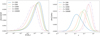 |
Fig. 1. Left: mass distribution of the Faraday rotation effect for various ℓ modes. Right: redshift distribution of the Faraday rotation effect for various ℓ modes. |
Figure 2 shows the angular power spectrum of the Faraday rotation angle for different values of the parameters β and μ of the spatial distribution profiles of the free electrons density and magnetic field, respectively. First, we note a shift of power to higher multipoles when increasing β or μ. Indeed the profile of free electrons and magnetic fields then becomes steeper so that they are more concentrated in the centre of the halo, which consequently appears smaller on the sky. This result is consistent with Tashiro et al. (2008). We also see that the difference in amplitudes is more significant when we change β rather than μ because β appears both in the free electrons and magnetic field profiles. However, the trend is different when changing β or μ. Indeed, when increasing μ, the amplitude decreases, as expected from the magnetic field profile Eq. (12). On the contrary, when increasing β, the amplitude also increases. This is because as the profile of free electrons is steeper, keeping the number of electrons constant; their concentration increases in Eq. (9), as does the amplitude.
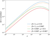 |
Fig. 2. Angular power spectra of the Faraday rotation angle, |

Figure 3 shows two different representations of the dependence of the angular power spectrum of the Faraday rotation angle on the amplitude of density fluctuation σ8: on the left we plot the angular power spectrum for different values of σ8 and on the right we plot the logarithmic derivative of the angular power spectrum with respect to σ8 as a function of ℓ. The latter gives the scaling of  with σ8, i.e. by writing
  then
then  .
.
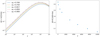 |
Fig. 3. Left: angular power spectra of the Faraday rotation angle, |


The angular power spectrum  is composed of the one-halo term only. Hence its scaling with σ8 is driven by the mass function, dN/dM, and the rotation angle at the core of haloes, αc. The latter does not explicitly depends on σ8. However, the scaling of dN/dM with σ8 is mass-dependent. Then the mass dependence of αc probes different mass ranges of the mass function, and as a consequence, different scaling of dN/dM with the amplitude of matter perturbations.
We find a dependence as  for ℓ = 10 and ℓ = 104, respectively. The power spectrum of the Faraday rotation angle is more sensitive to σ8 for low ℓ values than for high ℓ values because as seen above, the angular power spectrum is sensitive to higher mass at low ℓ and in this mass regime the mass function is more sensitive to σ8. We noticed that reducing the mass integration range from M = 1013 M⊙ to M = 5 × 10¹⁶ M⊙ (where it was [1010 M⊙, 5 × 10¹⁶ M⊙] before) slightly increases the power in σ8. This may be because the Faraday rotation effect is mainly sensitive to galaxy haloes with masses in the range M = 1013 to M = 1015 M⊙ (see Fig. 1) and that our mass function depends on σ8 more strongly from M = 1014 M⊙.
We note that the scaling in σ8 of the angular power spectrum is different than that for the tSZ angular power spectrum, which scales with  (see e.g. Hurier & Lacasa 2017). The reason is a different scaling in mass of the rotation angle at the core of haloes as compared to the tSZ flux; we note that the tSZ angular power spectrum is dominated by the one-halo contribution. Indeed, |αc|2 scales as M2, whereas the square of the tSZ flux at the core scales as M3.5. This results in a different weighting of the mass function, which is more sensitive to σ8 for high-mass values, the tSZ effect giving more weight to high masses than the Faraday rotation angle.
The dependence with σ8 found in this work is however different from that reported in Tashiro et al. (2008), the difference being mainly due to the presence of a two-halo term in Tashiro et al. (2008). The mass range [M = 1013 M⊙,5×1016 M⊙] is first considered in Tashiro et al. (2008) for which the angular power spectrum is dominated by its one-halo contribution9. In this case, the obtained scaling is  . The difference with the scaling found in this case lies in the reduced mass range, which gives more weight to the total effect to higher mass haloes. Second the mass range is extended in Tashiro et al. (2008) down to 1011 M⊙, leading then to a scaling as
  . In the mass range [1011 M⊙, 1013 M⊙], the two-halo term present in Tashiro et al. (2008) is not negligible anymore. This two-halo term then gives much more contribution to low-mass haloes as compared to ours (see Fig. 7 of Tashiro et al. 2008). However, the scaling of the two-halo term with σ8 is not driven anymore by
but instead by
where Pm(k, z) is the matter power spectrum (proportional to σ8). The steeper scaling with σ8 found in Tashiro et al. (2008) is thus mainly due to the non-negligible contribution of the two-halo term in their work.
We now want to study whether the Faraday rotation angle is sensitive to the matter density parameters. Keeping other cosmological parameters fixed, we have two possibilities to vary Ωm: either by varying the density of cold dark matter, ΩCDM, or that of baryons, Ωb.
We found that the Faraday rotation effect is almost independent of Ωm, when Ωb is kept fixed while varying ΩCDM, i.e.
for ℓ = 10 and ℓ = 104, respectively. This translates into a similar scaling with Ωm for a varying density of dark matter, i.e.
for ℓ = 10 and ℓ = 104, respectively.
However, when keeping ΩCDM fixed and varying Ωb, the dependence is clearly different and is written as
for ℓ = 10 and ℓ = 104, respectively. The resulting scaling with Ωm by varying the density of baryons is then
for ℓ = 10 and ℓ = 104, respectively. The dependence with Ωb and ΩCDM is simply understood by the fact the angular power spectrum scales with the fraction of baryons to the square. The effect is almost Ωm-independent when varying ΩCDM, as compared to the tSZ effect, which scales as  (Komatsu & Kitayama 1999). We can thus hope to use the Faraday rotation as a cosmological probe, by combining it with another physical effect having a different degeneracy in the Ωm − σ8 plane, such as the tSZ effect.
We finally study the effect of having a mass dependence of the (central) magnetic field strength owing to either an increase of this magnetic field strength with the mass of clusters, or by considering the higher values of magnetic fields for galaxies.
For the scaling with clusters mass first, we introduce B0(M)=Bp × (M/Mp)γ, where Mp = 5 × 10¹⁴ M⊙, Bp = 3 μG, and we let γ to vary from 0 to 1. The global amplitude of the power spectrum now scales with (Bp)2 while the mass scaling impacts the shape of the spectrum. We note that a change of Bp only changes the global amplitude of the power spectrum and not its scale dependence nor its response to changes in the cosmological parameters. The left panel of Fig. 4 shows  for five different values of γ. When increasing γ, the power spectrum is increased and the peak is shifted to lower ℓ values. Increasing the value of γ indeed leads to a higher contribution of massive haloes, which appears larger once projected on the sky, hence a peak at smaller multipoles. This shift to lower ℓ values and the difference in amplitude of the Faraday rotation angle could give insight into the scaling of the magnetic field strength with mass.
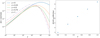 |
Fig. 4. Left: angular power spectra of the Faraday rotation angle, |


Figure 4 (right) shows how this mass dependence affects the dependence on σ8 of the Faraday rotation effect by plotting  with respect to γ. For ℓ = 100, when γ = 1, we find
  and we recover
  for γ = 0. In between,
  for γ = 0.25, 0.5, 0.75,-pagination
respectively. We stated a few lines above that our different scaling with σ8 of the angular power spectrum as compared to the thermal SZ effect came from a different scaling in mass. Indeed, the angular power spectrum of our effect scales as M2, where it scales as M3.5 for the tSZ effect, hence we recover the same scaling in σ8 for γ = 0.75. From this we also see that if we could model the magnetic field with a power-law mass dependence, the more it would depend on mass, the more the effect would be sensitive to σ8, allowing for a better determination of this cosmological parameter. Hence there is a correlation between the uncertainty on σ8 and the mass dependence of the magnetic field strength. The Faraday rotation angle still almost does not depend on Ωm (when varying ΩCDM only). Indeed,  for γ = 0, 0.25, 0.5, 0.75, and 1, respectively.
Second, the impact of a higher magnetic field in galaxies is taken into account using the hyperbolic tangent introduced in Eq. (15). We first only account for the increase in B for galaxies, i.e. no power-law scaling for clusters. This is shown as the dashed blue curve in Fig. 5, to be compared to the solid red curve where there is no mass scaling. It first increases the total power as a result of a globally higher magnetic field. The main impact is in the smallest scales since galaxies (which are low masses, hence smaller sized objects) now have an increased contribution because of the higher value of B0(M < 1013 M⊙). In this case, the scaling of  with σ8 is shifted to lower values as follows:
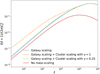 |
Fig. 5. Angular power spectrum for four models of the scaling of the magnetic field with the halo masses: (i) B0 = const. in solid red; (ii) an increase of the magnetic field for galaxies, i.e. at masses lower than 1013 M⊙ as given by Eq. (15) (dashed blue); and a combination of increased magnetic field for galaxies, Eq. (15), with a power law for massive clusters, Eq. (14), where (iii) γ = 0.25 (dotted green), and (iv) γ = 1 (dash-dotted orange). |
for ℓ = 10 and ℓ = 104, respectively. This change is because more weights are now attributed to lower haloes, hence probing a region of the mass function less sensitive to σ810.
We finally consider the two types of mass scaling simultaneously, i.e. an increase in the galaxy-mass range using tanh modelling, and an increase for massive cluster using a power law at masses above 5 × 10¹⁴ M⊙. This is depicted in Fig. 5 considering two values for the power law, i.e. γ = 0.25 in dotted green, and γ = 1 in dash-dotted orange. The scaling of the angular power spectra with the parameter σ8 now is
for ℓ = 10 and ℓ = 104, respectively. The case γ = 1 is particularly instructive. At large scales, dominated by massive cluster, we recover the scaling with σ8 mainly driven by the high-mass region of the mass function. At small scales however, the scaling is dominated by low-mass objects, hence much less sensitive to σ8. This has to be contrasted with the case of a magnetic field independent of the mass, for which the scaling with σ8 ranges from  to
to  for ℓ = 10 and ℓ = 104.
4.2. Power spectra of the Faraday conversion rate
First, we found no significative difference between the two angular power spectra of the Faraday conversion rate,  and
and  . Hence, for simplicity we now show results for the
  power spectrum only.
In Fig. 6, we compare the angular power spectra of the Faraday conversion rate for two populations of free electrons, either thermal or relativistic. In the case of the relativistic electrons, the central density in the halo is taken to be constant, contrary to the cold case which follows Eq. (9). We took the value  cm−3 corresponding to Γmin = 100 and βE = 2.5 (Colafrancesco et al. 2003). We note that with this specific choice for the spectral index we gets
  (see Sect. 2.3 and Colafrancesco et al. 2003). Since the amplitude of the angular power spectrum of the Faraday conversion rate is
  , we obtain
  , which scales as
  or conversely in terms of the Doppler factor as ∝1/Γmin. For such values describing relativistic electrons, we find that
  is ∼2 orders of magnitude higher in the thermal electron case compared to the relativistic case. This means that the number density of relativistic electrons should be pushed towards the unrealistic values of ∼10−3 cm−3 for the relativistic contribution to equal those of thermal electrons. This would correspond to a minimal Lorentz factor of Γmin ∼ 1, which is far below the values of ∼100 derived from the lifetime of relativistic electrons in the intracluster medium (Rephaeli 1979; Sarazin 1999).
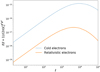 |
Fig. 6. Angular power spectra of the Faraday conversion rate |


The values of  used above are already over-optimistic with respect to the upper bound obtained on the number of cosmic rays (see Sect. 2.3). The contribution of relativistic electrons shown in Fig. 6 is thus a conservative upper bound, and we can safely neglect the case of relativistic electrons as compared to the contribution of thermal electrons.
4.2.1. Thermal electrons
The dependence of the angular power spectra of the Faraday conversion rate from thermal electrons on the density fluctuation amplitude σ8 is similar to that of the Faraday rotation angle: i.e.  for ℓ = 10 and ℓ = 104, respectively; the difference between low ℓ and high ℓ values has already been explained. The small differences with Faraday rotation come from the fact that the Faraday conversion rate for the angular power spectra scales as 1/(1 + z)6, where the conversion rate scales as 1/(1 + z)4 for the Faraday rotation angle.
As for the Faraday rotation effect, there is almost no variation of the Faraday conversion rate with Ωm, when varying ΩCDM and Ωb kept fixed, the dependence is written as

for ℓ = 10 and ℓ = 104, respectively.
When varying Ωm via Ωb instead (ΩCDM kept fixed), the dependence is not very different from Faraday rotation either, i.e.

for ℓ = 10 and ℓ = 104, respectively. Although these scalings are not very different from Faraday rotation, the same remark on the σ8 scaling differences applies here, which is that the two effects scale differently with redshift.
We also investigate the degeneracy between a scaling in mass of the magnetic field at the centre of the halo and the σ8 scaling, as what we have done for the Faraday rotation angle; see Fig. 7. The dependence in σ8 is  when γ = 1,
  when γ = 0.75,
  when γ = 0.5, and
  when γ = 0.25. When γ = 0.5 the angular power spectra scales with the mass to the four. This results in a scaling with σ8 to the power 9.5. For a comparison, it was also 9.5 for the Faraday rotation angle when it scaled with the mass to the four, corresponding for this case to γ = 1, so that our analysis is consistent.
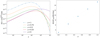 |
Fig. 7. Left: angular power spectra of the Faraday conversion rate, |


4.2.2. Relativistic electrons
We mention the case of Faraday conversion with relativistic electrons because the dependence of the angular power spectra with cosmological parameters is a bit different.
Indeed, when varying ΩCDM and Ωb kept fixed, the dependence is written as

for ℓ = 10 and ℓ = 104, respectively.
When varying Ωb and ΩCDM kept fixed, the dependence is written as

for ℓ = 10 and ℓ = 104, respectively.
This difference in dependence compared to the thermal electron case is explained by the constant value for the density of relativistic free electrons at the centre of the halo, whereas the density of cold free electrons at the centre scales with the fraction of baryons fb as well as the critical density ρc and the spherical overdensity Δ of the virialized haloes.
5. Conclusions
We revisited the derivation of the angular power spectrum of the Faraday rotation angle using the halo model and extended it to the case of Faraday conversion with an emphasis on the assumptions made for the statistics and orientations of magnetic fields inside haloes. Indeed, we first assumed the magnetic field of a halo to have a spherically symmetric profile but the same orientation over the halo scale. Second, the orientations are supposed to be uniformly distributed in the Universe to be consistent with the cosmological principle. Third, the orientations of magnetic fields in different haloes are independent from each other; the underlying idea is that magnetism is produced within halo in a local physical process. We also made the hypothesis that the distribution of the orientations of the magnetic fields inside haloes are independent from the abundance in mass and the spatial distribution of haloes. All of these hypotheses simplified the derivation of the angular power spectra: in particular, only the one-halo term remains because of the independence of the orientations from one halo to another.
We then explored the dependence of the angular power spectra with astrophysical and cosmological parameters. In Table 2, we report the scaling of the angular power spectra of the Faraday rotation angle and the Faraday conversion rate with the parameters σ8 and Ωm, assuming in this case that Ωm would vary by a change of the cold dark matter density. We also reported in this table the scaling for three other probes of the large-scale structures, namely halo number counts as observed through the tSZ effect, the tSZ angular power spectrum, and the angular power spectrum of CMB lensing potential.
Scaling of different large-scale-structure probes with σ8 and Ωm.
In particular, the angular power spectra of both Faraday rotation and Faraday conversion scale with the amplitude of the density fluctuations as  while it scales with
  to
to  for the other probes. However, this scaling with σ8 is degenerated with a mass-dependent magnetic field11. Still the scaling with the matter density parameter Ωm is in contrast to the tSZ and lensing probes: while for the SZ there is a scaling with
  , in this case it is almost independent of this parameter. Thus the two effects could be combined to lift the degeneracy in the σ8 − Ωm, assuming nonetheless the magnetic field mass-dependence model to be known. Conversely, a joint analysis could be used so as to infer the scaling of the magnetic fields with the masses of haloes.
Although other physical effects happen in the magnetized plasmas in haloes of galaxies, the dominant contributions are from Faraday rotation and Faraday conversion with thermal electrons as stated in Sect. 2. Indeed, an estimation of the angular power spectra of secondary anisotropies suggests that at 1 GHz, where a magnetic field of 10 μG and a density of relativistic electrons of nrel = 10−5 cm−3 for the absorption coefficients; there are 18 orders of magnitude between the secondary linearly polarized anisotropies produced thanks to Faraday rotation and those produced by absorption of intensity. Similarly, there are 9 orders of magnitude between the secondary circularly polarized anisotropies produced thanks to Faraday conversion and those produced by absorption of intensity. These differences in orders of magnitude do not change significantly when changing the frequency to 30 GHz and the magnetic field to 3 μG. Moreover, this is an ultra-conservative upper bound on such spectra since we consider in this paper a largely overestimated values for the number density of relativistic electrons. Thus, we can safely conclude that the secondary anisotropies induced by absorption would be negligible compared to the Faraday rotation and Faraday conversion induced anisotropies.
We note that this could also be done for the impact of the absorption coefficients since  .
.
This population is dubbed “cold plasma” in Sazonov (1969).
We note that in this case Faraday conversion and Faraday rotation by relativistic electrons are of equal magnitude. Faraday rotation by this population remains however much smaller than that due to thermal electrons.
We note that for two distinct haloes having however the same mass and are at the same redshift, it may well be that they share the same amplitude for B. This remains consistent with a statistically homogeneous and isotropic Universe as long as the orientations of the magnetic fields average down to zero.
We mention that the two-halo term may not be vanishing assuming some correlations between the magnetic fields of two different haloes; for example if these magnetic fields are seeded by a primordial magnetic field. In this case however, the two-halo term should be composed of a convolution of the matter power spectrum with the magnetic field power spectrum, as we could expect from results obtained for the similar case of the kinetic Sunyaev–Zel’dovich effect induced by the peculiar velocity of haloes (Hernandez-Monteagudo et al. 2006).
We note that abundances are given by a Poisson staistics for which  .
.
We note that in the above
![Mathematical equation: $$ \begin{aligned} \left\langle n_h(\boldsymbol{x}_i)n_h(\boldsymbol{x}_j)\right\rangle =\left(\frac{{\mathrm{d} } N}{{\mathrm{d} } M_i}\right)\left(\frac{{\mathrm{d} } N}{{\mathrm{d} } M_j}\right)\left[1+b(M_i,z_i)b(M_j,z_j)\xi _\mathrm{m} \left(\boldsymbol{x}_i-\boldsymbol{x}_j\right)\right], \end{aligned} $$](/articles/aa/full_html/2019/10/aa34485-18/aa34485-18-eq211.gif)
with b(M, z) the bias and ξm the two-point correlation function of the matter density field.
This is obviously a very simple approach. It is also possible to replace the profile U(x) by U(x)×s(x) so as to account for a more complex shape of the correlation function of the stochastic magnetic field; see for example Tashiro et al. (2008, 2009).
The angular power spectra derived in Tashiro et al. (2008) has a non-zero two-halo contribution.
This is, once again, to be compared with the scaling obtained in Tashiro et al. (2008). Accounting for galaxies with a central magnetic field of 10 μG, the scaling obtained in Tashiro et al. (2008) is  . The authors of Tashiro et al. (2008) however have a non-negligible contribution of the two-halo term which is vanishing in our study, hence the different scaling.
The impact of the scaling of B with the mass can be viewed as the equivalent of the mass bias in the analysis of the tSZ number counts and angular power spectrum.
This computation requires only three one-dimensional Fourier transforms.
Acknowledgments
The authors would like to thank G. Fabbian, S. Ilic, M. Douspis, and the entire COSM!X team for helpful discussions. J.G. acknowledges funding by the ByoPiC project from the European Research Council (ERC) under the European Union’s Horizon 2020 research and innovation programme grant agreement ERC-2015-AdG 695561. Part of the research described in this paper was carried out at the Jet Propulsion Laboratory, California Institute of Technology, under a contract with the National Aeronautics and Space Administration (NASA).
References
- Ade, P. A. R., POLARBEAR Collaboration, et al. 2014, Phys. Rev. Lett., 113, 021301 [NASA ADS] [CrossRef] [Google Scholar]
- Athreya, R. M., Kapahi, V. K., McCarthy, P. J., & van Breugel, W. 1998, A&A, 329, 809 [NASA ADS] [Google Scholar]
- Blasi, P., & Colafrancesco, S. 1999, Astropart. Phys., 12, 169 [NASA ADS] [CrossRef] [Google Scholar]
- Bonafede, A., Feretti, L., Giovannini, G., et al. 2009, A&A, 503, 707 [NASA ADS] [CrossRef] [EDP Sciences] [Google Scholar]
- Bonafede, A., Feretti, L., Murgia, M., et al. 2010, A&A, 513, A30 [NASA ADS] [CrossRef] [EDP Sciences] [Google Scholar]
- Campanelli, L., Dolgov, A. D., Giannotti, M., & Villante, F. L. 2004, ApJ, 616, 1 [NASA ADS] [CrossRef] [Google Scholar]
- Carroll, S. M. 1998, Phys. Rev. Lett., 81, 3067 [NASA ADS] [CrossRef] [Google Scholar]
- Carron, J., Lewis, A., & Challinor, A. 2017, JCAP, 1705, 035 [Google Scholar]
- Cavaliere, A., & Fusco-Femiano, R. 1978, A&A, 70, 677 [NASA ADS] [Google Scholar]
- Cavaliere, A., & Lapi, A. 2013, Phys. Rep., 533, 69 [NASA ADS] [CrossRef] [Google Scholar]
- Colafrancesco, S., Marchegiani, P., & Palladino, E. 2003, A&A, 397, 27 [NASA ADS] [CrossRef] [EDP Sciences] [Google Scholar]
- Cole, S., & Kaiser, N. 1988, MNRAS, 233, 637 [NASA ADS] [Google Scholar]
- Cooray, A., & Sheth, R. K. 2002, Phys. Rept., 372, 1 [Google Scholar]
- Cooray, A., Melchiorri, A., & Silk, J. 2003, Phys. Lett. B, 554, 1 [NASA ADS] [CrossRef] [Google Scholar]
- De, S., & Tashiro, H. 2015, Phys. Rev. D, 92, 123506 [NASA ADS] [CrossRef] [Google Scholar]
- Despali, G., Giocoli, C., Angulo, R. E., et al. 2016, MNRAS, 456, 2486 [NASA ADS] [CrossRef] [Google Scholar]
- Ejlli, D. 2017, Phys. Rev. D, 96, 023540 [NASA ADS] [CrossRef] [Google Scholar]
- Ejlli, D. 2018, Nucl. Phys. B, 935, 83 [NASA ADS] [CrossRef] [Google Scholar]
- Ejlli, D. 2019, Eur. Phys. J. C, 79, 231 [NASA ADS] [CrossRef] [EDP Sciences] [Google Scholar]
- Giodini, S., Lovisari, L., Pointecouteau, E., et al. 2013, Space Sci. Rev., 177, 247 [NASA ADS] [CrossRef] [Google Scholar]
- Giovannini, M. 2010, Phys. Rev. D, 81, 023003 [NASA ADS] [CrossRef] [Google Scholar]
- Govoni, F., Murgia, M., Feretti, L., et al. 2006, A&A, 460, 425 [NASA ADS] [CrossRef] [EDP Sciences] [Google Scholar]
- Hernandez-Monteagudo, C., Verde, L., Jimenez, R., & Spergel, D. N. 2006, ApJ, 643, 598 [NASA ADS] [CrossRef] [Google Scholar]
- Heyvaerts, J., Pichon, C., Prunet, S., & Thiébaut, J. 2013, MNRAS, 430, 3320 [NASA ADS] [CrossRef] [Google Scholar]
- Hirata, C. M., & Seljak, U. 2003, Phys. Rev. D, 68, 083002 [NASA ADS] [CrossRef] [Google Scholar]
- Huang, L., Liu, S., Shen, Z.-Q., et al. 2009, ApJ, 703, 557 [NASA ADS] [CrossRef] [Google Scholar]
- Huber, B., Tchernin, C., Eckert, D., et al. 2013, A&A, 560, A64 [NASA ADS] [CrossRef] [EDP Sciences] [Google Scholar]
- Hummel, E., Beck, R., & Dahlem, M. 1991, A&A, 248, 23 [NASA ADS] [Google Scholar]
- Hurier, G., & Lacasa, F. 2017, A&A, 604, A71 [NASA ADS] [CrossRef] [EDP Sciences] [Google Scholar]
- Kamionkowski, M. 2018, Phys. Rev. D, 97, 123529 [NASA ADS] [CrossRef] [Google Scholar]
- Kamionkowski, M., Kosowsky, A., & Stebbins, A. 1997, Phys. Rev. D, 55, 7368 [NASA ADS] [CrossRef] [Google Scholar]
- Kennett, M., & Melrose, D. 1998, PASA, 15, 211 [NASA ADS] [CrossRef] [Google Scholar]
- Kim, K. T., Kronberg, P. P., Giovannini, G., & Venturi, T. 1989, Nature, 341, 720 [NASA ADS] [CrossRef] [Google Scholar]
- Komatsu, E., & Kitayama, T. 1999, ApJ, 526, L1 [NASA ADS] [CrossRef] [PubMed] [Google Scholar]
- Kosowsky, A., & Loeb, A. 1996, ApJ, 469, 1 [NASA ADS] [CrossRef] [Google Scholar]
- Kosowsky, A., Kahniashvili, T., Lavrelashvili, G., & Ratra, B. 2005, Phys. Rev. D, 71, 043006 [NASA ADS] [CrossRef] [Google Scholar]
- Kunz, M. W., Schekochihin, A. A., Cowley, S. C., Binney, J. J., & Sanders, J. S. 2011, MNRAS, 410, 2446 [NASA ADS] [CrossRef] [Google Scholar]
- Li, M., & Zhang, X. 2008, Phys. Rev. D, 78, 103516 [NASA ADS] [CrossRef] [Google Scholar]
- LoVerde, M., & Afshordi, N. 2008, Phys. Rev. D, 78, 123506 [NASA ADS] [CrossRef] [Google Scholar]
- Lue, A., Wang, L.-M., & Kamionkowski, M. 1999, Phys. Rev. Lett., 83, 1506 [NASA ADS] [CrossRef] [Google Scholar]
- Mainini, R., Minelli, D., Gervasi, M., et al. 2013, JCAP, 1308, 033 [NASA ADS] [CrossRef] [Google Scholar]
- Makino, N., & Suto, Y. 1993, ApJ, 405, 1 [NASA ADS] [CrossRef] [Google Scholar]
- Marian, L., & Bernstein, G. M. 2007, Phys. Rev. D, 76, 123009 [NASA ADS] [CrossRef] [Google Scholar]
- Melrose, D. B., & McPhedran, R. C. 2005, Electromagnetic Processes in Dispersive Media, 431 (Cambridge: Cambridge University Press), [Google Scholar]
- Montero-Camacho, P., & Hirata, C. M. 2018, JCAP, 1808, 040 [NASA ADS] [CrossRef] [Google Scholar]
- Murgia, M., Govoni, F., Feretti, L., et al. 2004, A&A, 424, 429 [NASA ADS] [CrossRef] [EDP Sciences] [Google Scholar]
- Nagy, J. M., Ade, P. A. R., Amiri, M., et al. 2017, ApJ, 844, 151 [NASA ADS] [CrossRef] [Google Scholar]
- Ohno, H., Takada, M., Dolag, K., Bartelmann, M., & Sugiyama, N. 2003, ApJ, 584, 599 [NASA ADS] [CrossRef] [Google Scholar]
- Okamoto, T., & Hu, W. 2003, Phys. Rev. D, 67, 083002 [NASA ADS] [CrossRef] [Google Scholar]
- Planck Collaboration Int. XLVI. 2016, A&A, 596, A107 [NASA ADS] [CrossRef] [EDP Sciences] [Google Scholar]
- Pospelov, M., Ritz, A., Skordis, C., Ritz, A., & Skordis, C. 2009, Phys. Rev. Lett., 103, 051302 [NASA ADS] [CrossRef] [Google Scholar]
- Rephaeli, Y. 1979, ApJ, 227, 364 [NASA ADS] [CrossRef] [Google Scholar]
- Sarazin, C. L. 1999, ApJ, 520, 529 [NASA ADS] [CrossRef] [Google Scholar]
- Sawyer, R. F. 2015, Phys. Rev. D, 91, 021301 [NASA ADS] [CrossRef] [Google Scholar]
- Sazonov, V. N. 1969, Sov. Ast., 13, 396 [NASA ADS] [Google Scholar]
- Scoccola, C., Harari, D., & Mollerach, S. 2004, Phys. Rev. D, 70, 063003 [NASA ADS] [CrossRef] [Google Scholar]
- Seljak, U., & Hirata, C. M. 2004, Phys. Rev. D, 69, 043005 [NASA ADS] [CrossRef] [Google Scholar]
- Shcherbakov, R. V. 2008, ApJ, 688, 695 [NASA ADS] [CrossRef] [Google Scholar]
- Sherwin, B. D., & Schmittfull, M. 2015, Phys. Rev. D, 92, 043005 [NASA ADS] [CrossRef] [Google Scholar]
- Sigurdson, K., & Cooray, A. 2005, Phys. Rev. Lett., 95, 211303 [NASA ADS] [CrossRef] [Google Scholar]
- Simons Observatory Collaboration (Ade, P., et al.) 2019, JCAP, 1902, 056 [NASA ADS] [Google Scholar]
- Smith, K. M., Hanson, D., LoVerde, M., Hirata, C. M., & Zahn, O. 2012, JCAP, 1206, 014 [Google Scholar]
- Suzuki, A., Ade, P. A. R., Akiba, Y., et al. 2018, J. Low Temp. Phys., 193, 1048 [NASA ADS] [CrossRef] [Google Scholar]
- Takada, M., Ohno, H., & Sugiyama, N. 2001, [arXiv:astro-ph/0112412] [Google Scholar]
- Tashiro, H., Aghanim, N., & Langer, M. 2008, MNRAS, 384, 733 [NASA ADS] [CrossRef] [Google Scholar]
- Tashiro, H., Silk, J., Langer, M., & Sugiyama, N. 2009, MNRAS, 392, 1421 [NASA ADS] [CrossRef] [Google Scholar]
- Tinker, J., Kravtsov, A. V., Klypin, A., et al. 2008, ApJ, 688, 709 [NASA ADS] [CrossRef] [Google Scholar]
- Vacca, V., Murgia, M., Govoni, F., et al. 2012, A&A, 540, A38 [NASA ADS] [CrossRef] [EDP Sciences] [Google Scholar]
- Varshalovich, D., Moskalev, A., & Khersonskiĭ, V. 1988, Quantum Theory of Angular Momentum: Irreducible Tensors, Spherical Harmonics, Vector Coupling Coefficients, 3nj Symbols (World Scientific Pub.) [Google Scholar]
- Widrow, L. M. 2002, Rev. Mod. Phys., 74, 775 [NASA ADS] [CrossRef] [Google Scholar]
- Yadav, A. P. S., & Biswas, R., Su, M., & Zaldarriaga, M., 2009, Phys. Rev. D, 79, 123009 [NASA ADS] [CrossRef] [Google Scholar]
- Zaldarriaga, M., & Seljak, U. 1997, Phys. Rev. D, 55, 1830 [Google Scholar]
- Zaldarriaga, M., & Seljak, U. 1998, Phys. Rev. D, 58, 023003 [NASA ADS] [CrossRef] [Google Scholar]
Appendix A: Formal derivation of the angular power spectra for any effect considered
A.1. Radiative transfer coefficients
Looking at the expressions of the different radiative transfer coefficients reveals that they can assume two possible forms. These forms are first of scalar type as the Faraday rotation angle, and they read as an integral over the line of sight and over the halo distribution as follows:
![Mathematical equation: $$ \begin{aligned} \alpha (\boldsymbol{n})&=\displaystyle \int _0^{r_{\mathrm{CMB} }} a(r){\mathrm{d} } r \int \int {\mathrm{d} } M_i {\mathrm{d} }^3\boldsymbol{x}_i~n_h(\boldsymbol{x}_i)\nonumber \\ &\quad \times \left[\boldsymbol{b}(\boldsymbol{x}_i)\cdot \boldsymbol{n}\right]A\left(M_i, \left|\boldsymbol{x}-\boldsymbol{x}_i\right|\right). \end{aligned} $$](/articles/aa/full_html/2019/10/aa34485-18/aa34485-18-eq213.gif) (A.1)
(A.1)
In the above, the dependence over orientations is encoded in [b(xi)⋅n], which is a scalar function. The function A is the profile of the effect, which is for Faraday rotation by thermal electrons
 (A.2)
(A.2)
Since projection effects can only reduce the impact of the effect, the quantity A can be interpreted as the maximum of the effect a given halo can generate. Finally, nh is the halo distribution. The above scalar-type of coefficients are the Faraday rotation angle and the conversion from intensity to circular polarization, ϕI → V.
The second type of coefficients are those which are proportional to  , where B⊥ is the amplitude of the projected magnetic field on the plane orthogonal to the line of sight, and γ the angle between the projected magnetic field with the basis vector eθ in that plane. This is typical of the coefficients for Faraday conversion, ϕP → V, or conversion from intensity to linear polarization, ϕI → P. In terms of the amplitude of the magnetic field, B, and its orientation b, the phase is
 ![Mathematical equation: $ B^{2}_{\perp} e^{\pm2i\gamma}=B~\left[\boldsymbol{b}\cdot\left(\boldsymbol{e}_\theta\pm\mathrm{i}\boldsymbol{e}_\varphi\right)\right]^2 $](/articles/aa/full_html/2019/10/aa34485-18/aa34485-18-eq216.gif) . We thus have spin-( ± 2) coefficients reading as an integral over the line of sight as follows:
. We thus have spin-( ± 2) coefficients reading as an integral over the line of sight as follows:
![Mathematical equation: $$ \begin{aligned} i\phi ^{P\rightarrow V}(\boldsymbol{n})e^{\pm 2\mathrm{i}\gamma (\boldsymbol{n})}=&\displaystyle \int _0^{r_{\mathrm{CMB} }} a(r){\mathrm{d} } r \int \int {\mathrm{d} } M_i {\mathrm{d} }^3\boldsymbol{x}_i~n_h(\boldsymbol{x}_i)\nonumber \\&\times \left[\boldsymbol{b}\cdot \left(\boldsymbol{e}_\theta \pm \mathrm{i}\boldsymbol{e}_\varphi \right)\right]^2P\left(M_i,\left|\boldsymbol{x}-\boldsymbol{x}_i\right|\right). \end{aligned} $$](/articles/aa/full_html/2019/10/aa34485-18/aa34485-18-eq217.gif) (A.3)
(A.3)
The spin structure of the above is entirely encoded in projection coefficients [b⋅(eθ±ieφ)]2. The other terms are identical to those in scalar coefficients, except that the profile of the effect, P(r,|x−xi|), admits a different explicit expression, for example for Faraday conversion by thermal electrons
 (A.4)
(A.4)
Apart from the explicit expression of P, the formal expression of the coefficient remains the same for relativistic electrons or for conversion from intensity to linear polarization.
A formal expression for all the above radiative transfer coefficients can be abstracted from that above. On denoting ϕs any such coefficients, where s = 0 for scalar coefficients and s = ±2 for the spin coefficients, this is given by
 (A.5)
(A.5)
where Φ(r,|x−xi|) the profile amounting the maximum amount of the effect, which is a scalar function, and fs(bi, n) the function encoding the impact of projecting the magnetic field; the subscript i reminds us that the orientation is a priori a function of the haloes positions, xi. This is this last function which contains the spin structure of the considered coefficients.
A.2. Angular power spectrum
To compute the angular power spectrum, the usual approach consists in first computing the multipolar coefficients of ϕs(n) thanks to ϕs, ℓ, m = ∫dnϕs(n)s (n), and then to consider the two-point correlation between these multipolar coefficients,
  (superscripts 1, 2 labels two possibly different radiative transfer coefficients). The fields ϕs being statistically homogeneous and isotropic, the two-point correlation of multipolar coefficients is entirely described by an angular power spectrum, i.e.
  .
.
We adopt a slightly different path (totally equivalent though) by first considering the two-point correlation function on the sphere, denoted  , which is further simplified thanks to our assumption about the statistics of the magnetic fields orientations. The two-point correlation of the multipolar coefficients is secondly derived from the two-point correlation function via
  .
.
Assuming that orientations of the magnetic fields is not correlated to the spatial distribution of haloes leads to
![Mathematical equation: $$ \begin{aligned} \xi _{1,2}(\boldsymbol{n}_1,\boldsymbol{n}_2) =&\displaystyle \int _0^{r_{\mathrm{CMB} }} \left[a(r_1){\mathrm{d} } r_1\right]\left[a(r_2){\mathrm{d} } r_2\right]\nonumber \\ &\times \int \int \left[{\mathrm{d} } M_i{\mathrm{d} }^3\boldsymbol{x}_i\right]\left[{\mathrm{d} } M_j{\mathrm{d} }^3\boldsymbol{x}_j\right]\Phi ^{(1)}\nonumber \\&\times \left(M_i,\left|\boldsymbol{x}_1-\boldsymbol{x}_i\right|\right)\Phi ^{(2)}\left(M_j,\left|\boldsymbol{x}_2-\boldsymbol{x}_j\right|\right) \nonumber \\&\times \left\langle n_{\rm h}(\boldsymbol{x}_i)n_{\rm h}(\boldsymbol{x}_j)\right\rangle \left\langle f_s(\boldsymbol{b}_i,\boldsymbol{n}_1)f_{s{\prime }}(\boldsymbol{b}_j,\boldsymbol{n}_2)\right\rangle . \end{aligned} $$](/articles/aa/full_html/2019/10/aa34485-18/aa34485-18-eq225.gif) (A.6)
(A.6)
Since the orientation of the magnetic fields of two different haloes is uncorrelated, this gives ⟨fs(bi,n1)fs′(bj,n2)⟩ ∝ δi, j, and only the one-halo term contributes to the two-point cross-correlation function. In addition, these orientations are statistically homogeneous and isotropic, meaning that ⟨fs(bi,n1)fs′(bj,n2)⟩ is a function of |xi−xj| only. Because there is only the one-halo term, this relative distance is zero and ⟨fs(bi,n1)fs′(bj,n2)⟩ is a function of n1 and n2, i.e.  . Hence the two-point correlation function boils down to
![Mathematical equation: $$ \begin{aligned} \xi _{1,2}(\boldsymbol{n}_1,\boldsymbol{n}_2)=&\xi ^O_{s,s{\prime }}(\boldsymbol{n}_1,\boldsymbol{n}_2)\,\times \,\displaystyle \int _0^{r_{\mathrm{CMB} }} \left[a(r_1){\mathrm{d} } r_1\right]\left[a(r_2){\mathrm{d} } r_2\right]\nonumber \\&\times \int \int {\mathrm{d} } M_i{\mathrm{d} }^3\boldsymbol{x}_i\frac{{\mathrm{d} } N}{{\mathrm{d} } M}\Phi ^{(1)}\left(M_i,\left|\boldsymbol{x}_1-\boldsymbol{x}_i\right|\right)\Phi ^{(2)}\nonumber \\&\times \left(M_i,\left|\boldsymbol{x}_2-\boldsymbol{x}_i\right|\right), \end{aligned} $$](/articles/aa/full_html/2019/10/aa34485-18/aa34485-18-eq227.gif) (A.7)
(A.7)
where the mass function arises from the one-halo average of the abundance  . The function
  is interpreted as the correlation function of orientations, while the remaining term is the one-halo contribution of the two-point correlation function of the amplitude of the radiative transfer coefficient. Let us denote this second correlation function
  .
.
The full correlation function is thus a product of two correlation functions, one for the orientation and one for the amplitude of the coefficient, i.e.
 (A.8)
(A.8)
The correlation function of the amplitude,  , is formally identical to the one-halo term of the correlation function of, for example the tSZ effect, which is well known to be described by an angular power spectrum, i.e.
 (A.9)
(A.9)
where  is the angular power spectrum. Similarly, the correlation function of orientations is described by an angular power spectrum,
  , since this is a statisically homogeneous and isotropic field, i.e.
 (A.10)
We note that in the above, spin-weighted spherical harmonics are used to take into account the non-zero spins of the projected orientations.
Plugging Eqs. (A.9) and (A.10) into Eq. (A.8), and then taking the spherical harmonic transforms of ξ1, 2, we show that  can be expressed as a function of Gaunt integrals, the latter being defined as
 (A.11)
Gaunt integrals can be casted as products of Wigner-3j symbols. By then using triangular conditions and symmetries of the Wigner symbols (Varshalovich et al. 1988), we find
 (A.12)
The last summation over M and M′ of two Wigner-3js is equal to (2ℓ+1)−1 δℓ, ℓ′ δm, m′. We thus finally obtain that the correlation matrix of the multipolar coefficients is diagonal (as expected for statistically homogeneous and isotropic process), i.e.
 (A.13)
where the angular power spectrum of the Faraday effect is given by
 (A.14)
Since the two-point correlation function is the product of two two-point correlation functions, we consistently find that the angular power spectrum is the convolution of the respective two angular power spectra  and
and  .
.
Appendix B: Derivation of 
B.1. Uniformly oriented magnetic field
We describe the derivation of the expression of  . This is very reminiscent to the calculation of the angular power spectrum of, for example the tSZ effect (see e.g. Cole & Kaiser 1988; Makino & Suto 1993; Komatsu & Kitayama 1999), simplified in this work since we only need to derive the one-halo term. To this end let us define
  such that
 (B.1)
(B.1)
Then  is the angular power spectrum of the above quantity restricted to its one-halo contribution.
The integral over xi in A(n) is the convolution of the halo abundance, nh, where the profile of the halo, X. This is then written as a product in Fourier space to get
 (B.2)
(B.2)
where  means the three-dimensional Fourier transform of f(xi). Because the radial profile is spherically symmetric, it only depends on the norm of the wavevector k ≡ |k| and can be expressed using spherical Bessel functions
 (B.3)
(B.3)
where R ≡ |x−xi| and j0 is the spherical Bessel function at order ℓ = 0. We further make use of the Rayleigh formula to express the eik ⋅ x using spherical Bessel functions and spherical harmonics. The multipolar coefficients are then obtained through  leading to
 (B.4)
(B.4)
The two-point correlation of the above set of multipolar coefficients involves the auto-correlation of the Fourier transform of the halo abundance. The Poisson part of the two-point correlation of the halo density field is  where dN/dMi is the mass function. The corresponding power spectrum is constant (independent of scale):
  . Thanks to the scale independence of this power spectrum and to the fact that the Fourier-transformed profile of the angle depends on k only, we can perform the integral over (k/k) to get
 (B.5)
(B.5)
where the angular power spectrum is written as
 (B.6)
(B.6)
The numerical evaluation of the angular power spectrum DL as derived above is still prohibitive because of the presence of the highly oscillating Bessel functions. It is however built from expressions of the form
which can be simplified using the Limber approximation (LoVerde & Afshordi 2008). Using this approximation, we obtain
 (B.7)
(B.7)
We finalize our expression of the angular power spectrum  by introducing the projected Fourier transform of the profile. To this end, we first note that X(R)=X(c)(M, z, Bc) U(R/Rc), where Bc is the mean magnetic field strength at the centre of the halo (which can also depend on M and z; see Tashiro et al. (2008)), and U is a normalized profile which only depends on the ratio of the comoving distance from the centre, R, to the typical comoving radius of the halo, Rc, which is also a function of z and M. For a β-profile, this is written as
  and U(R/Rc)=(1 + R/Rc)−3β(1 + μ)/2.
Introducing the variable x = R/Rc and physical radius of the halo,  , we find
where  , which is the typical multipole associated with the typical size of the halo (the latter being also a function of M and z through
  ), and Dang(z) the angular diameter distance. By defining the projected Fourier transform of the profiles
 (B.8)
(B.8)
the angular power spectrum DL is then written as
 (B.9)
(B.9)
B.2. Adding a stochastic contribution to the magnetic field
Adding a contribution of a stochastic component to the magnetic field is done by amending Eq. (B.4) as follows: we replace the Fourier transform of the profile X([x−xi|) by
 (B.10)
where  is a stochastic variable described by a statistically isotropic power spectrum. This is just the convolution of the profile with some random component described by a power spectrum. This gives for the two-point correlation of the multipolar coefficients
 (B.11)
We note that only the diagonal of the spectrum, i.e.  , is involved here, and not the off-diagonal terms, i.e.
  with k ≠ k′. This is because the statistical average of the halo abundance, i.e.
  , is proportional to δ3(k − k′). Although in this case we are only interested in the one-halo term, this would equally apply to the two-halo term with the addition, however, of the matter power spectrum.
It can be shown that the power spectrum of the random variable  is also isotropic, i.e. a function of k only, as follows: We first note
 (B.12)
where we use the fact that  is a statistically isotropic random field, i.e.
  . Hence
  is the convolution of the Fourier coefficients of two functions which are spherically symmetric, since both
  and
and  are functions of the wavenumber only. Hence we rewrite this in real-space (leading then to a product of two spherically symmetric functions) as follows:
 (B.13)
where the inverse-Fourier transform introduced above reads
 (B.14)
 (B.15)
We note that r can be understood as a mere dummy variable. We also stress that X2(r) should not be confused with |X(r)|2. Finally, the function S(r) is no more than the correlation function introduced in Sect. 2.3.
It is then clear that  can be replaced by
  where it is now a function of the wavenumber only. We can thus perform in Eq. (B.11) the integral over (k/k) to get δL, L′δM, M′. We thus obtain
  ;the amended angular power spectrum reads
 (B.16)
where the new power spectrum of haloes,  , is obtained from the Fourier transform of the β-profile,
  , and the power spectrum of the stochastic component,
  , using the set of Eqs. (B.13)–(B.15)12.
Let us now discuss how this impact  as compared to the simplifying assumption of uniform orientation of the magnetic field up to the virial radius. This basically consists in comparing
  to
to  . We first note to ease the comparison that the latter is directly derived from the former by setting S(r) = 1. Hence we need to compare
 (B.17)
to
 (B.18)
Assuming self-similarity, we can write S(r)=Sc(M)×s(r/rc), where Sc is some amplitude (potentially mass-dependent), and s(r/rc) a shape function depending on the ratio r/rc only, and which decreases to zero at scales smaller than the virial radius. At a qualitative level then, adding the stochastic contribution leads to two effects. First, the shape function introduces a universal smoothing hence suppressing power at large scales. The second impact comes from the peculiar scaling with the mass which might give more or less weights for haloes with different masses. This additional scaling however can be fully incorporated within the mass scaling of Bc.
The function X2(r) is no more than the convolution of the profile X(r) with itself. Hence we can introduce an effective profile, Xeff(r), accounting for the stochastic contribution as the function such its auto-convolution product equals X2(r)S(r), i.e. ∫dxXeff(r)Xeff(r − x)=X2(r)S(r). This effective profile should then account for the additional smoothing introduced by s(r) plus some potential additional scaling of the total amplitude of the effect with the mass; the latter is however easily absorbed into the scaling Bc(M). Armed with such an effective profile, all the analytical expressions derived in the previous section of this appendix can be directly used replacing X by Xeff.
Appendix C: Derivation of  for Faraday rotation
The angular power spectrum  for Faraday rotation is obtained through the computation of the correlation ⟨b(n1,xi)b(n2,xj)⟩. We note that b(n, xi)=n ⋅ b(xi). We use the vector basis (ez, e+, e−), where
  and (ex, ey, ez) is the standard Cartesian basis of ℝ3. The components of the orientation of the magnetic field b and the line-of-sight direction n are given by
 (C.1)
(C.1)
We note that in the specific reference frame adopted in this case, the components of the line-of-sight unit vector are expressed using the spherical harmonics for ℓ = 1. This way of expressing the components of the unit vector of the line of sight is appropriate for further reading the angular power spectrum from the two-point correlation function; see Eq. (A.10).
For uniformly distributed unit vectors, we obtain the following average:
 (C.2)
(C.2)
which is only non-zero for the same haloes. This is also constant in space because, as explained in Appendix A, it results from an homogeneous and isotropic process. The two-point correlation function finally is writen as
 (C.3)
(C.3)
from which the angular power spectrum is easily obtained to be  .
.
Appendix D: Derivation of  for Faraday conversion
In this appendix we compute the following two-point correlation functions: ⟨b±2(n1,xi)b±2(n2,xj)⟩ and ⟨b±2(n1,xi)b∓2(n2,xj)⟩ where we note that b±2(n,xi) ≡ [b(xi)⋅(eθ ± ieφ)]2. Working in the basis (ez, e+, e−) as used in Appendix B, squares of inner-dot products b±2(n,xi) are conveniently expressed as
 (D.1)
(D.1)
where the five coefficients bμ depend on the orientations of the magnetic fields only (i.e. they are functions of β(xi) and α(xi) only). They are given by
 (D.2)
(D.2)
The five coefficients  are functions of the line of sight only and with our choice of the reference frame, they are expressed using spin-weighted spherical harmonics for s = ± 2 and ℓ = 2, i.e.
 (D.3)
(D.3)
Ensemble averages are done for the bμ coefficients, which for a uniform distribution of orientations gives ⟨bμ(xi) bν(xj)⟩ = δμ, ν δi, j. The different correlation functions are then given by
 (D.4)
(D.4)
 (D.5)
(D.5)
All these correlation are thus described by the angular power spectrum (which is non-zero for the one-halo term only) written as  .
.
All Tables
Scaling of the radiative transfer coefficients for thermal electrons and relativistic electrons with the projection of the magnetic fields along or orthogonal to the line of sight, the frequency of photons, and the density and temperature of free electrons (adapted from Sazonov 1969).
All Figures
|
Fig. 1. Left: mass distribution of the Faraday rotation effect for various ℓ modes. Right: redshift distribution of the Faraday rotation effect for various ℓ modes. |
| In the text | |
|
Fig. 2. Angular power spectra of the Faraday rotation angle, |
| In the text | |
|
Fig. 3. Left: angular power spectra of the Faraday rotation angle, |
| In the text | |
|
Fig. 4. Left: angular power spectra of the Faraday rotation angle, |
| In the text | |
|
Fig. 5. Angular power spectrum for four models of the scaling of the magnetic field with the halo masses: (i) B0 = const. in solid red; (ii) an increase of the magnetic field for galaxies, i.e. at masses lower than 1013 M⊙ as given by Eq. (15) (dashed blue); and a combination of increased magnetic field for galaxies, Eq. (15), with a power law for massive clusters, Eq. (14), where (iii) γ = 0.25 (dotted green), and (iv) γ = 1 (dash-dotted orange). |
| In the text | |
|
Fig. 6. Angular power spectra of the Faraday conversion rate |
| In the text | |
|
Fig. 7. Left: angular power spectra of the Faraday conversion rate, |
| In the text | |
Current usage metrics show cumulative count of Article Views (full-text article views including HTML views, PDF and ePub downloads, according to the available data) and Abstracts Views on Vision4Press platform.
Data correspond to usage on the plateform after 2015. The current usage metrics is available 48-96 hours after online publication and is updated daily on week days.
Initial download of the metrics may take a while.