| Issue |
A&A
Volume 698, May 2025
|
|
|---|---|---|
| Article Number | A208 | |
| Number of page(s) | 18 | |
| Section | Extragalactic astronomy | |
| DOI | https://doi.org/10.1051/0004-6361/202452978 | |
| Published online | 17 June 2025 | |
A negative stellar mass−gaseous metallicity gradient relation of dwarf galaxies modulated by stellar feedback
1
Key Laboratory for Research in Galaxies and Cosmology, Department of Astronomy, University of Science and Technology of China, Hefei 230026, China
2
School of Astronomy and Space Science, University of Science and Technology of China, Hefei 230026, China
3
Department of Astronomy and Astrophysics, University of California Santa Cruz, 1156 High Street, Santa Cruz, CA 95064, USA
4
Sub-department of Astrophysics, University of Oxford, Keble Road, Oxford OX1 3RH, UK
5
Deep Space Exploration Laboratory/Department of Astronomy, University of Science and Technology of China, Hefei 230026, People’s Republic of China
6
Frontiers Science Center for Planetary Exploration and Emerging Technologies, University of Science and Technology of China, Hefei, Anhui 230026, People’s Republic of China
7
European Southern Observatory, Alonso de Cordova 3107, Casilla, 19001 Vitacura, Santiago 19, Chile
8
School of Astronomy and Space Science, Nanjing University, Nanjing 210093, China
9
Key Laboratory of Modern Astronomy and Astrophysics (Nanjing University), Ministry of Education, Nanjing 210093, China
10
Instituto de Estudios Astrofísicos, Facultad de Ingeniería y Ciencias, Universidad Diego Portales, Av. Ejército Libertador 441, Santiago, Chile
11
Department of Astronomy, Tsinghua University, Beijing, Beijing 100084, China
12
Department of Astronomy, Westlake University, Hangzhou, 310030 Zhejiang Province, China
13
Department of Astronomy and Institute of Theoretical Physics and Astrophysics, Xiamen University, Xiamen 361005, China
14
School of Astronomy and Space Science, University of Chinese Academy of Sciences (UCAS), Beijing 100049, People’s Republic of China
15
National Astronomical Observatories, Chinese Academy of Sciences, Beijing 100101, People’s Republic of China
16
Institute for Frontiers in Astronomy and Astrophysics, Beijing Normal University Beijing 102206, People’s Republic of China
17
College of Physics and Electronic Engineering, Qujing Normal University, Qujing, Yunnan 655011, China
⋆ Corresponding author: hzhang18@ustc.edu.cn
Received:
13
November
2024
Accepted:
22
April
2025
Baryonic cycling is reflected in the spatial distribution of metallicity within galaxies; however, gas-phase metallicity distribution and its connection with other properties of dwarf galaxies are largely unexplored. We present the first systematic study of radial gradients of gas-phase metallicities for a sample of 55 normal nearby star-forming dwarf galaxies (stellar mass M⋆ ranging from 107 to 109.5 M⊙) based on MUSE wide-field spectroscopic observations. We find that the metallicity gradient has a significant negative correlation (Spearman’s rank correlation coefficient r ≃ −0.56) with M⋆, which is in contrast with the flat or even positive correlation observed for higher-mass galaxies. The negative correlation is accompanied by a stronger central suppression of metallicity compared to the outskirts in lower-mass galaxies. Among the other explored galaxy properties, including baryonic mass, star formation distribution, galaxy environment, regularity of gaseous velocity field, and effective yield of metals yeff, only the regularity of gaseous velocity field and yeff have residual correlation with metallicity gradient after controlling for M⋆, in the sense that galaxies with an irregular velocity field or lower yeff favor a less negative or more positive metallicity gradient. Particularly, a linear combination of logarithmic stellar mass and yeff significantly improves the correlation with metallicity gradients (r ∼ −0.68) compared to using stellar mass alone. The lack of correlation with environment disproves gas accretion as a relevant factor shaping the metallicity distribution. The correlation with both gaseous velocity field regularity and yeff implies the importance of stellar feedback-driven metal redistribution within the ISM. Our finding suggests that the metal mixing and transport process, including but not limited to feedback-driven outflow, are more important than in situ metal production in shaping the metallicity distribution of dwarf galaxies.
Key words: galaxies: abundances / galaxies: dwarf / galaxies: evolution / galaxies: ISM / galaxies: star formation
© The Authors 2025
 Open Access article, published by EDP Sciences, under the terms of the Creative Commons Attribution License (https://creativecommons.org/licenses/by/4.0), which permits unrestricted use, distribution, and reproduction in any medium, provided the original work is properly cited.
This article is published in open access under the Subscribe to Open model. Subscribe to A&A to support open access publication.
1. Introduction
Metallicity of the interstellar medium (ISM) serves as a chemical clock of the evolutionary status of its host galaxy. In an idealized closed-box scenario, a galaxy’s metallicity is solely determined by the total fraction of gas converted into stars and the stellar yields. In reality, however, metallicity may be subject to modulation by gas accretion from outside or gas outflow driven by feedback processes inside the galaxy (Finlator & Davé 2008; Peng & Maiolino 2014). Therefore, ISM metallicity and its spatial distribution can be used to probe galaxy formation history and the accompanied baryon cycle.
Studies in the past have found several galaxy scaling relations involving gas metallicity, such as the well-known mass-metallicity (M−Z) relation (e.g., Lequeux et al. 1979; Tremonti et al. 2004; Yao et al. 2022) and the fundamental metallicity relation (FMR) (e.g., Mannucci et al. 2010; Li et al. 2023; Bulichi et al. 2023). These studies generally reveal a strong positive correlation between metallicity and galaxy mass and a negative correlation between metallicity and star formation rate (or gas content) for a given galaxy mass.
The recent advent and widespread use of integral field unit (IFU) spectroscopy, many large surveys, such as the Calar Alto Legacy Integral Field Area survey (CALIFA, Sánchez-Menguiano et al. 2016), the Mapping Nearby Galaxies at APO (MaNGA, Bundy et al. 2015), and the Sydney-AAO Multi-object Integral-field unit survey (SAMI, Bryant et al. 2015) make it possible to derive a relatively accurate 2D distribution of stellar populations, stellar or gaseous kinematics, and metallicities for large samples of galaxies.
The spatial distributions of gas-phase metallicity in galaxies are usually quantified by the gradient of its radial profiles. Negative gradients of the radial metallicity profiles have been found in most of relatively massive disk galaxies in the Local Universe (e.g., Zaritsky et al. 1994; Sánchez-Menguiano et al. 2016; Pilyugin et al. 2014). This negative gradient is in line with an inside-out formation scenario of the disks (Peng & Maiolino 2014), that is, the inner regions of galaxies were first and more efficiently formed by earlier accumulation of gas with low angular momentum (and thus more efficient chemical enrichment), while the gas with higher angular momentum settles in the outer disks at a lower pace and forms stars less efficiently. In addition, metal-enriched gas inflow along galaxy disks may also contribute to the negative metallicity gradient (e.g., Wang & Lilly 2022; Wang et al. 2024).
While the studies mentioned above have shown that local spiral galaxies generally have a negative gas-phase metallicity gradient, its dependence on various galaxy properties and environments is still not clear. Some recent studies found that gas-phase metallicity gradients are sensitive to galaxy morphology (e.g., Kreckel et al. 2019) and environment (e.g., Lara-López et al. 2022). A scaling relation between galaxy stellar mass and metallicity gradient was found by some recent work. Belfiore et al. (2017) measured the metallicity gradients of a sample of galaxies (log(M⋆/M⊙) > 9) from the MaNGA survey, and found that galaxies with intermediate stellar masses (log(M⋆/M⊙) ∼ 10.5) have the steepest metallicity gradients, and the gradients flatten toward both the lower-mass and higher-mass end. Similar results are also found in SAMI galaxies (Poetrodjojo et al. 2021). Recent simulations (e.g., Hemler et al. 2021) and theoretical works (e.g., Sharda et al. 2021a) have made significant progress in understanding the physical processes that shape the metallicity gradients.
Generally speaking, IFU spectroscopy is superior to traditional long-slit spectroscopy in probing the spatial distribution of metallicity in galaxies. However, the majority of existing large IFU surveys (e.g., Bundy et al. 2015; Sánchez-Menguiano et al. 2016; Bryant et al. 2015) are biased to relatively massive galaxies. Our current knowledge of metallicity distribution in nearly dwarf galaxies is largely from earlier long-slit spectroscopic observations of selected H II regions. A general conclusion from previous studies is that dwarf galaxies usually lack a significant metallicity gradient (e.g., Pagel et al. 1978; Roy et al. 1996; Hunter & Hoffman 1999; van Zee & Haynes 2006; Lee et al. 2007; Croxall et al. 2009). Nevertheless, Pilyugin et al. (2015) measured abundance distribution of 14 dwarf irregular galaxies, and found that the metallicity gradient appears to be steeper in galaxies with steeper surface brightness profiles. Due to the faintness and low surface brightness of ordinary star-forming dwarf galaxies, it is observationally expensive to obtain unbiased metallicity distributions for relatively large samples of dwarf galaxies, and only a few studies attempted to fully explore the mass- and morphology-dependence of metallicity gradients of galaxies by including a small sample of dwarf galaxies (e.g., Ho et al. 2015; Bresolin 2019). More work is needed to extend the relation between the metallicity gradient and other galaxy properties to the lower-mass end.
For this paper we collected a sample of nearby dwarf galaxies with available MUSE IFU spectroscopic observations; our aim is to extend the stellar mass−gaseous metallicity gradient relation (MZGR) studies to the dwarf galaxy regime, and attempt to explore the physical drivers of the metallicity distribution of dwarf galaxies. This paper is organized as follows. In Sect. 2, we describe the sample selection and data reduction. The data analysis is presented in Sect. 2.4. We present our result in Sect. 3 and the discussion in Sect. 4. The summary and our conclusion are given in Sect. 5. Throughout the paper we assume a cold dark matter ΛCDM cosmology with H0 = 70 km s−1 Mpc−1, Ωm = 0.3 and ΩΛ = 0.7.
2. Sample and data reduction
2.1. Description of MUSE
The Multi Unit Spectroscopic Explorer (MUSE; Bacon et al. 2010) is an integral-field spectrograph installed on UT 4 of the Very Large Telescopes (VLT) at the Cerro Paranal Observatory. In its wide-field mode, MUSE has a field of view (FOV) of 1′×1′ with a spatial sampling of 0.2″ × 0.2″ (i.e., 0.02 kpc at a distance of 20 Mpc), a spectral sampling of 1.25 Å, and a spectral resolution of 1770 at 465 nm to 3590 at 930 nm.
2.2. Sample selection
The parent sample of nearby galaxies (< 30 Mpc) with B-band absolute magnitude fainter than −18.5 mag was retrieved from the extragalactic database Hyperleda1. We then searched for wide-field mode MUSE observations of these galaxies in the ESO Science Archive2. To achieve a reasonable signal-to-noise ratio for emission line detection, we required an on-source exposure time of at least 2000 seconds. To have an adequate spatial coverage for gradient measurement, we further required the MUSE observations to cover at least out to one effective radius Re of a galaxy. It turns out that 72 galaxies satisfy the above criteria, and their MUSE data were retrieved. As will become clear in Sect. 2.4, 36 of the 72 galaxies are active star-forming galaxies with decent detection of nebular emission lines that can be used to measure the gas-phase metallicity distribution. These 36 galaxies will be used to explore the metallicity gradients in this work.
In addition, a subset of sources from the Dwarf Galaxy Integral-field Survey (DGIS)3 (Li et al. 2025) is also incorporated into our sample. DGIS aims to acquire observations with spatial resolutions as high as 10–100 pc while maintaining reasonably high signal-to-noise ratios with VLT/MUSE and ANU-2.3m/WiFeS. The whole sample is composed of 65 dwarf galaxies with M⋆ < 109 M⊙, selected from the Spitzer Local Volume Legacy Survey. We selected the subset of their sample that has MUSE observations (40 sources) and meets our galaxy selection criteria (19 of 40). This brings the total sample size to 55. We use the datacubes calibrated by the DGIS team, but the metallicity gradient and other relevant measurements used in this work were derived by us in a consistent manner with the other galaxies in our sample. The information of these 55 galaxies is given in Table A.1.
2.3. MUSE data reduction
We downloaded the raw science data and calibration files from the archive data center. The data reduction was performed using MUSE pipeline in the EsoReflex environment (Freudling et al. 2013). EsoReflex employs a workflow engine that provides a visual guidance of the data reduction cascade, including the standard processes such as wavelength and flux calibration, sky subtraction, cosmic-ray rejection, and combination. Particularly, for sky subtraction, we used dedicated offset sky exposures if available; otherwise we carefully chose sky regions near the edge of the science observations.
Before combining the individual exposures calibrated through the pipeline, we performed a visual inspection of spectra extracted from the central regions of individual exposures, in order to find and exclude corrupted observations (due to either poor weather conditions or instrumental failures) from the final combination. Out of 72 galaxies, 6 were excluded from our sample for this reason, bringing the sample to 66. After combining the valid exposures, we used the Zurich Atmosphere Purge package (ZAP; Soto et al. 2016) to further improve sky subtraction. With the combined spectral cubes in hand, we used the utility muse_cube_filter in the MUSE pipeline to generate broadband images over the SDSS g, r, i, z filters by integrating the data cube in the wavelength direction. These broadband images will be used to improve the flux calibration (see below).
2.4. Refinement of the MUSE flux calibration
Flux calibration of the MUSE spectra may be subject to significant uncertainties in a relative and (especially) absolute sense. To remedy this potential problem, we turned to the broadband (g, r, i, z) images from the Dark Energy Spectroscopic Instrument (DESI) Legacy Imaging Surveys4. Because the MUSE field does not always contain isolated bright point sources that are ideal for flux calibration, we decided to perform the calibration by comparing integrated flux over the same central area of our galaxies on the DESI images and the above generated MUSE images. For galaxies with isolated point sources falling in the MUSE field, we also performed the flux calibration with the isolated point sources as a sanity check, and find that the two methods agree with each other within 1 percent.
We find that the ratios of broadband flux measured from the MUSE and DESI images of our galaxies fall in a narrow range of 0.9–1.1, without significant wavelength dependence. Therefore, we chose to apply the scaling factors derived from the r band calibration of each galaxy to the MUSE data cubes to avoid the influence of residual sky lines and incomplete wavelength coverage of MUSE over the broadband (i.e., g, z). Four galaxies (ESO489-G56, NGC 2915, UGCA116, UGC3755) in our sample do not have DESI images, so we did not attempt to refine their absolute flux calibration.
2.5. Photometric and geometric parameters
To prepare for exploring the radial distribution of metallicity and other properties of our sample galaxies, we need to obtain the relevant geometric parameters with broadband images. To do this, we used the elliptical isophote analysis tools in the Python package PHOTUTILS (Bradley et al. 2024). In particular, we determined the galactic center, ellipticity, and major-axis position angle (PA) directly based on isophote fitting to the above generated MUSE r-band images, and then used the same ellipse geometry parameters to determine the major-axis effective radius Re based on the DESI r-band images. We note that the MUSE r-band images are used to measure all the above-mentioned parameters for the four galaxies without DESI images. One galaxy (NGC 1487) was excluded from the sample in this step because it involves a close interaction between three galaxies. The measurements are given in Table A.1. We have compared our measurements of the geometry parameters with those reported in the HyperLeda database, and confirm that they are generally consistent with each other within uncertainties (e.g., Δ(PA) = − 1.7 ± 34.3, Δ(e) = − 0.016 ± 0.13).
2.6. Spectral fitting and emission-line measurement
A robust emission line measurement requires a careful stellar continuum modeling. We follow a workflow similar to the MaNGA Data Analysis pipeline (DAP, Westfall et al. 2019) to analyze our MUSE data cubes. The workflow involves three major parts: a hybrid binning scheme for continuum and emission lines, spectral fitting of the continuum with stellar population models, and emission line measurement on continuum-subtracted spectra.
Before performing the analysis, we masked out the spaxels contaminated by foreground stars or background galaxies, and corrected the data cubes for the Galactic extinction by adopting the Schlegel et al. (1998) extinction map and the Cardelli et al. (1989) extinction law. To perform the continuum modeling, we first used the Voronoi tessellation method (VorBin, Cappellari & Copin 2003) to adaptively rebin the spaxels to achieve a minimum continuum S/N of 50 Å−1 (near 5500 Å), and then fitted the stacked spectra of each rebinned spaxel with the Penalized Pixel cross-correlation Fitting (pPXF, Cappellari 2017) package. Residual sky lines and nebular emission lines were masked during the continuum fitting, and the fitting is restricted to a wavelength range from 4800 to 7200 Å to avoid contamination from residual sky lines at redder wavelengths and the boundaries of MUSE spectra. We used the E-MILES stellar population models (Vazdekis et al. 2016) and followed the same strategy as Tang et al. (2022) to perform pPXF fitting. The reader is referred to Tang et al. (2022) for more details.
After obtaining the best-fit continuum model for each Voronoi bin, we rescaled the continuum model to match that of the observed spectrum of each individual spaxel in the same Voronoi bin, and then subtracted the scaled model spectra from individual spaxels. We then estimated S/N and equivalent width (EW) of nebular emission lines, including Hα, Hβ, [O III]λ5007, [N II]λ6583, [S II]λ6716, and [S II]λ6731, based on the continuum-subtracted spectra of individual spaxels. Out of 93 galaxies, 28 have no emission line detection and were thus excluded from the following analysis. Next, we performed Voronoi binning of the original spaxels to achieve a minimum S/N ∼ 10 in the weakest emission lines mentioned above. Spaxels with Hα equivalent width < 5 Å may have a significant contribution from the so-called Diffuse Ionized Gas (DIG), for which the existing metallicity calibration methods may not be valid (e.g., Sanders et al. 2017; Zhang et al. 2017). So these low EW(Hα) spaxels were masked during the Voronoi binning above and excluded from the following analysis.
We performed Gaussian profile fitting to each emission line of the Voronoi-binned spaxels to determine the line flux, central velocity, and velocity dispersion. To correct for internal dust extinction of the emission lines, we adopted the Balmer decrement method by assuming an intrinsic Hα/Hβ = 2.86 for a Case B recombination with a temperature of 10 000 K and an electron density of 100 cm−3 (Hummer & Storey 1987). The Cardelli et al. (1989) dust-attenuation law is used for the extinction correction. We note that a zero dust extinction is assigned to spaxels with an observed Hα/Hβ < 2.86. Lastly, we used the log([OIII]λ5007/Hβ) vs. log([NII]λ6584/Hα) Baldwin-Phillips-Terlevich (BPT; Baldwin et al. 1981)) diagram to exclude spaxels that are inconsistent with being pure star-forming regions, based on the division line of Kauffmann et al. (2003) on the BPT diagram. We note that the WHaD method proposed by Sánchez et al. (2024) provides an overall consistent classification of star-forming spaxels with the WHα+BPT method adopted in this work, as already pointed out by Sánchez et al. (2024). After this step, 59 galaxies (out of 65) have at least 10 Voronoi-binned star-forming spaxels. In the end, we re-examined the metallicity distribution in our sample galaxies by visual inspection, and find 4 galaxies (ESO59-01, ESO320-14, ESO321-14, VCC0170) have only metallicity measurements that cover very small radial range or a single star-forming region. These 4 galaxies were excluded from the following analysis. The remaining 55 galaxies constitute the final sample to be used in the following analysis.
While the main purpose of spectral fitting in this work is to measure nebular emission lines, we also obtained spatial distributions of stellar population properties, such as stellar mass-to-light ratio (M/L), mass-weighted or light-weighted ages and metallicities. We used the integrated r-band M/L from the spectral fitting and the total r-band luminosity measured from the DESI images (or the MUSE images for the four galaxies without DESI observations) to estimate the total stellar mass of our galaxies.
2.7. Star formation rate estimation
We used the extinction-corrected Hα flux to estimate the star formation rate (SFR) for each Voronoi-binned spaxel, assuming a Cappellari & Copin (2003) IMF. Specifically, we adopted the SFR calibration from Kennicutt (1998):

The ΣSFR is calculated with correcting the inclination effect.
2.8. Measurement of oxygen abundance and radial gradient
The oxygen abundance (O/H) has been widely used to trace the gas-phase metallicity. A variety of calibrations have been put forward to measure the oxygen abundance based on nebular emission lines. Following the recent findings of Easeman et al. (2024), we used the N2S2Hα calibration (Dopita et al. 2016) as our default way to estimate the oxygen abundance in this work. This calibration is less dependent on the ionization parameter than most other strong-line calibrations, and given the similar wavelengths of these relevant emission lines, it is insensitive to reddening. Specifically, the calibration is
![$$ \begin{aligned} \begin{array}{l}12+\log (\mathrm{O} / \mathrm{H} ) = 8.77+y, \\ y=\log ([\mathrm{N} \text{ II}] /[\mathrm{S} \text{ II}])+0.264 \times \log ([\mathrm{N} \text{ II}] / \mathrm{H} \alpha ) \end{array} \end{aligned} $$](/articles/aa/full_html/2025/06/aa52978-24/aa52978-24-eq2.gif)
According to Easeman et al. (2024), this calibration has the best overall performance for the estimation of oxygen abundance and its gradient, while other strong-line calibrations, such as N2, O3N2 (Marino et al. 2013), and PG16 (Pilyugin & Grebel 2016), are subject to larger systematic bias. With that being said, we also carried out our analysis based on N2, O3N2, and PG16 methods, and found that, the exact values of abundance and its gradients can vary with calibration methods, but the overall trend discussed throughout this work does not change.
To determine the radial abundance gradient, we calculated the deprojected distance R (also known as major-axis distance) of each spaxel as
where d is the projected distance to galactic center directly measured on the images, θ is the azimuthal angle measured counter-clockwise from the major axis, and i is the disk inclination angle. The inclination angle is derived from the measured minor-to-major axes ratio (b/a) by assuming a constant intrinsic flattening of q = 0.2 (Roychowdhury et al. 2013)
The gradient of oxygen abundance is derived by performing a linear least-squares fitting to 12+log(O/H) distribution as a function of R (i.e., 12+log(O/H) = α + β × R). Following the common practice of previous studies (e.g., Raj et al. 2019), we normalized the gradients with the r-band half-light radius Re.
To obtain robust estimation of the gradients and their uncertainties, we randomly resampled from the valid spaxels in each galaxy with replacement and repeat the linear least-squares fitting for 1000 times. The median and standard deviation of the resultant gradient distribution of each galaxy were taken as the most probable gradient and uncertainty. The same method was adopted to perform the radial gradient analysis of the logarithmic SFR surface density profiles or specific SFR profiles.
2.9. Estimation of the effective oxygen yield
In order to explore the connection between the oxygen abundance gradient and gas inflow or outflow, we made an estimate of the effective oxygen yield (hereafter effective yield) yeff of our galaxies. A galaxy evolving as a closed box obeys a simple analytic relationship between the gas-phase metallicity and the gas mass fraction. As gas is converted into stars, the gas mass fraction decreases and the metallicity of the gas increases according to Searle & Sargent (1972) as
where ytrue is the true nucleosynthetic yield, defined as the ratio of the mass of heavy elements returned to the interstellar medium and the total mass converted to stars but not returned to ISM. If a galaxy evolves as a closed box, the ratio of Eq. (5) should be a constant equal to the nucleosynthetic yield. However, this ratio will be lower if metals have been lost from the system through outflows of gas, or if the gas content has been diluted with fresh infall of metal-poor gas. To quantify the deviation from the closed-box chemical evolution model, the effective yield has been defined as
where Zgas is the mass fraction of oxygen in gas, and μ is gas mass fraction with respect to the total of gas and stars. The effective yield would be constant (ytrue = yeff) for a galaxy that has evolved as a closed box. A significant deviation of yeff from the true stellar yield would signify either gas inflow or outflow. Analytical chemical evolution models (e.g., Kudritzki et al. 2015) have clearly shown that galaxies experiencing either outflows or metal-poor gas inflows attain lower metallicities for a given observed gas mass fraction. Such outflow or inflow process is reflected by a lower yeff than the true stellar yield. Therefore, the effective yield serves as a valuable observational metric for diagnosing the processes of gas accretion and removal in galaxies.
The metallicity Zgas is equal to 12×(O/H), where (O/H) is the number ratio of oxygen and hydrogen atoms. The gas mass includes contributions from both atomic and molecular gas. We collected single-dish HI gas mass MHI measurements from, in order of preference, ALFALFA (Haynes et al. 2018), HIPASS (Meyer et al. 2004), the All Digital HI Catalog in the Extragalactic Distance Database (Courtois et al. 2009), and Loni et al. (2021). Three galaxies (CGCG007-025, NGC 1522, PGC132213) in our sample do not have HI observations and one galaxy (FCC119) was not detected in HI emission. NGC 4809A and NGC 4809B, classified as two galaxies in the early stage of interaction, only have HI measurement for the whole system. For these 6 galaxies we do not calculate their yeff. There is no molecular gas observation for most of our galaxies, so we adopted an indirect way to estimate the molecular gas mass by inverting the observationally established molecular gas−SFR relation of nearby galaxies. Specifically, we adopt the Kennicutt (1998) relation

where SFR is estimated from Hα, as described above. Taking into account the contribution of helium and metals, the total gas mass is ≃1.35 × (MHI + MH2). Estimation of the stellar mass is as described in Sect. 2.6.
3. Results
3.1. Overview of the galaxy sample
Before delving into the metallicity gradient, it is necessary to give an introduction to the global properties of our sample. We started from the well-established galaxy stellar mass−gas metallicity relation (MZR) and star formation main sequence (SFMS). In this step, we summed up the relevant emission line fluxes from all valid SF spaxels of each galaxy and estimated the global gas metallicity through Eq. (2) and SFR through Eq. (1). The global gas metallicities of the sample are listed in Table A.1, and the mass−metallicity distribution (MZR) is shown in the left panel of Fig. 1, together with the star formation main sequence (SFMS) in the right panel.
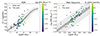 |
Fig. 1. Mass−metallicity relation (left panel) and star formation main sequence (right panel) of our galaxy sample (circles color-coded by SFR in the left panel and by gas-phase metallicity gradient in the right panel) in comparison with the distribution of SDSS galaxies and LVL galaxies. The solid or dashed lines represent the median trend or linear fit; the shaded regions indicate one and two standard deviations from the median trend. The metallicity is derived using N2S2Hα method (See Sect. 3.1 for details). |
As a comparison, in the left panel of the figure we also show the MZR of galaxies of Local Universe drawn from the SDSS-DR7 (Asplund et al. 2009). Emission-line fluxes of the SDSS galaxies are taken from the OSSY catalog 5 (Oh et al. 2011), and we require a S/N > 3 for all the emission lines used for metallicity estimates, as for our sample. As a result, we are left with about 110 000 galaxies. The metallicities of these SDSS galaxies are estimated with the same method as our sample galaxies. Instead of plotting the individual SDSS galaxies in Fig. 1, we calculated the median and standard deviation (with 3σ clipping) for galaxies falling into different logarithmic stellar mass bins from 108 to 1011 M⊙. In the low galaxy stellar mass end where the incompleteness of SDSS sample becomes significant, we performed a linear fitting to the median MZR of 108.2 to 109 M⊙ and extrapolated the best-fit relation down to 106.5 M⊙ in stellar mass. For the main sequence, we compare our measurements with the main sequence trends at z ∼ 0 from the local volume legacy (LVL) survey (Dale et al. 2023). We performed a linear fitting to their sample of stellar mass under 1010 M⊙. The comparison shown in Fig. 1 suggests that our sample galaxies largely follow the MZR and SFMS relation, with a possible exception for the few most massive galaxies (> 109 M⊙) that have systematically higher metallicities and SFR than the median trends.
3.2. Spatial distribution and radial profiles of metallicities
In this section, we present the resolved maps of gas-phase metallicity, SFR(Hα), and emission line velocities. The radial gradients of metallicity and SFR are listed in Table A.1.
As examples, the resolved maps and radial profiles of NGC 1796 and NGC 1705 are shown in Fig. 2. NGC 1796 is chosen as a typical galaxy in our sample with a clear negative metallicity gradient, while NGC 1705 serves as an example with no significant metallicity gradient.
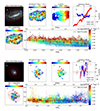 |
Fig. 2. Galaxies NGC 1796 and NGC 1705 as examples of our working sample. From top left to bottom right for each galaxy: three-color composite image (A) based on synthetic V, I, and R band images obtained from the MUSE cubes, overplotted with the isophotal ellipses of galaxy in a 0.2Re interval (the white ellipse represents 1Re); the Hα emission-line map (B) and its velocity field (C); the Hα velocity along the major or minor axis (D); the 12+log(O/H) map (E); and its distribution as a function of galactocentric radius (F). In panel F, the data points are color-coded by SFR, and the red triangles are the median values for each 0.2Re interval, with error bars denoting the standard deviation. The dashed line corresponds to the best-fit linear relation of the data points. Similar figures for the other galaxies in our sample can be found at https://github.com/Count-Lee/metallicity-gradient. |
NGC 1796 (upper panels of Fig. 2) has an obvious velocity gradient, suggesting a regular rotating disk. Subplot F of the upper panels of Fig. 2 suggests that, at a given radius, regions with higher SFR also tend to have higher metallicity. This positive correlation between SFR and metallicity at a small scale, is consistent with the result of Wang & Lilly (2021). They proposed that this reflects a changing star formation efficiency rather than a changing gas inflow rate. NGC 1705 (lower panels of Fig. 2) does not have an obvious Hα velocity gradient, suggesting a significant disturbance of the velocity field. We note that an irregular gaseous velocity field does not necessarily mean a lack of disk rotation, as the gas component can be easily disturbed by outflow and inflow activities. Unlike NGC 1796, there is no clear positive correlation between local SFR and metallicities in NGC 1705 (subplot E of the lower panel). This may reflect a stochastic spatial distribution of star formation activities or an efficient metal mixing in the galaxy.
Among our sample, 18 galaxies have a clear positive metallicity gradient, while the rest have either a negative or zero gradient. With a logarithmic median stellar mass of 8.36 (in M⊙), the median metallicity gradient of our sample is −0.021 ± 0.84, with a typical median uncertainty of 0.016 in unit of dex kpc−1, and −0.026 ± 0.092 with median uncertainty of 0.018 in unit of dex  . The median gradient is much shallower than typical high-mass galaxies. For example, a median gradient of −0.08 dex kpc−1 is found for MaNGA galaxies in the stellar mass range 9.0 < log(M⋆/M⊙) < 11.5 (Belfiore et al. 2017). It is our goal in this work to explore the physical drivers of the shallow or inverted metallicity gradients of dwarf galaxies.
3.3. Mass-metallicity gradient relation
The galaxy stellar mass−metallicity gradient relation of our dwarf galaxies is shown in Fig. 3. For comparison purposes, literature samples of low-mass galaxies (Ho et al. 2015; Bresolin 2019) and high-mass galaxies from MaNGA Pipe3D Value-added catalog (Sánchez-Menguiano et al. 2016) are also plotted. The MaNGA galaxies are presented as the gray-shaded region in Fig. 3. The Ho et al. (2015) sample includes metallicity gradients of galaxies in units of dex kpc−1 and dex  , covering a stellar mass range of 108 M⊙ to 1011 M⊙, with 21 galaxies below a stellar mass of 109.5 M⊙ and 14 galaxies below 109 M⊙. Their sample galaxies are represented as purple dots. Bresolin (2019) collects a sample of small and nearby spiral galaxies, and their metallicity gradients are based on long-slit spectroscopy of H II regions. Here we only plot the 8 galaxies (blue dots) with stellar mass lower than 109.5 M⊙ in their sample. We also include the metallicity gradients from the SAMI survey (Poggianti et al. 2017) for comparison. SAMI observed a number of low-mass galaxies and calculated their metallicity gradients in units of dex
  (Poetrodjojo et al. 2021). Here we only plot the median trend of SAMI results for clarity.
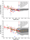 |
Fig. 3. Metallicity gradient vs. galaxy stellar mass relation, where the metallicity gradient is expressed in dex kpc−1 in the upper panel and in dex |

The upper panel of Fig. 3 shows the metallicity gradients in units of dex kpc−1, and the lower panel shows the gradients normalized to  . To aid in visualizing the mass-dependent behavior, we grouped our galaxies into five mass intervals (11 galaxies each) and calculated the median values and standard deviation of their metallicity gradients. The results are shown as green squares in Fig. 3. The median gradients decrease with increasing stellar mass across the mass range explored here, no matter how the gradients are quantified. To quantify the strength of the correlation, we calculated the Spearman’s rank correlation coefficient r. The derived r values are in the range of ∼−0.5 to −0.6 (Table 1), with the gradients normalized by Re having a more negative r (stronger negative correlation). This suggests a moderate correlation between the metallicity gradients and the stellar mass. The p-values are ≲10−5, far below the 0.05 threshold, rejecting the null hypothesis that the correlation arises by chance.
Linear fit and Spearman’s rank correlation test for the relationship between the metallicity gradient and other properties.
Given the limited sample size, we fit a simple linear relation between metallicity gradients and log(M⋆) for our sample:
![$$ \begin{aligned} \nabla _{r}[\mathrm{O} / \mathrm{H} ]= \alpha \log M_{\star }+ \beta . \end{aligned} $$](/articles/aa/full_html/2025/06/aa52978-24/aa52978-24-eq21.gif)
The best-fit linear relation is shown as red dashed line and the uncertainty is represented by the shaded region in Fig. 3). Our finding that the correlation becomes stronger when the radius is normalized by Re for dwarf galaxies aligns with previous studies of higher-mass galaxies (e.g., Belfiore et al. 2017; Sharda et al. 2021a).
The variation of metallicity gradient with stellar mass may be primarily driven either by a more significant drop of metallicity at smaller galactocentric radii or a relative enhancement of metallicity at larger radii. To explore this issue, we divided each galaxy into inner and outer regions using the 1/2 Re boundary and summed the emission line flux in these regions separately to calculate their metallicities. Given the general correlation between gas-phase metallicity and galaxy stellar mass (MZR), we removed a best-fit linear dependence of global metallicity on stellar mass for our galaxies and explored the correlation between residual metallicity and the metallicity gradient.
Figure 4 illustrates the relationship between residual metallicity and metallicity gradient for the inner and outer galaxy regions separately. A clear negative correlation exists between the metallicity gradient and residual metallicity for the inner regions, with a Spearman’s correlation coefficient of r ≃ −0.29. No correlation is observed between the residual metallicity of the outer galaxy regions and the metallicity gradient. This result suggests that the flattening of the metallicity gradient is primarily caused by a more significant drop of metallicity toward smaller galactic radii, rather than a relative enhancement of metallicity at larger radii.
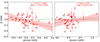 |
Fig. 4. Residual metallicity vs. metallicity gradient. Each circle presents one single galaxy in our sample, and the red shaded region represents 1σ uncertainties of the best-fit relation; the slope is shown as a red dashed line. In both panels the X-axis represents the metallicity residual of the inner region or outer region of the galaxy in the left or right panel, respectively. The results of best linear fit are shown in the upper right corner in each panel. |
3.4. Dependence of the metallicity gradient on secondary parameters
The spatial distribution of metallicities is in principle regulated by several factors, such as the in situ star formation (metal generation), turbulence driven metal mixing, and metallicity dilution induced by metal-poor gas inflow or metal-enriched gas outflow. As will become clear later, metallicity gradients have the strongest correlation with stellar mass. However, it is not clear what is the physical driver of the metallicity gradients in galaxies of different masses and what drives the substantial scatter of metallicity gradients at given stellar mass. In this section, we further explore the connection between metallicity gradients and other galaxy properties. To make a fair comparison of galaxies with different mass and size, we focus on exploring the metallicity gradients normalized by the effective radius Re. However, unless otherwise explicitly noted, the general conclusion in this paper is not affected by the way the metallicity gradient is expressed.
3.4.1. Dependence on the gaseous velocity field
We first classified our galaxies into two subsamples according to the regularity of the Hα velocity field. A regular velocity field means an overall velocity gradient along the photometric major axis across the main body of galaxies, which is presumably driven by disk rotation, whereas an irregular gaseous velocity field is most likely due to significant disturbance of the interstellar medium by either outflow or inflow activities. Our classification is based on a visual inspection of the Hα velocity field and the velocity variation along the major and minor axes, as exemplified in Fig. 2, which suffices for our purpose. It turns out that 33 galaxies exhibit a regular velocity field and the remaining 22 galaxies exhibit an irregular velocity field. We emphasize that the classification of regular and irregular gaseous velocity field serves as an indicator of the dynamical status of the interstellar medium (ISM), rather than the presence or lack of a galaxy disk.
In the left panel of Fig. 5, we show the stellar mass distributions of the two subsamples. It is clear that galaxies with a regular velocity field have a stellar mass range and distribution similar to those with an irregular velocity field in our sample. In the middle panel, we compared the metallicity gradient distribution of the two subsamples with or without a regular velocity field. Since metallicity gradients are correlated with galaxy stellar mass, we also explored the metallicity gradient difference of the two subsamples after removing the best-fit linear stellar mass dependence of the metallicity gradient.
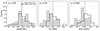 |
Fig. 5. Histogram of metallicity gradient distribution of galaxies with or without a regular velocity field. The right panel is for the distribution of residual metallicity gradient after removing the best-fit linear dependence on stellar mass. The gray filled histograms represent galaxies with a clear rotation velocity field, while the black open histograms represent galaxies without a regular gaseous rotational velocity field. The two dotted vertical lines in each panel represent the median values of the two subsamples, and the value in the upper left corner corresponds to the p-value from the Kolmogorov-Smirnov tests conducted between galaxies with or without a regular velocity field. |
The subsample with an irregular velocity field has a zero median metallicity gradient, and the subsample with a regular velocity field has a median gradient of −0.057 dex  . After controlling for stellar mass, the two subsamples still show systematically different distributions of metallicity gradients. Particularly, the galaxies with a regular velocity field have a median Δ(∇Re) of −0.009 dex
  , whereas it is 0.015 dex
  for those with an irregular gaseous velocity field. The Kolmogorov–Smirnov test suggests that the two subsamples are not likely to be drawn from the same underlying distribution (p-value = 0.004, D = 0.348). Nevertheless, we note that the mass-metallicity correlation shown in Fig. 3 remains virtually unchanged when galaxies with an irregular gaseous velocity fields are excluded.
Ma et al. (2017) invokes a toy model to explore the connection between metallicity gradient and disk regularity, which is updated by Sun et al. (2024). In their model, if the metals do not mix efficiently between radial annuli, the gas-phase metallicity follows the mass fraction of stars, resulting in a negative metallicity gradient. Galaxies with an irregular gaseous velocity field may be strongly perturbed by violent processes, such as mergers, rapid gas inflows, and strong feedback-driven outflows, which may substantially disturb pre-existing rotation-dominated velocity field and cause efficient gas re-distribution on galactic scales and thus leads to non-negative metallicity gradients. Galaxies with a regular rotational velocity field but flat metallicity gradients may be in a transition stage, e.g. during a significant gas inflow after which a negative metallicity gradient will build up at a later time.
For our sample of ordinary dwarf galaxies in the Local Universe, galaxy mergers and violent gas accretion are unlikely to play a significant role (see also Sect. 3.4.6). Instead, the irregular gaseous velocity field is most likely a result of stellar feedback disturbing the interstellar medium. Furthermore, the fact that the least massive galaxies in our sample predominantly exhibit positive metallicity gradients suggests that the above-mentioned transitional stage (if any) has a prolonged duty cycle for these galaxies.
3.4.2. Dependence on radial gradient of current star formation
According to the classical inside-out disk growth paradigm (e.g., Chiappini et al. 2001), gas accumulation and consumption (through star formation) are faster at smaller galactocentric radii, which would naturally predict a negative metallicity gradient if there is negligible radial migration of matter. In this paradigm, the star formation rate profile has a direct consequence on the metallicity gradient (e.g., Pilkington et al. 2012). In this section, we explored the connection of the radial gradients of metallicity and star formation.
Figure 6 shows the metallicity gradients as a function of the radial gradients of SFR surface density (left panel) and sSFR (right panel). The correlation with SFR surface density and sSFR radial gradients is very weak, with a Spearman’s rank correlation coefficient r of −0.13 and −0.11, and a p-value of 0.36 and 0.43, respectively. This strongly suggests that physical processes other than in situ star formation, such as metal mixing and migration or radially differential dilution of metallicity, play more important roles in shaping the metallicity gradients. The lack of correlation rules out the possibility that metal-poor gas inflow to galactic center drives the flat or positive metallicity gradient, as otherwise we would expect enhanced central star formation and thus steeper (i.e., more negative) radial gradient of SFR surface density in galaxies with flatter or more positive metallicity gradient.
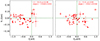 |
Fig. 6. Metallicity gradient vs. SFR and sSFR surface density gradients of our sample galaxies. The circles represent the galaxies measured in this work. The green dashed line represents when the gradient is 0. The Spearman correlation test is also given in the bottom right corner in each panel. |
3.4.3. Dependence on the baryonic mass
We investigated the correlation between the metallicity gradient and the total baryonic mass of our galaxies. Here the baryonic mass includes the stellar mass and cold interstellar gas mass (based on HI 21 cm emission line and star formation rate). We intend to explore which of the two (baryonic mass and stellar mass) has the strongest correlation with metallicity gradient.
We plot the result in Fig. 7. In this figure, we can see a negative correlation between the baryonic mass and the metallicity gradient. The slope of the best-fit linear relation is −0.089 ± 0.017, slightly lower than that between stellar mass and metallicity gradient in unit of dex  . The Spearman’s rank correlation coefficient r is −0.58 with 1σ uncertainties of 0.073. Although the correlation coefficient here is slightly higher than that with stellar mass, the difference is within the 1σ uncertainties.
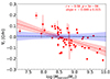 |
Fig. 7. Metallicity gradient as a function of the total baryonic mass. The red circles represent the galaxies measured in this work. The red dashed line and shaded region represent the best-fit linear relation and its 1σ uncertainties. The blue dashed line represents the best-fit linear relation between the residual metallicity gradient (after removing the stellar mass dependence) and the baryonic mass, and the blue shaded region represents 1σ uncertainties of the best-fit relation, with the slope shown in blue. The green horizontal dashed line marks a metallicity gradient of 0. |
Furthermore, we also explored the residual metallicity gradient correlation with baryonic mass by removing the best-fit linear dependence of the radient on stellar mass (Sect. 3.3). Specifically, for each galaxy, we derived the deviation Δ(∇Re) of its metallicity gradient from the best-fit relation and perform a linear fitting of the residual gradient vs. baryonic mass. The best-fit linear relation is overplotted (in blue color) in Fig. 7. We find that the Spearman’s rank correlation coefficient r is −0.046, and the best-fit slope is 0.011 ± 0.022. So there is virtually no correlation between metallicity gradient and baryonic mass, once the stellar mass dependence is removed.
To further examine the lack of intrinsic correlation between baryonic mass and metallicity gradients, we calculated the partial correlation coefficient between metallicity gradients and gas mass while controlling for stellar mass. The resulting r is −0.093, indicating no intrinsic correlation between the gas mass and the metallicity gradients. Above all, stellar mass is the driver of the apparent correlation between metallicity gradients and baryonic mass.
3.4.4. Dependence on effective yield
As mentioned in Sect. 2.9, the effective yield yeff serves as a diagnostic parameter for probing outflows or gas inflows. Here we explored the connection between yeff and metallicity gradients, in an attempt to probe the relevance of inflow and outflow. While yeff has been routinely estimated in the literature, we emphasize that the fundamental assumption of instantaneous and homogeneous chemical mixing for deriving yeff is often violated in reality, as evidenced by the metallicity gradients and differential spatial distributions of gas and stars commonly observed in galaxies. Nevertheless, a galaxy operates as an interconnected ecosystem, where gas inflows and outflows facilitate exchange between the inner and outer regions. Therefore, a global yeff still provides helpful insights into the overall baryon cycling process.
In Fig. 8, the upper two panels show the distribution of our galaxies on yeff vs. stellar mass and yeff vs. baryonic mass planes. The true stellar yield derived by Pilyugin et al. (2007) is overplotted as a reference (horizontal green dashed lines in Fig. 8). The best-fit relation between yeff and baryonic mass from Tremonti et al. (2004) is also overplotted for comparison. Most of our galaxies (40 in 55) have lower yeff than the true stellar yield, which hints at a significant influence by gas outflow or inflow. yeff has no correlation with stellar mass (r ≃ 0.1) but has a moderate correlation with the baryonic mass (r ≃ 0.4). A correlation between yeff and baryonic mass has already been found by Tremonti et al. (2004). If assuming baryonic mass is a better tracer of the total galaxy mass than stellar mass (as evidenced by the existence of a tight baryonic Tully−Fisher relation; McGaugh 2012), the correlation may imply a connection between gravitational potential well and yeff, and thus may support the scenario of metal-enriched outflow driving lower yeff, because shallower potential well in lower-mass galaxies favors a stronger stellar feedback driven outflow. It is however intriguing that van Zee & Haynes (2006) did not find a correlation of yeff with dynamical mass for their sample of (mainly) low-mass galaxies.
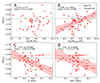 |
Fig. 8. Panels A, B, C, and D show the relation between effective yield and stellar mass, total baryonic mass (stellar+neutral atomic mass), metallicity gradient and residual metallicity gradient (after removing the stellar mass dependence). In each panel the green dashed horizontal line represents the true stellar oxygen yield derived by Pilyugin et al. (2007), and the red dashed line and the shaded region are the best-fit linear relation and its 1σ uncertainties. The Spearman’s rank correlation coefficient r, p-value and the best-fit slope are given in the upper left corner of each panel. In panel B we also plot the best-fit relation from Tremonti et al. (2004). |
The lower two panels of Fig. 8 show the relation between yeff and metallicity gradients of our galaxies. Particularly, in the lower right panel, the stellar mass dependence of metallicity gradient has been removed as in previous section. As indicated in the lower panels, the metallicity gradient shows a moderate (r ≃ 0.4) and significant (p-values < 0.01) negative correlation with yeff. It appears that the metallicity gradient shows a slightly stronger correlation with yeff once controlling for galaxy stellar mass. Therefore, yeff partially explains the scatter of the galaxy stellar mass−metallicity gradient correlation. We will revisit this point later in the paper.
3.4.5. Dependence on stellar gravitational potential
M⋆/Re has been often used as a proxy for galaxy stellar potential well in the literature (e.g., Sánchez-Menguiano et al. 2024). Here we explored the relation between M⋆/Re and metallicity gradients of our galaxies. In addition, we also explored the connection with the radial slope of the stellar mass surface density profile. The results are shown in Fig. 9. The metallicity gradient has a moderate negative correlation with log(M⋆/Re), but no correlation with the stellar mass surface density gradient. Nevertheless, once controlling for the galaxy stellar mass dependence, the correlation with log(M⋆/Re) disappears.
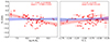 |
Fig. 9. Dependence of metallicity gradient on stellar gravitational potential, as represented by M⋆/Re, and radial gradient of the stellar mass surface density. The meanings of the different lines and colors are similar to those in Fig. 7. The apparent correlation of metallicity gradients with M⋆/Re or stellar mass surface density disappears once the dependence on stellar mass is removed. |
3.4.6. Dependence on environment
Both local and large-scale environment may affect the metallicity distribution in galaxies. For instance, ram pressure or tidal disruption and compression in group and cluster environment may cut off cosmic gas accretion, change the spatial distribution of gas inside galaxies and thus affect the star formation distribution and metallicity distribution (e.g., Lara-López et al. 2022; Williamson et al. 2017); There is also evidence of disturbed gaseous disk in close pairs of galaxies, suggesting the influence of local environment on metallicity distribution. In this subsection, we explored the environmental dependence of the metallicity gradients. Specifically, for the large-scale environment, we divided the whole sample into two environmental types: field galaxies (26) and cluster galaxies (29), where galaxies located in groups and clusters are both referred as cluster galaxies for brevity. And for the local environment, following Argudo-Fernández et al. (2015), we define the projected galaxy number density parameter as
where ηk is the projected physical distance to the k-th nearest neighbor. Here, we adopt 5 as the value of k. The farther the kth nearest neighbor, the lower the projected number density ηk.
The comparison of metallicity, metallicity gradient, and metallicity gradient residual distributions of field and cluster galaxies is shown in Fig. 10. The open histograms in Fig. 10 represent the distributions of field galaxies, while the gray filled histograms represent the cluster galaxies. From the metallicity distributions (left panel), we see a median metallicity difference between the field and cluster galaxies, which is probably attributed to the inhomogeneous nature of the current sample. In addition, compared to the field galaxies, the median metallicity gradient (middle panel) of cluster galaxies is slightly more negative than field galaxies. In order to alleviate the effect of mismatch between the mass and metallicity distributions of our field and cluster subsamples, we subtracted the best-fit stellar mass−metallicity gradient linear relation from the measured metallicity gradient, and presented the metallicity gradient residual distribution in the right panel of Fig. 10. The field and cluster galaxies have virtually the same median metallicity gradient residual (∼−0.01). To further quantify the difference or similarity of the gradient residual distributions of the two subsamples, we run a Kolmogorov–Smirnov test for a null hypothesis that the two are drawn from the same underlying distribution, and find a p-value of 0.89, which means that the two subsamples are consistent with being drawn from the same underlying distribution. Therefore, the large-scale environment appears not relevant in shaping the metallicity gradient of these galaxies.
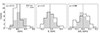 |
Fig. 10. Environmental dependence of the metallicity, metallicity gradient and metallicity gradient residual (obtained by removing the best-fit linear relation between gradient and stellar mass) distributions. The gray shaded histograms represent the cluster subsample, and the open histograms represent the field subsample. The vertical black (gray) dashed line marks the median values of field (cluster) subsample. The value in the upper left corner corresponds to the p-value from the Kolmogorov-Smirnov tests conducted between galaxies in different environments. |
In Fig. 11, we plot the metallicity gradients as a function of projected galaxy number density. We find no significant correlation between metallicity gradient and projected galaxy number density, with a Spearman’s rank correlation coefficient r = −0.065 and p-value = 0.65. This implies that the local environment also does not affect the metallicity gradient of our galaxies.
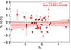 |
Fig. 11. Metallicity gradients as a function of the projected local number density of galaxies. Circles represent individual galaxies, and the red shaded region represents 1σ uncertainties of the best-fit relation. The slope is shown as a red dashed line. The Spearman correlation coefficient and best-fit slope are given in the upper right corner. |
3.5. Partial correlation analysis and a combination of stellar mass and yeff
In the previous subsections, we have explored the connection between metallicity gradients and various galaxy parameters. Here we summarize the strength of these connections by presenting the Spearman partial correlation coefficients (PCC; controlling for galaxy stellar mass) in Fig. 12. The galaxy parameters that we have considered include the effective yield, yeff, baryonic mass, logarithmic stellar gravitational potential log(M⋆/Re), radial gradients of stellar mass surface densities, star formation surface densities and sSFR. In Fig. 12, the error bars of the PCC are uncertainties obtained by bootstrap sampling of our galaxy sample.
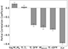 |
Fig. 12. Partial correlation coefficients between metallicity gradients and various parameters by controlling for galaxy stellar mass, M⋆. The filled bars show the Spearman’s rank correlation coefficient, and the uncertainties are computed via bootstrap random sampling. |
As can be seen, after controlling for galaxy stellar mass, yeff is the most important and dominant galaxy parameter in predicting the metallicity gradient of a galaxy, and the second most relevant parameter is the baryonic mass. The PCC analysis indicates that the metallicity gradients have a moderate correlation (r ≃ 0.4) with yeff, whereas the other secondary parameters have a much weaker correlation (r ≲ 0.2).
Now that we know that effective yield is the second most relevant parameter that correlate with metallicity gradient, we performed a linear least-squares fitting of metallicity gradient as a function of a combination of logarithmic stellar mass and effective yield, i.e.,
![$$ \begin{aligned} \nabla _{r}[\mathrm{O} / \mathrm{H} ] = \alpha \times f(M_{\star },y_{\rm eff})+\beta , \end{aligned} $$](/articles/aa/full_html/2025/06/aa52978-24/aa52978-24-eq27.gif)
where f(M⋆, yeff) is a linear combination of logarithmic stellar mass and effective yield, defined as
To search for the optimal parameter values of α, β, and γ, we traversed the γ values (accurate to two decimal places), and for each γ, performed a linear least-squares fitting to our galaxies and find α and β values that minimize the scatter of ∇r[O/H] around the best-fit linear relation (Eq. (10)). From this iterative linear least-squares fitting, we find that the optimal parameter values of α, β, and γ are −0.091 ± 0.013, 0.45 ± 0.17, and 1.15.
We note that the above best-fit α coefficient value is equal to that of the linear relation of ∇r[O/H] vs. log M⋆/M⊙-pagination
(Sect. 3.3), but the Spearman’s rank correlation coefficient with ∇r[O/H] increases from ∼ − 0.58 to −0.67. The scatter of ∇r[O/H] around the best-fit relations is reduced from 0.068 to 0.060 after involving log yeff. The mean measurement uncertainty of metallicity gradient is 0.006 dex  . Therefore, log yeff accounts for 22% (1−(0.0602 − 0.0062)/(0.0682 − 0.0062)) of the scatter of ∇r[O/H] −stellar mass relation. Figure 13 shows the distribution of our galaxies on the ∇r[O/H] vs. (log M⋆/M⊙ + 1.15 × log yeff) plane.
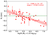 |
Fig. 13. Relation between metallicity gradients and μ1.15 = log M⋆/M⊙ + 1.15 × log yeff. The coefficient of log yeff, α = 1.15, minimizes the scatter of metallicity gradients at given μ1.15. The best-fit slope, Spearman’s rank correlation r and p-value are given in the upper right corner of this figure. The red dashed line and shaded region represent the best-fit linear relation and its 1σ uncertainties. The combination parameter μ1.15 exhibits a strong correlation with metallicity gradients, and represents the tightest correlation observed with metallicity gradients (see Sect. 3.5 for details). |
4. Discussion
With the connection between metallicity radial profiles and other galaxy properties explored in the previous section, we here compare our results with previous studies and discuss the possible implications of these results on dwarf galaxy evolution.
4.1. Mass-metallicity gradient relation at the low-mass end
According to previous studies (e.g., Zaritsky et al. 1994; Wang & Lilly 2022; Wang et al. 2024), the well-known exponential disks and negative radial gradients of gas-phase metallicity in massive disk galaxies are the result of inside-out star formation or gradual gas-flow along the disk from outside in. The former scenario suggests that the presence of the exponential disk is a natural result of galaxy star formation regulated by gas distribution in galaxies, with the inner high gas density regions forming stars earlier and more efficiently than the outer disks. A negative metallicity gradient follows naturally in this inside-out disk formation process. The gas-flow scenario attributes the negative metallicity gradients to a gradual metal enrichment of gas that flows from outside in. These two scenarios are not necessarily mutually exclusive, and both may occur in real galaxies.
Physical drivers of the metallicity gradient can be constrained by exploring its connection with various galaxy properties. Data from several large IFU surveys have been used to identify the mass−metallicity gradient relation (MZGR) in a number of studies (MaNGA, e.g., Belfiore et al. 2017; SAMI, e.g., Poetrodjojo et al. 2021). These studies found that, starting from the low galaxy stellar mass end of their samples (log(M⋆/M⊙)∼9), the metallicity gradient gradually becomes more negative, with the trend showing a mild curvature around log(M⋆/M⊙)∼10 − 10.5. At the higher-mass end (log(M⋆/M⊙) > 11), the metallicity gradients flatten again. We note that the metallicity gradient variation with galaxy mass is found to be generally weak, with no mass dependence found in some studies (e.g., Lian et al. 2018). For the higher-mass end, the general view is that the flattening of the metallicity gradient can be ascribed to the general behavior of evolved systems to reach an equilibrium abundance at late times. In this scenario, as galaxy grows, the stellar mass increases, and the flattening should occur inside-out, with central regions reaching their equilibrium metallicity earlier and having lower gas fraction than do the outer regions (e.g., Belfiore et al. 2017; Pilyugin & Tautvaišienė 2024).
However, for dwarf galaxies (log(M⋆/M⊙) ≲ 9.5), we found that the situation appears quite different. The metallicity gradients become gradually less negative (i.e., flatter or more positive) toward the lower-mass end of dwarf galaxies. Instead of being attributed to a progressive saturation of metal production with radius as mentioned above for massive galaxies, the finding for dwarf galaxies is more likely due to a more significant metal mixing and transport within lower-mass dwarf galaxies. As shown in Sect. 3.4.1, galaxies with irregular gaseous velocity fields tend to have less negative or more positive metallicity gradients. The irregular gaseous velocity field suggests significant perturbations in the galaxy-scale distribution of the interstellar medium (ISM), potentially driving the redistribution of metals, primarily from the inner regions outward. This is supported by the greater degree of metallicity suppression observed in the central regions compared to the outskirts of our galaxies toward the lower-mass end (Fig. 4). We note that radial mixing of metals has also been invoked to explain the shallower metallicity gradients of older stellar populations of Milky Way-like galaxies (e.g., Graf et al. 2024).
4.2. Stellar feedback as an important factor reshaping metallicity distribution
Understanding how gas flows and recycles is crucial in studying galaxy evolution. Gas inflow is generally challenging to identify in observations. While gas outflows have been identified in numerous studies, the overall significance of their impact on baryonic cycling within galaxies is unclear. In this section, we discuss how gas flow influences metallicity gradients, based on the analysis in Sect. 3.4.
We first consider the inflow of metal-poor gas. If the infalling gas is relatively metal-poor, it dilutes the gas enriched by in situ star formation, thereby reduces metallicity, and at the same time may enhance local star formation activities. This may therefore lead to an anti-correlation between metallicity and star formation rate (SFR) if gas inflow dominates. However, as exemplified by the two galaxies NGC 1796 and NGC 1705 (Sect. 3.2), we do not find such negative correlation between metallicity and SFR in most star-forming regions in our sample, and only few regions in galaxies such as NGC 1705 (a starburst dwarf; at 1Re radius) exhibit high SFR and low metallicity. Our sample’s scarcity of such anti-correlation between SFR and metallicity indicates that metal-poor gas inflow may not be the dominant factor in dwarf galaxies and contributes little to the metallicity gradients in general.
The lack of correlation with SFR and specific SFR (sSFR) surface density gradients (Sect. 3.4.2) again supports our point of view. If we assume that metal-poor gas inflow is the dominant factor (as compared to metal-enrichment outflow) in dwarf galaxies leading to inverted metallicity gradients, we expect steeper SFR and sSFR surface density gradients where the metallicity gradient is flatter. However, as demonstrated in Fig. 6, we did not find a strong correlation between these two gradients, suggesting that the inflow scenario may not be the dominant factor shaping metallicity distribution in most dwarf galaxies.
Besides gas inflow, other processes, such as metal-enriched gas outflow, turbulence-driven spatial mixing, may also affect the metallicity distribution within galaxies. In this regard, one commonly mentioned scenario is the so-called “galactic fountains”, where metal-enriched gas outflow launched (by stellar feedback) from smaller galactocentric radii is finally deposited at larger radii. (e.g., Gibson et al. 2013; Ma et al. 2017; Tissera et al. 2022).
Previous studies (e.g., Tremonti et al. 2004; Daddi et al. 2007; Lara-López et al. 2019) suggest that metal-enriched outflow is the primary factor that results in the observed lower effective yield of metals yeff in galaxies of lower baryonic mass. Therefore, yeff may serve as an indicator of outflow efficiency. We find a significant correlation between metallicity gradient and yeff, even after controlling for galaxy mass. This suggests that metal-enriched outflow is indeed an important mechanism in re-distributing metals in dwarf galaxies.
Regarding outflow, we also explore the correlation between stellar gravitational potential, baryonic mass and metallicity gradient. In principle, feedback-driven outflow is expected to be more efficient in galaxies with shallower gravitational well. While the finding that these parameters (log(M⋆/Re), Mbaryon) have a significant correlation (r ∼ −0.4–−0.6) with metallicity gradient may suggests a non-negligible role the gravitational potential well in (re)shaping metallicity gradient. it is however intriguing that the correlations disappear after controlling for galaxy stellar mass. This indicates a non-trivial connection between stellar feedback and metallicity distribution. The effective yield correlates with metallicity gradient, but it only accounts for 22% of the scatter of MZGR. We speculate that outflow is probably just one way that feedback affects metallicity distribution. Other metal mixing and transport process, such as feedback-fed turbulence of ISM, may also play important roles.
Some studies attributed lower oxygen abundance at the centers of some dwarf galaxies to pristine gas infall rather than metal-enriched outflow (e.g., Kewley et al. 2010; Chung et al. 2023). This may be in line with our finding of a greater degree of suppression of metallicities toward smaller galactic radii of lower-mass galaxies (Fig. 4). Gas inflow may be important in some dwarf galaxies, especially the starburst ones (e.g., Tang et al. 2022), but it may not be a dominant factor that determines gas metallicity gradient of dwarf galaxies in general.
4.3. The relevance of environment
Environment can have a significant impact on galaxy evolution. Galaxies in clusters tend to have higher metallicities than field galaxies (e.g., Ellison et al. 2009; Lian et al. 2019). However, studies of the effect of environment on gas metallicity gradients have so far been rather limited. While some studies find that the metallicity gradient is independent with the density of the environment (e.g., Sánchez-Menguiano et al. 2018), others find galaxies in clusters tend to have flatter metallicity gradients than field galaxies (e.g., Kewley et al. 2010; Lara-López et al. 2022; Franchetto et al. 2021).
In this work, we find that field galaxies have a significantly lower metallicity than cluster galaxies, consistent with previous results. However, their metallicity gradients exhibit negligible differences when controlling the stellar mass. Moreover, we find no significant correlation between metallicity gradient and the projected local galaxy number density. These results may imply that gas accretion from intergalactic medium (IGM) or circumgalactic medium (CGM), if any, may influence overall metallicities, but it is not directly connected to the metallicity distribution within dwarf galaxies. Due to their shallow potential wells, dwarf galaxies are expected to be advection-dominated rather than governed by cosmological accretion (Sharda et al. 2021b). This means that internal metal redistribution processes are more important than external gas accretion in shaping the radial profile of metallicity in dwarf galaxies.
5. Summary
In this paper, we presented a study of the radial gradients of gaseous metallicities of a sample of nearby dwarf galaxies, that span a stellar mass range of ∼107 to 109.5 M⊙ and based on MUSE wide-field mode spectroscopic observations. These galaxies are representative of ordinary star-forming dwarf galaxies in the Local Universe, in the sense that they follow the general stellar mass−metallicity relation and the star-forming main sequence relation. The metallicity gradients are compared with various galaxy properties, including stellar mass, gaseous velocity field regularity, effective yield of metals, baryonic mass, star formation rate surface density and specific star formation rate gradient, stellar gravitational potential, and global-local environment, in order to probe the primary physical drivers of the metallicity distribution of dwarf galaxies. Our main results are summarized as follows:
-
We find a significantly negative MZGR, with a best-fit slope of −0.091 ± 0.017 dex
 , and a Spearman’s rank correlation coefficient of −0.56 ± 0.081. The mass-dependent metallicity gradient variation is primarily driven by a higher degree of metallicity depression in the central regions of lower-mass galaxies. The MZGR found here is in remarkable contrast with a lack of (e.g., Lian et al. 2018) or mildly positive galaxy mass dependence of gas-phase metallicity gradient found for high-mass galaxies (> 109 M⊙; e.g., Belfiore et al. 2017). This mass-dependent MZGR reflects the interplay of physical processes related to metal production (in situ star formation), metal redistribution (driven by feedback, outflow or turbulence) and metallicity dilution (metal-poor gas inflow), as suggested by recent models (e.g., Sharda et al. 2024).
 -
Except for the primary dependence on stellar mass, and the secondary relevant properties of gaseous velocity field regularity and effective yield (see below), all the other properties explored here have no residual correlation with metallicity gradients after controlling for stellar mass. The lack of correlation with star formation indicates that metal distribution produced by in situ star formation is subject to substantial modulation by redistribution processes.
-
Galaxies with an irregular gaseous velocity field are characterized by significantly disturbed ISM by stellar feedback or inflow, and are more likely to have positive metallicity gradient than those with regular velocity field, even after controlling for galaxy stellar mass. Since a negative metallicity gradient is a natural outcome from an inside-out galaxy formation process, the tendency indicates that kinematic disturbance in the ISM is accompanied by significant metal redistribution.
-
The effective yield of metals yeff shows a significant, albeit moderate, negative correlation with metallicity gradient, even after controlling for galaxy stellar mass: a partial correlation coefficient of ∼0.4. yeff accounts for 22% of the scatter of MZGR. Moreover, a linear combination of logarithmic stellar mass and effective yield significantly enhances the correlation with metallicity gradients compared to stellar mass alone, with a correlation coefficient r = −0.68. This suggests that stellar feedback-driven outflow (as a favored explanation of the low effective yield in dwarf galaxies) plays an important role in shaping the metallicity distribution within dwarf galaxies. The above-mentioned lack of correlation with baryonic mass and stellar gravitational well indicates that feedback-driven outflow, which presumably has a more profound effect on lower-mass galaxies, is not the only mechanism that directly re-shapes the metallicity distribution.
Positive (i.e., inverted) metallicity gradients have also been found recently for several low-mass galaxies at redshift ≳2, using slitless spectroscopy (e.g., Wang et al. 2019, 2020, 2022). These high-redshift dwarf galaxies have a stellar mass that falls at the high-mass end of our sample, where most nearby galaxies have negative gradients, and they are different from the local galaxies in the sense that they have ∼1 − 2 orders of magnitude higher star formation rate (density), and are presumably experiencing much more significant gas accretion from the cosmic web or local environment. In high-redshift dwarf galaxies, the much stronger star formation results in more efficient stellar feedback-driven metallicity redistribution. However, in the local dwarf galaxies at lower-mass, the generally inefficient and sporadic nature of star formation activities means that, in addition to stellar feedback-driven direct metal transport, other longer-term metal mixing processes, such as advection and diffusion, also play important roles in building up the metallicity distribution.
Acknowledgments
We acknowledge support from the National Key Research and Development Program of China (grant No. 2023YFA1608100), and from the NSFC grant (Nos. 12122303, 11973039, 11421303, 11973038, 12233008), FONDECYT Iniciación en investigación 2020 Project 11200263 and the ANID BASAL project FB210003. This work is also supported by the China Manned Space Project (Nos.CMS-CSST-2021-B02, CMS-CSST-2021-A07). We acknowledge support from the CAS Pioneer Hundred Talents Program, the Strategic Priority Research Program of Chinese Academy of Sciences (Grant No. XDB 41000000) and the Cyrus Chun Ying Tang Foundations.
References
- Argudo-Fernández, M., Verley, S., Bergond, G., et al. 2015, A&A, 578, A110 [NASA ADS] [CrossRef] [EDP Sciences] [Google Scholar]
- Asplund, M., Grevesse, N., Sauval, A. J., & Scott, P. 2009, ARA&A, 47, 481 [NASA ADS] [CrossRef] [Google Scholar]
- Bacon, R., Accardo, M., Adjali, L., et al. 2010, in Ground-based and Airborne Instrumentation for Astronomy III, eds. I. S. McLean, S. K. Ramsay, & H. Takami, SPIE Conf. Ser., 7735, 773508 [Google Scholar]
- Baldwin, J. A., Phillips, M. M., & Terlevich, R. 1981, PASP, 93, 5 [Google Scholar]
- Belfiore, F., Maiolino, R., Tremonti, C., et al. 2017, MNRAS, 469, 151 [Google Scholar]
- Bradley, L., Sipőcz, B., Robitaille, T., et al. 2024, astropy/photutils: 1.13.0 [Google Scholar]
- Bresolin, F. 2019, MNRAS, 488, 3826 [NASA ADS] [Google Scholar]
- Bryant, J. J., Owers, M. S., Robotham, A. S. G., et al. 2015, MNRAS, 447, 2857 [Google Scholar]
- Bulichi, T.-E., Fahrion, K., Mernier, F., et al. 2023, A&A, 679, A98 [NASA ADS] [CrossRef] [EDP Sciences] [Google Scholar]
- Bundy, K., Bershady, M. A., Law, D. R., et al. 2015, ApJ, 798, 7 [Google Scholar]
- Cappellari, M. 2017, MNRAS, 466, 798 [Google Scholar]
- Cappellari, M., & Copin, Y. 2003, MNRAS, 342, 345 [Google Scholar]
- Cardelli, J. A., Clayton, G. C., & Mathis, J. S. 1989, ApJ, 345, 245 [Google Scholar]
- Chiappini, C., Matteucci, F., & Romano, D. 2001, ApJ, 554, 1044 [NASA ADS] [CrossRef] [Google Scholar]
- Chung, J., Lee, J. H., Jeong, H., & Kim, S. 2023, ApJ, 949, 80 [Google Scholar]
- Courtois, H. M., Tully, R. B., Fisher, J. R., et al. 2009, AJ, 138, 1938 [Google Scholar]
- Croxall, K. V., van Zee, L., Lee, H., et al. 2009, ApJ, 705, 723 [NASA ADS] [CrossRef] [Google Scholar]
- Daddi, E., Dickinson, M., Morrison, G., et al. 2007, ApJ, 670, 156 [NASA ADS] [CrossRef] [Google Scholar]
- Dale, D. A., Boquien, M., Turner, J. A., et al. 2023, AJ, 165, 260 [Google Scholar]
- Dopita, M. A., Kewley, L. J., Sutherland, R. S., & Nicholls, D. C. 2016, Ap&SS, 361, 61 [NASA ADS] [CrossRef] [Google Scholar]
- Easeman, B., Schady, P., Wuyts, S., & Yates, R. M. 2024, MNRAS, 527, 5484 [Google Scholar]
- Ellison, S. L., Simard, L., Cowan, N. B., et al. 2009, MNRAS, 396, 1257 [NASA ADS] [CrossRef] [Google Scholar]
- Finlator, K., & Davé, R. 2008, MNRAS, 385, 2181 [NASA ADS] [CrossRef] [Google Scholar]
- Franchetto, A., Mingozzi, M., Poggianti, B. M., et al. 2021, ApJ, 923, 28 [NASA ADS] [CrossRef] [Google Scholar]
- Freudling, W., Romaniello, M., Bramich, D. M., et al. 2013, A&A, 559, A96 [NASA ADS] [CrossRef] [EDP Sciences] [Google Scholar]
- Gibson, B. K., Pilkington, K., Brook, C. B., Stinson, G. S., & Bailin, J. 2013, A&A, 554, A47 [CrossRef] [EDP Sciences] [Google Scholar]
- Graf, R. L., Wetzel, A., Bailin, J., & Orr, M. E. 2024, ApJ, submitted, [arXiv:2410.21377] [Google Scholar]
- Haynes, M. P., Giovanelli, R., Kent, B. R., et al. 2018, ApJ, 861, 49 [Google Scholar]
- Hemler, Z. S., Torrey, P., Qi, J., et al. 2021, MNRAS, 506, 3024 [NASA ADS] [CrossRef] [Google Scholar]
- Ho, I. T., Kudritzki, R.-P., Kewley, L. J., et al. 2015, MNRAS, 448, 2030 [NASA ADS] [CrossRef] [Google Scholar]
- Hummer, D. G., & Storey, P. J. 1987, MNRAS, 224, 801 [NASA ADS] [CrossRef] [Google Scholar]
- Hunter, D. A., & Hoffman, L. 1999, AJ, 117, 2789 [NASA ADS] [CrossRef] [Google Scholar]
- Kauffmann, G., Heckman, T. M., Tremonti, C., et al. 2003, MNRAS, 346, 1055 [Google Scholar]
- Kennicutt, R. C., Jr 1998, ARA&A, 36, 189 [NASA ADS] [CrossRef] [Google Scholar]
- Kewley, L. J., Rupke, D., Zahid, H. J., Geller, M. J., & Barton, E. J. 2010, ApJ, 721, L48 [NASA ADS] [CrossRef] [Google Scholar]
- Kourkchi, E., & Tully, R. B. 2017, ApJ, 843, 16 [NASA ADS] [CrossRef] [Google Scholar]
- Kreckel, K., Ho, I. T., Blanc, G. A., et al. 2019, ApJ, 887, 80 [NASA ADS] [CrossRef] [Google Scholar]
- Kudritzki, R.-P., Ho, I. T., Schruba, A., et al. 2015, MNRAS, 450, 342 [NASA ADS] [CrossRef] [Google Scholar]
- Lara-López, M. A., De Rossi, M. E., Pilyugin, L. S., et al. 2019, MNRAS, 490, 868 [CrossRef] [Google Scholar]
- Lara-López, M. A., Galán-de Anta, P. M., Sarzi, M., et al. 2022, A&A, 660, A105 [NASA ADS] [CrossRef] [EDP Sciences] [Google Scholar]
- Lee, H., Zucker, D. B., & Grebel, E. K. 2007, MNRAS, 376, 820 [Google Scholar]
- Lequeux, J., Peimbert, M., Rayo, J. F., Serrano, A., & Torres-Peimbert, S. 1979, A&A, 80, 155 [Google Scholar]
- Li, M., Cai, Z., Bian, F., et al. 2023, ApJ, 955, L18 [CrossRef] [Google Scholar]
- Li, X., Shi, Y., Bian, F., et al. 2025, ApJS, submitted, [arXiv:2501.04943] [Google Scholar]
- Lian, J., Thomas, D., Maraston, C., et al. 2018, MNRAS, 476, 3883 [NASA ADS] [CrossRef] [Google Scholar]
- Lian, J., Thomas, D., Li, C., et al. 2019, MNRAS, 489, 1436 [NASA ADS] [CrossRef] [Google Scholar]
- Loni, A., Serra, P., Kleiner, D., et al. 2021, A&A, 648, A31 [NASA ADS] [CrossRef] [EDP Sciences] [Google Scholar]
- Ma, X., Hopkins, P. F., Feldmann, R., et al. 2017, MNRAS, 466, 4780 [Google Scholar]
- Mannucci, F., Cresci, G., Maiolino, R., Marconi, A., & Gnerucci, A. 2010, MNRAS, 408, 2115 [NASA ADS] [CrossRef] [Google Scholar]
- Marasco, A., Belfiore, F., Cresci, G., et al. 2023, A&A, 670, A92 [NASA ADS] [CrossRef] [EDP Sciences] [Google Scholar]
- Marino, R. A., Rosales-Ortega, F. F., Sánchez, S. F., et al. 2013, A&A, 559, A114 [NASA ADS] [CrossRef] [EDP Sciences] [Google Scholar]
- McGaugh, S. S. 2012, AJ, 143, 40 [Google Scholar]
- Meyer, M. J., Zwaan, M. A., Webster, R. L., et al. 2004, MNRAS, 350, 1195 [Google Scholar]
- Oh, K., Sarzi, M., Schawinski, K., & Yi, S. K. 2011, ApJS, 195, 13 [NASA ADS] [CrossRef] [Google Scholar]
- Pagel, B. E. J., Edmunds, M. G., Fosbury, R. A. E., & Webster, B. L. 1978, MNRAS, 184, 569 [NASA ADS] [Google Scholar]
- Peng, Y.-J., & Maiolino, R. 2014, MNRAS, 443, 3643 [NASA ADS] [CrossRef] [Google Scholar]
- Pilkington, K., Few, C. G., Gibson, B. K., et al. 2012, A&A, 540, A56 [NASA ADS] [CrossRef] [EDP Sciences] [Google Scholar]
- Pilyugin, L. S., & Grebel, E. K. 2016, MNRAS, 457, 3678 [NASA ADS] [CrossRef] [Google Scholar]
- Pilyugin, L. S., & Tautvaišienė, G. 2024, A&A, 682, A41 [NASA ADS] [CrossRef] [EDP Sciences] [Google Scholar]
- Pilyugin, L. S., Thuan, T. X., & Vílchez, J. M. 2007, MNRAS, 376, 353 [NASA ADS] [CrossRef] [Google Scholar]
- Pilyugin, L. S., Grebel, E. K., & Kniazev, A. Y. 2014, AJ, 147, 131 [NASA ADS] [CrossRef] [Google Scholar]
- Pilyugin, L. S., Grebel, E. K., & Zinchenko, I. A. 2015, MNRAS, 450, 3254 [CrossRef] [Google Scholar]
- Poetrodjojo, H., Groves, B., Kewley, L. J., et al. 2021, MNRAS, 502, 3357 [NASA ADS] [CrossRef] [Google Scholar]
- Poggianti, B. M., Moretti, A., Gullieuszik, M., et al. 2017, ApJ, 844, 48 [Google Scholar]
- Raj, M. A., Iodice, E., Napolitano, N. R., et al. 2019, A&A, 628, A4 [NASA ADS] [CrossRef] [EDP Sciences] [Google Scholar]
- Roy, J.-R., Belley, J., Dutil, Y., & Martin, P. 1996, ApJ, 460, 284 [Google Scholar]
- Roychowdhury, S., Chengalur, J. N., Karachentsev, I. D., & Kaisina, E. I. 2013, MNRAS, 436, L104 [CrossRef] [Google Scholar]
- Sánchez, S. F., Lugo-Aranda, A. Z., Sánchez Almeida, J., et al. 2024, A&A, 682, A71 [NASA ADS] [CrossRef] [EDP Sciences] [Google Scholar]
- Sánchez-Menguiano, L., Sánchez, S. F., Pérez, I., et al. 2016, A&A, 587, A70 [NASA ADS] [CrossRef] [EDP Sciences] [Google Scholar]
- Sánchez-Menguiano, L., Sánchez, S. F., Pérez, I., et al. 2018, A&A, 609, A119 [NASA ADS] [CrossRef] [EDP Sciences] [Google Scholar]
- Sánchez-Menguiano, L., Sánchez Almeida, J., Sánchez, S. F., & Muñoz-Tuñón, C. 2024, A&A, 681, A121 [NASA ADS] [CrossRef] [EDP Sciences] [Google Scholar]
- Sanders, R. L., Shapley, A. E., Zhang, K., & Yan, R. 2017, ApJ, 850, 136 [NASA ADS] [CrossRef] [Google Scholar]
- Schlegel, D. J., Finkbeiner, D. P., & Davis, M. 1998, ApJ, 500, 525 [Google Scholar]
- Searle, L., & Sargent, W. L. W. 1972, ApJ, 173, 25 [NASA ADS] [CrossRef] [Google Scholar]
- Sharda, P., Krumholz, M. R., Wisnioski, E., et al. 2021a, MNRAS, 504, 53 [NASA ADS] [CrossRef] [Google Scholar]
- Sharda, P., Krumholz, M. R., Wisnioski, E., et al. 2021b, MNRAS, 502, 5935 [NASA ADS] [CrossRef] [Google Scholar]
- Sharda, P., Ginzburg, O., Krumholz, M. R., et al. 2024, MNRAS, 528, 2232 [NASA ADS] [CrossRef] [Google Scholar]
- Soto, K. T., Lilly, S. J., Bacon, R., Richard, J., & Conseil, S. 2016, MNRAS, 458, 3210 [Google Scholar]
- Sun, X., Wang, X., Ma, X., et al. 2024, arXiv e-prints [arXiv:2409.09290] [Google Scholar]
- Tang, Y., Tao, B., Zhang, H.-X., et al. 2022, A&A, 668, A179 [NASA ADS] [CrossRef] [EDP Sciences] [Google Scholar]
- Tissera, P. B., Rosas-Guevara, Y., Sillero, E., et al. 2022, MNRAS, 511, 1667 [CrossRef] [Google Scholar]
- Tremonti, C. A., Heckman, T. M., Kauffmann, G., et al. 2004, ApJ, 613, 898 [Google Scholar]
- van Zee, L., & Haynes, M. P. 2006, ApJ, 636, 214 [NASA ADS] [CrossRef] [Google Scholar]
- Vazdekis, A., Koleva, M., Ricciardelli, E., Röck, B., & Falcón-Barroso, J. 2016, MNRAS, 463, 3409 [Google Scholar]
- Wang, E., & Lilly, S. J. 2021, ApJ, 910, 137 [NASA ADS] [CrossRef] [Google Scholar]
- Wang, E., & Lilly, S. J. 2022, ApJ, 929, 95 [Google Scholar]
- Wang, X., Jones, T. A., Treu, T., et al. 2019, ApJ, 882, 94 [Google Scholar]
- Wang, X., Jones, T. A., Treu, T., et al. 2020, ApJ, 900, 183 [NASA ADS] [CrossRef] [Google Scholar]
- Wang, X., Jones, T., Vulcani, B., et al. 2022, ApJ, 938, L16 [NASA ADS] [CrossRef] [Google Scholar]
- Wang, E., Lian, J., Peng, Y., & Wang, X. 2024, ApJ, 970, 34 [Google Scholar]
- Westfall, K. B., Cappellari, M., Bershady, M. A., et al. 2019, AJ, 158, 231 [Google Scholar]
- Williamson, D., Martel, H., & Romeo, A. B. 2016, ApJ, 831, 1 [NASA ADS] [CrossRef] [Google Scholar]
- Yao, Y., Chen, G., Liu, H., et al. 2022, A&A, 661, A112 [NASA ADS] [CrossRef] [EDP Sciences] [Google Scholar]
- Zaritsky, D., Kennicutt, R. C., Jr, & Huchra, J. P. 1994, ApJ, 420, 87 [NASA ADS] [CrossRef] [Google Scholar]
- Zhang, K., Yan, R., Bundy, K., et al. 2017, MNRAS, 466, 3217 [NASA ADS] [CrossRef] [Google Scholar]
Appendix A: Main properties of the galaxy sample
In this section we present a table with general information and derived properties for all the galaxies in the sample. The meaning of each column is indicated in the notes below.
Main properties of the galaxy sample.
All Tables
Linear fit and Spearman’s rank correlation test for the relationship between the metallicity gradient and other properties.
All Figures
|
Fig. 1. Mass−metallicity relation (left panel) and star formation main sequence (right panel) of our galaxy sample (circles color-coded by SFR in the left panel and by gas-phase metallicity gradient in the right panel) in comparison with the distribution of SDSS galaxies and LVL galaxies. The solid or dashed lines represent the median trend or linear fit; the shaded regions indicate one and two standard deviations from the median trend. The metallicity is derived using N2S2Hα method (See Sect. 3.1 for details). |
| In the text | |
|
Fig. 2. Galaxies NGC 1796 and NGC 1705 as examples of our working sample. From top left to bottom right for each galaxy: three-color composite image (A) based on synthetic V, I, and R band images obtained from the MUSE cubes, overplotted with the isophotal ellipses of galaxy in a 0.2Re interval (the white ellipse represents 1Re); the Hα emission-line map (B) and its velocity field (C); the Hα velocity along the major or minor axis (D); the 12+log(O/H) map (E); and its distribution as a function of galactocentric radius (F). In panel F, the data points are color-coded by SFR, and the red triangles are the median values for each 0.2Re interval, with error bars denoting the standard deviation. The dashed line corresponds to the best-fit linear relation of the data points. Similar figures for the other galaxies in our sample can be found at https://github.com/Count-Lee/metallicity-gradient. |
| In the text | |
|
Fig. 3. Metallicity gradient vs. galaxy stellar mass relation, where the metallicity gradient is expressed in dex kpc−1 in the upper panel and in dex |
| In the text | |
|
Fig. 4. Residual metallicity vs. metallicity gradient. Each circle presents one single galaxy in our sample, and the red shaded region represents 1σ uncertainties of the best-fit relation; the slope is shown as a red dashed line. In both panels the X-axis represents the metallicity residual of the inner region or outer region of the galaxy in the left or right panel, respectively. The results of best linear fit are shown in the upper right corner in each panel. |
| In the text | |
|
Fig. 5. Histogram of metallicity gradient distribution of galaxies with or without a regular velocity field. The right panel is for the distribution of residual metallicity gradient after removing the best-fit linear dependence on stellar mass. The gray filled histograms represent galaxies with a clear rotation velocity field, while the black open histograms represent galaxies without a regular gaseous rotational velocity field. The two dotted vertical lines in each panel represent the median values of the two subsamples, and the value in the upper left corner corresponds to the p-value from the Kolmogorov-Smirnov tests conducted between galaxies with or without a regular velocity field. |
| In the text | |
|
Fig. 6. Metallicity gradient vs. SFR and sSFR surface density gradients of our sample galaxies. The circles represent the galaxies measured in this work. The green dashed line represents when the gradient is 0. The Spearman correlation test is also given in the bottom right corner in each panel. |
| In the text | |
|
Fig. 7. Metallicity gradient as a function of the total baryonic mass. The red circles represent the galaxies measured in this work. The red dashed line and shaded region represent the best-fit linear relation and its 1σ uncertainties. The blue dashed line represents the best-fit linear relation between the residual metallicity gradient (after removing the stellar mass dependence) and the baryonic mass, and the blue shaded region represents 1σ uncertainties of the best-fit relation, with the slope shown in blue. The green horizontal dashed line marks a metallicity gradient of 0. |
| In the text | |
|
Fig. 8. Panels A, B, C, and D show the relation between effective yield and stellar mass, total baryonic mass (stellar+neutral atomic mass), metallicity gradient and residual metallicity gradient (after removing the stellar mass dependence). In each panel the green dashed horizontal line represents the true stellar oxygen yield derived by Pilyugin et al. (2007), and the red dashed line and the shaded region are the best-fit linear relation and its 1σ uncertainties. The Spearman’s rank correlation coefficient r, p-value and the best-fit slope are given in the upper left corner of each panel. In panel B we also plot the best-fit relation from Tremonti et al. (2004). |
| In the text | |
|
Fig. 9. Dependence of metallicity gradient on stellar gravitational potential, as represented by M⋆/Re, and radial gradient of the stellar mass surface density. The meanings of the different lines and colors are similar to those in Fig. 7. The apparent correlation of metallicity gradients with M⋆/Re or stellar mass surface density disappears once the dependence on stellar mass is removed. |
| In the text | |
|
Fig. 10. Environmental dependence of the metallicity, metallicity gradient and metallicity gradient residual (obtained by removing the best-fit linear relation between gradient and stellar mass) distributions. The gray shaded histograms represent the cluster subsample, and the open histograms represent the field subsample. The vertical black (gray) dashed line marks the median values of field (cluster) subsample. The value in the upper left corner corresponds to the p-value from the Kolmogorov-Smirnov tests conducted between galaxies in different environments. |
| In the text | |
|
Fig. 11. Metallicity gradients as a function of the projected local number density of galaxies. Circles represent individual galaxies, and the red shaded region represents 1σ uncertainties of the best-fit relation. The slope is shown as a red dashed line. The Spearman correlation coefficient and best-fit slope are given in the upper right corner. |
| In the text | |
|
Fig. 12. Partial correlation coefficients between metallicity gradients and various parameters by controlling for galaxy stellar mass, M⋆. The filled bars show the Spearman’s rank correlation coefficient, and the uncertainties are computed via bootstrap random sampling. |
| In the text | |
|
Fig. 13. Relation between metallicity gradients and μ1.15 = log M⋆/M⊙ + 1.15 × log yeff. The coefficient of log yeff, α = 1.15, minimizes the scatter of metallicity gradients at given μ1.15. The best-fit slope, Spearman’s rank correlation r and p-value are given in the upper right corner of this figure. The red dashed line and shaded region represent the best-fit linear relation and its 1σ uncertainties. The combination parameter μ1.15 exhibits a strong correlation with metallicity gradients, and represents the tightest correlation observed with metallicity gradients (see Sect. 3.5 for details). |
| In the text | |
Current usage metrics show cumulative count of Article Views (full-text article views including HTML views, PDF and ePub downloads, according to the available data) and Abstracts Views on Vision4Press platform.
Data correspond to usage on the plateform after 2015. The current usage metrics is available 48-96 hours after online publication and is updated daily on week days.
Initial download of the metrics may take a while.