| Issue |
A&A
Volume 698, June 2025
|
|
|---|---|---|
| Article Number | A4 | |
| Number of page(s) | 22 | |
| Section | Extragalactic astronomy | |
| DOI | https://doi.org/10.1051/0004-6361/202451848 | |
| Published online | 23 May 2025 | |
The properties of the obscuring material of a sample of active galactic nuclei from mid-IR and X-ray simultaneous fitting
1
Instituto de Astrofísica de Canarias (IAC), C/Vía Láctea, s/n, E-38205 La Laguna, Spain
2
Departamento de Astrofísica, Universidad de La Laguna (ULL), E-38205 La Laguna, Spain
3
Instituto de Radioastronomía y Astrofísica (IRyA-UNAM), 3-72 (Xangari), 8701 Morelia, Mexico
4
Instituto de Astronomía (IA-UNAM), Mexico city, Mexico
5
Centro de Astrobiología (CAB), CSIC-INTA, Camino Bajo del Castillo s/n, E-28692 Villanueva de la Cañada, Madrid, Spain
6
Instituto de Astrofísica d Andalucía, CSIC. C/Glorieta de la Astronomía s/n, E-18005 Granada, Spain
⋆ Corresponding author: This email address is being protected from spambots. You need JavaScript enabled to view it.
Received:
9
August
2024
Accepted:
23
March
2025
Abstract
Context. Over ten mid-infrared (mid-IR) and X-ray models are currently attempting to describe the nuclear obscuring material of active galactic nuclei (AGNs), but many questions remain unresolved.
Aims. This study aims to determine the physical parameters of the obscuring material in nearby AGNs and explore their relationship with nuclear activity.
Methods. We selected 24 nearby Seyfert AGNs with X-ray luminosities ranging from 1041 to 1044 erg/s−1, using NuSTAR and Spitzer spectra. Our team fit the spectra using a simultaneous fitting technique. Then, we compared the resulting parameters with AGN properties, such as the bolometric luminosity, accretion rate, and black hole mass.
Results. Our analysis shows that dust and gas share a similar structure in most AGNs. Approximately 70% of the sample favor a combination of the X-ray UXClumpy torus model with the Clumpy and Two-Phases torus models at IR wavelengths. We found that linking the half-opening angle and torus angular width parameters from X-ray and mid-IR models helps to constrain other parameters and break degeneracies. The study reveals that Sy1 galaxies are characterized by low covering factors, half-opening angles, and column densities but high Eddington rates. In contrast, Sy2 galaxies display higher covering factors and column densities, with a broader range of half-opening angles. We also observed that the distribution of obscuring material is closer to the nucleus in intermediate-luminosity sources, while it is more extended in more luminous AGNs.
Conclusions. Our findings reinforce the connection between the properties of gas-dust material within 10 pc and AGN activity. Applying this methodology to a larger sample and incorporating data from facilities such as JWST and XRISM will be crucial in further refining these results.
Key words: Galaxy: nucleus / galaxies: active / galaxies: Seyfert / infrared: galaxies / X-rays: galaxies
© The Authors 2025
 Open Access article, published by EDP Sciences, under the terms of the Creative Commons Attribution License (https://creativecommons.org/licenses/by/4.0), which permits unrestricted use, distribution, and reproduction in any medium, provided the original work is properly cited.
This article is published in open access under the Subscribe to Open model. This email address is being protected from spambots. You need JavaScript enabled to view it. to support open access publication.
1. Introduction
Active galactic nuclei (AGNs) are highly energetic and compact regions found at the centers of galaxies, harboring supermassive black holes with masses (MBH) ranging from ∼106 − 109 M⊙. The primary source of the intense radiation emitted by AGNs is the accretion of the surrounding matter onto the supermassive black hole, forming a hot and rotating accretion disk. This disk is surrounded by an obscuring region composed of gas and dust, called torus classically. This torus component is key to understanding the nature of the AGN and its relationship with its host galaxy, being the region that connects the AGN with the host galaxy (Ramos Almeida & Ricci 2017).
One of the first ideas to explain the optical differences between AGN spectra suggested that the line of sight (LOS) between the observer and central engine is intercepted by this torus (Unification model by Antonucci & Miller 1985; Urry & Padovani 1995). However, the intrinsic properties of the torus might be linked to changes in the accretion state, the SMBH mass, or both (Fabian et al. 2006; Khim & Yi 2017; Ricci et al. 2017). Several works have found that a number of parameters, such as the covering factor, defined as the fraction of sky that is obscured, correlate with the AGN luminosity or Eddington ratio due to radiative feedback on dusty gas (Maiolino et al. 2007; Treister et al. 2008; Assef et al. 2013; Ricci et al. 2017, 2023; Buchner & Bauer 2017; Ezhikode et al. 2017; Ananna et al. 2022). Furthermore, this possible dependence also changes with redshift (Aird et al. 2015; Buchner et al. 2015).
Resolving the torus component is a challenging task due to its small angular size. Over the past two decades, significant efforts have been made to develop instruments and techniques to determine its morphology and properties. For instance, the Atacama Large Millimeter/Submillimeter Array (ALMA) has detected molecular tori with diameters of around ∼50 pc (e.g., García-Burillo et al. 2024; Imanishi et al. 2018, 2020; Alonso-Herrero et al. 2023; Combes et al. 2019). The submillimeter images are associated with dust but also synchrotron emission. Several molecular lines can be isolated and related to the molecular torus component (see Pasetto et al. 2019; García-Burillo et al. 2021). Other examples are observations obtained with the VLT telescopes (through the MIDI and MATISSE instruments) that have obtained resolved dust emission morphology at near- and mid-infrared(IR) wavelengths to some AGNs. These observations have revealed a dust structure with a size smaller than 10 pc (e.g., Hönig et al. 2013; Tristram et al. 2014; López-Gonzaga et al. 2014; López-Gonzaga & Jaffe 2016; Leftley et al. 2019; Lopez-Rodriguez et al. 2020; Isbell et al. 2022; Gámez Rosas et al. 2022). The near- and mid-IR emission originates from hot dust outside the sublimation radius and is heated by a large portion of the optical/ultraviolet photons generated by the AGN accretion disk. These interferometric studies are currently limited to nearby and bright AGNs. With the advent of the Extremely Large Telescope at the end of this decade, we shall be able to unambiguously resolve the near and mid-IR morphology of this dust emission and compare it with model images (Nikutta et al. 2021a,b).
At the same time, different torus models have been developed in the last decades. These models try to explain the properties of the torus through radiative transfer simulations. Fitting IR data with these models allows us to obtain physical parameters (hereafter, we call them model parameters) that describe the geometry and distribution of the material (dust or neutral gas). In this work, we use the static models, which assume different geometries and compositions of the dust in a particular lifetime of the sources. In mid-IR, the first static models assumed a toroidal geometry whereby the dust distribution is smooth with different radial and vertical density profiles (“Smooth” torus models, Pier & Krolik 1992; Efstathiou et al. 1995; Fritz et al. 2006). The following models assumed the same geometry but explored a dust distribution in clumps (“clumpy” torus models, Nenkova et al. 2002, 2008a; Hönig et al. 2010). In the last decade, more complex models have emerged. The “Wind+Disk” torus models assume that the dust is located in two components: a geometrically thin disk of optically thick dust clumps and an outflowing wind described by a hollow cone composed of dusty clouds (e.g., Hönig & Kishimoto 2017). Several works have also explored the “Two-Phases” models in the last few years. These models assume that the distribution of the dust is a combination of smooth and clumpy inside a torus-geometry component (e.g., Siebenmorgen et al. 2015; González-Martín et al. 2023).
The static models produce IR spectral energy distributions (SEDs), which can be compared with observations from near-IR, mid-IR, and submillimeter instruments. In the last two decades, several works applied this approach to samples with different types of AGNs and found that model parameters depend on classification (e.g., Ramos Almeida et al. 2009, 2011; Hönig et al. 2010; Alonso-Herrero et al. 2011; Lira et al. 2013; García-Bernete et al. 2024; Efstathiou et al. 2022) and even a dependency on the AGN luminosity (González-Martín et al. 2019a). González-Martín et al. (2019b) also investigated which mid-IR model best reproduces the IR emission of several Seyfert galaxies (see also García-Bernete et al. 2022a). They found large residuals irrespective of the model used, indicating either that the AGN dust continuum emission is more complex than predicted by the models or that the parameter space is not well sampled (see also Martínez-Paredes et al. 2020; García-Bernete et al. 2019, 2022a; Victoria-Ceballos et al. 2022). González-Martín et al. (2023) presented new SED models that significantly improve the reproduction of AGN-dominated mid-IR spectra, addressing many of the discrepancies found in previous works.
Alternatively, the torus of AGNs can also be studied using X-ray wavelengths, which trace obscuration due to gas. One part of the accretion disk emission is also reprocessed by an optically thin corona of hot electrons plasma above the accretion disk that scatters the energy in the X-ray bands due to inverse Compton (Netzer 2015; Ramos Almeida & Ricci 2017, and references therein). This comptonization produces one of the three main components seen in AGN at X-rays: the intrinsic continuum. The second and third components are the reflection of the intrinsic continuum and the iron emission line at 6.4 keV (FeKα), respectively. The scattering of X-ray emission, reflected by the inner walls of the torus, the BLR, or both, produces these two components. While the FeKα line can be produced by material with column densities (NH) as low as NH = 1021 − 23 cm−2, the Compton hump can only be seen by the reprocessing of X-ray photons in a Compton thick material1 (NH > 1024 cm−2).
As in the case of mid-IR, some works have developed several models to model the reprocessed X-ray emission, assuming a smooth or clumpy distribution of neutral gas in a torus with different geometries (e.g., Baloković et al. 2018; Buchner et al. 2019). Although there are slight differences in morphology, these models have made it possible to constrain several material properties that originate from the reprocessed emission. Only a few studies have compared these models to constrain the model parameters (e.g., Liu & Li 2014; Furui et al. 2016; Baloković et al. 2018). Recently, Saha et al. (2022) used Bayesian methods to investigate the degeneracies between these X-ray model parameters, distinguish between models, and determine the dependence of the parameter constraints on the instruments used. They found that the model parameters are highly unconstrained using only X-ray data.
There is a growing consensus that the gas-producing X-ray reflection and the dust-producing IR emission giving rise to the mid-IR continuum have a common origin and share the same geometry in the central parsecs (Ramos Almeida & Ricci 2017, for a review). However, the research community remains unclear on how they establish this connection. Only a few works combine mid-IR and X-ray observations and models for a large collection of objects (e.g., Ogawa et al. 2021; Esparza-Arredondo et al. 2021). In this work, we apply the simultaneous fitting X-ray-Mid-IR technique (SFT) proposed and tested for the case of IC 5063 by Esparza-Arredondo et al. (2019) to the sample of local AGNs studied by Esparza-Arredondo et al. (2021). The SFT combines the static X-ray and mid-IR models previously developed at each wavelength and their respective datasets. The advantage of the SFT is its ability to constrain all the model parameters (Esparza-Arredondo et al. 2019) better by simultaneously fitting mid-IR and X-ray data. Since models based on a single wavelength range often suffer from parameter degeneracies, the SFT mitigates these uncertainties by incorporating independent constraints from both bands.
Our goal is to obtain the physical parameters of the obscuring material through our SFT and to shed light on their dependency on the AGN intrinsic properties, looking for signatures of torus evolution. Section 2 provides a brief overview of the individual models and their incorporation into our SFT. Section 3 explains the sample selection process. In Section 4, we detail the method used for spectral fitting. Section 5 presents the outcomes of fitting our sample. Furthermore, in Section 6, we analyze our results in the context of our objectives. Section 7 gives a summary and conclusions. Throughout this work, we assume a cosmology with H0 = 70 kms −1 Mpc−1, ΩM = 0.27, and Ωλ = 0.73.
2. Models and their implementation in the simultaneous fitting technique
2.1. Individual model description
The mid-IR and X-ray models aim to understand the structure and composition of material that obstructs the accretion disk when viewed from certain angles. These models are developed using radiative transfer codes and encapsulate the required physics to interpret the main continuum features at both wavelengths. Mid-IR models account for reemission due to dust, which can reproduce the spectral continuum in this range. Meanwhile, the X-ray models replicate the reflection component and FeKα emission line, assuming reflection mainly in neutral gas.
In this work, we used two X-ray models: the borus02 by Baloković et al. (2018) and the UXClumpy by Buchner et al. (2019) and three mid-IR models: Smooth by Fritz et al. (2006), the Clumpy by Nenkova et al. (2008b), and the Two-Phases (GoMar23) by González-Martín et al. (2023). The Smooth and Clumpy mid-IR models are chosen to match those available at X-rays in geometry. We also included the Two-Phases torus model because it is the one that reproduces the SEDs of a sample of 100 nearby AGNs observed with Spitzer (González-Martín et al. 2023), and its geometry also coincides with that proposed by the X-ray models. In Sect. 3, we also used the Clumpy Disk+Wind torus model by Hönig & Kishimoto (2017) to fit only the mid-IR data. This approach helped to refine the sample selection because previous works have shown that a significant number of AGNs prefer this model, especially those with the highest luminosities, a low column density, or Seyfert type 1 (e.g., González-Martín et al. 2019a; Martínez-Paredes et al. 2021; García-Bernete et al. 2022a).
In Figure 1, we show an illustration of the geometry of the three mid-IR (Smooth, Clumpy, and Two-Phases) and two X-ray (borus02 and UXClumpy) models used in this work. Tables 2 and 1 briefly describe the free parameters of the X-ray and mid-IR models, respectively. The models at both wavelengths allow us to calculate the inclination angle (called θinc at X-ray and i at IR) and torus angular size (σtor at IR and θtor at X-ray). Additionally, the X-ray models also provide the average column density (NHtor), the relative abundance of iron (AFeKα, fixed to the solar value), and the power law index (Γ) multiplied by an exponential cutoff ( ) describing the torus incident emission. On the other hand, the standard parameters for mid-IR models include the inner and outer radius ratio (Y), the radial and polar density distribution slopes (αr and αp), and the optical depth (τν, derived from τ97 and τν0). From the Clumpy and Two-Phases torus models, we can also obtain the number of clouds in the equatorial plane (N0) and the maximum grain size (Psize), respectively. The tables also provide the ranges for each parameter evaluated. We also suggest referring to the primary papers for a complete description of the models and their parameters (see also our previous works Esparza-Arredondo et al. 2019, 2021).
Description and range of the parameters from the IR models used in this work.
Description and range of the parameters from the X-ray models used in this work.
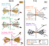 |
Fig. 1. Illustrations of the different geometries of the dust (left) and gas (right) models used in this work. The models are described in Section 2.1. In Tables 1 and 2, we describe the parameters of these models. The individual names used to refer to these models, from Section 3 onward, are shown in parentheses. |
2.2. Baseline model definition in the SFT: Mixing the X-ray and mid-IR models
In this work, we follow the simultaneous fitting technique proposed by Esparza-Arredondo et al. (2019). This technique combines X-ray and mid-IR models previously developed at each wavelength and their respective datasets. The SFT is performed through the XSPEC package, a command-driven interactive, spectral-fitting tool within the HEASOFT software2. XSPEC allows for one to fit data from different satellites such as ROSAT, Chandra, XMM-Newton, and NuSTAR with models constructed from single emission components coming from different mechanisms and physical regions. Most X-ray models are included in XSPEC, and it is possible to include new ones using the ATABLE task. We converted the mid-IR SED libraries of models to multi-parametric models within the spectral-fitting tool XSPEC as an additive table (see Section 4 of Esparza-Arredondo et al. 2019 and González-Martín et al. 2019b).
In this work, we define our baseline models as the following command sequence in XSPEC:
 (1)
(1)
where phabs is the foreground galactic absorption (see Col. 3 in Table 3), and zdust * zphabs * cabs represents the LOS absorption at the redshift of the source. The cutoffpl component is a power law with a high energy exponential rolloff that models the intrinsic component of X-ray emission. These X-ray absorbers are not evaluated at energies below 10−4 keV. However, the mid-IR and X-ray simultaneous fit requires the X-ray intrinsic emission to be properly absorbed below those energies. Therefore, we introduced a zdust component to neglect any artificial contribution of this component to mid-IR wavelengths and incorporated a foreground extinction at this range. The mid-IR and X-ray models are introduced through the command atable. We have the option to use either borus02 or UXClumpy torus model for the reflection component and reproduce the dust continuum with the Smooth, Clumpy, or Two-Phases torus model (see Section 2.1 for an individual description of models).
General information of the sample.
In our work Esparza-Arredondo et al. (2019), we have shown that combining the mid-IR and X-ray models in a single baseline model can bear significant advantages. One of them is the ability to link similar parameters. For instance, the inclination angle for the mid-IR models can be set to the same value as the X-ray model (i = θinc), thereby reducing the number of free parameters and simplifying the model.
3. Sample
The sample analyzed here contains 24 nearby AGNs (z < 0.4) drawn from our previous work by Esparza-Arredondo et al. (2021). In this preliminary work, we selected 36 sources from an initial sample of 169 AGNs with available archival Spitzer and NuSTAR data. These 36 AGNs have a non-negligible contribution to the reflection component at X-rays and are dominated by the AGN-heated dust at mid-IR. In Esparza-Arredondo et al. (2021), we individually fit the Spitzer and NuSTAR spectra of these sources with the Smooth or borus02 and Clumpy or UXClumpy torus models at mid-IR and X-ray.
Out of the 36 AGNs that we selected, we could not fit three of them (Mrk 1018, PG 1535+547, and ESO 428-G014) at X-ray wavelengths, and we could not fit four sources (Mrk 3, NGC 4388, ESO-097-G013, and MCG+07-41-03) at mid-IR with any of the four models that we tested. This means that the χ2/d.o.f. value was greater than 1.2. As a result, we excluded these seven objects from the analysis. We found that the Smooth (borus02) and Clumpy (UXClumpy) models cannot explain their mid-IR (X-ray) properties. Therefore, we reduced the sample size to 29 sources.
We next improved the analysis by fitting the 29 Spitzer spectra to the Clumpy Disk+Wind and Two-Phases torus models. This analysis shows four sources (RBS 0770, PG 1211+143, RBS 1125, and Mrk 1393) that require the Clumpy Disk+Wind model at mid-IR wavelengths. We also excluded them from this analysis because no simultaneous fit can be performed due to the lack of a self-consistent X-ray model for the disk+wind distribution. We also discarded MCG+01-57-016 because its X-ray spectrum is complex and could be associated with the accretion disk (Akylas et al. 2022). We shall study these 11 discarded AGNs in a forthcoming investigation using new and more complex models.
Therefore, the sample for this study comprises the remaining 24 nearby Seyfert galaxies, eight of which are type 1 (Sy1) and sixteen of which are type 2 (Sy2). Our sample covers three orders of magnitude in X-ray intrinsic luminosity (log(L2 − 10 keV)∼41.7 − 44.6), and three orders of magnitude in black hole mass (log(MBH)∼6.2 − 8.9). Table 3 (Cols. 1–7) shows the main observational details of the final sample.
4. Spectral fitting
We initially fit the Spitzer spectra of all sources using three different models: the Smooth, Clumpy, and Two-Phases torus models. To determine the best fit for the mid-IR data, we compared the resulting χ2 values of each source using the F-test statistic. Based on these results, Column 8 of Table 3 reports the preferred mid-IR model. Subsequently, we applied the SFT to all sources. In this step, we simultaneously charged the NuSTAR and Spitzer spectra of each source into XSPEC software and fit both spectra using a baseline model defined through the command sequence shown in Sect. 2.2 (see Eq. (1)). It is important to note that the baseline models are a combination of the best mid-IR model with one of the X-ray models (borus02 or UXClumpy). Hence, we have two simultaneous fits to each source at this stage, which combine the borus02 or UXClumpy with the best mid-IR model. In all our fittings, we assume that the viewing angle is the same for both mid-IR and X-ray models (θinc = i)3. Hereafter, we refer to the combination of the borus02 and UXClumpy torus models with either the Smooth, Clumpy, or Two-Phases torus models from mid-IR as the X-S/MIR-S, X-S/MIR-C, X-S/MIR-TP, X-C/MIR-S, X-C/MIR-C, and X-C/MIR-TP baseline models, respectively.
To choose the baseline model that best fits the Spitzer and NuSTAR spectra of each source, we ran the following analysis:
-
We linked the LOS column density (NHlos parameter) of the ZPHABS component to that of the reflection models (NHtor parameter). We considered all the fits with χ2/d.o.f. < 1.2 as a plausible solution for each source4. Subsequently, we used the minimum Akaike criteria to select the best baseline model, and all the fits with an Akaike probability below 0.1% were considered equally probable fits (as in Emmanoulopoulos et al. 2016).
-
When the borus02 torus model is part of the baseline model selected above, we also tested unlinking the NH parameters of the LOS from that of the reflection model5. We used F-test statistics to choose the simplest baseline model that describes the data.
-
After selecting the best baseline model, we tested the match of the half-opening angle (θtor) from the X-ray model to the value of the torus angular width (σtor) of the mid-IR model. The link between these parameters depends on the definition of the half-opening and torus angular width angles (θtor = σtor). In Fig. 2 (left), we compare the χ2/d.o.f obtained before and after linking these parameters. In Sect. 5.1, we provide a detailed analysis and comparison of the effect of linking and unlinking these parameters.
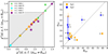
Fig. 2. Left: Comparison between χ2/d.o.f. values before and after linking the half-opening angle from X-ray models (θtor) and torus angular width from IR models (σtor), in all sources. The shaded area shows the χ2/d.o.f. values considered as a plausible solution. The baseline models are shown with different symbols and colors: X-S/MIR-C (green triangles), X-S/MIR-TP (pink pentagons), X-C/MIR-S (cyan circles), X-C/MIR-C (orange stars), and X-C/MIR-TP (purple squares). Right: Comparison between the half-opening angle from X-ray models and torus angular width (θtor vs σtor), using baseline models where the inclination angles are linked (θinc = i). Sy1 and Sy2 are shown as orange and blue symbols. The arrows show the upper and lower limits in θtor and σtor along the axes x and y, respectively.
As an extra test, we also ran some fits using a different baseline model for the mid-IR spectra, but they are always statistically worse than the ones obtained using the best fit at mid-IR. The results of these tests were compared using the Akaike criteria. Indeed, the model selection at mid-IR strongly relies on its spectral features (González-Martín et al. 2019b). This is not the case for the X-ray spectra, where we find that the best models obtained from the individual fit at X-rays might change from that obtained when the SFT is applied. This is because X-ray data alone cannot fully restrict the parameters of the models (Saha et al. 2022). Therefore, it is important to systematically test both borus02 and UXClumpy torus models for the simultaneous fit to ensure we use the best model combination for each object.
5. Results
In this section, we show the results obtained after applying the simultaneous fitting technique and apply the tests explained in the previous section. In Sections 5.1 and 5.2, we present the results obtained before and after linking the half-opening angle from the X-ray model to the same value of the torus angular width of the mid-IR model. We use statistical tests to compare the final statistics and the possible parameter constraints of both fits to each source in these two subsections. Meanwhile, in the Sect. 5.3, we show the values of several physical parameters such as the mass, covering factor, and outer radii of the torus derived from the parameters of the baseline models. In Section 5.4, we show the results obtained from comparing the torus properties of Sy1 and Sy2.
5.1. The best baseline model
Figure 2 (left panel) shows the χ2/d.o.f. values obtained before and after linking the half-opening angle of the X-ray model and the torus angular width of the IR models to the same value for each AGN. Most of the sources have good statistics when their NuSTAR and Spitzer spectra are fit with the best baseline model chosen (χ2/d.o.f. < 1.2). Only three sources (NGC 4507, NGC 1052, and J05081967+1721483) show relatively poor spectral-fitting statistics (1.2 < χ2/d.o.f. < 1.4) due to their mid-IR spectra, which are not well fit with the baseline model tested. We discard these three sources for the rest of the analysis and will study them in detail in future work. The spectral fits of these sources are shown in Figs. B.2–B.3 in Appendix B.
In Figure 2 (left panel), we also identify with different colors and symbols the five resulting combinations of X-ray and mid-IR models that best fit the spectra of sources: X-S/MIR-C (green triangles), X-S/MIR-TP (pink pentagons), X-C/MIR-S (cyan circle), X-C/MIR-C (orange stars), and X-C/MIR-TP (purple squares). Inside the shaded area, the X-C/MIR-C and X-C/MIR-TP baseline models are preferred for most sources: nine (two Sy1 and seven Sy2) and six (three Sy1 and three Sy2), respectively. The X-C/MIR-S baseline model is only preferred for one source: J10594361+6504063. NGC 7213 and NGC 1358 prefer the X-S/MIR-C baseline model. Meanwhile, the X-S/MIR-TP baseline model is preferred by three sources: IRAS 11119+3257, Mrk 231, and NGC6300. In Column 2 of Table 4, we reported the baseline model chosen for each source.
Simultaneous fit results (θtor ≠ σtor).
For the seven sources that prefer the borus02 torus model at X-ray, we can also explore the possibility that the column density parameters from the LOS and the reflection component differ. To test this hypothesis, we fit these sources with a baseline model where the column densities of the LOS absorption and X-ray model are different and independent (see Baloković et al. 2018). We then used an F-test to compare the χr2 values of these fits with the obtained values when the column densities of both components are the same. We found that only NGC 6300 prefers a baseline model where the column density of these two components is unlinked (that is NHtor ≠ NHlos).
Finally, we used the F-test to explore whether the half-opening angle from X-ray and torus angular width from mid-IR models could be linked at the same value as a possible indicator of the same structure producing both components. Indeed, among the 21 AGNs (8 Sy1 and 13 Sy2) with good statistics (χ2/d.o.f. < 1.2), only Mrk 590 preferred a baseline model without linking the half-opening angle and torus angular width (this object is slightly over the 1:1 diagonal line in the left panel of Fig. 2). As examples, the final fits of five sources, one for each resulting baseline model, are shown in Fig. 3. The residuals (ratio between data and model) are in the range of [–3 and 3], with the largest departures at mid-IR wavelengths at the 9.7 μm silicate features.
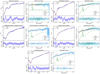 |
Fig. 3. Spectral fits of NGC 7213, NGC 6300, J10594361+6504063, ESO103-G35, and IC4518W. The solid orange lines are the best fit obtained from the X-S/MIR-C, X-S/MIR-TP, X-C/MIR-S, X-C/MIR-C, and X-C/MIR-TP baseline models. For each galaxy, the Spitzer spectrum is shown with blue points (left panel), and the NuSTAR spectra are displayed with blue and cyan points (right panels). The dashed magenta and green lines show the absorbed power law and the reprocessed components, respectively. The lower panels display the residuals between the data and the best-fit model. The data and residual errors are shown as shaded areas. |
To summarize, 95% of the sources in our sample favor a simple baseline model in which the half-opening angle and torus angular width parameters are linked to the same value. This result suggests that for most of our sources, the mid-IR continuum emission and the reflection component of X-ray stem from the same structure (Esparza-Arredondo et al. 2019).
5.2. Constraints on the model parameters
The SFT is an excellent tool to constrain most of the physical parameters of the obscuring material because it combines information from both X-ray and mid-IR wavelength ranges. To further explore this improvement, in each panel of Fig. 4, we compare the values of parameters before and after linking the half-opening angle and torus angle width. We use different symbols and colors to identify the baseline models chosen and the type of source, respectively. Additionally, in Tables 4 and 5, we report the final best model, χr2 obtained, and the parameters before and after linking the half opening angles, respectively. Quoted errors are estimated as one standard deviation.
Simultaneous fit results (σtor = θtor).
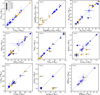 |
Fig. 4. Comparison between parameters before and after linking the half-opening angles (θtor) and torus angular width (σtor). Orange (blue) symbols are Sy1 (Sy2), and their shape denotes the best baseline model for each of them (see legend in panel 1). The lower and upper limit values are shown with black arrows. |
Concerning the X-ray parameters, we find that the Γ and NHtor parameters are constrained in most of the sources independently of whether the half-opening angle and torus angular width are linked or not, except by the column density of Mrk 1392 which is a lower limit when θtor = σtor. The viewing angle θinc parameter is constrained in six out of eight Sy1 and six out of the 13 Sy2 before and after linking the half-opening angle and torus angular width.
Among the mid-IR parameters, we find that, before linking the half-opening angle and torus angular width, the σtor parameter is constrained in 14 among the 20 sources with good statistics, and the parameter is unrestricted for only NGC 1358 (marked as asterisks in Col. 8 of Table 4). Interestingly, the unconstrained value for NGC 1358 results in an upper limit when we link the half-opening angle and torus angular width.
Before linking the half-opening angle and torus angular width, the parameter more difficult to constrain is θtor for most sources; it is only constrained to three Sy1 and one Sy2 (see Column 6 in Table 4). Indeed, in six sources, the half-opening angle could be any value (that is, not even upper limits are obtained). This is fixed by linking it to the mid-IR torus angular width (σtor). As was mentioned at the end of our previous subsection, this link is statistically preferred by most sources in our sample. However, it is worth exploring if the half-opening angle and torus angular width obtained prior to this link are consistent with it. In Fig. 2 (right), we compare the θtor and σtor values obtained when we only link the viewing angles (that is, both parameters are allowed to vary independently). The seven sources (NGC 4939, UM 146, Mrk 1210, NGC1358, J10594361+6504063, Mrk 231, and IC4518W) where one of the half-opening parameters is unrestricted are shown with gray marks. We find 12 where the σtor and θtor values are similar. Indeed, the values of both parameters are very different only for three sources (Mrk 1392, UM 146, and NGC 4939).
The size of the dusty torus is parameterized through the Y parameter, which is obtained from the mid-IR baseline models (X-ray models do not depend on the outer radius of the torus). This parameter is constrained in 11 out of the 20 AGNs, independent of whether the half-opening angle and torus angular width are linked or not. Finally, the slope of the radial density profile (αr) and optical depth (τν) are constrained in 15 and 11 sources, respectively. Regardless of whether the half-opening angle and torus angular width are linked or not (see panels 6–7 in Fig. 4).
As has been reported in our previous work, this technique of linking the half-opening angle and torus angular width is an excellent help to constrain the parameters further and break possible degeneration (Esparza-Arredondo et al. 2019). The analysis presented in this work confirms this result. To illustrate the improvement on the parameter restriction, Fig. 5 shows the two-dimensional χ2 distribution for each free parameter before and after linking the half-opening angle and torus angular width with dotted and solid lines, respectively, for ESO 138-G01. The black points and blue stars show the values reported in Tables 4 and 5, respectively6.
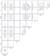 |
Fig. 5. Two-dimensional Δχ2 contours for the resulting free parameters when we used the X-C/MIR-C baseline model before (dotted lines) and after (solid lines) linking the half-opening angle and torus angular width to fit ESO 138-G01 spectra. The (dotted and solid) red, green, and blue contours mark the 1σ, 2σ, and 3σ errors, respectively. The black circles and blue stars are the resulting values for each parameter before and after linking the half-opening angle and torus angular width, respectively. These contours for the rest of the sources are available in this URL. |
For most of the sources, we find that parameters from the baseline models where σtor = θtor are better constrained at all levels. We can observe this result in the case of ESO 138-G01, where the viewing angles and torus angular width are much better restricted after assuming this link between parameters. The θtor parameter is the most difficult to constrain for most of the sources, even at the 1-σ level7. However, the σtor parameter is constrained in most of the sources at 2σ level, except for NGC 788, NGC 1358, Mrk 78, and PKS 2356-61. According to the f-test, Mrk 590 is the only source that prefers a baseline model without the half-opening angle and torus angular width linked (see previous subsection). We also find that the θinc and Y parameters are not constrained at any level for three (UM 146, NGC 1358, and Mrk 78) and two (IC 4518W, ESO 138-G1) sources, respectively. NGC 1358 is the source with fewer parameters constrained at the 2σ level (τ, Y, Γ, and NHtor are constrained). Furthermore, the θinc parameter of ESO 103-G35 could have two opposite values.
5.3. Dust quantities derived from mid-IR parameters
The outer radius of the torus (Rout), the total AGN dust mass (Mdust), and the covering factor (CF) are pivotal IR quantities that hold significant physical significance (Ramos Almeida & Ricci 2017, for a review). To obtain these important values, we derive them from the posterior distributions (PDs) of the parameters involved8. In Table 5, we report the final values for each of these quantities and their corresponding confidence interval. Determining the outer radius involves the Y parameter of each model and assumes the connection between the dust sublimation radius and AGN bolometric luminosity to derive the inner radius. Regardless of the baseline model chosen, the outer radius within our sample spans a range of values from 0.5 pc to 16 pc. Approximately 80% of our sample shows Rout < 5 pc. NGC 4507 has the highest Rout, while NGC 7213 hosts the smallest value. When considering a clumpy distribution of dust, the outer radius spans a broad range from 0.49 pc to 8.45 pc, except for NGC 4507. In contrast, the range narrows for sources favoring a two-phases distribution of the dust, ranging from 0.78 pc to 3.52 pc. The Rout for 2MASX J10594361+6504063 (the only one that prefers a Smooth torus model at mid-IR) agrees with the previously mentioned ranges.
To calculate the Mdust, we integrated the dust density distribution across the entire dust volume9. We used the definition of the density distribution given in the primary papers of the mid-IR models (see Fritz et al. 2006; Nenkova et al. 2008a; González-Martín et al. 2023). We find that the total dust masses of our sources range between log (Mdust) = [2.7 − 7.5]. NGC 4939 and 2MASX J10594361+6504063 show higher and lower dust mass values, respectively. The sources that prefer baseline models with a two-phases distribution of the dust have masses in the range log (Mdust) = [3.4 − 5.9]. Meanwhile, the sources that prefer baseline models with a clumpy distribution of the dust have extended masses between the range log(Mdust) = [2.5 − 6.5].
The Mdust and Rout values are consistent with those found in previous works (e.g., Lira et al. 2013; García-Bernete et al. 2019, 2022a). However, these measurements differ from those obtained using ALMA observations, which trace the cold dust and molecular gas distribution. For example, NGC 6300 and NGC 7213 are sources in common with the GATOS sample reported by García-Burillo et al. (2021). They measured outer radii and masses with higher values than in this work and in previous studies where mid-IR imagining and interferometric data were used (e.g., Packham et al. 2005; Radomski et al. 2008). The difference may be due to the mid-IR models not representing the observed physical size of dust by ALMA for the GATOS sample or the temperature differences that give rise to the emission of cold and hot gas (García-Bernete et al. 2022a). This result suggested that mid-IR only traces the inner parts of the torus where the dust has high temperatures and is mixed with gas traced through X-ray emission (see Lopez-Rodriguez et al. 2018; Alonso-Herrero et al. 2021; Nikutta et al. 2021b).
Finally, the calculation of the covering factor involves computing the unity minus the escape probability; that is, ∫e−τν(lso) Cos σtor dσtor, where τν(lso) is the LOS opacity. This opacity was computed from the equatorial opacity and the density distribution for Smooth torus models and from the distribution of clouds for Clumpy torus models. In the case of the Two-Phases torus model, the CF only depends on the sigma value. We find that CF values are in a broad range between [0.18–0.90]. Except for the CF of Mrk 1392, all Sy1s cover a range between [0.18:54]. Meanwhile, the Sy2s cover a range between [0.21:0.97]. A detailed analysis and discussion of these results is presented in Sect. 6.4.
5.4. Torus properties and AGN type
It is well established in the literature that the classical unification model is too simple to explain the properties and differences of Sy1s and Sy2s (see Ramos Almeida & Ricci 2017, for a review). Therefore, Sy2s are not only edge-on views of Sy1s, as the unification ideas propose (Urry & Padovani 1995). We find that most Sy1s (5 out of 8) have an inclination angle greater than 60°, suggesting an edge-on view system. However, the torus angular widths of these sources are small (< 20°). This indicates that their classification as type 1 sources is due to the torus not intercepting the LOS. Meanwhile, the θinc of Sy2s cover a wide range [21°:82°] (see panel 3 of Fig. 4). More than a decade ago already, pioneer works by Ramos Almeida et al. (2011) and Alonso-Herrero et al. (2011) using SED fitting at mid-IR wavelengths found intrinsic differences between Sy1 and Sy2 galaxies, besides the viewing angle. They found that the accretion disk of Sy1s is intrinsically less covered due to a thinner torus than that found in Sy2s. Using a volume-limited sample of nearby AGNs with sub-arcsecond angular resolution spectroscopy García-Bernete et al. (2019) confirmed these results.
Our results further confirm these differences. To illustrate it, Fig. 6 shows the PDs for each mid-IR parameter across our AGN sample, which includes both Sy1 and Sy2 populations. The histograms represent the combined PDs for all sources normalized by the area rather than individual PDs, providing a global view of the distribution of each parameter within the sample. The color coding highlights the differences between Sy1 and Sy2, facilitating a comparison of trends between the two types. The angular sizes, σtor, of Sy1 galaxies (orange) cover a narrow range between [10° −24° ] (except for the case of Mrk 1392). Meanwhile, the σtor values of Sy2 galaxies (blue) are grouped into two peaks; one is consistent with Sy1s while the other peak has a maximum at 60°. We confirm these results by comparing the PDs using the Kolmogorov-Smirnov (K-S) test10. The comparison between the Sy1 and Sy2 PDs shows that their distributions are different (p-value = 0.002). We also find clear differences in the covering factors. Except for Mrk 1392, all sources classified as Sy1s are consistent with CF < 0.5 and 11 out of the 13 Sy2s with good fits are consistent with CF > 0.5 (exceptions are IC 4518W and NGC 6300). The comparison of CF distributions of Sy1 and Sy2 through the K-S test confirms that the PDs are different (p-value = 0.04). The average covering factor of Compton-thin obscured AGNs analyzed by Zhao et al. (2021) at X-rays is CF ∼ 0.67, consistent with our results of Sy2 galaxies. García-Bernete et al. (2019) found that the CF obtained through only mid-IR fits depends on the torus dust distribution and geometry assumed by the model. They observed that using the Two-Phases torus models provides large values of covering factor (CF > 0.6), while the clumpy models tend to favor intermediate values. Although most baseline models chosen by our sources incorporate both mid-IR distributions inside the SFT, we did not observe this distinction in our sample. Instead, we found that the values of CF cover similar ranges, irrespective of the chosen baseline model.
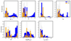 |
Fig. 6. Posterior distributions (PDs) of mid-IR torus model parameters for all AGNs in our sample with good statistics. The top row shows (from left to right) the torus angular width (σ = θtor), the ratio between the outer and inner torus (Y), the optical depth (τν), and the slope of the radial distribution of dust (αr). The bottom row shows the distribution of derived parameters (from left to right): covering factor (CF), total dust mass (Mdust), and the outer radius of the torus (rout). The orange and blue histograms correspond to Sy1 and Sy2, respectively. The white bars show the total combined distributions of Sy1 and Sy2. |
Recently, Kawamuro et al. (2024) used CIGALE code to model the full SED of the Sy1 Pox52, finding a torus with a small value of the angle between the equatorial plane and the edge of the torus (σtor), consistent with our results. No statistical differences are found regarding the total dust mass (p-value = 0.13 from K-S test) and, interestingly, among the five AGNs with Rout > 5 pc, four of them are classified as Sy2s, although AGNs with Rout < 5 pc are found for both Sy1 and Sy2 galaxies. The comparison of PDs of the Rout parameters of Sy1 and Sy2 reveals a p-value = 0.04, which implies that they are different distributions.
According to K-S test, with the exception of αr and Mdust, all parameter distributions differ between Sy1 and Sy2 (αr: p-value = 0.09, and Mdust: p-value = 0.13). Additionally, the PDs of Sy1 PDs differ from those of the total sample (p-value < 0.04), while the PDs of Sy2 are similar to those of the total sample (p-value > 0.27). Consequently, the mid-IR properties of the dust in Sy1s suggest that they belong to a well-defined group of objects with low covering factors and narrow half-opening angles, which increases the probability of the central photons escaping. In contrast, Sy2s are a mixed bag with highly covered objects, although the half-opening angle could be as low as that found for Sy1s.
X-ray parameters also reinforce this behavior when comparing Sy1s and Sy2s properties. To illustrate it, we show in Fig. 7 the column density of the reflection component, NHtor, versus the photon index, Γ, of the intrinsic continuum (associated with the X-ray corona). Most Sy1s show NHtor < 1022 − 23 cm−2 (20.6 < NHtor < 22.9) while Sy2s show larger values (23.0 < NHtor < 24.5). This is consistent with the X-rays classification of type-1/type-2 AGNs (Matt 2000). Zhao et al. (2021) investigated a sample of 93 obscured and nearby AGNs using only X-ray NuSTAR observations and the Smooth torus model. They found that Compton-thin and Compton-thick AGNs may harbor similar tori, whose average column density is nearly Compton thick (see also Buchner et al. 2019). This is consistent with our results for Sy2 galaxies. The photon index is also consistent with the canonical value of Γ = [1.8 − 2.1] for most Sy1s, while Sy2s show values as low as Γ = 1.5. Eleven out of the 13 Sy2 have Γ < 1.9 and all Sy1s have Γ > 1.9 (see panels 1 and 2 of Fig. 4). These two quantities anti-correlate with each other when we exclude the objects where an X-C/MIR-C baseline is preferred. Except for three sources (NGC 6300, ESO 138-G1, and UM 146), we observe that objects with a steeper X-ray intrinsic continuum are less obscured than those showing a flatter X-ray intrinsic continuum. This behavior is beyond the natural degeneration of the photon index and column density, which would imprint a positive correlation between these two quantities.
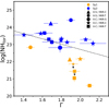 |
Fig. 7. Column density of the reflector (NHtor) versus the photon index (Γ). Sy1s are shown in orange, and Sy2s are shown in blue. Different symbols are shown according to the best models used for each object (see text). |
6. Discussion
6.1. Distribution of the dust and gas
One difference between the first SED fitting results (Ramos Almeida et al. 2009, 2011; Alonso-Herrero et al. 2011; Martínez-Paredes et al. 2017; García-Bernete et al. 2019) and those presented in this analysis is that they were based on a single SED library of models, consisting of a clumpy distribution of dust in a torus-like geometry. In the last few years, several studies have tested and compared models that propose new geometries and dust distributions available, including a disk+wind geometry (e.g., González-Martín et al. 2019a; Martínez-Paredes et al. 2021; García-Bernete et al. 2022a). These works found that the Clumpy Disk+Wind model is more suitable for reproducing the SEDs of type-1 and more luminous AGNs, whilst Clumpy torus models are preferred for less luminous and type-2 AGNs. However, recently González-Martín et al. (2023) found that the Two-Phases torus model can reproduce the 85–88% of the spectra of a sample of 68 nearby and luminous AGNs. As we mentioned in Sect. 3, we only found four Sy1 (RBS0770, PG1211+143, RBS 1125, and Mrk 1393) from a previous sample of 36 AGNs that fit better with the Clumpy Disk+Wind model at mid-IR wavelengths. We are not including the analyses of these sources in this work because of the lack of this geometry at X-ray wavelengths. However, we agree that fully understanding AGN obscuration requires looking beyond the geometry of the dust distribution.
Besides its geometry, the distribution of dust and gas, either clumpy or smooth, has also been discussed (Ramos Almeida & Ricci 2017). At mid-IR, the smooth distribution is not preferred for almost any Seyfert (García-Bernete et al. 2022a), but it is preferred for more extremely obscured objects (e.g., García-Bernete et al. 2022b; Efstathiou et al. 2022). This result is confirmed in our analysis where the smooth distribution is preferred at mid-IR only for the Sy2 IRAS J105943+65040 (see Table 5). The 52% and 43% of our sample require either a clumpy or a two-phases distribution of dust (11 and 9 AGNs, respectively). Most Sy1s prefer the two-phases distribution (5 out of 8 Sy1), while 8 out of the 13 Sy2s with good fits require the clumpy distribution of dust. Using full SED analysis and the CIGALE code to disentangle host and AGN contributions, Kawamuro et al. (2024) found that a Two-Phases torus better describes the emission for the Sy1 galaxy Pox 52 than a Smooth torus model, also consistent with our results.
At X-rays, the distribution of gas is still controversial, partially because of the lack of good datasets with enough information to distinguish between models (Saha et al. 2022). Despite that, recently, Sengupta et al. (2023) as part of the effort of the Clemson-INAF group (Marchesi et al. 2018; Zhao et al. 2021; Torres-Albà et al. 2021; Traina et al. 2021) to classify Compton-thick AGN candidates, found that 78% of the sources show a LOS column density different from that of the reflector, which they interpret as a preferred Clumpy distribution of the material. The Clumpy distribution of gas is preferred in 85% of the Sy2s analyzed here (only five AGNs prefer the borus02 torus model).
Now, if we consider gas and dust, we find a wide variety of distribution combinations that do not seem to be associated with the AGN type:
-
Clumpy distributions of both dust and gas (X-C/MIR-C baseline models): 2 Sy1s and 7 Sy2s.
-
Clumpy gas distribution and two-phases dust distribution (X-C/MIR-TP baseline model): 3 Sy1s and 3 Sy2s.
-
Smooth gas distribution and two-phases dust distribution (X-S/MIR-TP): 2 Sy1s and 1 Sy2.
-
Smooth gas distribution and clumpy dust distribution (X-S/MIR-C): 1 Sy1 and 1 Sy2.
These results highlight the complexity of the obscurer when considering multiwavelength information (Esparza-Arredondo et al. 2021).
Laha et al. (2020) investigated a sample of 20 Sy2s and found that 13/20 showed no significant variability in LOS column density, suggesting a smooth distant gas distribution. In our previous work, the smooth distributions of gas seemed to be preferred for AGNs without variable absorption, while the clumpy distribution of gas is needed when the object shows signs of LOS column density variability (Esparza-Arredondo et al. 2021). However, this was based on independent SED fitting of mid-IR and X-rays. Moreover, the Two-Phases torus model of the dust was not considered in our previous work. In the present work, where a baseline model is fit to both wavelengths simultaneously, this result is not confirmed. Laha et al. (2020) torus models incorporating both clouds or over-dense regions (two-phase distribution) should account for LOS column densities as low as a few 1021 cm−2. We speculate that including the Two-Phases torus model at mid-IR (without a counterpart at X-rays) in our current study might have weakened the link between column density variability and the chosen distribution of gas and dust. Perhaps new Two-Phases torus models at X-rays are needed, which could be done soon thanks to the extension of the radiative transfer code SKIRT that now accounts for the physics behind the X-ray reflection component (Vander Meulen et al. 2023).
6.2. Dust and gas connection
For decades, the relationship between gas and dust in different objects in the universe has been studied, and it is known that the properties of both materials are related (e.g., the metallicity or the grain growth Hensley & Draine 2023). In the case of the galaxies, this connection is supported by several scaling relations, for example, between the dust mass, total gas mass, stellar mass, and star-formation at different redshifts (e.g., Orellana et al. 2017; Popping et al. 2023). In this work, we explored the possible connection between the column density of the gas (NHtor) and the opacity τν of the dust. This relationship has been broadly studied in our Galaxy through different methods and considering the possible bias in the observations given rise to different quotient values between both variables (e.g., Reina & Tarenghi 1973; Gorenstein 1975). This work assumes the galactic dust-to-gas ratio presented by Draine (2003) and given as: NH/Av = 1.9 × 10²¹ [cm−2 mg−1] (Watson 2011). As is expected, for the sources that are further away from us, this relationship is affected due to the interstellar medium between the observer and the source (e.g., Kahre et al. 2018). In the case of AGN, Maiolino et al. (2001) find that this relationship is slightly above the Galactic dust-to-gas ratio.
Figure 8 compares the NHtor and τν values derived from the final best fits of each source. The dotted, solid, and dashed black lines show 10, 1, and 0.1 times the Galactic dust-to-gas ratio, respectively. Most Sy2 galaxies in our sample are consistent with the galactic values. Some of these galaxies show an increase in the NHtor value, which could be explained as due to dust-free neutral gas within the sublimation radius. Meanwhile, the Sy1 galaxies show slightly lower values for the galactic dust-to-gas ratio. These values agree with previous results (Burtscher et al. 2016; Huang et al. 2011). However, the low dust-to-gas ratio seen in Sy1s is hard to explain. Of course, variable absorption could be a reason. However, among the two Sy1s with restricted measurements of both NH and τV, Mrk 590 is not variable (Laha et al. 2020). Another possibility is that the gas within the sublimation radius has been expelled from the nucleus for these Sy1s throughout AGN winds and jets (see García-Burillo et al. 2021).
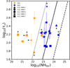 |
Fig. 8. Optical depth of the dust versus hydrogen column density of the gas. Sy1s are shown in orange and Sy2s are shown in blue. Symbols refer to the best baseline model per object. The dotted, solid, and dashed black lines show 10, 1, and 0.1 times the Galactic dust-to-gas ratio, respectively. Objects with upper/lower limits are shown with smaller symbols for clarity. |
6.3. Torus versus AGN luminosity
Intrinsic differences in the torus have also been claimed for high- versus low-luminosity AGNs (González-Martín et al. 2017). González-Martín et al. (2019a) found a larger percentage of best fits for the Clumpy Disk+Wind model for high-luminosity objects (see also Martínez-Paredes et al. 2021), while a larger number of low-luminosity AGNs were better fit to the Clumpy torus model (see also García-Bernete et al. 2022a). Furthermore, García-Bernete et al. (2022a) also showed that structural parameters, such as the outer radius of the torus, might depend on the luminosity of the source. To explore this, we delve into the possible relationships between the Lbol and the parameters characterizing dusty gas torus, as derived from our final fits. In Table 3, we report the bolometric luminosity, Eddington ratio, Lbol/LEdd, and the black hole mass, MBH, of each source.
We find a possible positive correlation between the total dust mass of the torus (log10(Mdust)) and the bolometric luminosity (log10(Lbol)), as depicted in Figure 9 (left panel). Considering all sources, this relation is not statistically robust, yielding a Pearson correlation coefficient11 (R) of 0.51 and a determination coefficient (R2) of 0.26. However, considering only the galaxies classified as Sy2, the correlation becomes more robust (R = 0.86 and R2 = 0.73). This result might show that the AGN luminosity is regulated by the amount of material available for AGN feeding or that the amount of AGN heated dust (and therefore emitting at mid-IR) is linked to the AGN luminosity. Although the accretion rates are affected by large uncertainties since no correlation is found between dust mass and the Eddington ratio (R = 0.17), the most natural explanation is that the total dust mass emitting in the mid-IR is directly linked to the AGN power heating the dust. Therefore, the current efficiency (λedd) of the accretion process would not be linked to the reservoir of material at parsec scales, which is expected considering the timescale for the torus to fall into the accretion disk (to nurture the AGN) is much longer than the timescales for the accretion disk to change its state. In the case of NGC 1068, the timescale estimate for the torus fade away is 1–4 Myr (García-Burillo et al. 2019). Meanwhile, the accretion disk is estimated to vary in timescales of hours (Hawkins 2007). Interestingly, although with larger dispersion (R = 0.40 and R2 = 0.15, see Figure 9 middle panel), a similar relationship is found for log10(Mdust) and log10MBH. This relationship suggests that a more massive SMBH can drag more dust from the circumnuclear medium into the AGN.
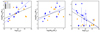 |
Fig. 9. First panel: Dependence of the torus total dust mass. Middle panel: Total dust mass versus the SMBH mass. Last panel: Slope of the radial distribution. Sy1s are shown in orange, and Sy2s are shown in blue. Symbols refer to the best baseline model found for each object (see legend in Fig. 2). The solid black and dashed blue lines show the best-fit linear relation between these two quantities considering all sources and only the Sy2, respectively. Objects with upper/lower limits are shown with smaller symbols for clarity. |
To study the robustness of the above relationship, we also explore if this dependence is due to the parameters involved in computing the total log10(Mdust), such as σtor, Y, αr, τν, and N0. No clear relationship is found between Lbol and neither τν, σtor nor N0 parameters. A robust link emerges between the bolometric luminosity and the slope of radial density distribution (R = −0.7 and R2 = 0.48, right panel of Fig. 9). For Sy2 galaxies, high αr values are associated with low log10(Lbol) values, indicating that the obscuring material is distributed closer to the nucleus in intermediate luminosity sources (αr > 1 and log10(Lbol) < 43.5 erg/s); meanwhile, the high luminosity sources tend to have a (relatively flat) distribution of material that extends further from the nucleus (αr < 1 and log10(Lbol) < 44 erg/s). Furthermore, most Sy1 tend to have lower αr values. It is important to notice that, even if limits are not considered in our statistical tests, four objects (NGC 4939, Mrk 590 and Mrk 1210, and Mrk 1392) are hard to reconcile within the general trend.
González-Martín et al. (2017) found evidence that the outer radius of the torus also decreases with the AGN bolometric luminosity for low-luminosity AGNs (log10Lbol < 42 erg/s). This behavior was confirmed for intermediate and high luminosity AGNs (41.7 < log10Lbol < 44.7 erg/s) by García-Bernete et al. (2022a). However, the latter authors do not find a clear dependence between Y and Lbol, suggesting that the correlation between torus size and Lbol might be caused, at least in part, by the sublimation radius, which is dependent on the Lbol. Our outer radii (Rout ∼ 1 − 9 pc) are in agreement with the range of mid-IR torus sizes estimated in previous works for nearby AGNs using data obtained through MIDI/VLT (e.g., Tristram et al. 2009; Burtscher et al. 2013). However, a clear linear dependence is not observed, partially due to the limited number of objects and the large amount of upper/lower limits in our results. It is important to remark that the SFT at both mid-IR and X-ray wavelengths does not help to restrict the outer radius of the torus because the X-ray reflection component does not depend on this parameter (most of the emission comes from the inner region of the torus Vander Meulen et al. 2023). Therefore, this parameter probably needs near-IR observations to be further constrained, as shown by Ramos Almeida et al. (2014).
6.4. Covering factor as a function of AGN accretion state
The covering factor is an effective parameter for understanding the role of the obscuring material in the context of the AGN feedback mechanism (Ramos Almeida & Ricci 2017, for a review). It is defined as the fraction of the sky obscured by the dust associated with the torus. There are different ways to measure this quantity, and several assumptions are present in all cases. Frequently, the CF is defined as the relationship between the nuclear-IR luminosity and the bolometric AGN luminosity (Maiolino et al. 2007; Treister et al. 2008; Gu 2013; Toba et al. 2021). This method assumes that the IR luminosity is dominated by the dust located within the torus and also assumes that both luminosities are isotropic (e.g., Stalevski et al. 2016; Rałowski et al. 2024). The CF can also be measured by counting the number of obscured sources at X-rays or the number of type-2 AGNs in volume-limited samples (Ueda et al. 2003; Ricci et al. 2023).
In this work, the CF parameter is derived from parameters obtained through mid-IR fit, so it is mostly associated with the dust-obscuring material (reported in Table 5, Col. 16). We find values between 0.15 to 1 (including error bars; see also the bottom-left panel in Fig. 6). The lack of values below CF < 0.15 is intrinsic to the modeling since all the models assume a torus angular size of at least σtor = 10° (see also González-Martín et al. 2019b). We carried out a general analysis of the derived CF in objects in common with the previous analysis, finding that the CF strongly depends on the method (and its assumptions). This is shown by González-Martín et al. (2019b), in which, even using the SED technique, the CF depends on the model assumed. Therefore, it is important to reinforce that these CFs are associated with dust, and that they assume a torus-like geometry.
In the last few decades, several works have revealed that there is an anticorrelation between the CF of AGNs and the accretion rate (Zhuang et al. 2018; Ezhikode et al. 2017; Toba et al. 2021) or the luminosity (Gu 2013). This relationship is interpreted by the fact that the inner radius of the obscuring material increases with the incident luminosity of the AGN (Ricci et al. 2017). Naddaf & Czerny (2024) find that the covering factor is intrinsically linked to the mass, accretion rate, and metallicity of the clouds under a scenario in which the clouds in the outer, less ionized part of the BLR are launched by the radiation pressure acting on dust. Ricci et al. (2023) compared the relationship between the Lbol and the covering factor obtained from the IR luminosity versus the CF from X-rays. They found a slightly less steep trend calculated through IR measurements compared with the trend found with the X-ray (see also Ananna et al. (2022)).
Figure 10 shows the covering factor values derived here versus the Eddington ratio. The solid and dashed gray lines show the trends, using X-ray data (dusty gas and dust-free) to derive CF, found by Ricci et al. (2022) for a sample of obscured AGNs. The area between the dashed gray lines represents the 1σ uncertainty around it. The solid and dash-dotted black lines show the trends that follow the median CFs obtained for obscured and unobscured sources from the sample of Ricci et al. (2023), derived through IR (dusty-gas) and using the correction of Vasudevan & Fabian (2007), respectively. All covering factors derived from our sample are inside the range of values that they reported. Objects with CF < 0.6 in our analysis seem consistent with the CF estimated from mid-IR by them. The CFs from X-ray are always above this trend (gray lines), indicating that the sources contain a significant contribution from gas. This is consistent with the work done by Ichikawa et al. (2019), where they found that the CF obtained from X-ray observations (gas) always exceeds the average CF of the dust.
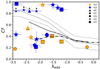 |
Fig. 10. Eddington ratio against covering factor (CF). The solid and dashed gray lines show the trend found by Ricci et al. (2022) and the 1σ uncertainty around it, respectively, when the covering factor of gas is inferred from the fraction of obscured sources using X-ray observations. The solid and dash-dotted black lines show the trends that follow the median CF, derived through IR data, obtained for obscured and unobscured, respectively, sources from the sample of Ricci et al. (2023). |
In an object-by-object comparison, except for Mrk 1392 and NGC 7213, all the sources classified as Sy1 of our sample appear to follow the trend found by Ricci et al. (2023) for unobscured sources (dash-dotted black line) together with four Sy2 (ESO138-G1, 2MASXJ10594361, NGC6300, and IC4518W). These four Sy2 sources show CFs and σ values that do not clearly distinguish them from Sy1s. However, the hydrogen column densities from X-rays are higher than those of Sy1. Therefore, the obscuration of these sources could be due to the distribution or density of the gas and dust. For example, NGC 6300 galaxy exhibit smooth and two-phase gas and dust distributions, respectively, which could explain their higher column density (log(NHtor) = 24.42) despite a relatively low dust mass (log(Mdust) = 3.45). In the case of the other three Sy2, their column density values are also higher and show low dust mass values, but their gas and dust distributions are in clumps and in two phases. A possible explanation is that gas clumps intercept the LOS but not dust clumps. These findings indicate that the obscuration mechanism in Sy2s is more complex. The remaining 60% of Sy2 shows higher CFs, and five are consistent with the trend obtained by X-rays. PKS 2356-61, ESO 103-G35, and Mrk 1210 are the sources with λedd > −1.5 and higher CFs that do not clearly follow the trend. Finally, IC 5063 is the only source with lower CF and λedd values.
Alternatively, the distribution of our sources in the λedd versus CF diagram may be related to past interactions between host galaxies and their neighbors. These interactions can create perturbations that influence both the black hole mass and the accretion rate (Krongold et al. 2002). For example, sources with higher CF ( > 0.5) and lower λedd, (< − 1.) can obscure the AGNs not only due to the dust and gas content or viewing angle but also due to the relatively low power of the AGN, which is insufficient to clear the surrounding material. Conversely, sources with lower λedd, (< − 1.) and CF ( < 0.5) may simply lack dust and gas. Meanwhile, objects like IRAS 11119+3257, which has higher λedd, (> − 1.) and lower CF ( < 0.6), could represent AGNs with sufficient energy to expel surrounding dust. In future work, we shall explore the environments of these galaxies to investigate this interpretation.
6.5. The column density as a function of AGN accretion state
The NH − λedd plane is used to explore the effect of the radiation pressure of the accretion disk on surrounding material (e.g., Venanzi et al. 2020; Alonso-Herrero et al. 2021; García-Bernete et al. 2022a; Vijarnwannaluk et al. 2024; Laloux et al. 2023, 2024). In Figure 11, we present the NHtor against the Eddington ratio for the sources of our sample. The solid black line shows “the effective Eddington limit”, introduced by Fabian et al. (2006). This limit considers the effect of the radiation pressure over the surrounding dust. It divides the plane into two regions known as the long-lived obscuration region and the forbidden region (or blowout region). The effective Eddington limit was reviewed considering the radiation-trapping and assuming different dust-to-gas ratios by Ishibashi et al. (2018). The radiation trapping could play an important role in the source where the obscuring material has a clumpy distribution; in this case, the reprocessed radiation tends to leak out through lower-density channels (that is, the path of least resistance), reducing the effective optical depth. The dashed cyan line in Fig. 11 shows the relationship assuming the galactic dust-to-gas ratio. Ishibashi et al. (2018) found that an increase in the dust-to-gas ratio implies that the forbidden region increases, meaning the dust is short-lived at lower Eddington ratios. Ricci et al. (2017) gave an evolutionary meaning to the NH − λEdd plane, where the AGN could move in this diagram during the life cycle. According to their recent work Ricci et al. (2023), there are four stages: (1) Accretion event, (2) Obscured phase, (3) Blowout phase, and (4) Unobscured phase. The radiation-regulated unification model agrees with the evolutionary sequence proposed by Krongold et al. (2002) and is discussed in our previous section.
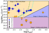 |
Fig. 11. NHtor–λEdd plane. The solid black line shows the effective Eddington limit introduced by Fabian et al. (2006). The dashed cyan and dash-dotted green lines show this limit if the radiation pressure on dust is considered, assuming one and two times the galactic dust-gas ratio, respectively. The shaded areas show the three areas that cover the different stages according to the radiation-regulated unification model proposed by Ricci et al. (2017). The solid gray line shows the limit where the NHtor could have an important contribution from the host galaxy. Symbols and colors follow the conventions used in the previous figures. |
The sources from our sample are located in the last three stages proposed by Ricci et al. (2023). IRAS11119+3257 is located in stage 3, where the CF and NHtor are consistent with a source where the accretion rate is so high that the obscuring material has been expelled. Tombesi et al. (2015) reported the detection of a powerful ultra-fast outflow in the X-ray spectrum of this source using Suzaku observations. They confirmed this result using NuSTAR observations and reported that the wind launching radius is likely at a distance of r ≤ 16 rs from the central black hole and has a mass outflow rate of ∼ 0.5 − 2 M⊙ yr−1 (Tombesi et al. 2017).
In the area defined for stage 2, we found that 76% of our sources and 62% are classified as Sy2, which is consistent with the prediction that obscured sources occupy this region with random inclination angles. Except for NGC 6300 and IC 4518W, all CFs are consistent with the mean value found by Ricci et al. (2023) for this stage. As mentioned in the previous section, these sources might have more circumnuclear material or an AGN with lower energy that is incapable of removing the material. Finally, the solid gray line marks the NHtor < 1022 limit, below which absorption by extended dust lanes may become important Fabian et al. (2008, 2009). According to Ricci et al. (2023), in this area, there are sources in stage 4, where most of the obscuring material has been expelled, and therefore, these sources would be observed as unobscured AGNs. ES0 141-G055, PG 0804+761, Mrk 1383, and Mrk 1392 are the four Sy1 galaxies located in this region. The three sources that chose the X-C/MIR-TP baseline model have CFs consistent with the mean value found by Ricci et al. (2023) for this region.
7. Summary and conclusions
In this work, we have used a simultaneous spectral fitting technique to study the properties of the dusty-gas torus in AGNs by analyzing NuSTAR and Spitzer spectra. Our sample consisted of 24 nearby AGNs (z < 0.4) selected from our previous study (Esparza-Arredondo et al. 2021): eight objects are type 1 Seyfert (Sy1), and sixteen are type 2 (Sy2). We utilized two and three X-rays and mid-IR models to fit the data, including the UXClumpy and Two-Phases torus models in our SFT, as an improvement over our previous work, enabling us to explore novel distributions of dust and gas.
Our technique allowed us to investigate whether the same structure could produce both X-ray reflection and mid-IR continuum. For this, we linked the half-opening angle and torus angular width values to the same value, as well as the inclination angles. This link between parameters implies fewer free parameters, and therefore simplifies the baseline models as it guarantees that the data are not over-fit. From a technical point of view, some of our main findings are that we are capable of successfully achieving good fits and constraining most physical parameters for most of the sample sources. Furthermore, the simplified baseline models also help to break the degeneracy among some parameters, such as, the column density and photon index.
While we acknowledge the need to enlarge the sample size for more robust results, our current findings strongly reinforce the evolution of the dusty gas around AGNs in several ways:
-
The mid-IR dusty torus in our sample shows inferred radii between 0.5 and 16 pc, and dust masses ranging from 102 to 107 M⊙.
-
We find a clear difference in the angular sizes of Sy1 and Sy2 galaxies. Most Sy1s have a torus angular width below ∼25°. This implies a covering factor below ∼0.5. On the other hand, Sy2s seem to be a mixed group with a broad distribution of torus angular width and covering factors. At X-ray wavelengths, the differences are even more evident; Sy1s show steep photon indices (Γ > 1.8) and low column densities for the torus (NH < 1022 cm−2), while Sy2s show large column densities (NH > 1022 cm−2) and a broader distribution of photon indices (1.4 < Γ < 2.2). Therefore, Sy1s and Sy2s have different dusty-gaseous structures.
-
Our analysis shows that their luminosity and mass influence the structure and distribution of the dusty gas torus in AGNs. A positive correlation exists between the total dust mass and bolometric luminosity for type 2 Seyfert galaxies (Sy2). This relationship suggests that AGNs with higher luminosities might have more available dust in their torus for feeding or that AGNs power heats the dust, leading to more mid-IR emission.
-
The clumpy−clumpy and clumpy−two-phases distribution is preferred for most sources (16 out of 23), although other combinations work better for some of the objects. It is important to note that the smooth distribution of dust is preferred only for one object in this analysis. Therefore, dust is distributed in clumps or in a two-phases medium, as suggested in previous works.
-
Our best fit is obtained when the column density of the reflection component is linked to that of the LOS; only NGC 6300 prefers them not to be linked. This suggests that the gaseous counterpart of the torus is homogeneous with a flat azimuthal distribution profile. Indeed, most of our models prefer a slope of azimuthal distribution in the mid-IR of αp < 0.5.
-
Our sources are located in three different states of the radiation-regulated unification model, with most currently in an obscuration phase. In the context of the evolution sequence of Seyfert galaxies, these sources may contain a more significant amount of circumnuclear material, or they may have an AGN with lower energy that cannot remove the material due to different factors. In future work, we shall analyze the environment of these sources to explore possible galaxy interactions, intrinsic properties, and environmental conditions.
It is important to remark that, among the parent sample of 36 AGNs studied by Esparza-Arredondo et al. (2021), three sources could not be fit with any model in the X-rays, and four sources could not be fit with any model at mid-IR. This indicates that further complexity from the models at both wavelengths is needed in a non-negligible fraction of AGNs. Additionally, four AGNs (all Sy1) prefer the Clumpy Disk+Wind model at mid-IR. Even though all of these sources were excluded due to the lack of a corresponding model in the X-ray, this indicates that the distribution of dust might vary for some objects. Models of X-rays with this distribution could help determine if the X-ray reflection is also produced by material associated with this clumpy disk+wind structure.
Data availability
The comparison of two-dimensional Δχ2 confidence contours for free parameters before and after assuming that the dust and gas emissions have the same origin structure for the sources of our sample are available in this Zenodo URL.
Note that the FeKα line and the Compton hump components might also be associated with reprocessing of the intrinsic emission at the accretion disk (Fabian 1998; Laor 1991).
Note that the viewing angle is measured with respect to the polar plane. A source observed face-on has an inclination angle of θinc = 19°, while a source observed edge-on has an inclination angle of θinc = 84°.
We chose the χ2/d.o.f. < 1.2 criterion to mitigate the underestimated errors of the Spitzer/IR spectra (See Appendix A in González-Martín et al. (2023)).
Only borus02 torus model allows one to untie the LOS NH from that of the reflection. UXClumpy torus model was computed assuming the same NH for both components.
Note that these values are located inside the 1sigma contour and do not necessarily have to be in its centers.
If the 3σ, 2σ, or 1σ contours cover a third of the total range of each parameter, then we consider that parameter is well constrained at the respective level.
We calculate the probability distribution function (pdf) for each quantity from the pdfs of the individual parameters involved. We use the STEPPAR command from XSPEC and divide the parameter space of each one into 30 equally spaced bins to obtain the individual PDFs.
We use the QUAD function within SCIPY (Python 3.0) to make all integration.
The null hypothesis is rejected if the p-value is lower than 0.05. Therefore, the PDs that we are comparing are different.
R2 = 1 means zero dispersion.
Acknowledgments
The authors thank the anonymous referee for the careful reading and constructive suggestions that improved the paper. D.E.A. is supported by the “Becas Estancia Postdoctorales por México” EPM(1) 2024 (CVU:592884) program of SECIHTI. D.E.A. acknowledges financial support from MICINN through the Juan de la Cierva program. O.G.M. and D.E.A. acknowledge financial support from PAPIIT UNAM IN109123 and “Ciencia de Frontera” CONAHCyT CF2023-G100. D.D. acknowledges financial support from PAPIIT,UNAM project IN111422. D.E.A. and C.R.A. acknowledge support from the Agencia Estatal de Investigación of the Ministerio de Ciencia, Innovación y Universidades (MCIU/AEI) under the grant “Tracking active galactic nuclei feedback from parsec to kiloparsec scales”, with reference PID2022-141105NB-I00 and the European Regional Development Fund (ERDF). D.E.A. and B.G.L. acknowledge support from the Spanish Ministry of Science and Innovation through the Spanish State Research Agency (AEI-MCINN/10.13039/501100011033) through grants “Participation of the Instituto de Astrofísica de Canarias in the development of HARMONI: D1 and Delta-D1 phases with references PID2019-107010GB100 and PID2022-140483NB-C21 and the Severo Ochoa Program 2020-2023 (CEX2019-000920-S). A.A.H. acknowledges financial support from the grant PID2021-124665NB-I00, funded by the Spanish Ministry of Science and Innovation and the State Agency of Research MCIN/AEI/10.13039/501100011033 PID2021-124665NB-I00, and by ERDFA’s Way of Making Europe. I.G.B. is supported by the Programa Atracción de Talento Investigador “César Nombela” via grant 2023-T1/TEC-29030 funded by the Community of Madrid. This work made use of data from the NuSTAR mission, a project led by CalTech, managed by JPL, and funded by NASA. We thank the NuSTAR Operations, Software and Calibration teams for support with the execution and analysis of these observations. This research has made use of the NuSTAR Data Analysis Software (NuSTARDAS) jointly developed by the ASI Science Data Center (ASDC, Italy) and CalTech. This work is based in part on observations made with the Spitzer Space Telescope, operated by the Jet Propulsion Laboratory, California Institute of Technology, under a contract with NASA.
References
- Aird, J., Coil, A. L., Georgakakis, A., et al. 2015, MNRAS, 451, 1892 [Google Scholar]
- Akylas, A., Papadakis, I., & Georgakakis, A. 2022, A&A, 666, A127 [NASA ADS] [CrossRef] [EDP Sciences] [Google Scholar]
- Alonso-Herrero, A., Ramos Almeida, C., Mason, R., et al. 2011, ApJ, 736, 82 [NASA ADS] [CrossRef] [Google Scholar]
- Alonso-Herrero, A., García-Burillo, S., Hönig, S. F., et al. 2021, A&A, 652, A99 [NASA ADS] [CrossRef] [EDP Sciences] [Google Scholar]
- Alonso-Herrero, A., García-Burillo, S., Pereira-Santaella, M., et al. 2023, A&A, 675, A88 [NASA ADS] [CrossRef] [EDP Sciences] [Google Scholar]
- Ananna, T. T., Urry, C. M., Ricci, C., et al. 2022, ApJ, 939, L13 [NASA ADS] [CrossRef] [Google Scholar]
- Antonucci, R. R. J., & Miller, J. S. 1985, ApJ, 297, 621 [NASA ADS] [CrossRef] [Google Scholar]
- Assef, R. J., Stern, D., Kochanek, C. S., et al. 2013, ApJ, 772, 26 [Google Scholar]
- Baloković, M., Brightman, M., Harrison, F. A., et al. 2018, ApJ, 854, 42 [Google Scholar]
- Buchner, J., & Bauer, F. E. 2017, MNRAS, 465, 4348 [Google Scholar]
- Buchner, J., Georgakakis, A., Nandra, K., et al. 2015, ApJ, 802, 89 [Google Scholar]
- Buchner, J., Brightman, M., Nandra, K., et al. 2019, A&A, 629, A16 [NASA ADS] [CrossRef] [EDP Sciences] [Google Scholar]
- Burtscher, L., Meisenheimer, K., Tristram, K. R. W., et al. 2013, A&A, 558, A149 [NASA ADS] [CrossRef] [EDP Sciences] [Google Scholar]
- Burtscher, L., Davies, R. I., Graciá-Carpio, J., et al. 2016, A&A, 586, A28 [NASA ADS] [CrossRef] [EDP Sciences] [Google Scholar]
- Combes, F., García-Burillo, S., Audibert, A., et al. 2019, A&A, 623, A79 [NASA ADS] [CrossRef] [EDP Sciences] [Google Scholar]
- Draine, B. T. 2003, ApJ, 598, 1017 [NASA ADS] [CrossRef] [Google Scholar]
- Efstathiou, A., Hough, J. H., & Young, S. 1995, MNRAS, 277, 1134 [Google Scholar]
- Efstathiou, A., Farrah, D., Afonso, J., et al. 2022, MNRAS, 512, 5183 [NASA ADS] [CrossRef] [Google Scholar]
- Emmanoulopoulos, D., Papadakis, I. E., Epitropakis, A., et al. 2016, MNRAS, 461, 1642 [NASA ADS] [CrossRef] [Google Scholar]
- Esparza-Arredondo, D., González-Martín, O., Dultzin, D., et al. 2019, ApJ, 886, 125 [Google Scholar]
- Esparza-Arredondo, D., Gonzalez-Martín, O., Dultzin, D., et al. 2021, A&A, 651, A91 [NASA ADS] [CrossRef] [EDP Sciences] [Google Scholar]
- Ezhikode, S. H., Gandhi, P., Done, C., et al. 2017, MNRAS, 472, 3492 [NASA ADS] [CrossRef] [Google Scholar]
- Fabian, A. C. 1998, AIP Conf. Ser., 431, 247 [Google Scholar]
- Fabian, A. C., Celotti, A., & Erlund, M. C. 2006, MNRAS, 373, L16 [NASA ADS] [Google Scholar]
- Fabian, A. C., Vasudevan, R. V., & Gandhi, P. 2008, MNRAS, 385, L43 [NASA ADS] [CrossRef] [Google Scholar]
- Fabian, A. C., Vasudevan, R. V., Mushotzky, R. F., et al. 2009, MNRAS, 394, L89 [NASA ADS] [CrossRef] [Google Scholar]
- Fritz, J., Franceschini, A., & Hatziminaoglou, E. 2006, MNRAS, 366, 767 [Google Scholar]
- Furui, S., Fukazawa, Y., Odaka, H., et al. 2016, ApJ, 818, 164 [NASA ADS] [CrossRef] [Google Scholar]
- Gámez Rosas, V., Isbell, J. W., Jaffe, W., et al. 2022, Nature, 602, 403 [CrossRef] [Google Scholar]
- García-Bernete, I., Ramos Almeida, C., Alonso-Herrero, A., et al. 2019, MNRAS, 486, 4917 [Google Scholar]
- García-Bernete, I., González-Martín, O., Ramos Almeida, C., et al. 2022a, A&A, 667, A140 [NASA ADS] [CrossRef] [EDP Sciences] [Google Scholar]
- García-Bernete, I., Rigopoulou, D., Aalto, S., et al. 2022b, A&A, 663, A46 [NASA ADS] [CrossRef] [EDP Sciences] [Google Scholar]
- García-Bernete, I., Alonso-Herrero, A., Rigopoulou, D., et al. 2024, A&A, 681, L7 [NASA ADS] [CrossRef] [EDP Sciences] [Google Scholar]
- García-Burillo, S., Combes, F., Ramos Almeida, C., et al. 2019, A&A, 632, A61 [Google Scholar]
- García-Burillo, S., Alonso-Herrero, A., Ramos Almeida, C., et al. 2021, A&A, 652, A98 [NASA ADS] [CrossRef] [Google Scholar]
- García-Burillo, S., Hicks, E. K. S., Alonso-Herrero, A., et al. 2024, A&A, 689, A347 [NASA ADS] [CrossRef] [EDP Sciences] [Google Scholar]
- González-Martín, O., Masegosa, J., Hernán-Caballero, A., et al. 2017, ApJ, 841, 37 [Google Scholar]
- González-Martín, O., Masegosa, J., García-Bernete, I., et al. 2019a, ApJ, 884, 10 [Google Scholar]
- González-Martín, O., Masegosa, J., García-Bernete, I., et al. 2019b, ApJ, 884, 10 [Google Scholar]
- González-Martín, O., Ramos Almeida, C., Fritz, J., et al. 2023, A&A, 676, A73 [NASA ADS] [CrossRef] [EDP Sciences] [Google Scholar]
- Gorenstein, P. 1975, ApJ, 198, 95 [Google Scholar]
- Gu, M. 2013, ApJ, 773, 176 [NASA ADS] [CrossRef] [Google Scholar]
- Hawkins, M. R. S. 2007, A&A, 462, 581 [NASA ADS] [CrossRef] [EDP Sciences] [Google Scholar]
- Hensley, B. S., & Draine, B. T. 2023, ApJ, 948, 55 [Google Scholar]
- Hönig, S. F., & Kishimoto, M. 2017, ApJ, 838, L20 [Google Scholar]
- Hönig, S. F., Kishimoto, M., Gandhi, P., et al. 2010, A&A, 515, A23 [CrossRef] [EDP Sciences] [Google Scholar]
- Hönig, S. F., Kishimoto, M., Tristram, K. R. W., et al. 2013, ApJ, 771, 87 [Google Scholar]
- Huang, X.-X., Wang, J.-X., Tan, Y., et al. 2011, ApJ, 734, L16 [Google Scholar]
- Ichikawa, K., Ricci, C., Ueda, Y., et al. 2019, ApJ, 870, 31 [NASA ADS] [CrossRef] [Google Scholar]
- Imanishi, M., Nakanishi, K., Izumi, T., et al. 2018, ApJ, 853, L25 [NASA ADS] [CrossRef] [Google Scholar]
- Imanishi, M., Nguyen, D. D., Wada, K., et al. 2020, ApJ, 902, 99 [CrossRef] [Google Scholar]
- Isbell, J. W., Meisenheimer, K., Pott, J.-U., et al. 2022, A&A, 663, A35 [NASA ADS] [CrossRef] [EDP Sciences] [Google Scholar]
- Ishibashi, W., Fabian, A. C., Ricci, C., et al. 2018, MNRAS, 479, 3335 [CrossRef] [Google Scholar]
- Kahre, L., Walterbos, R. A., Kim, H., et al. 2018, ApJ, 855, 133 [NASA ADS] [CrossRef] [Google Scholar]
- Kawamuro, T., Ricci, C., Yamada, S., et al. 2024, ApJ, 960, 15 [Google Scholar]
- Khim, H., & Yi, S. K. 2017, ApJ, 846, 155 [Google Scholar]
- Koss, M. J., Ricci, C., Trakhtenbrot, B., et al. 2022, ApJS, 261, 2 [NASA ADS] [CrossRef] [Google Scholar]
- Krongold, Y., Dultzin-Hacyan, D., & Marziani, P. 2002, ApJ, 572, 169 [Google Scholar]
- Laha, S., Markowitz, A. G., Krumpe, M., et al. 2020, ApJ, 897, 66 [Google Scholar]
- Laloux, B., Georgakakis, A., Andonie, C., et al. 2023, MNRAS, 518, 2546 [Google Scholar]
- Laloux, B., Georgakakis, A., Alexander, D. M., et al. 2024, MNRAS, 532, 3459 [NASA ADS] [CrossRef] [Google Scholar]
- Laor, A. 1991, ApJ, 376, 90 [Google Scholar]
- Leftley, J. H., Hönig, S. F., Asmus, D., et al. 2019, ApJ, 886, 55 [NASA ADS] [CrossRef] [Google Scholar]
- Lira, P., Videla, L., Wu, Y., et al. 2013, ApJ, 764, 159 [Google Scholar]
- Liu, Y., & Li, X. 2014, ApJ, 787, 52 [NASA ADS] [CrossRef] [Google Scholar]
- López-Gonzaga, N., & Jaffe, W. 2016, A&A, 591, A128 [NASA ADS] [CrossRef] [EDP Sciences] [Google Scholar]
- López-Gonzaga, N., Jaffe, W., Burtscher, L., et al. 2014, A&A, 565, A71 [NASA ADS] [CrossRef] [EDP Sciences] [Google Scholar]
- Lopez-Rodriguez, E., Fuller, L., Alonso-Herrero, A., et al. 2018, ApJ, 859, 99 [Google Scholar]
- Lopez-Rodriguez, E., Alonso-Herrero, A., García-Burillo, S., et al. 2020, ApJ, 893, 33 [NASA ADS] [CrossRef] [Google Scholar]
- Maiolino, R., Marconi, A., & Oliva, E. 2001, A&A, 365, 37 [NASA ADS] [CrossRef] [EDP Sciences] [Google Scholar]
- Maiolino, R., Shemmer, O., Imanishi, M., et al. 2007, A&A, 468, 979 [NASA ADS] [CrossRef] [EDP Sciences] [Google Scholar]
- Marchesi, S., Ajello, M., Marcotulli, L., et al. 2018, ApJ, 854, 49 [Google Scholar]
- Marconi, A., Risaliti, G., Gilli, R., et al. 2004, MNRAS, 351, 169 [Google Scholar]
- Martínez-Paredes, M., Aretxaga, I., Alonso-Herrero, A., et al. 2017, MNRAS, 468, 2 [Google Scholar]
- Martínez-Paredes, M., González-Martín, O., Esparza-Arredondo, D., et al. 2020, ApJ, 890, 152 [Google Scholar]
- Martínez-Paredes, M., González-Martín, O., HyeongHan, K., et al. 2021, ApJ, 922, 157 [CrossRef] [Google Scholar]
- Matt, G. 2000, A&A, 355, L31 [NASA ADS] [Google Scholar]
- Naddaf, M.-H., & Czerny, B. 2024, Universe, 10, 29 [Google Scholar]
- Nenkova, M., Ivezić, Ž., & Elitzur, M. 2002, ApJ, 570, L9 [NASA ADS] [CrossRef] [Google Scholar]
- Nenkova, M., Sirocky, M. M., Nikutta, R., et al. 2008a, ApJ, 685, 160 [Google Scholar]
- Nenkova, M., Sirocky, M. M., Ivezić, Ž., et al. 2008b, ApJ, 685, 147 [Google Scholar]
- Netzer, H. 2015, ARA&A, 53, 365 [Google Scholar]
- Nikutta, R., Lopez-Rodriguez, E., Ichikawa, K., et al. 2021a, ApJ, 919, 136 [NASA ADS] [CrossRef] [Google Scholar]
- Nikutta, R., Lopez-Rodriguez, E., Ichikawa, K., et al. 2021b, ApJ, 923, 127 [NASA ADS] [CrossRef] [Google Scholar]
- Ogawa, S., Ueda, Y., Tanimoto, A., et al. 2021, ApJ, 906, 84 [Google Scholar]
- Orellana, G., Nagar, N. M., Elbaz, D., et al. 2017, A&A, 602, A68 [NASA ADS] [CrossRef] [EDP Sciences] [Google Scholar]
- Osorio-Clavijo, N., González-Martín, O., Sánchez, S. F., et al. 2022, MNRAS, 510, 5102 [NASA ADS] [CrossRef] [Google Scholar]
- Packham, C., Radomski, J. T., Roche, P. F., et al. 2005, ApJ, 618, L17 [NASA ADS] [CrossRef] [Google Scholar]
- Pasetto, A., González-Martín, O., Esparza-Arredondo, D., et al. 2019, ApJ, 872, 69 [Google Scholar]
- Pier, E. A., & Krolik, J. H. 1992, ApJ, 401, 99 [Google Scholar]
- Popping, G., Shivaei, I., Sanders, R. L., et al. 2023, A&A, 670, A138 [NASA ADS] [CrossRef] [EDP Sciences] [Google Scholar]
- Radomski, J. T., Packham, C., Levenson, N. A., et al. 2008, ApJ, 681, 141 [NASA ADS] [CrossRef] [Google Scholar]
- Rałowski, M., Hryniewicz, K., Pollo, A., et al. 2024, A&A, 682, A120 [NASA ADS] [CrossRef] [EDP Sciences] [Google Scholar]
- Ramos Almeida, C., & Ricci, C. 2017, Nat. Astron., 1, 679 [Google Scholar]
- Ramos Almeida, C., Levenson, N. A., Rodríguez Espinosa, J. M., et al. 2009, ApJ, 702, 1127 [NASA ADS] [CrossRef] [Google Scholar]
- Ramos Almeida, C., Levenson, N. A., Alonso-Herrero, A., et al. 2011, ApJ, 731, 92 [Google Scholar]
- Ramos Almeida, C., Alonso-Herrero, A., Levenson, N. A., et al. 2014, MNRAS, 439, 3847 [Google Scholar]
- Reina, C., & Tarenghi, M. 1973, A&A, 26, 257 [NASA ADS] [Google Scholar]
- Ricci, C., Trakhtenbrot, B., Koss, M. J., et al. 2017, ApJS, 233, 17 [Google Scholar]
- Ricci, C., Ananna, T. T., Temple, M. J., et al. 2022, ApJ, 938, 67 [NASA ADS] [CrossRef] [Google Scholar]
- Ricci, C., Ichikawa, K., Stalevski, M., et al. 2023, ApJ, 959, 27 [NASA ADS] [CrossRef] [Google Scholar]
- Saha, T., Markowitz, A. G., & Buchner, J. 2022, MNRAS, 509, 5485 [Google Scholar]
- Sengupta, D., Marchesi, S., Vignali, C., et al. 2023, A&A, 676, A103 [NASA ADS] [CrossRef] [EDP Sciences] [Google Scholar]
- Siebenmorgen, R., Heymann, F., & Efstathiou, A. 2015, A&A, 583, A120 [NASA ADS] [CrossRef] [EDP Sciences] [Google Scholar]
- Stalevski, M., Ricci, C., Ueda, Y., et al. 2016, MNRAS, 458, 2288 [Google Scholar]
- Toba, Y., Ueda, Y., Gandhi, P., et al. 2021, ApJ, 912, 91 [NASA ADS] [CrossRef] [Google Scholar]
- Tombesi, F., Meléndez, M., Veilleux, S., et al. 2015, Nature, 519, 436 [NASA ADS] [CrossRef] [Google Scholar]
- Tombesi, F., Veilleux, S., Meléndez, M., et al. 2017, ApJ, 850, 151 [Google Scholar]
- Torres-Albà, N., Marchesi, S., Zhao, X., et al. 2021, ApJ, 922, 252 [CrossRef] [Google Scholar]
- Traina, A., Marchesi, S., Vignali, C., et al. 2021, ApJ, 922, 159 [NASA ADS] [CrossRef] [Google Scholar]
- Treister, E., Krolik, J. H., & Dullemond, C. 2008, ApJ, 679, 140 [Google Scholar]
- Tristram, K. R. W., Raban, D., Meisenheimer, K., et al. 2009, A&A, 502, 67 [NASA ADS] [CrossRef] [EDP Sciences] [Google Scholar]
- Tristram, K. R. W., Burtscher, L., Jaffe, W., et al. 2014, A&A, 563, A82 [CrossRef] [EDP Sciences] [Google Scholar]
- Ueda, Y., Akiyama, M., Ohta, K., et al. 2003, ApJ, 598, 886 [NASA ADS] [CrossRef] [Google Scholar]
- Urry, C. M., & Padovani, P. 1995, PASP, 107, 803 [NASA ADS] [CrossRef] [Google Scholar]
- van den Bosch, R. C. E. 2016, ApJ, 831, 134 [NASA ADS] [CrossRef] [Google Scholar]
- Vander Meulen, B., Camps, P., Stalevski, M., et al. 2023, A&A, 674, A123 [NASA ADS] [CrossRef] [EDP Sciences] [Google Scholar]
- Vasudevan, R. V., & Fabian, A. C. 2007, MNRAS, 381, 1235 [NASA ADS] [CrossRef] [Google Scholar]
- Venanzi, M., Hönig, S., & Williamson, D. 2020, ApJ, 900, 174 [Google Scholar]
- Victoria-Ceballos, C. I., González-Martín, O., Fritz, J., et al. 2022, ApJ, 926, 192 [NASA ADS] [CrossRef] [Google Scholar]
- Vijarnwannaluk, B., Akiyama, M., Schramm, M., et al. 2024, MNRAS, 529, 3610 [Google Scholar]
- Watson, D. 2011, A&A, 533, A16 [CrossRef] [EDP Sciences] [Google Scholar]
- Yang, G., Boquien, M., Buat, V., et al. 2020, MNRAS, 491, 740 [Google Scholar]
- Zhao, X., Marchesi, S., Ajello, M., et al. 2021, A&A, 650, A57 [NASA ADS] [CrossRef] [EDP Sciences] [Google Scholar]
- Zhuang, M.-Y., Ho, L. C., & Shangguan, J. 2018, ApJ, 862, 118 [NASA ADS] [CrossRef] [Google Scholar]
Appendix A: Equations to derive dust mass and covering factor parameters.
We integrate the density distribution of dust over the dust volume to obtain the Mdust. This density distribution depends on different parameters according to the baseline model. Using our notation for each parameter, the equations to compute the Mdust are as follows:
-
X-S/MIR-S, X-C/MIR-S, X-S/MIR-TP, and X-C/MIR-TP baseline models:
 (A.1)
(A.1) -
X-S/MIR-C and X-C/MIR-C baseline models
 (A.2)
(A.2)where C = 4.*π * mh * NH * τν * Rin2; NH = 1.9 × 10²¹; and mh = 1.76 × 10⁻²⁷.
We calculate the CF as the unity minus the escape probability; using our notation, the equations used are:
-
X-S/MIR-S, X-C/MIR-S, X-S/MIR-TP, and X-C/MIR-TP baseline models:
 (A.3)
(A.3) -
X-S/MIR-C and X-C/MIR-C baseline models
 (A.4)
(A.4)where C = 4.*π * mh * NH * τν * Rin2; NH = 1.9 × 10²¹; and mh = 1.76 × 10⁻²⁷.
In the case of the C-C and S-C baseline models, the Mdust is obtained using the N0, σtor, Y, and τν parameters. Meanwhile, the Mdust for the X-S/MIR-S, X-C/MIR-S, X-S/MIR-T, and X-C/MIR-T baseline models is derived through the αp, αq, Y0, and τν parameters.
Appendix B: Spectral fits
Final spectral fits of the sources of our sample. The solid orange lines are the best fit obtained from the X-S/MIR-C, X-S/MIR-TP, X-C/MIR-S, X-C/MIR-C, and X-C/MIR-TP baseline models. For each galaxy, the Spitzer spectrum is shown with blue points (left panel), and the NuSTAR spectra are displayed with blue and cyan points (right panels). The dashed magenta and green lines show the absorbed power law and the reprocessed components, respectively. The lower panels display the residuals between the data and the best-fit model. The data and residual errors are shown as shaded areas.
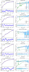 |
Fig. B.1. See the description at the beginning of this section. |
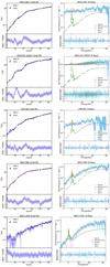 |
Fig. B.2. See the description at the beginning of this section. |
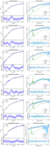 |
Fig. B.3. See the description at the beginning of this section. |
All Tables
Description and range of the parameters from the X-ray models used in this work.
All Figures
|
Fig. 1. Illustrations of the different geometries of the dust (left) and gas (right) models used in this work. The models are described in Section 2.1. In Tables 1 and 2, we describe the parameters of these models. The individual names used to refer to these models, from Section 3 onward, are shown in parentheses. |
| In the text | |
|
Fig. 2. Left: Comparison between χ2/d.o.f. values before and after linking the half-opening angle from X-ray models (θtor) and torus angular width from IR models (σtor), in all sources. The shaded area shows the χ2/d.o.f. values considered as a plausible solution. The baseline models are shown with different symbols and colors: X-S/MIR-C (green triangles), X-S/MIR-TP (pink pentagons), X-C/MIR-S (cyan circles), X-C/MIR-C (orange stars), and X-C/MIR-TP (purple squares). Right: Comparison between the half-opening angle from X-ray models and torus angular width (θtor vs σtor), using baseline models where the inclination angles are linked (θinc = i). Sy1 and Sy2 are shown as orange and blue symbols. The arrows show the upper and lower limits in θtor and σtor along the axes x and y, respectively. |
| In the text | |
|
Fig. 3. Spectral fits of NGC 7213, NGC 6300, J10594361+6504063, ESO103-G35, and IC4518W. The solid orange lines are the best fit obtained from the X-S/MIR-C, X-S/MIR-TP, X-C/MIR-S, X-C/MIR-C, and X-C/MIR-TP baseline models. For each galaxy, the Spitzer spectrum is shown with blue points (left panel), and the NuSTAR spectra are displayed with blue and cyan points (right panels). The dashed magenta and green lines show the absorbed power law and the reprocessed components, respectively. The lower panels display the residuals between the data and the best-fit model. The data and residual errors are shown as shaded areas. |
| In the text | |
|
Fig. 4. Comparison between parameters before and after linking the half-opening angles (θtor) and torus angular width (σtor). Orange (blue) symbols are Sy1 (Sy2), and their shape denotes the best baseline model for each of them (see legend in panel 1). The lower and upper limit values are shown with black arrows. |
| In the text | |
|
Fig. 5. Two-dimensional Δχ2 contours for the resulting free parameters when we used the X-C/MIR-C baseline model before (dotted lines) and after (solid lines) linking the half-opening angle and torus angular width to fit ESO 138-G01 spectra. The (dotted and solid) red, green, and blue contours mark the 1σ, 2σ, and 3σ errors, respectively. The black circles and blue stars are the resulting values for each parameter before and after linking the half-opening angle and torus angular width, respectively. These contours for the rest of the sources are available in this URL. |
| In the text | |
|
Fig. 6. Posterior distributions (PDs) of mid-IR torus model parameters for all AGNs in our sample with good statistics. The top row shows (from left to right) the torus angular width (σ = θtor), the ratio between the outer and inner torus (Y), the optical depth (τν), and the slope of the radial distribution of dust (αr). The bottom row shows the distribution of derived parameters (from left to right): covering factor (CF), total dust mass (Mdust), and the outer radius of the torus (rout). The orange and blue histograms correspond to Sy1 and Sy2, respectively. The white bars show the total combined distributions of Sy1 and Sy2. |
| In the text | |
|
Fig. 7. Column density of the reflector (NHtor) versus the photon index (Γ). Sy1s are shown in orange, and Sy2s are shown in blue. Different symbols are shown according to the best models used for each object (see text). |
| In the text | |
|
Fig. 8. Optical depth of the dust versus hydrogen column density of the gas. Sy1s are shown in orange and Sy2s are shown in blue. Symbols refer to the best baseline model per object. The dotted, solid, and dashed black lines show 10, 1, and 0.1 times the Galactic dust-to-gas ratio, respectively. Objects with upper/lower limits are shown with smaller symbols for clarity. |
| In the text | |
|
Fig. 9. First panel: Dependence of the torus total dust mass. Middle panel: Total dust mass versus the SMBH mass. Last panel: Slope of the radial distribution. Sy1s are shown in orange, and Sy2s are shown in blue. Symbols refer to the best baseline model found for each object (see legend in Fig. 2). The solid black and dashed blue lines show the best-fit linear relation between these two quantities considering all sources and only the Sy2, respectively. Objects with upper/lower limits are shown with smaller symbols for clarity. |
| In the text | |
|
Fig. 10. Eddington ratio against covering factor (CF). The solid and dashed gray lines show the trend found by Ricci et al. (2022) and the 1σ uncertainty around it, respectively, when the covering factor of gas is inferred from the fraction of obscured sources using X-ray observations. The solid and dash-dotted black lines show the trends that follow the median CF, derived through IR data, obtained for obscured and unobscured, respectively, sources from the sample of Ricci et al. (2023). |
| In the text | |
|
Fig. 11. NHtor–λEdd plane. The solid black line shows the effective Eddington limit introduced by Fabian et al. (2006). The dashed cyan and dash-dotted green lines show this limit if the radiation pressure on dust is considered, assuming one and two times the galactic dust-gas ratio, respectively. The shaded areas show the three areas that cover the different stages according to the radiation-regulated unification model proposed by Ricci et al. (2017). The solid gray line shows the limit where the NHtor could have an important contribution from the host galaxy. Symbols and colors follow the conventions used in the previous figures. |
| In the text | |
|
Fig. B.1. See the description at the beginning of this section. |
| In the text | |
|
Fig. B.2. See the description at the beginning of this section. |
| In the text | |
|
Fig. B.3. See the description at the beginning of this section. |
| In the text | |
Current usage metrics show cumulative count of Article Views (full-text article views including HTML views, PDF and ePub downloads, according to the available data) and Abstracts Views on Vision4Press platform.
Data correspond to usage on the plateform after 2015. The current usage metrics is available 48-96 hours after online publication and is updated daily on week days.
Initial download of the metrics may take a while.