| Issue |
A&A
Volume 698, June 2025
|
|
|---|---|---|
| Article Number | A16 | |
| Number of page(s) | 23 | |
| Section | Extragalactic astronomy | |
| DOI | https://doi.org/10.1051/0004-6361/202450685 | |
| Published online | 26 May 2025 | |
The Sunburst Arc with JWST
II. Observations of an Eta Carinae analog at z = 2.37
1
The Oskar Klein Centre, Department of Astronomy, Stockholm University, AlbaNova, 10691 Stockholm, Sweden
2
Institute of Theoretical Astrophysics, University of Oslo, P.O. Box 1029 Blindern, NO-0315 Oslo, Norway
3
Department of Astronomy, University of Michigan, 1085 S. University Ave, Ann Arbor, MI 48109, USA
4
Department of Physics, University of Cincinnati, Cincinnati, OH 45221, USA
5
Astrophysics Science Division, Code 660, NASA Goddard Space Flight Center, 8800 Greenbelt Rd., Greenbelt, MD 20771, USA
6
Department of Astronomy, University of Maryland, College Park, MD 20742, USA
7
Center for Research and Exploration in Space Science and Technology, NASA/GSFC, Greenbelt, MD 20771, USA
8
Department of Astronomy, University of Texas at Austin, 2515 Speedway, Austin, Texas 78712, USA
9
Department of Astronomy and Astrophysics, University of Chicago, 5640 South Ellis Avenue, Chicago, IL 60637, USA
10
Kavli Institute for Cosmological Physics, University of Chicago, Chicago, IL 60637, USA
11
Department of Physics and Astronomy and PITT PACC, University of Pittsburgh, Pittsburgh, PA 15260, USA
12
IPAC, California Institute of Technology, 1200 E. California Blvd., Pasadena, CA 91125, USA
⋆ Corresponding author: This email address is being protected from spambots. You need JavaScript enabled to view it.
Received:
10
May
2024
Accepted:
11
March
2025
Abstract
Context. The peculiar object known as Godzilla resides within the gravitationally lensed Sunburst Arc at z = 2.37. Despite being very bright, it appears in only one of the twelve lensed images of the source galaxy, exhibiting unusual spectroscopic properties that have not been found in any other clumps.
Aims. We use JWST’s unique combination of spatial resolution and spectroscopic sensitivity to propose a unified, coherent explanation of the physical nature of Godzilla.
Methods. We measured the fluxes and kinematic properties of rest-optical emission lines in Godzilla and its surrounding regions. Using standard line ratio-based diagnostic methods in combination with NIRCam imaging and ground based rest-UV spectra, we have characterized Godzilla and its surroundings.
Results. Among the set of around 60 detected lines, we found a cascade of strong O I lines pumped by intense Lyβ emission, as well as Lyα-pumped rest-optical Fe II lines, reminiscent of the Weigelt blobs in the local luminous blue variable (LBV) star Eta Carinae. The spectra and imagery of Godzilla and two faint adjacent images, along with the detection of a low-surface brightness foreground galaxy in the NIRCam data support the interpretation that Godzilla is an extremely magnified object, due to the alignment with lensing caustics. We find that Godzilla is part of a previously identified clump, comprising ∼10 − 25 % of it, with a magnification in the range of ≈600 − 25 000 (depending on the models and images used for comparison). The unique O I source in Godzilla is aptly explained as a non-erupting LBV accompanied by a hotter companion and/or gas condensations exposed to more intense radiation, compared to the Weigelt blobs. If Godzilla is confirmed to contain an LBV star in future studies, this finding would expand the distance to the furthest known LBV from a dozen Mpc to several Gpc.
Key words: circumstellar matter / stars: massive / galaxies: ISM / galaxies: individual: Sunburst Arc
© The Authors 2025
 Open Access article, published by EDP Sciences, under the terms of the Creative Commons Attribution License (https://creativecommons.org/licenses/by/4.0), which permits unrestricted use, distribution, and reproduction in any medium, provided the original work is properly cited.
This article is published in open access under the Subscribe to Open model. This email address is being protected from spambots. You need JavaScript enabled to view it. to support open access publication.
1. Introduction
Gravitational lensing magnifies distant objects. For a sufficiently small source (e.g., a single star), the magnification from a smooth galaxy cluster-scale lens can reach extreme levels (103 − 106, Miralda-Escude 1991). In realistic cluster-scale lenses, theoretical works have found that “microlenses”, namely, small-scale masses (e.g., stars) within the lensing cluster, perturb the lensing potential near the primary caustics and create a web of micro-caustics. These microcaustics cause the total magnification of the background lensed star to fluctuate. They also tend to limit the maximum magnification achievable (Venumadhav et al. 2017; Diego et al. 2018; Diego 2019).
The first lensed stars at cosmological distances (z ∼ 1 − 1.5) were discovered as transients in Hubble Space Telescope (HST) imaging, with magnifications that fluctuate as a result of microlensing (Kelly et al. 2018; Rodney et al. 2018; Kaurov et al. 2019; Chen et al. 2019). Since these initial discoveries, many more lensed stars have been found using this transient method (e.g., Kelly et al. 2022; Fudamoto et al. 2025). Additionally, several lensed stars have been identified from their proximity to the lensing critical curve (e.g., Meena et al. 2023; Diego et al. 2023a,b), including the most distant lensed star yet discovered at z ∼ 6 (Welch et al. 2022a,b).
Thus far, spectroscopic studies of lensed stars have proven difficult, owing to their transient nature or faintness. Furtak et al. (2024) present the James Webb Space Telescope (JWST) NIRSpec prism spectroscopy of a lensed star at z = 4.76, however they only detect stellar continuum, making it difficult to draw precise conclusions on the nature of the star.
In this paper, we study a lensed star candidate in the Sunburst Arc galaxy at z = 2.37. The Sunburst Arc is the brightest known strongly lensed galaxy at optical wavelengths, with an integrated magnitude mAB ≲ 18 (Dahle et al. 2016) and dozens of highly magnified and multiply imaged star-forming regions (Sharon et al. 2022). The Sunburst Arc earns its name from the strong “direct escape” Lyman-α (Lyα) emission (Rivera-Thorsen et al. 2017) and high fraction of Lyman Continuum (LyC) radiation escaping along the line of sight (LOS) from a single star-forming region (Rivera-Thorsen et al. 2019).
As a result of strong gravitational lensing, unresolved features in the Sunburst Arc (clumps or knots) are replicated multiple times along the arc. For example, the LyC-emitting clump (Sunburst LCE) shows an unusually extensive collection of 12 copied images. One unique clump as bright as Sunburst LCE, however, does not appear to have a counterpart anywhere else (Figure 1). Vanzella et al. (2020) found that this singly-imaged source in the northwest arc also exhibits highly unusual rest-ultraviolet (UV) features, such as Fe II emission lines excited by Lyα pumping (Bowen fluorescence, Bowen 1934), and has very high electron density ne ≳ 106 cm−3 probed by carbon and silicon emission doublets. Vanzella et al. (2020) first denoted this object as ‘Tr’, meaning transient. Diego et al. (2022) followed this notation and also dubbed the object ‘Godzilla’, whereas Sharon et al. (2022) referred to it as ‘a discrepant clump’. Recently, Pascale & Dai (2024) also adopted the name Godzilla, which is what we use here for the sake of a homogeneous terminology. For arcs and the IDs of the lensed images of clumps, we adopted the terminology of Sharon et al. (2022).
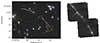 |
Fig. 1. Left: Overview of the north and northwest arc with the NIRSpec IFU pointings overlaid. The cyan, magenta, and yellow squares depict pointings 1, 2, and 3, respectively. We used NIRCam F115W, F200W, and F444W filters for R, G, and B, respectively. Godzilla in pointing 2 is marked with an orange arrow. (right) Pointings 2 and 3 showing Godzilla marked with an orange arrow. The images are oriented such that N is up, E is left. Each combined NIRSpec pointing is approximately |

Godzilla is believed to be an object residing in the Sunburst Arc galaxy, as its spectroscopic redshift is the same as the Sunburst Arc (z ≈ 2.37). The absence of any counterimages of Godzilla can be explained by an additional microlensing effect (Weisenbach et al. 2024) caused by a small object in front of Godzilla, extremely magnifying it only at that position (Diego et al. 2022; Sharon et al. 2022). Pascale & Dai (2024) has argued that Godzilla is a young, massive star cluster from spectral energy distribution (SED) fitting, but the absence of Godzilla counterimages is not clearly explained in that work.
An earlier explanation of Godzilla as a transient, akin to a supernova (SN, Vanzella et al. 2020) has since been ruled out by Diego et al. (2022) and Sharon et al. (2022). Furthermore, Diego et al. argued that Godzilla is likely to be a long-duration or stable source, rather than a typical SN. This assessment is based on that it has stayed bright for over five years in the observer’s frame (from 2016 to 2021). It surpasses typical SN durations of 1 to several months by far, although Vanzella et al. (2020) suggested at least one year of duration for an SN interacting with its circumstellar medium (CSM). Diego et al. also mentioned that archival imaging from 2014 (Dahle et al. 2016) shows Godzilla as a bright, unresolved source. Sharon et al. (2022) demonstrated that Godzilla did not clearly fade from February 2018 to December 2020 in HST imaging (Figure 9 therein). Depending on the observations considered, Godzilla was shown to maintain its luminosity for 1 (counted from 2018) to 1.93 (counted from 2014) years in the rest frame, correcting for cosmological time dilation. The SN scenario also contradicts the maximum time delay predicted from the lens model by Sharon et al. (2022). Relative time delays between the north arc and the northwest and west arcs are less than a year (Sharon et al. 2022, Figure 8). Thus, the counterimages of Godzilla would have been observed in other arcs if indeed Godzilla were a SN.
Previous studies on Godzilla gave special attention to η Carinae (η Car), a luminous blue variable (LBV) star in the Milky Way, as a possible analog. LBV is an umbrella term that includes previously defined Hubble-Sandage Variables, S Dor Variables, P Cyg, and η Car type stars as sub-types; it also specifically excludes Wolf-Rayet stars and blue supergiants (Conti 1984; Weis & Bomans 2020). LBVs are massive evolved stars (Weis & Bomans 2020, see their Figure 3), often surrounded by circumstellar nebulae as a consequence of their high mass-loss rate (Weis & Bomans 2020). These hot, unstable stars occupy an inclined instability strip of −11 ≤ Mbol ≤ −9 and 14 000 ≤ Teff ≤ 35 000 K in the Hertzsprung-Russell diagram (HRD) when they are quiescent; namely, not erupting (S Dor cycle, Wolf 1989). In some cases, they undergo ‘giant eruptions’, where the brightness increases by several magnitudes, as spectacularly observed for η Car in the year 1843 (known as the “great eruption”, as described in Humphreys et al. 1999) or in P Cygni in the 17th century (de Groot 1988). During the great eruption, η Car brightened to mV ≈ −1 (currently mV ≈ 4.01) and ejected at least 10 M⊙, thereby forming the Homunculus nebula (Davidson & Humphreys 2012, Ch. 7). Diego et al. (2022) demonstrated that the observed brightness of Godzilla can be achieved assuming a magnification factor of μ ≈ 7000 and an intrinsic brightness similar to that of η Car during the great eruption.
Vanzella et al. (2020) also pointed out that the Lyα-pumped Fe IIλ1914 detected in Godzilla has been observed in the Weigelt blobs in η Car (Johansson & Letokhov 2005). Weigelt & Ebersberger (1986) first discovered these three star-like gas condensations with diameters of < 0.03″(∼70 AU for a distance of 2300 pc) located within 0.1″– 0.2″from η Car using speckle interferometry. In 1995, HST resolved them in spectroscopy (Davidson & Humphreys 2012, Ch. 1.4) and revealed that they are slowly moving with a line-of-sight velocity of ∼40 km s−1, with densities of 107 − 108 cm−3 and temperatures of 6000–7000 K (Davidson & Humphreys 2012, Ch. 5). HST spectroscopy also revealed the 5.54-year spectroscopic cycle of η Car (Damineli 1996), where high excitation lines weaken when the hotter secondary star (40 − 50 M⊙, ∼4 × 10⁵ L⊙, Teff ≈ 39 000 K; Mehner et al. 2010) hiding behind the more massive, cooler primary star (≳90 M⊙, ∼106.7 L⊙, Teff ∼ 20 000 K; (Davidson & Humphreys 2012, 1.3.1)). Along with high excitation lines, Lyα-pumped and Lyβ-pumped lines such as Fe IIλ8453, Fe IIλ8490, and O Iλ8449 are strengthened when the Weigelt blobs are exposed to the hotter secondary star (Davidson & Humphreys 2012, see Figure 5.4).
The origin of the Weigelt blobs is the subject of ongoing research. It was previously believed that the Weigelt blobs were formed during a brightening in 1941 (Davidson & Humphreys 2012; Abraham et al. 2014). Abraham et al. (2020) used Atacama Large Millimeter Array (ALMA) observations to better constrain the proper motion (and, hence, the formation time) of the Weigelt blobs. They found that the three blobs are formed at different times (see their Fig. 16), but in each case, the blob formation coincides with epochs of minimum intensity in the high-ionisation lines in the spectrum of η Car. These epochs are also thought to coincide with the periastron of the hotter companion. There do not seem to be any particularly noticeable enhancements of the overall brightness of eta Car during these epochs (see e.g., the V-band and visual light curves in Fig. 3 of Fernández-Lajús et al. 2009).
Detecting extragalactic LBVs in spatially unresolved observations is highly challenging (e.g., Guseva et al. 2023). First, it is hard to capture the LBV phase of a star due to the short lifespan of this phase (Herrero et al. 2010, 104 − 105 years assuming single star evolution). Also, LBVs are not discernible from other bright hot stars during their quiescent phase, which can last for decades or centuries (Wofford et al. 2020). When they are not erupting, the S Dor variability is the only characteristic that distinguish LBVs from other massive, evolved stars (Weis & Bomans 2020). For these reasons, only a handful of LBVs have been observed and the farthest confirmed LBV is in DDO 68 which is 12.75 Mpc away (Makarov et al. 2017). If Godzilla is really an LBV, then this discovery extends the farthest known individual LBV star from one at a dozen Mpc to several Gpc (z = 2.37). However, many important traits of LBVs, such as broad hydrogen and often helium lines associated with P Cygni profiles (Guseva et al. 2023) as well as emission line nebulae and dust nebulae often surrounding LBVs, cannot feasibly be examined through ground-based telescopes at this redshift. Moreover, it was not possible to separate a pure spectrum of Godzilla uncontaminated by other features in previous ground-based slit spectroscopy. Thus, previous suggested explanations of Godzilla’s observed properties are based on the detection of a few exceptional emission lines or luminosity constraints from lens models. In this paper, we present JWST/NIRCam imaging and NIRSpec IFU observations of Godzilla for the first time. We have extracted the spatially resolved rest-optical to rest-near infrared (NIR) spectrum of Godzilla. Using imaging and spectroscopic data of unprecedented quality, we try to unveil the true nature of Godzilla.
The rest of this paper is structured as follows. In Section 2, we describe the observations and data reduction. In Section 3, we explain how we extracted spectra from Godzilla and four regions surrounding it. We also describe how we measured the kinematics and fluxes of emission lines, as well as the corrected measured flux for dust reddening. In Section 4, we describe main results, including the identification of almost 60 emission lines, the kinematics and gas properties of Godzilla, and the detection of Lyβ-pumped O Iλ8449 and Lyα-pumped iron lines (Section 4.4). In Section 5, we discuss various aspects of Godzilla. We first take a look at the NIRCam image and revisit SN and microlensing scenarios (Section 5.1). Then we identify counterimages including Godzilla and use them to derive the magnification of Godzilla (Section 5.2). To understand the O Iλ8449 source residing in Godzilla, we investigate spatial variations in the kinematics, dust, and gas properties by analyzing the surrounding regions (Section 5.3.1). We go through O Iλ8449 source candidates and exclude other scenarios (Section 5.3.2), showing that an LBV possibly with a hot companion analogous to η Car best explains the O Iλ8449 source (Section 5.3.3).
This paper assumes a flat ΛCDM cosmology with parameters ΩΛ = 0.7, Ωm = 0.3, and H0 = 70 km s−1 Mpc−1. With this cosmology, the redshift of the source, z = 2.37, corresponds to 2.72 Gyr after the Big Bang.
2. Observations
JWST observed the Sunburst Arc with NIRCam imaging and NIRSpec integral field spectroscopy (IFS) in the interval between 4-10 April 2023 (JWST Cycle 1, GO-2555, PI: Rivera-Thorsen). Imaging was done in each of the NIRCam filters F115W, F150W, F200W, F277W, F356W, and F444W. Two NIRSpec grating and filter combinations, G140H/F100LP and G235H/F170LP, were used to cover a rest-frame wavelength range of 0.29 μm ≤ λ0 ≤ 0.56 μm and 0.49 μm ≤ λ0 ≤ 0.94 μm, respectively. Of the three on-target NIRSpec pointings, Godzilla has been found in the pointing labeled 2 (i.e., the magenta square in Figure 1, indicated with an orange arrow). We refer to a companion paper by Rivera-Thorsen et al. (in prep.) for a full description of observations and data reduction.
We also used observed-frame optical (rest-UV), ground-based spectra collected with the Magellan Echellette (MagE) spectrograph on the Magellan-I Baade Telescope of the Las Campanas Observatory in Chile. This spectrum is the slit M3 pointing displayed in Figure 1 of Mainali et al. (2022) that covers Godzilla and two smaller, adjacent knots (the ‘P knots’, following the nomenclature of Diego et al. (2022)) seen in Figure 2. To summarize, we positioned the M3 slit on the arc by comparing the MagE slit viewing camera and HST images and we reduced the data as described in Rigby et al. (2018). For more in-depth descriptions of the MagE observations and the reduction process, we refer to Owens et al. (2024) for this pointing specifically. Furthermore, Rigby et al. (in prep.) will present a complete observation log for each pointing of the parent MagE observation program.
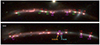 |
Fig. 2. Composite of NIRCam F115W, F200W, and F444W images of the north and the northwest arc of the Sunburst Arc. Images 3–10 of clump 4 are marked with purple circles, while images 1–10 of the LyC leaking clump (clump 1) are marked with red squares. In image 8 of clump 4 (4.8), we observe Godzilla and the P knots (the two small clumps). Images 1–4 of clump 5 are marked with green circles. These four images and image 4.7 (t1–t5 in Diego et al. (2022)) have been suggested as candidates for the counterimages of Godzilla by Diego et al. (2022). |
3. Methods
3.1. Extraction of 1D spectra
We extracted spectra from the brightest center of Godzilla (henceforth “the center”) and the four regions surrounding (NE, SE, NW, SW) to investigate the spatial variations of gas properties (Figure 3), along with the two P knots (named P1 and P2 for the left and right knot, respectively) for visual inspection. The spectra were extracted as a continuum-weighted spaxel average. The extracted spectrum of center appears in the top panel of Figure 4, with prominent lines labeled. The MAST instrument pipeline appears to underestimate errors, considering that the pipeline errors are smaller than the standard deviation of line-masked continuum regions in the spectrum itself. To correct this, we added the standard deviation of an empty region of sky in quadrature with the pipeline’s error estimate. We refer to Rivera-Thorsen et al. (in prep.) for a more in-depth explanation. In the bottom panel of Figure 4, we show the corrected uncertainties in the flux density for the G140H/F100LP and G235H/F170LP gratings in blue and red colors, respectively.
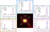 |
Fig. 3. Five regions where spectra have been extracted and their [O III]λλ4960,5008 doublet line profiles in the G140H/F100LP grating. The center figure shows the wavelength-axis median image of the NIRSpec G140H/F100LP grating at the area of Godzilla. Two-component (center, NW, SW) and one-component (NE, SE) Gaussian fits are also shown. |
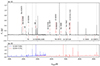 |
Fig. 4. Top: 1D spectrum extracted from the center region, labeled with prominent lines. Bottom: Corrected error from G140H/F100LP and G235H/F170LP gratings shown in blue and red, respectively. Noise pixels are marked with grey shades. Both flux density and errors from the two gratings are overlapped in ∼4925 − 5610 Å. See Figures B.1 and B.2 for more detailed features. |
Before measuring the fluxes, we subtracted the continua from the spectra. We first calculated the running-median and standard deviation (σ) of the spectrum with a rest-frame 100 Å wide moving window. After removing the data outside 3σ, we re-calculated the running median at the moving window and subtracted that result from the original spectrum.
3.2. Flux measurement
At the central, NW region, and SW region, we measured the flux of each line using two-component (narrow and broad) Gaussian fitting. Instrumental resolving power was accounted for by using the official NIRSpec calibration files2 and treating the linearly interpolated line spread function (LSF) as a Gaussian, which was adding to the model, along with the intrinsic linewidth in quadrature. We first measured the redshift and line width by fitting the strong oxygen doublet [O III]λ4960 and [O III]λ5008 simultaneously using a two-component Gaussian profile (Figure 3). Then we measured the flux of other lines in the same way (two-component Gaussian fitting), forcing each line to have the same redshift and velocity line width as the values measured for the [O III]λλ4960,5008 doublet at each grating. The error of the narrow, broad, and total fluxes were separately estimated using a Monte Carlo sampling method. The flux measured from the unperturbed spectrum was taken as the nominal value. For each wave bin, we then drew 999 random samples from a normal distribution, with (μ, σ) being the observed flux density and the uncertainty in that bin, respectively. Thus, we created 999 perturbed spectra. We repeated the fitting for the perturbed samples and reported the standard deviation of the 1000 measured fluxes as the error. We measured the flux in the NE and SE regions through the same procedure using only one Gaussian component, as additional components did not improve the fit here from visual inspection.
We found that the [O II]λλ3727,3729 doublet is distinctively red-shifted compared to other lines (Figure B.1). To accurately recover the flux and flux ratio of the [O II]λλ3727,3729 doublet, we allowed the redshift of these lines to vary, but kept the distance between the two lines fixed. At the center, the narrow component of [O II]λλ3727,3729 doublet is offset relative to [O III] (and to nearby higher-order Balmer lines) by the rest-frame 1.73 ± 0.6 Å (140 ± 50 km s−1). The broad component has a small offset consistent with 0 within the error bars.
In addition to a narrow and broad component, we found that a third, very broad component was necessary to obtain a good fit of Hα at the central, NE, and SE regions. We found no sign that this extra component was needed to obtain good fits for Hβ, [O III]λλ 4960,5008, or any other line. Figure 5 clearly shows the necessity of the very broad component in fitting Hα. The narrow and broad components of the [N II]λλ6550, 6585 doublet were set to have fixed ratios of 1:2.96 (Tachiev & Fischer 2001). In our spectra, there are a few more doublets arising from the same upper level, which have a fixed flux ratio (e.g., [O III]λλ4960,5008, [N III]λλ3870,3969, [O I]λλ 6302,6366), but we do not fix the flux ratio of these doublets. The two-Gaussian model is a simplification of the true line shape, and we found that additionally locking the line ratios led to over-constrained and over-simplified models producing poor fits. Allowing the line ratio to deviate slightly from the fixed value led to more accurate and better constrained models. The [N II]λλ6550,6585 doublet is the only exception from this, since [N II]λ6550 is completely buried in the very broad component of Hα and there is a chance of overestimating this broad component if we do not force the [N II]λ6550 flux to be ∼1/3 of the [N II]λ6585 flux. Figure 6 shows the fits of Hα and [N II]λλ6550,6585 with the third, very broad Hα component included. In the NW and SW regions, the fits of the very broad component of Hα had fluxes consistent with 0, so we did not include this third component for Hα in these regions.
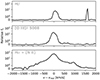 |
Fig. 5. Line profiles of Hβ, [O III]5008, and Hα+[N II] of the center region, highlighting the broad component present in Hα but not the other lines. The y-axis scale is linear between –1 and 1, and logarithmic outside this interval. The velocity scale in the lower panel is centered around Hα. |
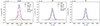 |
Fig. 6. Fitting result of Hα including a very broad component additional to default two component (center) and one component (NE, SE) Gaussian profiles. |
3.3. Dust reddening
We modeled the dust attenuation using a starburst attenuation law (Calzetti et al. 2000), assuming a standard RV = 4.05. We determined E(B − V) using Hα, Hβ, Hδ, H8, Pa9, and Pa10. We note that Hγ was not included since it partially lies on the detector gap, making its measured flux unreliable. We did not include H7 either, as this line is blended with [Ne III]λ3969. The itrinsic fluxes of Balmer and Paschen lines were calculated with PyNeb version 1.1.17 (Luridiana et al. 2015), assuming Te = 104 K and ne = 103 cm−3. The Balmer decrement can vary with density, but its effect is minimal. For example, at Te = 104 K, the Hα/Hβ ratio is 2.86 at a density of ne = 103 cm−3 and 2.81 at ne = 106 cm−3. When we take the simple average of the Hα/Hβ, Hδ/Hβ, H8/Hβ, Pa9/Hβ, and Pa10/Hβ ratios used in this study, the value changes only slightly from 0.65 at a density of ne = 103 cm−3 to 0.64 at ne = 106 cm−3. Therefore, to facilitate comparison with other studies, we adopted the value at a density of 103, which is commonly used as a standard value. We derived E(B − V) from each of the lines listed above and subsequently computed an error-weighted average (Figure 7). When averaging E(B − V), we excluded the very broad component of Hα for the central, NE, and SE regions. This is because including it consistently produced a higher value of E(B − V) from Hα than from the other lines. We note that there is a systematic uncertainty of ∼5.5 − 7.5% in the extinction-corrected flux that has not been included in the process of reddening correction. This uncertainty will affect all lines in a similar manner and therefore have a modest impact on derived line ratios.
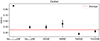 |
Fig. 7. E(B − V) as computed from the strongest Balmer and Paschen lines for the central region. The value from Hα is shown both including and excluding the very broad component. The average weighted by inverse of error is shown in red-dashed horizontal line with a shade representing 1σ uncertainty. Similar figures for the surrounding regions are shown in Figure C.1. |
4. Results
In this section, we focus mainly on kinematics and gas properties of the central region. When deriving gas properties, we used PyNeb version 1.1.17 for the electron temperature and density diagnostics.
4.1. Line identification
We detected 57 rest-optical emission lines (Tables A.1 and A.2), including auroral lines of four species (Figure 4). Contrary to previous observations that reported an absence of Balmer lines (Vanzella et al. 2020), we detected plentiful Balmer and Paschen lines with a signal-to-noise ratio (S/N) of up to ∼140. Interestingly, we detected a very strong permitted O Iλ8449. This line has been reported in Strom et al. (2023) from the stacked spectrum of z ∼ 1 − 3 galaxies, which they described as unexpected, since metal recombination lines usually are too weak and hardly detected even in local galaxies. Our detection is the first of its kind based on the spectrum of a single object at such a high redshift. We discuss this line in greater detail in Sections 4.4 and 5.4. In Tables A.1 and A.2, we list all the emission lines and their flux at the center, normalized by the total flux of Hβ. In this paper, we only use the total flux of each line, deferring a component-by-component analysis to future work.
4.2. Kinematics at the center
As described in Section 3.2, we computed the kinematic properties from the [O III]λλ4960,5008 lines, summarized in Table 1. We find a redshift for the narrow component of the [O III] doublet of zneb = 2.36983 ± 0.00003, averaged from the two gratings (see Table 1). This is slightly blue-shifted compared to the value of 2.37025 reported by Mainali et al. (2022), which has been measured from [O III]λ5008. However, Mainali et al. (2022) used ground-based spectra, integrating and averaging over a larger area of the sky. IFU velocity maps (Rivera-Thorsen et al. in prep.) show that Godzilla is blue-shifted relative to the systemic redshift.
Kinematics information for all regions. NE and SE regions only have narrow components, since we only performed a one-component Gaussian fitting for these regions.
In the G140H/F100LP grating, the narrow and broad component showed full width at half maximum (FWHM) of 37 ± 26 km s−1 and 216 ± 6 km s−1, respectively. In the G235H/F170LP grating, the FWHMs of the narrow and broad components were 110 ± 22 and 304 ± 35 km s−1. These are values corrected for the instrumental resolution. We suspect that the discrepancy in FWHM between the two gratings is the result of the poorer resolution of the G235H grating, and possibly from inaccuracies in the dispersion calibration files, which are all pre-flight. Although the FWHM is different in the two gratings, the measured fluxes of [O III]λλ4960,5008 are consistent within a few percent (Tables A.1, A.2). A very broad component observed in Hα is blue-shifted by 43 ± 14 and 83 ± 14 km s−1 relative to the narrow and the broad component at the rest-frame (z = 2.36929 ± 0.00015). It also has a large FWHM of 547 ± 31 km s−1. We found no evidence of an ongoing eruption. First, there is no clear P Cygni profiles in hydrogen and helium lines. Moreover, Hα at the center showed a maximum velocity of ∼1200 km s−1 (Figure 5) which is an order of magnitude smaller than the maximum velocity of Hα observed in η Car during the great eruption (∼104 km s−1, Smith et al. 2018).
4.3. Temperature and density diagnostics
We detected auroral lines from four species: [N II]λ5756, [O II]λλ7322,7332, [O III]λ4363, and [S III]λ6314. We note that the auroral line of [O III]λ 4363 is unusually high. As density diagnostics, we use [O II]λλ3727,3730 and [S II]λλ6718,6733, but the S/N of [S II]λλ6718,6733 is too low in some regions, including the center. As temperature diagnostics, we use [O II]λλ3727,3730/[O II]λλ7322,7732, [N II]λ5756/[N II]λλ6550,6585, [S III]λ6314/[S III]λ9071, and [O III]λ4363/[O III]λλ4960,5008.
At the center, PyNeb fails to find a convergent density and temperature solution using the observed diagnostics. Figure 8 clearly shows that density and temperature diagnostics are probing different gas phases. To explain the observed ratios of the auroral [O III]λ4363, [S III]λ6314, and [N II]λ5756 lines to their nebular counterparts, the gas should have density of ≳ 106 cm−3. The density range probed by [O II]λλ7322,7332 extends down to ∼104 − 105 cm−3, but still does not converge with the density solution from [O II]λλ3727,3730 of ≲103 cm−3. We emphasize that the narrow component of [O II]λλ3727,3730 is red-shifted by 140 ± 50 km s−1 in the rest-frame compared to the narrow component of [O III]λλ4960,5008. [O II]λλ3727,3730 might have an origin different from other emission lines, and may not be suitable as a density diagnostic. Previous observations found that the UV density diagnostic lines C III]λλ1907,1909 and Si III]λλ1883,1892 suggest a very high density of ne ≳ 106 cm−3 (Vanzella et al. 2020) in Godzilla. One of the main reasons for this discrepancy is that collisionally excited [O II] and [S II] start to be suppressed at relatively lower density (ncrit ≈ 4000 − 104 cm−3, Draine 2011) compared to other higher density tracers such as C III] (Kewley et al. 2019). We discuss this more in Section 5.3.1.
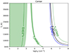 |
Fig. 8. Temperature and density solutions from PyNeb for the spectrum extracted from the center region in Figure 3. Oxygen, sulphur, and nitrogen diagnostics are depicted in green, grey, and blue colors, respectively, with shades representing the 1-σ confidence regions. We note that the Te [O II] diagnostic shown here might not be trustworthy, if indeed the [O II]λλ3727,3730 emission has a different region of origin than its auroral counterpart (see Section 3.2, Section 4.3). Similar figures for the surrounding regions are shown in Figure C.2. |
4.4. Bowen fluorescent lines
As reported in Section 4.1, we detect a strong O Iλ8449 line at the center, which has flux that is 20.75±0.15% of the Hβ flux, with S/N ≈ 139. We believe this line has mainly arisen from photo-excitation by accidental resonance (PAR) due to Lyβ photons, as suggested in Johansson & Letokhov (2005) and as reported for Lyα-pumped lines in Vanzella et al. (2020). The spectroscopic data disfavors other mechanisms, such as recombination, collisional excitation, or pumping by stellar continuum, considering very weak or absent O Iλ7776 and O Iλ7990, and the detection of rest-UV O I emission lines arising from PAR.
Figure 9 shows various O I lines in the rest-frame UV (a, b) and optical (c, d) wavelength. Panel c shows an absence of the O Iλ7776 triplet and O Iλ7990 complex. Measuring the ratio between O Iλ7776/λ8449 yields a 3σ upper limit of 0.009. This is inconsistent with the first two scenarios, since we expect λ7776/λ8449 ≈1.7 and λ7776/λ8449 ≈ 0.3 for the case of recombination and collisional excitation, respectively (Grandi 1980; Haisch et al. 1977). The line ratio O Iλ7990/λ8449 is expected to have a value of λ7990/λ8449 ≈ 0.052 from the continuum fluorescence cascade calculation by Grandi (1980) (assuming case B recombination and Te = 104 K). This is is inconsistent with the observed value 0.013 ± 0.005 in Godzilla, by more than 7σ, significantly weakening the stellar continuum excitation scenario. Assuming case A recombination, these ratios can become as low as 0.0030, but case A does not seem to be a proper assumption as we already know that there exists a dense gas component. O Iλ7256 is another line emitted from the same stellar continuum excitation cascade, but it falls in the detector gap.
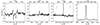 |
Fig. 9. a,b: Rest-frame UV spectrum of Godzilla from Magellan/MagE (Rigby et al. in prep.), showing the O I triplet and Si II line complex around 1304 Å and O I] 1641 Å. All these O I lines are part of the Lyβ pumped Bowen fluorescence cascade. c: NIRSpec spectrum showing position of the rest-frame optical O I recombination lines and/or stellar continuum excitation cascade triplet around 7776 Å and line complex at around 7990 Å, where we would expect to see line emission if the observed O I cascade were due to recombination or stellar continuum pumping. d: Lyβ-pumped, Bowen fluorescent O I 8449 Å. |
Moreover, we point out that the UV counterparts of Lyβ-pumped lines, the O I 1302.2, 1304.9, 1306.0 triplet and O I]λ1641.31 (Shore & Wahlgren 2010, see their Figure 1) emission lines, are detected in the MagE spectrum, although 1304.9 is not obvious due to the effect of Si II absorption (Figure 9-a, b). The observation of these other Lyβ-pumped lines of the same cascade, as well as the absence of recombination lines and continuum-pumped lines, supports that the permitted O Iλ8449 is a Lyβ-pumped line. Previously, emission near 1640 Å was identified as He IIλ1640.42 by Vanzella et al. (2020) and suggested as supporting evidence for a transient scenario. On the other hand, Diego et al. (2022) argued that it is O I]λ1641 based on its line center. Taking into account that we have detected other Lyβ-pumped O I lines while not detecting any He II emission lines, we conclude that this emission is from O I.
We also report the detection of Lyα-pumped Fe IIλ8490 with an S/N of 8. Interestingly, the other Lyα-pumped line near this line, Fe IIλ8453, has not been detected. Discussion of the Bowen fluorescent lines is continued in Section 5.4.
5. Discussion
5.1. Revisiting the transient scenario and the extreme magnification scenario
5.1.1. Transient scenario
The NIRCam data weakens the SN scenario suggested by Vanzella et al. (2020). Figure 2 shows the April 2023 NIRCam observation, and Godzilla still maintains similar brightness to that of the Sunburst LCE (clump 1, marked with red squares). It expands the observed duration of Godzilla from previously 2 years to 5 years. While Diego et al. (2022) included the original discovery ESO New Technology Telescope (NTT) observations in 2014 (Dahle et al. 2016), we exclude this as there Godzilla is not clearly resolved. Counting from the February 2018 HST observation, Godzilla has maintained its approximate luminosity for ∼1.5 years in the rest-frame.
Vanzella et al. (2020) argued that Godzilla (“Tr” in their terminology) is a Type IIn SN, a type of SN with narrow lines in their spectra. These narrow lines are believed to arise when a massive star explodes into a dense CSM. Although Type IIn SNe can be observed more than a few decades after explosion (Immler et al. 2005; Milisavljevic et al. 2012), it does not mean that it maintains a high luminosity for that extended length of time. One sub-type of Type IIn SNe, IIn-P (Mauerhan et al. 2013), is a type that shows a lasting, luminous plateau phase. A recent theoretical work however predicted the duration of this plateau phase to around 100 days at most (Khatami & Kasen 2024). Thus, a luminous plateau lasting for at least 1.5 years observed in Godzilla is highly unlikely to happen in any kind of SN known so far.
Godzilla is also unlikely to be some other kind of rare transient that shows an approximately flat light curve for 1.5 years. As summarized in Section 1, such a scenario contradicts the maximum time delay predicted from the lens model by Sharon et al. (2022), as a sudden increase in luminosity should have been observed in counter images in other arcs.
5.1.2. Extreme magnification scenario
Godzilla and a pair of clumps next to it (the ‘P knots’, following Diego et al. 2022) are believed to be nearby in the source plane (Diego et al. 2022). An extreme magnification can happen if Godzilla lies on the critical curve, as suggested in Diego et al. (2022). In Figure 10, we compared emission line profiles normalized by the flux of [O III]λ5008 at each spectrum for the P knots, Godzilla, and the Sunburst LCE. The left and right clumps in the P knots, P1 and P2, show nearly identical line profile traits such as redshift, line ratios and line width in various emission lines, and are clearly distinguished from Godzilla. It suggests that the P knots are likely to be the mirrored image of the same object different from Godzilla, and strengthens the hypothesis of a perturbing mass in the foreground generating a critical curve crossing the top of Godzilla and between the P knots (Diego et al. 2022, see Figure 6).
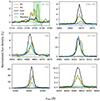 |
Fig. 10. Selected relative line fluxes from Godzilla, the two P-knots, and for comparison the Lyman Continuum emitter (LCE) knot, highlighting kinematics and relative line strengths. The green shaded interval in the [O II] panel indicates where P2 suffers from contamination from noisy pixels. The spectra were first normalized by their median value, the continuum then subtracted, and the resulting lines all normalized by the integral of [O III] 5008 of each spectrum. |
The plausibility of this lensing scenario is strengthened by the NIRCam detection of a low surface brightness galaxy centered only 0.5″from Godzilla. As shown in Figure 11, this galaxy has a clumpy structure and may be responsible for creating the small-scale perturbations needed to shift the critical curve to the locations suggested by Diego et al. (2022).
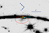 |
Fig. 11. Combined NIRCam F115W+F150W image, smoothed by a FWHM = 0.1″Gaussian to bring out low surface brightness details. The dashed ellipsoid marks a low surface brightness galaxy close to Godzilla (larger circle) and the P knots (smaller circles). |
5.2. Magnification factor derived from counterimages
5.2.1. Counterimages of Godzilla
Diego et al. (2022) suggested images 5.1–5.4 (marked with green circles in Figure 2) and 4.7 as candidate counterimages of Godzilla based on that they are located between images of clumps 1 and 2. On the other hand, the lens model from Sharon et al. (2022) predicts that Godzilla and the P knots together make up the highly resolved 8th counterimage of Clump 4 (depicted with purple circle labeled ‘4.8’ in Figure 2).
To identify possible counterimages of Godzilla, which should have a similar SED as Godzilla, we examined the SEDs for Godzilla, the P knots, and the images of clumps 1, 4, and 5. Using Photutils (Bradley et al. 2024), we extracted flux from 0.06 arcsec radius circular apertures, using the images taken with 6 NIRCam filters (F115W, F150W, F200W, F277W, F356W, and F444W). A color-color diagram was then created by combining the filters that displayed the most distinct differences in SED shape (F200W–F277W versus F277W–F356W), as shown in Figure 12. The stellar continuum properties of Godzilla appear to be closer to clump 4 than to clump 5. The P knots also occupy a position on the color-color diagram that is indistinguishable from clump 4.
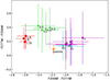 |
Fig. 12. Color-color diagram using the NIRCam F200W, F277W, and F356W filters. Error bars are shown for each point. In the color-color space, Godzilla (orange pentagon) is positioned closer to the images of clump 4 (purple circles, ‘4.’ in ‘4.X’ has been omitted) and P knots (cyan triangles). Its location is clearly distinguished from that of the images of clump 1 (red squares) and clump 5 (green thin diamonds). |
The unusually bright O Iλ8449 in Godzilla provides an additional method for investigating its counterimages. Figure 13 shows the O Iλ8449/[O III]λ5008 map for the north arc and northwest arc, revealing that strong O Iλ8449 emission is a unique feature of only Godzilla, P knots and clump 4, aside from the bright areas corresponding to image 8.4 in the pointing 1. Of the clump 5 images, only image 5.4, located next to image 1.4, falls within the NIRSpec pointing area and does not show strong O Iλ8449. To test whether this is due to suppressed [O III]λ5008 caused by high density, we have normalized O Iλ8449 with Hβ (Figure D.1). We observe an O I excess in the same regions as seen in the [O III]λ5008 normalization map, and image 5.4 still shows no elevation. Thus, the elevation in O Iλ8449 is not the result of suppressed [O III]λ5008 in the high-density region. We believe that the [O III]λ5008 emission observed in the Godzilla region originates from high-density gas with ne ≳ 106 cm−3. As shown in Figure 8, [O III]λ5008 probes regions with ne ≳ 106 cm−3, regardless of temperature. While the O I/Hβ ratio is also influenced by oxygen abundance, the O Iλ8449/[O III]λ5008 map, which is independent of metallicity, shows that the elevated O Iλ8449 is not due to high oxygen abundance. O Iλ8449 exhibits an elevation due to a unique Lyβ-pumping mechanism, which helps constrain the counterimage of Godzilla. Through a photometric colour comparison (Figure 12) and the O Iλ8449 maps (Figures 13, D.1), we concluded that images of clump 4 and P knots are counterimages containing Godzilla, as they share a similar stellar continuum color and characteristic nebular emission.
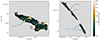 |
Fig. 13. O Iλ8449/[O III]λ5008 map for Pointing 1 (left) and Pointings 2+3 (right), with the stellar continuum overlaid as contours. The O Iλ8449/[O III]λ5008 ratio is near zero in the images of clump 1 and is highest in the images of clump 4, Godzilla, and the P knots. Refer to Figure D.1 in the appendix to see the map normalized by Hβ. |
5.2.2. Discrepancy between the stellar continuum and O I flux ratios in counterimages
The magnification factor of the candidate counterimages is known from the gravitational lens model; therefore, by comparing the flux of the candidate counterimages with that of Godzilla, we can determine Godzilla’s magnification factor. However, simply comparing the stellar continuum brightness is not sufficient. Sharon et al. (2022) considers Godzilla and the P knots as an enlarged version of clump 4, which makes direct flux comparison difficult if Godzilla is indeed a part of clump 4. Since O Iλ8449 is a very unique line, if we assume that the only source of O Iλ8449 observed in clump 4 is inside Godzilla and that there are no other major O Iλ8449 sources, comparing the brightness of O Iλ8449 between the clump 4 images and Godzilla would provide a more accurate comparison.
We extracted one-dimensional (1D) spectra from Godzilla, the two P knots (P1, P2), and images 4.4 and 4.9. We did not include image 4.10, as its close proximity to the bright image 1.10 might cause contamination. To measure the total O Iλ8449 flux for Godzilla, we re-extracted its spectrum over a 7 × 5 pixel area that includes the five regions (center, NE, SE, NW, SW) shown in Figure 3. The continua have been removed following the method described in Section 3.1, then we summed the flux of the O Iλ8449 line within the extraction area. We also compared the flux of the stellar continuum using photometry measurement employed for SED and color comparison in the previous section. The results are shown in Table 2.
Flux ratio compared to candidate counterimages and the derived magnification factor.
Godzilla exhibits a large discrepancy between its continuum flux ratio and its O Iλ8449 flux ratio. Compared to image 4.4, Godzilla’s continuum flux is 7.6 times brighter, while its O Iλ8449 flux is much brighter than that of image 4.4 with the ratio of 35. Assuming that Godzilla is the sole O Iλ8449 source, a flux ratio of 35 would be a more likely measure of the true magnification ratio between the two images. Under the assumption of a homogeneous magnification across the Godzilla region, the fact that the stellar continuum is only 7.6 times brighter suggests that the Godzilla region contains ∼22% (7.6/35 × 100) of the stars compared to image 4.4. Meanwhile, P1 and P2 do not show significant differences between their continuum flux ratios and O Iλ8449 flux ratios when they were compared to image 4.4. From this, we can infer that P1 and P2 represent the entirety of image 4.4, rather than just a part of it. The magnification factor for image 4.4 has derived to be  from Pignataro et al. (2021) and
  from Sharon et al. (2022). Combining these magnification factors with the O I flux ratio, the magnification factors for Godzilla, P1, and P2 are inferred to be μ ≈ 560, μ ≈ 20, and μ ≈ 25, respectively.
Comparing to image 4.9 presents a slightly different picture. The difference between the stellar continuum and O Iλ8449 flux in Godzilla is even more pronounced in this comparison, where the continuum flux ratio is ∼9.5 and the O Iλ8449 flux ratio soars to ∼94. Interpreting this with the same logic as before suggests that Godzilla contains only ∼10% of the stars present in clump 4. In the meanwhile, P1 and P2 show discrepancy of only factor of 2. The magnification factors for image 4.9 vary significantly between the two models presented. Pignataro et al. (2021) reported the magnification factor for image 4.9 to be  while Sharon et al. (2022) reported it as
  , noting the magnifications of images 1.9, 1.10, 4.9, and 4.10 should not be taken at face value. The magnification factors for Godzilla are then inferred to be μ ≈ 6700 and μ ≈ 2900 based on the models from Pignataro et al. (2021) and Sharon et al. (2022). This is all summarized in Figure 14, which clearly displays the variations in Godzilla’s magnification factor and the percentage of stellar components based on different images and models.
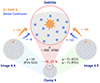 |
Fig. 14. Illustration explaining the relationships between clump 4, its two counterimages (images 4.4 and 4.9), and Godzilla. The difference between the O Iλ8449 flux ratio and the stellar continuum flux ratio indicates that Godzilla contains only a portion of the stars from clump 4, representing between ∼10 % and ∼25 % of the total stellar light, depending on the model and the image used for comparison. The magnification factor also varies significantly, ranging from ∼560 to ∼6700 (excluding errors). |
Such widely varying values indicate that the current lens model has not reached a consensus. In image 4.4, predictions from the two models were similar and the critical line in that area was well constrained. However, it is still unclear if the magnification factor for image 4.4 is indeed more accurate than that for image 4.9. The stellar continuum flux in image 4.4 is 1.2 ± 0.09 times brighter than that of 4.9, yet the lens models suggest magnification factor for image 4.4 to be ∼1/2 − 1/5 smaller than that of 4.9, indicating an internal inconsistency. Regarding the differences between models, despite symmetry between images 9 and 10, a model by Sharon et al. (2022) does not place the critical line between them. This results in a lower magnification factor than Pignataro et al. (2021), which used a perturber (galaxy 1298 in that study) to bend the critical line. Recently, the updated lens model by Solhaug et al. (2025) proposed a new perturber location (Perturber I therein) that shifts the critical line to run between images 9 and 10. This work reports a magnification factor ∼270 for image 4.9 (E. Solhaug, priv. commun.), which leads to μ ≈ 25 000 for Godzilla. This is an extreme number compared to μ ≈ 600 − 7000 derived by Diego et al. (2022) or μ ≈ 190 − 5000 by Pascale & Dai (2024) based on the same counterimage comparison methods. It should also be noted that results from Diego et al. (2022) are based on the assumption that clump 5 is the counterimage of Godzilla. While Pascale used clump 4 instead, both Diego et al. (2022) and Pascale & Dai (2024) lacked observational data on O Iλ8449 and thus compared only the photometric brightness of Godzilla and its counterimage. They assumed that the total brightness of the counterimage corresponds to the total brightness of the Godzilla region and did not consider the possibility that Godzilla corresponds to only a part of the clump.
These two studies also aimed to estimate the maximum magnification of Godzilla. Diego et al. (2022) suggested that while magnifications up to 105 due to small-scale perturbers such as stars are theoretically possible, there are two key limitations: (1) such extreme magnifications cannot be sustained over long periods due to the motion between the star and the caustic, and (2) microlenses within the cluster can reduce the maximum achievable magnification, especially when the magnification is very high and caustics are overlapping (τeff ≫ 1). Based on these factors, the highest sustained magnification was estimated to be a few times 104. On the other hand, Pascale & Dai (2024), based on microlensing simulations and the fact that Godzilla shows flux variations of less than 3%, concluded that the magnification factor of Godzilla is unlikely to exceed 2000. However, their approach relies on the value log(μM⋆/M⊙) = 9.3. Adopting their magnification factor, it means that the stellar mass of the Godzilla should be comparable to that of the LCE cluster. Comparing the rest-frame optical images of clump 4 and the LCE cluster with similar magnification (e.g., image 1.4 and 4.4 where  and
and  , respectively, according to Sharon et al. (2022)), their relative brightnesses are not consistent with being of similar mass, and it makes their maximum magnification estimation less convincing.
These contradictory results from different studies illustrate how the estimated magnification factor of Godzilla can vary significantly depending on the chosen lens model. Given the current lens models, we cannot rule out the scenario in which Godzilla is magnified by a very high factor of ∼104, which represents the highest sustainable magnification.
5.3. O Iλ8449 emitting source
5.3.1. Spatial analysis
Our main interest lies not in the components contributing to Godzilla’s ordinary stellar continuum, but in identifying the source responsible for the O Iλ8449 emission and other unique characteristics of Godzilla. Spatially analyzing the surrounding region around the brightest center may help understand this source. As seen in Table 1, the broadest component at center, NE, and SE regions show a high value of FWHM ∼ 435 − 547 km s−1. It is larger than the expansion velocity of most local LBVs (a few to 100 km s−1), and similar to that of η Car (Weis & Bomans 2020). While NW and SW regions do not have the very broad component in Hα, these regions show strong outflow features in many lines. In the G140H/F100L grating, NW and SW regions show broad components blue-shifted compared to the narrow component by 143 ± 8 km s−1 and 153 ± 12 km s−1 in the rest-frame, respectively.
One distinguishing feature of Godzilla is that it is very dusty. The Sunburst Arc is in general not so dusty (Mainali et al. 2022). The dust cover in this region seems extremely uneven; in the spatial dust map of the whole Sunburst Arc, Godzilla and counterimages of clump 4 stand out with a significantly higher E(B − V) than typical values for the galaxy (Rivera-Thorsen et al. in prep.). As shown in Table 3, the E(B − V) reaches ∼0.24 − 0.78, depending on the region. The NW and SW regions, where strong outflow features are observed (Figure 3), are less dusty. Interestingly, Mainali et al. (2022) find that their MagE spectrum containing Godzilla have a slightly lower E(B − V) compared to other regions based on the Hα/Hβ Balmer decrement (0.02 for the M-3 pointing containing Godzilla vs. 0.04–0.15 for the other pointings). The E(B − V)≈0.02 for the M-3 pointing, which includes Godzilla, is significantly lower than the value derived in this study. This discrepancy is likely due to aperture dilution. The Balmer emission line map shows strong emission along the core of the arc, with a significantly lower Hα/Hβ value than in Godzilla (Rivera-Thorsen et al. in prep.). Given that the M-3 slit includes the central spine of the arc adjacent to Godzilla, we anticipate a substantial dilution effect, lowering the calculated E(B − V) value. Moreover, unlike the NIRSpec spectra, MagE spectra are subject to air blurring as they are ground-based, which would further enhance the aperture dilution effect.
Computed color excess (E(B − V)) for the 5 regions.
Assuming RV = 4.05, we obtain AV = 1.8 for the center, a value strikingly close to AV ≈ 2.0 derived for the Weigelt blobs (Davidson et al. 1995; Hamann et al. 1999). Despite significant dust reddening, strong UV emission lines are observed in the Weigelt blobs, as they are for Godzilla. This may suggest that the dust is mixed with the nebular gas, allowing emission from the outer layers of the gas to escape with minimal attenuation, rather than being absorbed by a dust screen external to the nebular gas.
Given the amount of dust Fe is typically expected to be depleted, yet we detect abundant Fe lines. This phenomenon is also observed in η Car, and Smith & Ferland (2007) suggested that Fe-bearing grains can be selectively destroyed while other dust grains remain intact; a similar process might be occurring in this system.
The surrounding regions are also variant in their gas temperature and density. Looking at the temperature and density diagnostics diagram in the surrounding regions (Figure C.2), we can see that the density is higher (ne ≳ 103 cm−3) in the SE and SW regions compared to the NE and NW regions (ne < 103 cm−3). The cross section of the density diagnostics and low temperature diagnostic line ([O II]λλ7322,7332) is also more biased to the higher density in the SE and SW regions.
Spatially variant kinematics, dust properties, and gas temperature and density clearly show that the central bright source is surrounded by multi-phase, inhomogeneous gas. Depending on the magnification, if it is closer to 7000, this may imply a circumstellar medium and dust ejected through stellar winds or previous eruptions. If the magnification is closer to 600 and Godzilla displays a broader region, this could reveal spatial variation within a larger nebular region.
5.3.2. O Iλ8449 source candidates
Astronomical objects that emit O Iλ8449 through the Lyβ-pumping mechanism are limited. We exclude reflection nebulae and H II Regions since The O Iλ8449 line observed there is typically produced by stellar continuum pumping or recombination, not by Lyβ-pumping. For example, Grandi (1975) demonstrated that starlight continuum fluorescence is the preferred excitation mechanism for the O I line in the Orion Nebula. We also excluded supernova remnants (SNRs). Certain supernova remnants, especially those interacting with surrounding interstellar material, can exhibit O Iλ8449 line emissions. However, O Iλ8449 emission through Lyβ-pumping is rare in SNRs because they typically lack the necessary combination of dense neutral oxygen and intense UV radiation near the remnant. For example, from the ratio of O Iλ7776 and O Iλ8449, Winkler & Kirshner (1985) and Itoh (1986) have shown that O Iλ8449 observed in SNR Puppis A and Cassiopeia A mainly results from recombination. Very Massive Stars (VMS) and Wolf-Rayet (WR) stars are also easily excluded since they are not known for strong Bowen fluorescent lines. Moreover, we did not detect any nebular or broad stellar He II and there is no sign of broad stellar C IV emission lines at 5808 Å, which effectively excludes a VMS and WR stars. We also excluded classical Be stars. Classical Be stars are B-type stars of luminosity classes V-III that exhibit prominent Balmer emission lines (Jaschek et al. 1981). Be stars are rapidly rotating and we can observe emission lines from the disks or ring-like envelopes surrounding the low-latitude regions (Kogure & Leung 2007). Although Mathew et al. (2012a,b) have argued that Lyβ-pumping plays an important role in the excitation of O Iλ8449 lines observed in classical Be stars, Figure 4 of Mathew et al. (2012b) shows that there is still a significant contribution from collisional excitation, unlike in Godzilla. B[e] stars, a subgroup of peculiar Be stars that exhibit IR excess and forbidden lines (Allen & Swings 1976), are also excluded due to the lack of prominent Lyβ-pumped O Iλ8449 lines. For example, the spectrum of B[e] star HD 45677 shows O Iλ7776/λ8449 ≈ 0.3 (de Winter & van den Ancker 1997, Fig. 4), which can be explained by collisional excitation. Below, we give a list of objects that could emit strong O Iλ8449 mainly through Lyβ-pumping:
-
Broad-line regions (BLRs) of active galactic nuclei (AGNs) and quasars: High UV fluxes from the central black hole can ionize the surrounding gas and produce Bowen fluorescence lines. After analyzing the spectra of 16 Seyfert galaxies, Grandi (1980) concluded that 13 of them exhibited broad O Iλ8449 emission, with Lyβ-pumping identified as the excitation mechanism. Godzilla does not display line widths approaching those typically found in BLRs of several thousand km/s; and does not show high-excitation emission lines such as He II, N V, or O VI, which are typical in BLRs of AGNs. In Figure 15, we show the position of the center of Godzilla in the N2, S2, and O1 BPT diagrams; it clearly falls within the stellar region, without any evidence for high-energy excitation or strong shocks, ruling out the black hole scenario discussed in Diego et al. (2022).
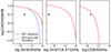
Fig. 15. N2, S2, O1 BPT diagram of the center (black dot with error bars). Theoretical maximum starburst (Kewley et al. 2001) and empirical star formation (Kauffmann et al. 2003) lines are shown in red solid and blue dashed lines respectively.
-
Planetary nebulae: In dense regions close to the central star of planetary nebulae, Lyβ photons can excite neutral oxygen efficiently. Lyβ-pumped O Iλ8449 emission has been observed in several compact, high-density planetary nebulae, such as NGC 7027 (Rudy et al. 1992), IC 5117 (Rudy et al. 2001), and IC 4997 (Rudy et al. 1989; Feibelman et al. 1992). However, due to the hot central star, a highly ionized spectrum is generally observed. The estimated temperature for the central stars of NGC 7027, IC 5117, and IC 4997 is 219 000 K (Zhang et al. 2005), 120 000 K (Hyung et al. 2001), and 47 000–59 000 K (Feibelman et al. 1979), respectively. High-ionization lines such as He II or [Ne V] detected in spectra of planetary nebulae listed above, are not observed in Godzilla.
-
Symbiotic stars: Symbiotic stars refer to binary systems consisting of a cool giant star transferring mass to an accompanied hot star, mostly white dwarfs. Lyβ photons from the hot star can excite neutral oxygen atoms in the surrounding gas and induce Bowen fluorescence. Lyβ-pumped O Iλ8449 emission has been observed in many symbiotic starts such as RR Telescopii (RR Tel) (Thackeray 1955; Damineli 2001), AG Pegasi (AG Peg) (Ciatti et al. 1974; Tomov et al. 2016), V1016 Cygni (V1016 Cyg) (Strafella 1981), HM Sagittae (HM Sge) (Ciatti et al. 1977), and BX Monocerotis (BX Mon) (Anupama et al. 2012). Shore & Wahlgren (2010) also thoroughly examined the O Iλ1302 and O I] λ1641 observed in EG And, Z And, V1016 Cyg, and RR Tel, along with nova RS Oph 1985 in outburst, and concluded that the line strength variation is related to the light curve and outburst activity. Spectra of symbiotic stars listed above all show high-excitation lines including He II originating from hot white dwarfs, which are not observed in Godzilla.
-
Nova ejecta: During a nova eruption, a white dwarf accretes material from its companion star until a thermonuclear runaway occurs. The ejected material is intensely ionized and, as it cools, it produces various emission lines including O Iλ8449. Lyβ-pumped O Iλ8449 has been observed in several novae in the outburst phase, such as nova Cygni 1975 (Strittmatter et al. 1977) and nova V4643 Sgr (Ashok et al. 2006). In their outburst phase, novae typically exhibit high-excitation lines such as He II and O VI, which have not been observed for Godzilla, but which show rapid spectral evolution on a timescale of several days to months.
-
Herbig Ae/Be (HAeBe) Stars: These young, pre-main sequence stars, defined by Herbig (1960), are surrounded by accretion disks. UV radiation from these stars, as well as shocks within the accretion disks, can induce the Bowen fluorescence. Mathew et al. (2018) argued that Lyβ-pumping is the primary mechanism responsible for O Iλ8449 line observed in HAeBe stars. Although HAeBe stars show many spectral similarities to Godzilla, they have less in common compared to η Car and the Weigelt blobs, which is discussed in the next subsection. Figure 2 of Mathew et al. (2018) shows that in HAeBe stars, the O Iλ8449/λ7776 ratio can reach up to about ∼25–50 in extreme cases, whereas in Godzilla, this ratio is ∼110. While O Iλ7776 is fairly prominent in many HAeBe stars, this line is not detected in Godzilla. Furthermore, due to the presence of a stellar disk, Hα in HAeBe stars often shows a double-peak profile, and even when a single peak is present, it lacks the broad wings observed in Godzilla (Carmona et al. 2010, Fig. 3).
5.3.3. LBV – η Car and the Weigelt blobs
We find that the peculiar O Iλ8449 source in Godzilla is best explained as an analog of the Luminous Blue Variable (LBV) star η Car and the Weigelt blobs, given its spectral characteristics. In Section 4.4, we have shown that the strong, narrow permitted oxygen line O Iλ8449 has most likely arisen from a Lyβ pumping mechanism. In Section 5.3.2, we have reviewed a number of known astronomical sources of O Iλ8449 emission, and have shown that the combination of a strong O Iλ8449 line and the absence of the O Iλ7776 line is a rare feature, observed only in Weigelt blobs among objects that do not exhibit high-ionization lines. Moreover, as mentioned in Section 4.3, we know that dense gas of ne ≳ 106 cm−3 exists in close vicinity of Godzilla (Vanzella et al. 2020), although our optical density diagnostics only offer limited constraints on low density gas. Existence of high density gas and the strong fluorescent line emission is evocative of the Weigelt blobs in the η Car systems explained in Section 1.
The Weigelt blobs are dense gas condensations that are primarily neutral, with an ionized surface layer facing the stars (See Figure 1 in Johansson & Letokhov 2005, for a sketched out overview). The O I in the neutral condensations is shielded by hydrogen from ionisation, but exposed to Lyβ photons emitted from the H II surface of the blob, as well as the stellar wind, populating the 3d3D level of the neutral oxygen atoms (Johansson & Letokhov 2005, Figure 4). This level has an excitation energy very close to the resonant energy of Lyβ photons and can be pumped by it, if Lyβ is sufficiently strong – a mechanism known as PAR. Shore & Wahlgren (2010, Figure 1) show a different view of this same cascade. Once the 3d3D level is populated, it decays to 3p3P level through a λ = 11286 Å transition which is outside the wavelength range of these observations. Subsequently, they continue to cascade down from 3p3P to 3s3S1 through the λ = 8449 Å transition, and from there into O I]λ1641 and the λ = 1302, 1304, 1306 triplet. We note that all of these lines are strongly detected in the MagE and NIRSpec observations of Godzilla. In the Weigelt blobs, as oxygen in the interior of the blob remains neutral, it results in a special situation where we observe strong Lyβ-pumped O Iλ8449, but not the recombination line O Iλ7776. The clear detection of the full Lyβ-pumped cascade, combined with the non-detection of O Iλ7776 (Section 4.4, Figure 9) is the smoking gun that permitted O I lines in Godzilla has arisen from dense, Weigelt blob-like gas condensations.
In the Weigelt blobs, [Ne III] is only observed at times when the blob is exposed to the secondary star, which is hotter than the LBV star. We can explain the significant dust attenuation, the strong Bowen fluorescent emission, and the [Ne III] emission line simultaneously, if Godzilla is a binary system including a massive evolved LBV-like star and a hotter star, analogous to η Car. It is a plausible scenario considering that 70% of massive stars are affected by binary interaction, and 50% have companions (Weis & Bomans 2020). It is also noteworthy that Smith & Tombleson (2015) and Smith (2019) suggested that LBVs result from close binary evolution. Alternatively, the properties listed above can be explained without invoking a binary scenario, if the gas condensations in Godzilla are exposed to more intense radiation of an LBV star compared to the Weigelt blobs. Assuming the LBV star has a similar temperature to η Car, this would be possible if the blobs were located more closely to the star than the Weigelt blobs to η Car. These two scenarios could potentially be distinguished by observing periodic variability in line emission. However, depending on the inclination and viewing angle, spectral variability might not be detected, even if it is indeed a binary system.
We would also like to discuss the magnification and brightness issues raised in previous studies. Diego et al. (2022) has noted that with μ ≈ 7000, the true brightness of Godzilla would match that of η Car during its great eruption. Despite the high resolution of JWST/NIRSpec, we do not detect any signs of an eruption such as a very broad Hα (∼104 km s−1) or P Cygni profiles. If we adopt the values suggested by Diego et al. (2022), this implies that the magnification factor for Godzilla must exceed 7000 if the source has the same magnitude as η Car in its non-eruption phase. However, it should be noted that the analysis by Diego et al. (2022) is based on the assumption that Godzilla is a single stellar source. If Godzilla is indeed composed of multiple stars, the constraints on the magnification factor could be relaxed.
The overall picture we propose is as follows: Godzilla is part of clump 4, comprising 10–25% of its stellar light, depending on the lens models and the images in comparison. It could be a small group of just a few stars, or tens or even hundreds of stars. These stars contribute significant or even dominating fraction of the stellar continuum. Within this group of stars, a peculiar O Iλ8449 source is present, which is best explained as a source similar to the Weigelt blobs in the η Car system. The spectra of Godzilla resemble those of η Car in its quiescent phase, with nearby dense gas condensations exposed to a hotter source, either due to a presumable hotter companion or their potentially closer location to the star. We believe that the emission lines observed in Godzilla are primarily from this dense gas condensation, though some lines, such as redshifted [O II] lines, may originate from other regions (Figure 8). Our scenario is a kind of hybrid model, differing from both Diego et al. (2022)’s interpretation of Godzilla as a single object and Pascale & Dai (2024)’s interpretation as a star cluster, in the sense that the stellar continuum is affected by multiple stars, while a single object analogous to η Car dominates the emission line. In the next section, we further examine the similarities and differences between O Iλ8449 in Godzilla and the Weigelt blobs.
5.4. Comparison to Bowen fluorescent lines observed in η Carinae
5.4.1. A possible astronomical laser effect
Johansson & Letokhov (2005) discuss the possibility of astrophysical laser effects of O Iλ8449 in the Weigelt blobs. As the decay of the lower 3s3S1 level to the ground level is faster than the decay of the upper 3p3P level, population inversion occurs. O Iλ8449 from Godzilla is due to Lyβ pumping, so we expect it to show an inverted population, but it does not necessarily mean that it is a laser since we cannot guarantee stimulated emission without information on the size of the blob and amplification of the O Iλ8449 line. To obtain an observational confirmation, Johansson & Letokhov (2005) suggested looking for sub-Doppler width (i.e., the line width narrower than the width caused by Doppler broadening) of the 8449 line.
Lyα-pumped iron lines can provide us an additional clue about the sub-Doppler width of the O Iλ8449 line. Along with the Lyβ-pumped O Iλ8449, we detect Lyα-pumped Fe IIλ8490 with an S/N of 8 (see Table A.2). Interestingly, another Lyα-pumped iron line, Fe IIλ8453, which arise from the same mechanism thus should appear is not detected in the fits using [O III]λλ4960,5008 as kinematic template (Table A.2). This line is blended with O Iλ8449, and we suspect that its flux may have been included in the O Iλ8449 flux since the O Iλ8449 line is narrower than other lines. We fitted the fluorescent lines again, using only one component and relaxing the width constraint. The result is shown in Table A.2 with asterisk. We measured FWHM of 106 ± 5 km s−1 for the fluorescent lines and it increased the S/N of Fe IIλ8453 from ∼1.8 to ∼12. However, along with the lack of information on the thermal broadening in this object, the spectral resolution of NIRSpec does not allow sufficiently strong constraints on the line profile to confirm or falsify if the O Iλ8449 emission observed in Godzilla is an astronomical laser.
5.4.2. Flux discrepancy in Lyα-pumped lines
The relative strengths of Lyα-pumped Fe II lines compared to the Lyβ-pumped O Iλ8449 line is significantly smaller than observed in the Weigelt blobs (see Davidson & Humphreys 2012, Figure 5.4). In the Weigelt blobs, Fe II fluorescent lines are much stronger than O Iλ8449. This might imply an abundance difference, which is not surprising considering that Godzilla is at z = 2.37 and the Weigelt blobs are in our Galaxy, where the metal enrichment has been enhanced by Type Ia SN. Several observations have already suggested significant alpha enhancement, that is, an iron deficiency, in z ∼ 2 − 3 galaxies (Steidel et al. 2016; Topping et al. 2020a,b; Cullen et al. 2021). Alternatively, it might be a circumstantial evidence of a O I laser and significant amplification in that line.
6. Conclusions
We report the results from Cycle 1 JWST/NIRCam and NIRSpec observations of the object nick-named “Godzilla” in the Sunburst Arc. The Sunburst Arc is the brightest known gravitationally lensed galaxy at z = 2.37 and consists of 12 full or partial images of the source galaxy. Godzilla only appears in one of these, although it does stand out one of the brightest elements of that particular image. While the absence of counterimages of Godzilla has been explained on the basis of extreme magnification (Diego et al. 2022; Sharon et al. 2022), there is an ongoing debate on the nature of the object (Vanzella et al. 2020; Pascale & Dai 2024). It has been suggested that Godzilla might be a rare stellar object called a luminous blue variable (LBV) based on the detection of uncommon Bowen fluorescent lines (Vanzella et al. 2020) and luminosity constraints from the lens model (Diego et al. 2022). However, ground-based telescope observations from previous studies do not have an adequate level of spatial resolution to test this at such a high redshift. In this work, we have extracted the integrated spectra of Godzilla from NIRSpec IFU spaxels containing the central bright object (center) and four regions (NE, SE, NW, SW) surrounding it (Figure 3). We measured the flux of emission lines using one to three component Gaussian profiles depending on the regions and lines. Our main findings are as follows.
-
We detected 57 emission lines from JWST/NIRSpec spectrum of the bright central region (center), listed in Tables A.1 and A.2, including the auroral lines of four species ([N II]λ5756, [O II]λλ7322,7332, [O III]λ4363, and [S III]λ6314), and strong permitted O Iλ8449.
-
NIRCam observations extend the baseline of observations of Godzilla to ∼1.5 years in the rest frame; the source has an approximately flat light curve over that time span and no counterimages have been detected, strengthening the case against the Type IIn supernova scenario or any similarly short-lived transient event (Figure 2). An emission line profile comparison between Godzilla, the P knots (a pair of small clumps next to Godzilla) and the LCE (Figure 10) supports the microlensing scenario suggested by Diego et al. (2022). We suggest a newly detected low-surface brightness galaxy near Godzilla (Figure 11) as a possible perturber, creating the critical curve crossing on top of Godzilla. We agree that Godzilla only appears at its current position since it is extremely magnified (Section 5.1).
-
Based on the similarity in color (Figure 12) and the strong O Iλ8449 emission (Figure 13), we concluded that the images of clump 4 do contain Godzilla. We compared the flux of the stellar continuum and the O Iλ8449 emission line between Godzilla and the clump 4 images (Table 2). Compared to images 4.4 and 4.9, while Godzilla is 35 times and 94 times brighter in O Iλ8449, it is only 8 and 10 times brighter in the continuum, respectively. This implies that Godzilla contains 10–25% of the total stellar light of the clump 4 (Figure 14). Depending on the lens models used, the magnification factor of Godzilla can vary widely, ranging from ≈600 to ≈25 000.
-
We have shown that O Iλ8449 is most likely produced through Lyβ-pumping (Section 4.4). We report the UV counterpart of the Lyβ-pumped O I triplet detected in a Magellan/MagE spectrum, along with O I]λ1641 (Figure 9). By examining possible scenarios (Section 5.3.2), we conclude that the presence of this Lyβ-pumped cascade implies the existence of dense gas condensations in close vicinity of the energy source, which is analogous to the Weigelt blobs near Eta Carinae (η Car), an LBV star in the Milky Way (Section 5.3.3). This conclusion is in line with the previous detection of Lyα-pumped Bowen lines (Vanzella et al. 2020). In this work, we also discuss the hypothesized natural laser effect in O Iλ8449, which was previously suggested in the literature (Johansson & Letokhov 2005). However, while we find the suggestion to be plausible, we do not find any basis in the data to confirm or refute a contribution to the line emission from such a natural laser (Section 5.4).
-
Godzilla and the surrounding regions are very dusty (Table 3) and the broadest component shows a moderately high velocity dispersion of 435–547 km s−1 (Table 1). Based on spatially varying line profiles (Figure 3), dust reddening, temperature, and density (Figure 8, Figure C.2), as well as velocity, we postulate that this object is surrounded by multi-phase circumstellar or interstellar medium.
-
We find that an LBV with a hotter companion (analogous to η Car) would best explain our observations simultaneously and in a qualitative sense, while requiring the least extreme magnification. Gas condensation located more closely to the source, which is exposed to the harder radiation, compared to the Weigelt blobs, could stand as an alternative scenario. Considering (1) the fact that the measured maximum velocity of the broadest component of Hα in Godzilla is an order of magnitude smaller than that of η Car during the great eruption (Figure 6, Section 4.2) and (2) the non-detection of P Cygni profiles, we conclude that the source is not undergoing an eruption phase. A spectroscopic monitoring program of Godzilla might help determine whether there is some periodic variation in the nebular emission lines, such as the 5.54-year spectroscopic period seen for η Car; however, we note that the variation effect could be highly affected by the inclination and viewing angle.
Godzilla is a truly remarkable object. In addition to existing clues in the literature, we find strong spectroscopic evidence pointing to the object containing an η Car analog, with very dense, neutral gas condensations exposed to more intense emission, and possibly accompanied by a smaller, hot, blue companion. Future investigations of possible spectral variability and refined lens models may help further constrain the true nature of Godzilla.
Martin, J., 2024, Observations from the AAVSO International Database, https://www.aavso.org
Acknowledgments
The authors would like to thank Seán Brennan, Ragnhild Lunnan and Yang Hu, Stockholm University, for helpful discussions about late stage evolution of massive stars. This work is in part based on observations made with the NASA/ESA/CSA James Webb Space Telescope. The data were obtained from the Mikulski Archive for Space Telescopes at the Space Telescope Science Institute, which is operated by the Association of Universities for Research in Astronomy, Inc., under NASA contract NAS 5-03127 for JWST. These observations are associated with program #2555. Support for program #2555 was provided by NASA through a grant from the Space Telescope Science Institute, which is operated by the Association of Universities for Research in Astronomy, Inc., under NASA contract NAS 5-03127. ER-T is supported by the Swedish Research Council grant Nr. 2022-04805_VR. This work makes use of the software packages Astropy (Astropy Collaboration 2013, 2018, 2022), Matplotlib (Hunter 2007), NumPy (Harris et al. 2020), Uncertainties Python package by Eric O. LEBIGOT, Jupyter notebook (Kluyver et al. 2016), LMFIT (Newville et al. 2014) and PyNeb (Luridiana et al. 2015).
References
- Abraham, Z., Falceta-Gonçalves, D., & Beaklini, P. P. B. 2014, ApJ, 791, 95 [NASA ADS] [CrossRef] [Google Scholar]
- Abraham, Z., Beaklini, P. P. B., Cox, P., Falceta-Gonçalves, D., & Nyman, L.-Å. 2020, MNRAS, 499, 2493 [Google Scholar]
- Allen, D. A., & Swings, J. P. 1976, A&A, 47, 293 [NASA ADS] [Google Scholar]
- Anupama, G. C., Kamath, U. S., Gurugubelli, U. K., & Mikołajewska, J. 2012, Open Astron., 21, 172 [Google Scholar]
- Ashok, N. M., Banerjee, D. P. K., Varricatt, W. P., & Kamath, U. S. 2006, MNRAS, 368, 592 [Google Scholar]
- Astropy Collaboration (Robitaille, T. P., et al.) 2013, A&A, 558, A33 [NASA ADS] [CrossRef] [EDP Sciences] [Google Scholar]
- Astropy Collaboration (Price-Whelan, A. M., et al.) 2018, AJ, 156, 123 [Google Scholar]
- Astropy Collaboration (Price-Whelan, A. M., et al.) 2022, ApJ, 935, 167 [NASA ADS] [CrossRef] [Google Scholar]
- Bowen, I. S. 1934, PASP, 46, 146 [NASA ADS] [CrossRef] [Google Scholar]
- Bradley, L., Sipőcz, B., Robitaille, T., et al. 2024, https://doi.org/10.5281/Zenodo.596036 [Google Scholar]
- Calzetti, D., Armus, L., Bohlin, R. C., et al. 2000, ApJ, 533, 682 [NASA ADS] [CrossRef] [Google Scholar]
- Carmona, A., Van Den Ancker, M. E., Audard, M., et al. 2010, A&A, 517, A67 [NASA ADS] [CrossRef] [EDP Sciences] [Google Scholar]
- Chen, W., Kelly, P. L., Diego, J. M., et al. 2019, ApJ, 881, 8 [NASA ADS] [CrossRef] [Google Scholar]
- Ciatti, F., D’Odorico, S., & Mammano, A. 1974, A&A, 34, 181 [Google Scholar]
- Ciatti, F., Mammano, A., & Vittone, A. 1977, A&A, 61, 459 [Google Scholar]
- Conti, P. S. 1984, Obs. Tests Stellar Evol. Theory, 105, 233 [Google Scholar]
- Cullen, F., Shapley, A. E., McLure, R. J., et al. 2021, MNRAS, 505, 903 [CrossRef] [Google Scholar]
- Dahle, H., Aghanim, N., Guennou, L., et al. 2016, A&A, 590, L4 [NASA ADS] [CrossRef] [EDP Sciences] [Google Scholar]
- Damineli, A. 1996, ApJ, 460, L49 [NASA ADS] [Google Scholar]
- Damineli, A. 2001, Eta Carinae Mysterious Stars Hidden Oppor. Emiss. Spectrosc., 242, 203 [Google Scholar]
- Davidson, K., & Humphreys, R. M. 2012, in Eta Carinae and the Supernova Impostors (Boston, MA: Springer, US), Astrophys. Space Sci. Libr., 384 [CrossRef] [Google Scholar]
- Davidson, K., Ebbets, D., Weigelt, G., et al. 1995, ApJ, 109, 1784 [Google Scholar]
- de Groot, M. 1988, Ir. Astron. J., 18, 163 [NASA ADS] [Google Scholar]
- de Winter, D., & van den Ancker, M. E. 1997, A&AS, 121, 275 [NASA ADS] [CrossRef] [EDP Sciences] [Google Scholar]
- Diego, J. M. 2019, A&A, 625, A84 [NASA ADS] [CrossRef] [EDP Sciences] [Google Scholar]
- Diego, J. M., Kaiser, N., Broadhurst, T., et al. 2018, ApJ, 857, 25 [NASA ADS] [CrossRef] [Google Scholar]
- Diego, J. M., Pascale, M., Kavanagh, B. J., et al. 2022, A&A, 665, A134 [NASA ADS] [CrossRef] [EDP Sciences] [Google Scholar]
- Diego, J. M., Meena, A. K., Adams, N. J., et al. 2023a, A&A, 672, A3 [NASA ADS] [CrossRef] [EDP Sciences] [Google Scholar]
- Diego, J. M., Sun, B., Yan, H., et al. 2023b, A&A, 679, A31 [NASA ADS] [CrossRef] [EDP Sciences] [Google Scholar]
- Draine, B. T. 2011, Physics of the Interstellar and Intergalactic Medium (Princeton University Press) [Google Scholar]
- Feibelman, W. A., Hobbs, R. W., McCracken, C. W., & Brown, L. W. 1979, ApJ, 231, 111 [NASA ADS] [CrossRef] [Google Scholar]
- Feibelman, W. A., Aller, L. H., & Hyung, S. 1992, PASP, 104, 339 [NASA ADS] [CrossRef] [Google Scholar]
- Fernández-Lajús, E., Fariña, C., Torres, A. F., et al. 2009, A&A, 493, 1093 [NASA ADS] [CrossRef] [EDP Sciences] [Google Scholar]
- Fudamoto, Y., Sun, F., Diego, J. M., et al. 2025, Nat. Astron., 9, 428 [Google Scholar]
- Furtak, L. J., Meena, A. K., Zackrisson, E., et al. 2024, MNRAS, 527, L7 [NASA ADS] [Google Scholar]
- Grandi, S. A. 1975, ApJ, 196, 465 [NASA ADS] [CrossRef] [Google Scholar]
- Grandi, S. A. 1980, ApJ, 238, 10 [NASA ADS] [CrossRef] [Google Scholar]
- Guseva, N. G., Thuan, T. X., & Izotov, Y. I. 2023, MNRAS, 527, 3932 [NASA ADS] [CrossRef] [Google Scholar]
- Haisch, B. M., Linsky, J. L., Weinstein, A., & Shine, R. A. 1977, ApJ, 214, 785 [Google Scholar]
- Hamann, F., Davidson, K., Ishibashi, K., & Gull, T. R. 1999, Eta Carinae Millenn., 179, 166 [Google Scholar]
- Harris, C. R., Millman, K. J., Van Der Walt, S. J., et al. 2020, Nature, 585, 357 [NASA ADS] [CrossRef] [Google Scholar]
- Herbig, G. H. 1960, ApJS, 4, 337 [Google Scholar]
- Herrero, A., Garcia, M., Uytterhoeven, K., et al. 2010, A&A, 513, A70 [NASA ADS] [CrossRef] [EDP Sciences] [Google Scholar]
- Humphreys, R. M., Davidson, K., & Smith, N. 1999, PASP, 111, 1124 [NASA ADS] [CrossRef] [Google Scholar]
- Hunter, J. D. 2007, Comput. Sci. Eng., 9, 90 [NASA ADS] [CrossRef] [Google Scholar]
- Hyung, S., Aller, L. H., Feibelman, W. A., & Lee, S.-J. 2001, ApJ, 563, 889 [NASA ADS] [CrossRef] [Google Scholar]
- Immler, S., Fesen, R. A., Van Dyk, S. D., et al. 2005, ApJ, 632, 283 [Google Scholar]
- Itoh, H. 1986, PASJ, 38, 717 [Google Scholar]
- Jaschek, M., Slettebak, A., & Jaschek, C. 1981, Be Star Newsletter, 4, 9 [Google Scholar]
- Johansson, S., & Letokhov, V. S. 2005, MNRAS, 364, 731 [NASA ADS] [Google Scholar]
- Kauffmann, G., Heckman, T. M., Tremonti, C., et al. 2003, MNRAS, 346, 1055 [Google Scholar]
- Kaurov, A. A., Dai, L., Venumadhav, T., Miralda-Escudé, J., & Frye, B. 2019, ApJ, 880, 58 [NASA ADS] [CrossRef] [Google Scholar]
- Kelly, P. L., Diego, J. M., Rodney, S., et al. 2018, Nat. Astron., 2, 334 [NASA ADS] [CrossRef] [Google Scholar]
- Kelly, P. L., Chen, W., Alfred, A., et al. 2022, ArXiv e-prints [arXiv:2211.02670] [Google Scholar]
- Kewley, L. J., Dopita, M. A., Sutherland, R. S., Heisler, C. A., & Trevena, J. 2001, ApJ, 556, 121 [Google Scholar]
- Kewley, L. J., Nicholls, D. C., & Sutherland, R. S. 2019, ARA&A, 57, 511 [Google Scholar]
- Khatami, D. K., & Kasen, D. N. 2024, ApJ, 972, 140 [NASA ADS] [CrossRef] [Google Scholar]
- Kluyver, T., Ragan-Kelley, B., Pérez, F., et al. 2016, in Jupyter Notebooks–a Publishing Format for Reproducible Computational Workflows, 87 [Google Scholar]
- Kogure, T., & Leung, K.-C. 2007, The Astrophysics of Emission-Line Stars, Astrophysics and Space Science Library (New York: Springer), 342 [CrossRef] [Google Scholar]
- Kramida, A., & Ralchenko, Y. 1999, NIST Atomic Spectra Database, NIST Standard Reference Database, 78 [Google Scholar]
- Luridiana, V., Morisset, C., & Shaw, R. A. 2015, A&A, 573, A42 [NASA ADS] [CrossRef] [EDP Sciences] [Google Scholar]
- Mainali, R., Rigby, J. R., Chisholm, J., et al. 2022, ApJ, 940, 160 [NASA ADS] [CrossRef] [Google Scholar]
- Makarov, D. I., Makarova, L. N., Pustilnik, S. A., & Borisov, S. B. 2017, MNRAS, 466, 556 [CrossRef] [Google Scholar]
- Mathew, B., Banerjee, D. P. K., Naik, S., & Ashok, N. M. 2012a, MNRAS, 423, 2486 [CrossRef] [Google Scholar]
- Mathew, B., Banerjee, D. P. K., Subramaniam, A., & Ashok, N. M. 2012b, ApJ, 753, 13 [NASA ADS] [CrossRef] [Google Scholar]
- Mathew, B., Manoj, P., Narang, M., et al. 2018, ApJ, 857, 30 [NASA ADS] [CrossRef] [Google Scholar]
- Mauerhan, J. C., Smith, N., Silverman, J. M., et al. 2013, MNRAS, 431, 2599 [Google Scholar]
- Meena, A. K., Zitrin, A., Jiménez-Teja, Y., et al. 2023, ApJ, 944, L6 [NASA ADS] [CrossRef] [Google Scholar]
- Mehner, A., Davidson, K., Ferland, G. J., & Humphreys, R. M. 2010, ApJ, 710, 729 [NASA ADS] [CrossRef] [Google Scholar]
- Milisavljevic, D., Fesen, R. A., Chevalier, R. A., et al. 2012, ApJ, 751, 25 [NASA ADS] [CrossRef] [Google Scholar]
- Miralda-Escude, J. 1991, ApJ, 379, 94 [NASA ADS] [CrossRef] [Google Scholar]
- Newville, M., Stensitzki, T., Allen, D. B., & Ingargiola, A. 2014, https://doi.org/10.5281/Zenodo.11813 [Google Scholar]
- Owens, M. R., Kim, K. J., Bayliss, M. B., et al. 2024, ApJ, 977, 234 [Google Scholar]
- Pascale, M., & Dai, L. 2024, ApJ, 976, 166 [Google Scholar]
- Pignataro, G. V., Bergamini, P., Meneghetti, M., et al. 2021, A&A, 655, A81 [NASA ADS] [CrossRef] [EDP Sciences] [Google Scholar]
- Rigby, J. R., Bayliss, M. B., Sharon, K., et al. 2018, ApJ, 155, 104 [Google Scholar]
- Rivera-Thorsen, T. E., Dahle, H., Gronke, M., et al. 2017, A&A, 608, L4 [NASA ADS] [CrossRef] [EDP Sciences] [Google Scholar]
- Rivera-Thorsen, T. E., Dahle, H., Chisholm, J., et al. 2019, Science, 366, 738 [Google Scholar]
- Rodney, S. A., Balestra, I., Bradac, M., et al. 2018, Nat. Astron, 2, 324 [Google Scholar]
- Rudy, R. J., Rossano, G. S., & Puetter, R. C. 1989, ApJ, 346, 799 [Google Scholar]
- Rudy, R. J., Erwin, P., Rossano, G. S., & Puetter, R. C. 1992, ApJ, 384, 536 [Google Scholar]
- Rudy, R. J., Lynch, D. K., Mazuk, S., Puetter, R. C., & Dearborn, D. S. P. 2001, ApJ, 121, 362 [Google Scholar]
- Sharon, K., Mahler, G., Rivera-Thorsen, T. E., et al. 2022, ApJ, 941, 203 [NASA ADS] [CrossRef] [Google Scholar]
- Shore, S. N., & Wahlgren, G. M. 2010, A&A, 515, A108 [NASA ADS] [CrossRef] [EDP Sciences] [Google Scholar]
- Smith, N. 2019, MNRAS, 489, 4378 [NASA ADS] [CrossRef] [Google Scholar]
- Smith, N., & Ferland, G. J. 2007, ApJ, 655, 911 [NASA ADS] [CrossRef] [Google Scholar]
- Smith, N., & Tombleson, R. 2015, MNRAS, 447, 598 [NASA ADS] [CrossRef] [Google Scholar]
- Smith, N., Rest, A., Andrews, J. E., et al. 2018, MNRAS, 480, 1457 [NASA ADS] [CrossRef] [Google Scholar]
- Solhaug, E., Chen, H. W., Chen, M. C., et al. 2025, Open J. Astrophys., 8, 35 [Google Scholar]
- Steidel, C. C., Strom, A. L., Pettini, M., et al. 2016, ApJ, 826, 159 [NASA ADS] [CrossRef] [Google Scholar]
- Strafella, F. 1981, ApJ, 243, 583 [Google Scholar]
- Strittmatter, P. A., Woolf, N. J., Thompson, R. I., et al. 1977, ApJ, 216, 23 [Google Scholar]
- Strom, A. L., Rudie, G. C., Trainor, R. F., et al. 2023, ApJ, 958, L11 [NASA ADS] [CrossRef] [Google Scholar]
- Tachiev, G., & Fischer, C. F. 2001, Can. J. Phys., 79, 955 [NASA ADS] [CrossRef] [Google Scholar]
- Thackeray, A. D. 1955, MNRAS, 115, 236 [Google Scholar]
- Tomov, T. V., Stoyanov, K. A., & Zamanov, R. K. 2016, MNRAS, 462, 4435 [NASA ADS] [CrossRef] [Google Scholar]
- Topping, M. W., Shapley, A. E., Reddy, N. A., et al. 2020a, MNRAS, 499, 1652 [NASA ADS] [CrossRef] [Google Scholar]
- Topping, M. W., Shapley, A. E., Reddy, N. A., et al. 2020b, MNRAS, 495, 4430 [Google Scholar]
- Vanzella, E., Meneghetti, M., Pastorello, A., et al. 2020, MNRAS, 499, L67 [CrossRef] [Google Scholar]
- Venumadhav, T., Dai, L., & Miralda-Escudé, J. 2017, ApJ, 850, 49 [NASA ADS] [CrossRef] [Google Scholar]
- Weigelt, G., & Ebersberger, J. 1986, A&A, 163, L5 [NASA ADS] [Google Scholar]
- Weis, K., & Bomans, D. J. 2020, Galaxies, 8, 20 [NASA ADS] [CrossRef] [Google Scholar]
- Weisenbach, L., Anguita, T., Miralda-Escudé, J., et al. 2024, ArXiv e-prints [arXiv: 2404.08094] [Google Scholar]
- Welch, B., Coe, D., Diego, J. M., et al. 2022a, Nature, 603, 815 [NASA ADS] [CrossRef] [Google Scholar]
- Welch, B., Coe, D., Zackrisson, E., et al. 2022b, ApJ, 940, L1 [NASA ADS] [CrossRef] [Google Scholar]
- Winkler, P. F., & Kirshner, R. P. 1985, ApJ, 299, 981 [NASA ADS] [CrossRef] [Google Scholar]
- Wofford, A., Ramírez, V., Lee, J. C., et al. 2020, MNRAS, 493, 2410 [NASA ADS] [CrossRef] [Google Scholar]
- Wolf, B. 1989, A&A, 217, 87 [NASA ADS] [Google Scholar]
- Zhang, Y., Liu, X. W., Luo, S. G., Péquignot, D., & Barlow, M. J. 2005, A&A, 442, 249 [NASA ADS] [CrossRef] [EDP Sciences] [Google Scholar]
Appendix A: Measured fluxes for the center
Dust-corrected line fluxes for the central G140H/F100LP spectrum.
Measured and dust corrected line fluxes for the central G235H/F170LP spectrum.
Appendix B: Spectral line identification
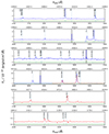 |
Fig. B.1. 1D spectrum from the bright central region of Godzilla. Observed-frame flux densities from the G140H/F100LP and G235H/F170LP gratings are shown in blue and red solid lines, respectively. Standard deviation is shown with green area and hot/noisy pixels are marked with grey shades. |
Appendix C: Properties in surroundings
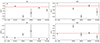 |
Fig. C.1. E(B − V) computed for the NE, SE, NW, and SW regions in the same manner as Figure 7. The red-dashed horizontal lines show the inverse error weighted averages. |
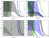 |
Fig. C.2. Joint temperature and density solutions computed with PyNeb for the NE, SE, NW, and SW regions, using the same nebular lines as found in Figure 8. |
Appendix D: O Iλ8449 map normalized by Hβ
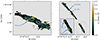 |
Fig. D.1. O Iλ8449/Hβ map for Pointing 1 (left) and Pointings 2+3 (right), with the stellar continuum overlaid as contours. The excess in O I/Hβ is observed in Godzilla, the P knots and the counterimages of the clump 4 as in the [O III] normalization map (Figure 13). |
All Tables
Kinematics information for all regions. NE and SE regions only have narrow components, since we only performed a one-component Gaussian fitting for these regions.
Flux ratio compared to candidate counterimages and the derived magnification factor.
Measured and dust corrected line fluxes for the central G235H/F170LP spectrum.
All Figures
|
Fig. 1. Left: Overview of the north and northwest arc with the NIRSpec IFU pointings overlaid. The cyan, magenta, and yellow squares depict pointings 1, 2, and 3, respectively. We used NIRCam F115W, F200W, and F444W filters for R, G, and B, respectively. Godzilla in pointing 2 is marked with an orange arrow. (right) Pointings 2 and 3 showing Godzilla marked with an orange arrow. The images are oriented such that N is up, E is left. Each combined NIRSpec pointing is approximately |
| In the text | |
|
Fig. 2. Composite of NIRCam F115W, F200W, and F444W images of the north and the northwest arc of the Sunburst Arc. Images 3–10 of clump 4 are marked with purple circles, while images 1–10 of the LyC leaking clump (clump 1) are marked with red squares. In image 8 of clump 4 (4.8), we observe Godzilla and the P knots (the two small clumps). Images 1–4 of clump 5 are marked with green circles. These four images and image 4.7 (t1–t5 in Diego et al. (2022)) have been suggested as candidates for the counterimages of Godzilla by Diego et al. (2022). |
| In the text | |
|
Fig. 3. Five regions where spectra have been extracted and their [O III]λλ4960,5008 doublet line profiles in the G140H/F100LP grating. The center figure shows the wavelength-axis median image of the NIRSpec G140H/F100LP grating at the area of Godzilla. Two-component (center, NW, SW) and one-component (NE, SE) Gaussian fits are also shown. |
| In the text | |
|
Fig. 4. Top: 1D spectrum extracted from the center region, labeled with prominent lines. Bottom: Corrected error from G140H/F100LP and G235H/F170LP gratings shown in blue and red, respectively. Noise pixels are marked with grey shades. Both flux density and errors from the two gratings are overlapped in ∼4925 − 5610 Å. See Figures B.1 and B.2 for more detailed features. |
| In the text | |
|
Fig. 5. Line profiles of Hβ, [O III]5008, and Hα+[N II] of the center region, highlighting the broad component present in Hα but not the other lines. The y-axis scale is linear between –1 and 1, and logarithmic outside this interval. The velocity scale in the lower panel is centered around Hα. |
| In the text | |
|
Fig. 6. Fitting result of Hα including a very broad component additional to default two component (center) and one component (NE, SE) Gaussian profiles. |
| In the text | |
|
Fig. 7. E(B − V) as computed from the strongest Balmer and Paschen lines for the central region. The value from Hα is shown both including and excluding the very broad component. The average weighted by inverse of error is shown in red-dashed horizontal line with a shade representing 1σ uncertainty. Similar figures for the surrounding regions are shown in Figure C.1. |
| In the text | |
|
Fig. 8. Temperature and density solutions from PyNeb for the spectrum extracted from the center region in Figure 3. Oxygen, sulphur, and nitrogen diagnostics are depicted in green, grey, and blue colors, respectively, with shades representing the 1-σ confidence regions. We note that the Te [O II] diagnostic shown here might not be trustworthy, if indeed the [O II]λλ3727,3730 emission has a different region of origin than its auroral counterpart (see Section 3.2, Section 4.3). Similar figures for the surrounding regions are shown in Figure C.2. |
| In the text | |
|
Fig. 9. a,b: Rest-frame UV spectrum of Godzilla from Magellan/MagE (Rigby et al. in prep.), showing the O I triplet and Si II line complex around 1304 Å and O I] 1641 Å. All these O I lines are part of the Lyβ pumped Bowen fluorescence cascade. c: NIRSpec spectrum showing position of the rest-frame optical O I recombination lines and/or stellar continuum excitation cascade triplet around 7776 Å and line complex at around 7990 Å, where we would expect to see line emission if the observed O I cascade were due to recombination or stellar continuum pumping. d: Lyβ-pumped, Bowen fluorescent O I 8449 Å. |
| In the text | |
|
Fig. 10. Selected relative line fluxes from Godzilla, the two P-knots, and for comparison the Lyman Continuum emitter (LCE) knot, highlighting kinematics and relative line strengths. The green shaded interval in the [O II] panel indicates where P2 suffers from contamination from noisy pixels. The spectra were first normalized by their median value, the continuum then subtracted, and the resulting lines all normalized by the integral of [O III] 5008 of each spectrum. |
| In the text | |
|
Fig. 11. Combined NIRCam F115W+F150W image, smoothed by a FWHM = 0.1″Gaussian to bring out low surface brightness details. The dashed ellipsoid marks a low surface brightness galaxy close to Godzilla (larger circle) and the P knots (smaller circles). |
| In the text | |
|
Fig. 12. Color-color diagram using the NIRCam F200W, F277W, and F356W filters. Error bars are shown for each point. In the color-color space, Godzilla (orange pentagon) is positioned closer to the images of clump 4 (purple circles, ‘4.’ in ‘4.X’ has been omitted) and P knots (cyan triangles). Its location is clearly distinguished from that of the images of clump 1 (red squares) and clump 5 (green thin diamonds). |
| In the text | |
|
Fig. 13. O Iλ8449/[O III]λ5008 map for Pointing 1 (left) and Pointings 2+3 (right), with the stellar continuum overlaid as contours. The O Iλ8449/[O III]λ5008 ratio is near zero in the images of clump 1 and is highest in the images of clump 4, Godzilla, and the P knots. Refer to Figure D.1 in the appendix to see the map normalized by Hβ. |
| In the text | |
|
Fig. 14. Illustration explaining the relationships between clump 4, its two counterimages (images 4.4 and 4.9), and Godzilla. The difference between the O Iλ8449 flux ratio and the stellar continuum flux ratio indicates that Godzilla contains only a portion of the stars from clump 4, representing between ∼10 % and ∼25 % of the total stellar light, depending on the model and the image used for comparison. The magnification factor also varies significantly, ranging from ∼560 to ∼6700 (excluding errors). |
| In the text | |
|
Fig. 15. N2, S2, O1 BPT diagram of the center (black dot with error bars). Theoretical maximum starburst (Kewley et al. 2001) and empirical star formation (Kauffmann et al. 2003) lines are shown in red solid and blue dashed lines respectively. |
| In the text | |
|
Fig. B.1. 1D spectrum from the bright central region of Godzilla. Observed-frame flux densities from the G140H/F100LP and G235H/F170LP gratings are shown in blue and red solid lines, respectively. Standard deviation is shown with green area and hot/noisy pixels are marked with grey shades. |
| In the text | |
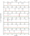 |
Fig. B.2. Same as Figure B.1, continuing to 9300 Å. |
| In the text | |
|
Fig. C.1. E(B − V) computed for the NE, SE, NW, and SW regions in the same manner as Figure 7. The red-dashed horizontal lines show the inverse error weighted averages. |
| In the text | |
|
Fig. C.2. Joint temperature and density solutions computed with PyNeb for the NE, SE, NW, and SW regions, using the same nebular lines as found in Figure 8. |
| In the text | |
|
Fig. D.1. O Iλ8449/Hβ map for Pointing 1 (left) and Pointings 2+3 (right), with the stellar continuum overlaid as contours. The excess in O I/Hβ is observed in Godzilla, the P knots and the counterimages of the clump 4 as in the [O III] normalization map (Figure 13). |
| In the text | |
Current usage metrics show cumulative count of Article Views (full-text article views including HTML views, PDF and ePub downloads, according to the available data) and Abstracts Views on Vision4Press platform.
Data correspond to usage on the plateform after 2015. The current usage metrics is available 48-96 hours after online publication and is updated daily on week days.
Initial download of the metrics may take a while.