| Issue |
A&A
Volume 690, October 2024
|
|
|---|---|---|
| Article Number | A359 | |
| Number of page(s) | 9 | |
| Section | Cosmology (including clusters of galaxies) | |
| DOI | https://doi.org/10.1051/0004-6361/202451246 | |
| Published online | 18 October 2024 | |
A high-resolution view of the source-plane magnification near cluster caustics in wave dark matter models
1
Instituto de Física de Cantabria (CSIC-UC). Avda. Los Castros s/n.
39005
Santander,
Spain
2
Department of Physics, The University of Hong Kong,
Pokfulam Road,
Hong Kong
3
Department of Physics, University of the Basque Country UPV/EHU,
48080
Bilbao,
Spain
4
DIPC, Basque Country UPV/EHU,
48080
San Sebastian,
Spain
5
Ikerbasque, Basque Foundation for Science,
48011
Bilbao,
Spain
6
School of Earth and Space Exploration, Arizona State University,
Tempe,
AZ
85287-6004,
USA
7
Physics Department, Ben-Gurion University of the Negev,
PO Box 653,
Be’er-Sheva
84105,
Israel
8
Department of Astronomy, University of California,
Berkeley,
CA
94720-3411,
USA
9
Minnesota Institute for Astrophysics, University of Minnesota,
116 Church Street SE,
Minneapolis,
MN
55455,
USA
10
School of Physics and Astronomy, University of Minnesota,
116 Church Street,
Minneapolis,
MN
55455,
USA
11
Department of Physics, Oklahoma State University,
145 Physical Sciences Bldg,
Stillwater,
OK
74078,
USA
★ Corresponding author; This email address is being protected from spambots. You need JavaScript enabled to view it.
Received:
25
June
2024
Accepted:
28
August
2024
Abstract
We present the highest-resolution images to date of caustics formed by wave dark matter (ψDM) fluctuations near the critical curves of cluster gravitational lenses. We describe the basic magnification features of ψDM in the source plane at high macromodel magnification and discuss specific differences between the ψDM and standard cold dark matter (CDM) models. The unique generation of demagnified counterimages (with respect to the magnification from the smooth macromodel) formed outside the Einstein radius for ψDM is highlighted. Substructure in CDM cannot generate demagnified images with positive parity and thus does not provide a definitive way to distinguish ψDM from CDM. Highly magnified background sources with sizes r ≈ 1 pc, or approximately a factor of ten smaller than the expected de Broglie wavelength of ψDM, offer the best possibility for discriminating between ψDM and CDM. These include objects such as very compact stellar clusters at high redshift, which JWST is finding in abundance.
Key words: gravitational lensing: strong / dark matter
© The Authors 2024
 Open Access article, published by EDP Sciences, under the terms of the Creative Commons Attribution License (https://creativecommons.org/licenses/by/4.0), which permits unrestricted use, distribution, and reproduction in any medium, provided the original work is properly cited.
This article is published in open access under the Subscribe to Open model. This email address is being protected from spambots. You need JavaScript enabled to view it. to support open access publication.
1 Introduction
The nature of dark matter (DM) is arguably one of the biggest mysteries in modern physics. The cold DM (CDM) model successfully explains the observations on large scales, from galaxy surveys (Alam et al. 2021; Abbott et al. 2022; DESI Collaboration 2024) to the cosmic microwave background (Planck Collaboration VI 2020). From these observations, the standard cosmological model can be derived with percent precision in its most relevant parameters (Planck Collaboration XIII 2016; Planck Collaboration VI 2020). On smaller scales, differences between predictions based on N-body simulations of CDM and observations have been used as examples that challenge the CDM model, but these discrepancies might be due to insufficient modeling of the complex baryon physics in N-body simulations (Weinberg et al. 2015). Perhaps the biggest challenge to CDM resides in the lack of direct confirmation from any of the multiple experiments on Earth. In particular, the continuing search for weakly interacting massive particles (WIMPs) is quickly exhausting the still available space of parameters where long-sought WIMPs were originally expected to be found. This absence of direct confirmation has promoted the appearance of challengers to the CDM model. Among these, wave DM (ψDM Press et al. 1990; Widrow & Kaiser 1993; Peebles 2000; Hu et al. 2000; Schive et al. 2016) has recently attracted attention as an alternative model that can simultaneously explain the large-scale structure of the Universe, the alleged small-scale departures from the CDM expectations, and the lack of success in direct search experiments.
There are other scenarios in which DM physics, or various baryonic effects (e.g., Ragagnin et al. 2024), alter the properties of halos. For example, warm DM models predict less substructure on subgalactic scales. Surviving halos in warm DM have lower concentrations than their CDM counterparts, and therefore have a suppressed lensing efficiency, decreasing the contribution from millilenses to the probability of high magnification (Enzi et al. 2021). On the other hand, self-interacting DM can cause halos to undergo core collapse, a process that dramatically raises their central density, potentially to a degree that causes them to become supercritical for lensing (Gilman et al. 2021). Alternatively, ψDM is expected to increase the magnification in regions relatively far from cluster critical curves (CCs), by producing smaller CCs around the largest ψDM fluctuations (Amruth et al. 2023; Broadhurst et al. 2024).
In ψDM, the DM particle is incredibly light (with a mass ~15 orders of magnitude smaller than that of the classic axion in quantum chromodynamics, for an axion-photon coupling constant of ~10−17 GeV−1) (Hui 2021). In this work, we assume that the DM becomes a Bose-Einstein condensate. In this case, the DM mass is the only free parameter, and the self-interaction and axion-like-particle (ALP) decay can be neglected. The small mass in ψDM results in the distinctive behavior of the DM fluctuations on small scales (<1 kpc), while on megaparsec (Mpc) scales, both ψDM and CDM models predict similar structures (Schive et al. 2014). With its small mass, ψDM behaves as a quantum fluid with a de Broglie wavelength on parsec (pc) to kiloparsec (kpc) scales. Interference of the ψDM fluid results in constructive and destructive interference, where locally the density contrast can have variations of order unity, Δρ/ρ ≈ 1 (Schive et al. 2014). When projecting these large density perturbations along the line of sight, the resulting fluctuations in the projected surface mass density are smaller but still present (by the central limit theorem) (Chan et al. 2020; Amruth et al. 2023). However, these small fluctuations are enhanced near the CCs of massive lenses and leave their mark in background objects through distortions in the magnification. These distortions extend over scales that are comparable to λdB, the de Broglie wavelength of ψDM. Hence, objects that have sizes comparable to λdB can experience differential magnification, depending on whether their counter-images are aligned with a region in the lens having slightly more or less interference. This pervasive interference substructure causes the CCs to become corrugated on the de Broglie scale (Chan et al. 2020; Laroche et al. 2022; Amruth et al. 2023; Powell et al. 2023; Liu et al. 2024), and increasingly so for more massive halos, with many detached islands where the magnification diverges at relatively large offsets from the cluster CCs (Amruth et al. 2023; Laroche et al. 2022).
Recently, ψDM has been tested with observations of lensed objects, such as quasars (Amruth et al. 2023; Powell et al. 2023). The results are inconclusive, with some observations favoring ψDM (Amruth et al. 2023) while others disfavor it (Powell et al. 2023). New observations of distant objects with the James Webb Space Telescope (JWST) are providing a wealth of small but luminous objects that can, in principle, be used in similar studies to test DM models, including ψDM. To perform these tests, a key issue is to understand the magnification properties in different models. For CDM (and its substructure), there is abundant literature exploring the magnification near the CCs of clusters. For ψDM, the literature is scarcer.
One of the limitations of earlier work on the magnification from ψDM is the relatively low resolution, which does not allow the ψDM caustics in the source plane to be properly resolved. Resolving the caustics from ψDM is particularly challenging near the CCs of clusters, where the macromodel magnification is μ > 100. To simulate a region in the source plane of 100 × 100 pc2, the corresponding area in the image plane needs to be over 100 times larger, with the pixel size small enough to resolve the small caustics.
This paper aims to address this issue and provide the first very high resolution view of the ψDM caustics in the source plane, and to study the probability of magnification in the source plane of the ψDM model.
The paper is organized as follows. In Sec. 2, we briefly introduce key concepts in ψDM models. The simulations of the magnification produced by ψDM are discussed in Sec. 3. Section 4 shows the resulting magnification (and its probability distribution) in the image plane and as a function of macromodel magnification. Section 5 then shows the corresponding magnification pattern and probability in the source plane. We discuss our results in Sec. 6 and conclude in Sec. 7. A flat cosmological model was adopted with Ωm = 0.3 and H0 = 70 km s−1 Mpc−1. For our simulations, we assumed a lens at redshift z = 0.4 and a source at z = 1. Our results have a weak dependence on this choice.
Several lensing terms are used through this work, which for the benefit of the nonexpert reader, we introduce here. The projected mass of the lens along the line of sight is usually referred to as the convergence κ, defined as the surface mass density in units of the critical surface mass density, κ = ∑/∑crit. Gravitational lenses contain regions of maximum magnification referred to as critical curves (CCs) where the magnification can reach very large values (≫ 100 for small sources). Two types of CCs are defined: radial CC near the center of the lens and tangential CCs farther away. In this work, we have focused on magnified objects that form near the tangential CC which, in the case of circularly symmetric lenses, is a circle centered on the lens and with radius equal to the Einstein radius. Near the tangential CC, and for smooth models, a source produces two counterimages. One counterimage forms in the interior of the CC. This counter-image is a distorted (stretched) but mirrored image of the original source and usually is referred to as the counterimage with negative parity. A similarly distorted image forms outside the CC but with the same orientation as the original image. This external counterimage is said to have positive parity. Alternatively, we refer to the interior region of the CC as the side with negative parity, while the exterior region is the side with positive parity. We use the term macromodel to refer to the smooth lens model from the galaxy cluster. In the CDM case, the macromodel is assumed to be directly a smooth model, such as a Navarro-Frenk-White (NFW) model (Navarro et al. 1996). In ψDM, the macromodel is similar to the CDM case after the small-scale perturbations from ψDM are smoothed out on sufficiently large scales (larger than the de Broglie wavelength), hence becoming similar to the CDM macromodel. The particular choice of macromodel is not relevant for this work, as our scope is limited to very small scales, where the average macromodel properties can be considered as a constant and fully characterized by the macromodel magnification. On sufficiently small scales, such as those studied in this work, the deflection field of the macromodel can be fully characterized by the values of the tangential and radial magnification, respectively μt and μr, as described in Sect. 3.2 of Diego et al. (2018). Finally, we use the term demagnification to refer to the magnification with respect to the macromodel value, that is, the one that would have been obtained at the same location but without substructure in the case of CDM, or before adding the small-scale perturbations in ψDM.
2 Wave dark matter
In this model, DM has density fluctuations at scales given by the de Broglie wavelength and the halo mass (Schive et al. 2016), from the dependence on momentum,
![Mathematical equation: $\[\lambda_{\mathrm{dB}}=15\left(\frac{10^{-22} ~\mathrm{eV}}{m_\psi}\right)\left(\frac{10^{15} ~\mathrm{M}_{\odot}}{M_{\text {cluster }}}\right)^{1 / 3} \mathrm{pc},\]$](/articles/aa/full_html/2024/10/aa51246-24/aa51246-24-eq1.png) (1)
(1)
where mψ is the mass of the ultralight axion-like particle. For ALP masses mψ ≈ 10−22 eV and a 1015 M⊙ cluster, this scale corresponds to 3 milliarcseconds (mas) in the lens plane (assuming zlens ≈ 0.4).
Similarly to microlenses (typically stars in the intracluster medium), ψDM fluctuations are ubiquitous across the lens plane, and as in the case of microlenses and millilenses (globular clusters and dwarf galaxies in the cluster), these fluctuations get amplified near the CC by the macromodel. The one main difference between ψDM and other small perturbations in the deflection field in the CDM scenario (mostly microlenses and millilenses) is that ψDM perturbations can be either positive or negative in mass (or convergence), while in CDM the perturbations in the mass are always positive1. This difference has profound implications for the resulting probability of magnification, as we discuss in other sections of this paper.
In this work, we were interested in studying the caustics produced by ψDM fluctuations. To gain basic understanding that would be useful in exploring a full simulation, we first studied a simple toy model. The ψDM fluctuations are the result of projecting along the lens’s line of sight the individual granules with positive or negative underdensities (δρ/ρ ≈ 1). If the amplitude of the fluctuations of the individual granules can be described as a random Gaussian field with dispersion σg, their projection is also a Gaussian random field but with a dispersion that scales as ![Mathematical equation: $\[\sqrt{N_g} \sigma_g\]$](/articles/aa/full_html/2024/10/aa51246-24/aa51246-24-eq2.png) , where Ng is the number of granules that are projected along the line of sight. The mean projected signal (or mean of the Gaussian distribution) scales as
, where Ng is the number of granules that are projected along the line of sight. The mean projected signal (or mean of the Gaussian distribution) scales as ![Mathematical equation: $\[\sigma_s / \sqrt{N_g}\]$](/articles/aa/full_html/2024/10/aa51246-24/aa51246-24-eq3.png) by virtue of the central limit theorem, and converges to the total projected mass, which is similar in both CDM and ψDM, except in the very central region of the cluster where the ψDM soliton produces cores (see Schive et al. 2016). We were interested in regions near the cluster CCs and, hence, far from the soliton core. The lensing deflection field from the projected ψDM granules is also a Gaussian field with fluctuations that can be well described by 2D Gaussian functions with full width half maximum intensity (FWHM) comparable in size to the de Broglie wavelength. This configuration is typical of convergence (or mass) fields with continuous positive and negative fluctuations (with respect to the mean) and a similar pattern for the shear (except this is rotated by 90° with respect to the convergence field).
by virtue of the central limit theorem, and converges to the total projected mass, which is similar in both CDM and ψDM, except in the very central region of the cluster where the ψDM soliton produces cores (see Schive et al. 2016). We were interested in regions near the cluster CCs and, hence, far from the soliton core. The lensing deflection field from the projected ψDM granules is also a Gaussian field with fluctuations that can be well described by 2D Gaussian functions with full width half maximum intensity (FWHM) comparable in size to the de Broglie wavelength. This configuration is typical of convergence (or mass) fields with continuous positive and negative fluctuations (with respect to the mean) and a similar pattern for the shear (except this is rotated by 90° with respect to the convergence field).
We simulated one of these Gaussian projected fluctuations and embedded it in a macromodel lensing potential at some small distance, d, from the cluster CC and with macromodel magnifications μ = ±100 × 1.6. The two signs accounted for the two parities, and we fixed the radial magnification to μr = 1.6, since this varies very slowly near cluster CCs. Thus, we simulated the same ψDM fluctuation on both sides of the cluster CC but at a similar distance from the CC, so the macromodel magnification was the same in both parities (but with different signs).
For the ψDM fluctuation, we chose a small scale of just 2 pc, but this is irrelevant because our study of this toy model focused only on the morphology of the caustic, not its scale The resulting caustics are shown in Fig. 1 for the two parities.
At first, the caustics appeared identical for both parities, but on closer inspection we observed a very small shift in the position of the caustics. Ignoring this small shift (much smaller than the de Broglie wavelength), we could conclude that the magnification properties were identical on both sides of the lens CC. In earlier work, Amruth et al. (2023) found a preference for images with negative parity to be less magnified, but in that case the macromodel lens was a galaxy, not a cluster, where, at short distances from the CC, the magnification changes more rapidly with distance for images having negative parity. For clusters, the assumption that the magnification is the same at short distances (d < 1″) from the CC is a much better approximation. This is a unique feature of ψDM substructure, since any other substructure in CDM (positive with respect to the background by definition) results in significant differences in the probability of magnification between the sides with negative and positive parities (see, e.g., Diego et al. 2018; Williams et al. 2024). For instance, substructures in CDM in regions with negative parity can demagnify by a significant amount (with respect to the magnification that would have been obtained without substructure), rendering small objects that fall within the demagnification region undetectable. To compensate for the demagnification on the side with negative parity, the caustics around substructures in CDM are more powerful on the negative-parity side than on the positive-parity side.
On the contrary, CDM substructures cannot significantly demagnify background objects (with respect to the macromodel-only magnification) when these substructures are found in the region of the lens with positive parity, and their caustics are also less powerful than the caustics from the same lens but placed on the negative-parity side. These distinctive features are not present, or have different properties, in ψDM, thus opening the door to the testing of ψDM models through the observation of multiple lensed objects in regions with positive and negative parity.
For instance, we observed, as shown in Fig. 1, that on the side with positive parity, demagnification (black regions) is possible near the caustic, something that cannot be achieved by CDM substructures (see the discussion about this in Sec. 6). An observation of a small object (~1 pc) that produces two counterimages (one with positive parity and one with negative parity), such as a very small region with luminous stars such as the compact stellar cluster R136, or the small but very luminous clusters found in lensed galaxies at high redshift (Vanzella et al. 2023; Adamo et al. 2024; Messa et al. 2024), can present anomalous demagnification in the counterimages found in regions with positive parity that would be very hard to explain with CDM.
 |
Fig. 1 Caustics for a toy model of an individual and isolated ψDM perturbation. For this example, the ψDM fluctuation is positive. The left and right panels show the caustics produced by the same 2 pc-scale ψDM fluctuation, but on the two sides of the lens CC and at the same distance. That is, they represent the fluctuation in the positive- and negative-parity sides with the same macromodel magnification. In both cases, the macromodel magnification is 160. The caustics are almost indistinguishable, with just a small shift in position. The white dot marks the same position in the source plane, so the shift of the caustics with respect to this point indicates the shift in position when we vary the parity. A negative fluctuation in the deflection field of ψDM (not shown) results in similar caustics, but which are mirrored in the horizontal direction. |
3 Resolving caustics in ψDM
Simulations of the CCs and caustics produced by ψDM have already been presented by Chan et al. (2020), Amruth et al. (2023), and Powell et al. (2023). This pioneering work has shown how ψDM can create an intricate corrugated network of CCs and caustics around the position of the lens CC or caustic, with small ψDM CCs and ψDM caustics on scales comparable to the de Broglie wavelength. However, this earlier work lacks the resolution to resolve individual ψDM caustics with sufficient detail. Up to now, the best view of the caustic network produced by ψDM was given by Amruth et al. (2023), who reach a resolution of 0.151 mas per pixel in the image plane.
In order to properly resolve the caustics and derive reliable probability distributions for the magnification in the source plane, the resolution had to be increased significantly. At the same time, since we wanted to explore regions that are sufficiently close to the lens CC, where the macromodel magnification can easily surpass μ = 1000, a ψDM simulation needed to cover an area sufficiently large in the image plane to be able to contain multiple ψDM fluctuations. This type of simulation (a large area at a very high resolution) would be computationally very demanding. Instead, we produced a simulation at lower resolution and relied on a model fitted to the simulation to interpolate the deflection field to much higher resolution. We took advantage of the fact that the fluctuations in the deflection field of ψDM are also very well described by Gaussian functions and constructed a 2D model for the deflection field as a superposition of NG Gaussian functions, where we fixed the scale of the Gaussian functions (to a size smaller than λdB), and the only free parameters were their position and amplitude. We repeated this process for both deflection fields, αx and αy.
We found that for our region of interest (~800 × 50 pc2 in the image plane) with NG = 500 and σ = 0.6λdB, we could reach percent-level precision in the description of the simulated deflection field. This region is still sufficiently large in the source plane when demagnified by large magnification factors. For instance, for a macromodel magnification μ = μt × μr = 25 × 1.6 = 40, a region in the image plane of ~800 × 50 pc2 becomes a square region in the source plane of size ~31 × 31pc2. Using the derived set of 500 Gaussian functions, we then recomputed the deflection fields, αx and αy, in the same region, but with a resolution 50 times higher, with a pixel scale of 2 μarcsec per pixel. This approach was preferred over classic linear, cubic, or spline interpolation of the deflection field, which can produce satisfactory results only for moderate increases in the resolution of a factor <10. An example of the performance of the Gaussian decomposition is shown in Fig. 2. Artifacts could be found at the edges of the region, but these were small and had no significant impact on our results.
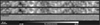 |
Fig. 2 Deflection field (x component) from a simulation of ψDM with λ = 10 pc. The top panel shows the original simulated deflection field. The middle panel illustrates the Gaussian decomposition of this field at 50 times the resolution and obtained with 500 Gaussian functions. The bottom panel represents the difference, which is at the percent level. We used the Gaussian decomposition to interpolate the deflection field to much higher resolutions. The Gaussian decomposition for the y component of the deflection field looks similar. |
4 Magnification of ψDM in the image plane
The magnification in the image plane is not always representative of the observed magnification, especially for ψDM models, since in this case a source typically forms multiple images (usually separated by distances comparable to λdB), all of them very close to each other and appearing in astronomical images as a single unresolved source. The observed flux is then the sum of all the fluxes from the multiple counterimages. Similarly, the observed magnification corresponds to the sum of all magnifications from the multiple images, which is better estimated in the source plane, not the image plane, as the source plane gives the total magnification of all images produced in the image plane. However, it is still instructive to study the properties of the magnification in the image plane, because some properties of the lensed sources can only be measured in the image plane and depend on the DM model. One such property is the clustering of the observed images, since these can form around the projected ψDM constructive (or destructive) interference, hence revealing the scale and mass of the ALP.
In Fig. 3, we show the magnification (on a log scale) for a ψDM model with λ = 10 pc and in different portions of the image plane at different distances d from the CC, where the macromodel magnification takes different values (μ = μtμr ∝ d−1 and as indicated in the top left of each panel). For the sake of simplicity, we assumed the radial component of the magnification was the same in all cases (μr = 1.6). This was well motivated since near the CC, only the tangential component of the macromodel magnification changes rapidly. All regions shown in the figure are in a portion of the lens plane where images have positive parity. The CCs look very similar for the region on the opposite side of the CC and with negative parity.
From top to bottom, we see how small ψDM CCs form near the peaks of the ψDM projected field. At relatively small macro-model magnification factors, the CCs are not connected, but as we increase the macromodel magnification, the ψDM CCs grow in size and start merging with neighboring ψDM CCs. At macro-model magnification factors of μ = 80, the ψDM CCs almost fill the available space. At the highest macromodel magnification we consider, μ = 1600, the ψDM CCs have already formed a corrugated network of ψDM CCs.
The appearance of the ψDM CCs and the corrugated network is very similar when computed assuming the macromodel magnification is negative (or on the side where macroimages have negative parity). However, in this case ψDM CCs tend to form on the complementary space where ψDM forms pockets of small magnification in Fig. 3. An example is illustrated in Fig. 4, where we show the magnification in both scenarios of positive and negative parities, for the same ψDM fluctuation. The white lines correspond to the same ψDM CCs in the yellow square in Fig. 3 (positive parity), while the black curve represents the ψDM CCs that formed around the same region but when we changed the macromodel magnification from μ = 16 to μ = −16. This effect was already noted by Amruth et al. (2023), who describe how when the parity is positive, ψDM CCs form around the positive fluctuations, whereas when the parity is negative, ψDM CCs form around the negative fluctuations. In this sense, the morphology of ψDM CCs is different from the CCs predicted by microlenses or millilenses, that form a well defined hourglass shape, but which is oriented differently depending on whether the parity of the macromodel is positive or negative (Chang & Refsdal 1979).
The probability of magnification computed in the image plane and for both parities is shown in Fig. 5. This probability was simply computed by counting pixels in Fig. 3 that fall within a given magnification interval (in lo units). Dotted lines indicate the relative probability of magnification (computed in logarithmic bins) for regions with varying macromodel magnification on the side with positive parity. Dashed lines show the case for the same regions but with negative parity. Different colors are used to distinguish different macromodel values. These colors, together with the corresponding macromodel value, are given in the bottom of the figure as vertical solid line markers. The positions of these markers indicate the macromodel magnification for each particular region. For ψDM on cluster lenses, there seems to be no distinction between the sides with positive or negative parity (but see Amruth et al. 2023, for galaxy-scale lenses where the situation is different), making it a distinctive feature of this model when compared to CDM plus substructure (CDM+substructure) predictions (Diego et al. 2018; Williams et al. 2024). The probability of magnification in the image plane is very similar for macromodel magnification factors of μ ≳ 100. This would correspond to the saturation regime described by Diego et al. (2018) for the case of microlensing near CCs, but in this case applied to ψDM, where, from Fig. 3 we can see how the corrugated network has already formed for μ ≈ 100.
In all cases, the tail of the distribution follows the canonical dN/dμ ∝ μ−2, or dN/dlog(μ) ∝ μ−1, as in CDM. The probability of magnification shown in Fig. 5 does not include the effect of microlenses or millilenses, but these are known to only slightly modify the probability of magnification when considering large areas ![Mathematical equation: $\[\left(A \gg \lambda_{\mathrm{dB}}^2\right)\]$](/articles/aa/full_html/2024/10/aa51246-24/aa51246-24-eq4.png) in the image plane (Diego et al. 2018; Williams et al. 2024). On the other hand, on smaller scales, comparable to λdB, microlenses or millilenses are expected to significantly modify the probability of magnification, disrupting the ψDM CCs and redistributing the magnification by lowering the magnification at the ψDM CC positions and increasing it around microlenses and millilenses. A detailed study of this effect on very small scales is beyond the scope of this paper and will be treated in a future work.
in the image plane (Diego et al. 2018; Williams et al. 2024). On the other hand, on smaller scales, comparable to λdB, microlenses or millilenses are expected to significantly modify the probability of magnification, disrupting the ψDM CCs and redistributing the magnification by lowering the magnification at the ψDM CC positions and increasing it around microlenses and millilenses. A detailed study of this effect on very small scales is beyond the scope of this paper and will be treated in a future work.
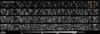 |
Fig. 3 Magnification in the image plane for a ψDM model with a de Broglie wavelength of 10 pc and in regions with positive parity. The top panel shows the ψDM CC (magnification in gray scale) formed by ψDM with λ = 10 pc in a region with macromodel magnification μ = 10 × 1.6 = 16 and positive parity. The bottom panels show the same realization of ψDM but for increasing values of the tangential macromodel magnification (in the horizontal direction) or, similarly, for smaller distances to the macromodel CC, while the radial component (vertical direction) is maintained at μr = 1.6. The macromodel magnification, μ, typically scales with the distance, d, to the macromodel CC as μ ∝ 1/d. In this configuration, and in the absence of ψDM fluctuations or small-scale perturbations in the deflection field, the cluster CC would appear as a single vertical line when d = 0 or μt = ∝. The scale is the same in all plots. The corresponding distribution of magnification values is shown in Fig. 5. The yellow square in the top panel indicates the region shown in Fig. 4. |
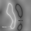 |
Fig. 4 Dependence of CCs on parity. The image shows the sum of the logarithm of magnifications (gray scale), log(μ+) − log(μ−), from the same ψDM perturbation but for the two parities, μ+ and μ−. For this particular case, the ψDM perturbation contained both positive and negative fluctuations in mass and corresponds to the yellow square region in the top panel of Fig. 3. The white line represents the ψDM CC when the ψDM perturbation is on the side with positive parity (as in Fig. 3). The black line represents the ψDM CC when the same ψDM perturbation is on the side with negative parity. |
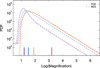 |
Fig. 5 Probability of magnification for ψDM in the image plane. The probability was derived from the regions shown in Fig. 3 by counting the area (or pixels) with a given magnification. Each color corresponds to a different macromodel magnification, indicated by the thick vertical solid lines. The dotted and dashed lines correspond to the positive (POS) and negative (NEG) macromodel magnifications, respectively. The probability of magnification in the image plane is not representative of the observed magnification since it does not account for the multiplicity of images. |
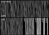 |
Fig. 6 Caustics for ψDM. The top panel shows the caustics (magnification in gray scale) formed by ψDM with λ = 10 pc in a region with macromodel magnification μ = 10 × 1.6 = 16 and positive parity, that is, 80 × 31.2 pc2 in the source plane. The bottom panel displays the same realization of ψDM but with increasing values of the tangential macromodel magnification (and hence, smaller areas in the source plane) while the radial component is maintained at μr = 1.6. The cluster caustic is not shown but would be a thin vertical line to the right of the bottom-right panel. The scale is the same in all plots. The caustics with the same macromodel magnification but negative parity look almost indistinguishable. The corresponding distributions of magnification values are shown in Fig. 7. |
5 Magnification of ψDM in the source plane
The true magnification experienced by a small source moving across the web of ψDM caustics is the one computed in the source plane. We computed the magnification in the source plane using standard ray tracing and for the same regions with varying macromodel magnification discussed in the previous section.
The resulting magnification pattern in the source plane is displayed in Fig. 6. This image represents the best view of the ψDM caustics to date. The top panel shows the region with the smallest macromodel magnification, μ = 16. The bottom row illustrates the remaining regions with increasing macromodel magnification values (shown in or near the top-left corner of each panel). The cluster CC is not shown, but in our configuration it would appear as a vertical white line at the right edge of the bottom panel. This figure shows only the case of positive parity; the negative-parity case looks very similar and hence is not displayed here.
One striking difference between the ψDM and CDM substructures (microlenses and millilenses) is that in the case of ψDM, the magnification pattern is nearly identical, independent of the parity. This was already demonstrated by the toy model discussed in Sec. 2. This similarity is better demonstrated in Fig. 7, where we show the distribution of magnification in the source plane for regions with different parity and different macromodel magnification values. The line and color scheme is similar to that in Fig. 5.
This is not the case in classic CDM simulations where substructure is composed of either point sources (microlenses) or cuspy halos (millilenses). These halos correspond to dwarf galaxies, globular clusters, ultracompact dwarf galaxies, or DM halos in general. One common characteristic of the microlenses and millilenses studied in the context of CDM is that when they are found in regions of negative parity they can significantly demagnify sources below the macromodel value, while on the side with positive parity only very modest demagnification can take place. In CDM, significant demagnification on the side with positive parity would be possible only with objects having negative mass. These hypothetical objects behave as similar objects but with positive mass on the side with negative parity. In ψDM, negative-mass objects are equivalent to the negative δρ/ρ ≪ 1 fluctuations which can naturally demagnify distant objects aligned behind them.
In the ψDM scenario, demagnification can take place for both parities, and with similar probability independent of the parity. On the other hand, similar to the CDM+substructure case, the maximum variance in the magnification takes place in situations where the saturation regime is reached, which in our case was for macromodel magnification μ ≈ 100.
For the cases with macromodel magnification μ < 100, the tail of the distribution in Fig. 7 falls faster than the expected dN/dlog(μ) ∝ μ−2, but this is partially an artifact due to the limited size of the pixel in the simulation. We do expect the dN/dlog(μ) ∝ μ−2 tail to extend to higher magnifications, but not to infinity because at some point microlenses near the ψDM caustics (and not included in our simulation) will transform the μ−2 power law into log normal, as described by Diego et al. (2018, 2020) and Palencia et al. (2024). For large macromodel values μ≫ 100, we observed the log-normal distribution predicted also for the case of microlenses near CCs. In addition, a finite-pixel effect is expected here for the largest magnification factors, but combined with the faster decline from the log-normal behavior due to the combined effect of overlapping ψDM caustics. Adding microlenses to the ψDM model in the regime where the macromodel magnification is already μ ≫ 100 should have little impact on the log-normal distribution of magnifications, since the log-normal shape (and position of the central peak) would be maintained, but the addition of microlenses should broaden it by a small amount. A similar argument can be made for the addition of millilenses, except in this case we expect a modification of the probability of magnification near the millilens that can imprint a distortion in the deflection field on a scale similar to the de Broglie wavelength. We leave the detailed study of ψDM plus millilenses and microlenses for future work. The case of microlenses plus millilenses was studied (in the context of CDM) by Diego et al. (2024).
If we look at the maxima of all the probabilities in Fig. 5, we observe how these maxima scale as 1/μ, departing from the expected 1/μ2 of the macromodel (when taking logarithmic bins in the magnification, as done in this figure). This is because the area in the image plane is the same for all curves, but in a real-world scenario, the curves with lower macromodel magnification would originate from regions with a correspondingly larger area, so this envelope should be corrected by an additional factor μ−1 and hence recovering the expected μ−2 scaling of the macro-model. In other words, as in the case of substructure in CDM, ψDM does not modify the overall probability of magnification on scales larger than the de Broglie scale. Instead, the magnification (or flux) is simply redistributed, with ψDM fluctuations far away from the cluster CC borrowing high magnification values from the CC. This mechanism is similar in CDM+substructure.
As in CDM, we do expect the maximum magnification of a small object (for instance a star) in the corrugated network to be significantly less than in the case of smooth CDM. This reduction in maximum magnification is due to the small-scale perturbations in the deflection field, which increase the curvature of the deflection field on small scales. Since the maximum magnification when crossing a caustic is inversely proportional to this curvature (Schneider et al. 1992), ψDM fluctuations near the cluster CC also decrease the maximum magnification of a star when crossing a ψDM caustic. The amount of this reduction is expected to scale inversely proportional to λdB, since smaller λdB results in higher local curvature. The exact scaling of the maximum magnification with λdB is also beyond the scope of this paper and will be treated in future work.
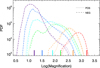 |
Fig. 7 Probability of magnification for ψDM in the source plane. The probability is derived from the regions shown in Fig. 6. Each color corresponds to a different macromodel magnification, indicated by the thick vertical solid lines. The dotted and dashed lines correspond to the positive and negative macromodel magnifications, respectively. |
6 Discussion
Perhaps the most interesting feature of the curves shown in Fig. 7 is the fact that ψDM perturbations on the side with positive parity have the capacity to demagnify (with respect to the macro-model value). Next, we discuss how this is not possible with substructures in CDM (such as millilenses or microlenses). To better show this difference, we compared the expected probability of magnification in CDM+substructure with the ψDM case. We did this by adding microlenses to a smooth CDM model, since microlenses, similarly to ψDM fluctuations, are ubiquitous in the image plane. Millilenses, on the other hand, although producing deflection fields with similar amplitude as ψDM, are much rarer in the image plane, so the probability of magnification depends on whether it is computed near to, or far from, a millilens.
We considered the particular case of macromodel magnification μmacro = 80 (light-blue curves in Fig. 7) for which a prominent demagnification (i.e., μ < 80) peak forms around μ = 20. This value of μmacro corresponds to the threshold where the corrugated network of ψDM caustics starts to form and magnification distortions are greatest. For the microlenses, we considered a case with surface mass density of microlenses ∑* ≈ 20 M⊙ pc−2. This is a value typically found near CCs, where stellar microlenses from the intracluster medium contribute ~1% to the total projected mass, and this is typically ∑Tot = κ × ∑crit ≈ 2000 M⊙ pc−2 (for convergence values κ ≈ 0.6, as usually found near cluster CCs). We computed the probability of magnification in the CDM plus microlenses (CDM+microlenses) case with the microlensing code from Palencia et al. (2024), adopting the parameters described above. The resulting probability of magnification in both cases, ψDM and CDM+microlenses, is shown in Fig. 8. The probability of magnification for ψDM is indicated as dark-blue curves (the same curves are light blue in Fig. 7). The curves for CDM+microlenses are shown as red curves. When comparing the two curves with positive parity, at low magnification values μ ≈ 20, ψDM (dotted blue) has orders of magnitude more probability of demagnifying (that is, values of μ < 80) than the CDM+microlenses case (dotted red). Increasing the amount of microlenses would result in a curve that is slightly wider but not enough to significantly increase the probability of relative demagnification.
Adding microlenses to ψDM does not change this conclusion. Microlenses would widen the dark-blue dotted line as if convolved by the red dotted line, still leaving a prominent peak at μ ≈ 20, which cannot be reproduced by CDM+substructure (even millilenses). Demagnification of images by more than a factor of ~2 is only possible on the side with positive parity for ψDM. This demagnification is not only possible in ψDM but highly likely at the boundaries of the corrugated network. On the side with negative parity, similar high magnification factors and probabilities are expected in ψDM and CDM+substructure. In contrast, demagnification is less pronounced in the case of ψDM than in the case of CDM+substructure, so demagnification factors greater than one order of magnitude are much less likely in ψDM, while they are still quite likely in CDM+substructure.
When confronting these predictions with observations, a good example to consider is the Lyman continuum (LyC) knot in the Sunburst arc (Rivera-Thorsen et al. 2019), where up to 12 highly magnified images of the same compact structure are seen multiply lensed. This LyC knot is large enough to be insensitive to microlensing, but small enough that it can be affected by ψDM perturbations. Other small structures in the arc are also observed multiple times, with some of them (such as the alleged lensed star Godzilla) presenting highly anomalous magnifications (Diego et al. 2022).
These authors suggested that Godzilla can be explained in the context of the standard CDM and claimed that an undetected dwarf-galaxy millilens was responsible for its anomalous magnification. The alleged millilens was later discovered in deeper JWST data by Choe et al. (2024). While CDM may be the right explanation at this point, if more Godzilla-like objects are detected, CDM may become disfavored because the amount of substructure needed (or its ubiquity) may be inconsistent with the CDM scenario and better explained by ψDM, where lensing perturbations are expected to be affecting all images in the Sunburst arc. The very clear and fundamental differences in how images with different parities can be demagnified can be used to discriminate between CDM and ψDM with current observations and detailed lens models of arcs such as the Sunburst arc.
Another interesting object is the Dragon arc in Abell 370, where Fudamoto et al. (2024) report over 40 alleged microlensing events. Most of these events are found on the side of the CC with negative parity, as shown by Broadhurst et al. (2024). This is consistent with the findings in this paper: before adding microlenses, the probability of magnification is similar on both sides of the CC, but when microlenses are added, images with negative parity are more likely to be detected since they carry larger magnifications near the CCs than their counterimages with positive parity, as a consequence of the demagnification between caustics produced by microlenses (in negative parity region), which needs to be compensated with higher magnification factors near the caustics in order to maintain the mean magnification invariant. We leave the detailed interpretation of these events in the context of ψDM for a future paper, after the macromodel around the Dragon arc has been updated with the new constraints from the recent JWST observations.
An additional way of distinguishing between CDM and ψDM is based on the scale of the background source. As we have seen, both ψDM and microlenses produce ubiquitous fluctuations in the deflection field, although they result in different probabilities of demagnification. Very small but luminous objects, such as supergiant stars, can be very effectively magnified and demagnified by microlenses. The size of microcaustics from stars in the intracluster medium is typically 10−3 pc, so objects 1 pc in size become immune to microlensing distortions and can be magnified or demagnified only by more massive structures in CDM, such as millilenses. At 1 pc, ψDM is still very efficient at magnifying and demagnifying, and at ~0.5 pc the efficiency is maximum for de Broglie wavelengths λ ≈ 10 pc (see Fig. 7). A high occurrence of demagnification of parsec-scale structures would be inconsistent with CDM since the number density of millilenses in the image plane is not very high, while ψDM fluctuations are always taking place in the image plane and thus the probability of demagnification is always ~50%.
Recent observations with JWST have revealed the existence of very small but bright star clusters at high redshift (Vanzella et al. 2023; Adamo et al. 2024), corroborating the highly compact nature of some of these luminous objects in local measurements (Brown & Gnedin 2021). Compact stellar clusters make perfect candidates for mapping DM substructure in the lens plane on subparsec scales, and in particular for testing ψDM models. These objects are big enough that they should be almost insensitive to microlensing distortions, but sufficiently small to be smaller than the demagnification region in the source plane produced by ψDM fluctuations. At the same time, these small clusters are bright enough to still be observed with demagnification factors of 4–5, relative to the macromodel value, when μmacro ≈ 100, which is the range of macromodel magnifications where we expect ψDM lensing distortions to be maximum. The spatial distribution of JWST microlenses in critically lensed galaxies recently uncovered by Fudamoto et al. (2024) and Yan et al. (2023) can help discriminate between these possibilities. Most of the new microlensing events are found in a broad band around the CC, with a tendency toward negative parity. This is consistent with the ψDM scenario once the extra magnification from microlenses, in addition to the boost in magnification provided by ψDM fluctuations, is taken into account (see Broadhurst et al. 2024, for details).
So far, the conclusions derived in this work were obtained for a ψDM model with λdB = 10 pc. The properties of magnification should depend on the de Broglie wavelength, as indicated by earlier work (Amruth et al. 2023). A detailed study of the dependence of our conclusions on λdB is beyond the scope of this paper, but from earlier work we can conclude that the width of the corrugated network grows as ![Mathematical equation: $\[\lambda_{\mathrm{dB}}^{0.5}\]$](/articles/aa/full_html/2024/10/aa51246-24/aa51246-24-eq5.png) , and in the limit of the high boson mass (very small λdB), one should recover the smoothlens case with no corrugated network. It is expected that, as in the case of microlenses, the probability of magnification in ψDM can be entirely described by an effective surface mass density of ψDM perturbations, ∑eff = ∑dB(λdB) × μmacro, where ∑dB(λdB) is some function of λdB of the form
, and in the limit of the high boson mass (very small λdB), one should recover the smoothlens case with no corrugated network. It is expected that, as in the case of microlenses, the probability of magnification in ψDM can be entirely described by an effective surface mass density of ψDM perturbations, ∑eff = ∑dB(λdB) × μmacro, where ∑dB(λdB) is some function of λdB of the form ![Mathematical equation: $\[\Sigma_{\mathrm{dB}}\left(\lambda_{\mathrm{dB}}\right) \propto \lambda_{\mathrm{dB}}^\alpha\]$](/articles/aa/full_html/2024/10/aa51246-24/aa51246-24-eq6.png) with α > 0 (see Broadhurst et al. 2024, for further details).
with α > 0 (see Broadhurst et al. 2024, for further details).
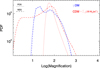 |
Fig. 8 Comparison of magnification with ψDM and CDM+microlenses. Dotted lines represent regions having positive parity while dashed lines are for negative parity. In all curves, the macromodel magnification is set to 80. In the case of CDM (red curves), the substructure is created by microlenses with surface mass density 20 M⊙ pc−2. The addition of microlenses to ψDM would slightly broaden the dashed-line curves, but maintaining the demagnification peak (that is, at μ < 80) on the side with positive parity. |
7 Conclusions
We have generated the first high-resolution images of the source plane in a model of ψDM with λ = 10 pc and in regions very close to the CC of a galaxy cluster lens. The perturbations in ψDM result in pockets of low magnification in the source plane with scales of ~0.5 pc. These low-magnification regions are typical in CDM+substructure scenarios for images with negative parity, but we find that in the case of ψDM they also appear on the side of the CC with positive parity. Demagnification of parsec-scale objects in their positive-parity counterimages cannot be reproduced by substructure in CDM, but are likely in ψDM, making this a unique testable feature of ψDM models.
Images with positive and negative parity have very similar distributions of magnification. This differs distinctly from CDM predictions, where the positive- and negative-parity images are clearly distinguishable, especially for macromodel images with μmacro < 100. In particular, ψDM alone cannot demagnify negative-parity images as much as CDM substructure. Adding microlenses to ψDM increases the probability of demagnification for images with negative parity, bringing the results close to CDM predictions, but does not significantly enhance the demagnification of images with positive parity. This behavior is unique to ψDM. Current and future observations of multiple images from parsec-scale star clusters near cluster CCs can be used to further test ψDM models.
Acknowledgements
We thank the anonymous referee for useful comments and feedback. J.M.D. acknowledges support from project PID2022-138896NB-C51 (MCIU/AEI/MINECO/FEDER, UE) Ministerio de Ciencia, Investigación y Universidades. J.L., S.K.L., and A.A. are funded by grants RGC/GRF 17312122 and RGC/CRF C6017-20G. R.A.W. acknowledges NASA JWST Interdisciplinary Scientist grants NAG5-12460, NNX14AN10G, and 80NSSC18K0200 from GSFC. A.V.F. received financial assistance from the Christopher R. Redlich Fund and many individual donors. L.L.R.W. acknowledges the support of HST SNAP program GO-17504.
References
- Abbott, T. M. C., Aguena, M., Alarcon, A., et al. 2022, Phys. Rev. D, 105, 023520 [CrossRef] [Google Scholar]
- Adamo, A., Bradley, L. D., Vanzella, E., et al. 2024, arXiv e-prints [arXiv:2401.03224] [Google Scholar]
- Alam, S., Aubert, M., Avila, S., et al. 2021, Phys. Rev. D, 103, 083533 [NASA ADS] [CrossRef] [Google Scholar]
- Amruth, A., Broadhurst, T., Lim, J., et al. 2023, Nat. Astron., 7, 736 [NASA ADS] [CrossRef] [Google Scholar]
- Broadhurst, T., Li, S. K., Alfred, A., et al. 2024, arXiv e-prints [arXiv:2405.19422] [Google Scholar]
- Brown, G., & Gnedin, O. Y. 2021, MNRAS, 508, 5935 [NASA ADS] [CrossRef] [Google Scholar]
- Chan, J. H. H., Schive, H.-Y., Wong, S.-K., Chiueh, T., & Broadhurst, T. 2020, Phys. Rev. Lett., 125, 111102 [NASA ADS] [CrossRef] [Google Scholar]
- Chang, K., & Refsdal, S. 1979, Nature, 282, 561 [Google Scholar]
- Choe, S., Rivera-Thorsen, T. E., Dahle, H., et al. 2024, A&A, submitted https://arxiv.org/pdf/2405.06953 [NASA ADS] [CrossRef] [EDP Sciences] [Google Scholar]
- DESI Collaboration (Adame, A. G., et al.) 2024, arXiv e-prints [arXiv:2404.03002] [Google Scholar]
- Diego, J. M., Kaiser, N., Broadhurst, T., et al. 2018, ApJ, 857, 25 [NASA ADS] [CrossRef] [Google Scholar]
- Diego, J. M., Molnar, S. M., Cerny, C., et al. 2020, ApJ, 904, 106 [NASA ADS] [CrossRef] [Google Scholar]
- Diego, J. M., Pascale, M., Kavanagh, B. J., et al. 2022, A&A, 665, A134 [NASA ADS] [CrossRef] [EDP Sciences] [Google Scholar]
- Diego, J. M., Li, S. K., Amruth, A., et al. 2024, A&A, 689, A167 [NASA ADS] [CrossRef] [EDP Sciences] [Google Scholar]
- Enzi, W., Murgia, R., Newton, O., et al. 2021, MNRAS, 506, 5848 [NASA ADS] [CrossRef] [Google Scholar]
- Fudamoto, Y., Sun, F., Diego, J. M., et al. 2024, arXiv e-prints [arXiv:2404.08045] [Google Scholar]
- Gilman, D., Bovy, J., Treu, T., et al. 2021, MNRAS, 507, 2432 [NASA ADS] [CrossRef] [Google Scholar]
- Hu, W., Barkana, R., & Gruzinov, A. 2000, Phys. Rev. Lett., 85, 1158 [NASA ADS] [CrossRef] [Google Scholar]
- Hui, L. 2021, ArA&A, 59, 247 [NASA ADS] [CrossRef] [Google Scholar]
- Laroche, A., Gilman, D., Li, X., Bovy, J., & Du, X. 2022, MNRAS, 517, 1867 [NASA ADS] [CrossRef] [Google Scholar]
- Liu, J., Gao, Z., Biesiada, M., & Liao, K. 2024, arXiv e-prints [arXiv:2405.04779] [Google Scholar]
- Messa, M., Dessauges-Zavadsky, M., Adamo, A., Richard, J., & Claeyssens, A. 2024, MNRAS, 529, 2162 [CrossRef] [Google Scholar]
- Navarro, J. F., Frenk, C. S., & White, S. D. M. 1996, ApJ, 462, 563 [Google Scholar]
- Palencia, J. M., Diego, J. M., Kavanagh, B. J., & Martínez-Arrizabalaga, J. 2024, A&A, 687, A81 [Google Scholar]
- Peebles, P. J. E. 2000, ApJ, 534, L127 [NASA ADS] [CrossRef] [Google Scholar]
- Planck Collaboration XIII. 2016, A&A, 594, A13 [NASA ADS] [CrossRef] [EDP Sciences] [Google Scholar]
- Planck Collaboration VI. 2020, A&A, 641, A6 [NASA ADS] [CrossRef] [EDP Sciences] [Google Scholar]
- Powell, D. M., Vegetti, S., McKean, J. P., et al. 2023, MNRAS, 524, L84 [NASA ADS] [CrossRef] [Google Scholar]
- Press, W. H., Ryden, B. S., & Spergel, D. N. 1990, Phys. Rev. Lett., 64, 1084 [NASA ADS] [CrossRef] [Google Scholar]
- Ragagnin, A., Meneghetti, M., Calura, F., et al. 2024, A&A, 687, A270 [NASA ADS] [CrossRef] [EDP Sciences] [Google Scholar]
- Rivera-Thorsen, T. E., Dahle, H., Chisholm, J., et al. 2019, Science, 366, 738 [Google Scholar]
- Schive, H.-Y., Chiueh, T., & Broadhurst, T. 2014, Nat. Phys., 10, 496 [NASA ADS] [CrossRef] [Google Scholar]
- Schive, H.-Y., Chiueh, T., Broadhurst, T., & Huang, K.-W. 2016, ApJ, 818, 89 [NASA ADS] [CrossRef] [Google Scholar]
- Schneider, P., Ehlers, J., & Falco, E. E. 1992, Gravitational Lenses (Berlin: Springer) [Google Scholar]
- Vanzella, E., Claeyssens, A., Welch, B., et al. 2023, ApJ, 945, 53 [NASA ADS] [CrossRef] [Google Scholar]
- Weinberg, D. H., Bullock, J. S., Governato, F., Kuzio de Naray, R., & Peter, A. H. G. 2015, Proc. Natl. Acad. Sci., 112, 12249 [NASA ADS] [CrossRef] [Google Scholar]
- Widrow, L. M., & Kaiser, N. 1993, ApJ, 416, L71 [NASA ADS] [CrossRef] [Google Scholar]
- Williams, L. L. R., Kelly, P. L., Treu, T., et al. 2024, ApJ, 961, 200 [NASA ADS] [CrossRef] [Google Scholar]
- Yan, H., Ma, Z., Sun, B., et al. 2023, ApJS, 269, 43 [NASA ADS] [CrossRef] [Google Scholar]
In CDM, positive perturbations in mass in regions of the lens plane with negative parity are equivalent to negative perturbations in mass in the symmetric regions with positive parity.
All Figures
|
Fig. 1 Caustics for a toy model of an individual and isolated ψDM perturbation. For this example, the ψDM fluctuation is positive. The left and right panels show the caustics produced by the same 2 pc-scale ψDM fluctuation, but on the two sides of the lens CC and at the same distance. That is, they represent the fluctuation in the positive- and negative-parity sides with the same macromodel magnification. In both cases, the macromodel magnification is 160. The caustics are almost indistinguishable, with just a small shift in position. The white dot marks the same position in the source plane, so the shift of the caustics with respect to this point indicates the shift in position when we vary the parity. A negative fluctuation in the deflection field of ψDM (not shown) results in similar caustics, but which are mirrored in the horizontal direction. |
| In the text | |
|
Fig. 2 Deflection field (x component) from a simulation of ψDM with λ = 10 pc. The top panel shows the original simulated deflection field. The middle panel illustrates the Gaussian decomposition of this field at 50 times the resolution and obtained with 500 Gaussian functions. The bottom panel represents the difference, which is at the percent level. We used the Gaussian decomposition to interpolate the deflection field to much higher resolutions. The Gaussian decomposition for the y component of the deflection field looks similar. |
| In the text | |
|
Fig. 3 Magnification in the image plane for a ψDM model with a de Broglie wavelength of 10 pc and in regions with positive parity. The top panel shows the ψDM CC (magnification in gray scale) formed by ψDM with λ = 10 pc in a region with macromodel magnification μ = 10 × 1.6 = 16 and positive parity. The bottom panels show the same realization of ψDM but for increasing values of the tangential macromodel magnification (in the horizontal direction) or, similarly, for smaller distances to the macromodel CC, while the radial component (vertical direction) is maintained at μr = 1.6. The macromodel magnification, μ, typically scales with the distance, d, to the macromodel CC as μ ∝ 1/d. In this configuration, and in the absence of ψDM fluctuations or small-scale perturbations in the deflection field, the cluster CC would appear as a single vertical line when d = 0 or μt = ∝. The scale is the same in all plots. The corresponding distribution of magnification values is shown in Fig. 5. The yellow square in the top panel indicates the region shown in Fig. 4. |
| In the text | |
|
Fig. 4 Dependence of CCs on parity. The image shows the sum of the logarithm of magnifications (gray scale), log(μ+) − log(μ−), from the same ψDM perturbation but for the two parities, μ+ and μ−. For this particular case, the ψDM perturbation contained both positive and negative fluctuations in mass and corresponds to the yellow square region in the top panel of Fig. 3. The white line represents the ψDM CC when the ψDM perturbation is on the side with positive parity (as in Fig. 3). The black line represents the ψDM CC when the same ψDM perturbation is on the side with negative parity. |
| In the text | |
|
Fig. 5 Probability of magnification for ψDM in the image plane. The probability was derived from the regions shown in Fig. 3 by counting the area (or pixels) with a given magnification. Each color corresponds to a different macromodel magnification, indicated by the thick vertical solid lines. The dotted and dashed lines correspond to the positive (POS) and negative (NEG) macromodel magnifications, respectively. The probability of magnification in the image plane is not representative of the observed magnification since it does not account for the multiplicity of images. |
| In the text | |
|
Fig. 6 Caustics for ψDM. The top panel shows the caustics (magnification in gray scale) formed by ψDM with λ = 10 pc in a region with macromodel magnification μ = 10 × 1.6 = 16 and positive parity, that is, 80 × 31.2 pc2 in the source plane. The bottom panel displays the same realization of ψDM but with increasing values of the tangential macromodel magnification (and hence, smaller areas in the source plane) while the radial component is maintained at μr = 1.6. The cluster caustic is not shown but would be a thin vertical line to the right of the bottom-right panel. The scale is the same in all plots. The caustics with the same macromodel magnification but negative parity look almost indistinguishable. The corresponding distributions of magnification values are shown in Fig. 7. |
| In the text | |
|
Fig. 7 Probability of magnification for ψDM in the source plane. The probability is derived from the regions shown in Fig. 6. Each color corresponds to a different macromodel magnification, indicated by the thick vertical solid lines. The dotted and dashed lines correspond to the positive and negative macromodel magnifications, respectively. |
| In the text | |
|
Fig. 8 Comparison of magnification with ψDM and CDM+microlenses. Dotted lines represent regions having positive parity while dashed lines are for negative parity. In all curves, the macromodel magnification is set to 80. In the case of CDM (red curves), the substructure is created by microlenses with surface mass density 20 M⊙ pc−2. The addition of microlenses to ψDM would slightly broaden the dashed-line curves, but maintaining the demagnification peak (that is, at μ < 80) on the side with positive parity. |
| In the text | |
Current usage metrics show cumulative count of Article Views (full-text article views including HTML views, PDF and ePub downloads, according to the available data) and Abstracts Views on Vision4Press platform.
Data correspond to usage on the plateform after 2015. The current usage metrics is available 48-96 hours after online publication and is updated daily on week days.
Initial download of the metrics may take a while.