| Issue |
A&A
Volume 665, September 2022
|
|
|---|---|---|
| Article Number | A127 | |
| Number of page(s) | 7 | |
| Section | Numerical methods and codes | |
| DOI | https://doi.org/10.1051/0004-6361/202244027 | |
| Published online | 23 September 2022 | |
Fast algorithm for simulating light curves of stars at extreme magnification affected by microlensing
Instituto de Física de Cantabria (CSIC-UC),
Avda. Los Castros s/n,
39005
Santander, Spain
e-mail: This email address is being protected from spambots. You need JavaScript enabled to view it.
Received:
15
May
2022
Accepted:
9
July
2022
Abstract
We present a fast algorithm aimed at reproducing the light curves of distant stars undergoing microlensing near critical curves. The need for these type of algorithms has been motivated by recent observations of microlensing events of distant stars at high redshift and involving extreme magnification factors. The algorithm relies on a low-resolution computation of the deflection field due to an ensemble of microlenses near critical curves and takes advantage of the gradually varying nature of the deflection field to infer the magnification of the unresolved images. The algorithm is capable of resolving microlenses at cosmological distances with planet-sized masses, as well as typical background luminous stars of a few solar radii. Using this algorithm, light curves covering decades of relative motion between the source and the web of microcaustics, at nanoarcsec resolution, can be reproduced within a matter of minutes on a basic laptop. Classic inverse ray tracing simulations at the same resolution would take days or weeks to produce, consuming massive computational resources.
Key words: gravitational lensing: strong / methods: numerical
© J. M. Diego 2022
 Open Access article, published by EDP Sciences, under the terms of the Creative Commons Attribution License (https://creativecommons.org/licenses/by/4.0), which permits unrestricted use, distribution, and reproduction in any medium, provided the original work is properly cited.
This article is published in open access under the Subscribe-to-Open model. This email address is being protected from spambots. You need JavaScript enabled to view it. to support open access publication.
1 Introduction
The observation of Icarus in 2018 (Kelly et al. 2018) by the Hubble Space Telescope (HST) represents the advent of a new branch of astrophysics: the study of individual stars at cosmo-logical distances. Icarus, at z = 1.49 behind the MACS J1149 cluster, was the first individual star ever observed beyond red-shift z = 1 and challenged the record of the farthest individual observed star by a factor of ≈200 in terms of comoving distance, with the previous record holder (SDSS J1229+1122, Ohyama & Hota 2013) located in the nearby Virgo cluster and less than 20 Mpc away. Icarus was detected thanks to the combined effect of a large macromodel magnification factor (µ ≈ 500), plus the boost contributed by a microlens, momentarily intersecting the path of the photons (adding an extra factor µ ≈ 4 to the total magnification), resulting in a net magnification factor of µ ≈ 2000. At magnification factors of µ = 2000, there is a net gain of more than eight magnitudes, making stars that would otherwise go undetected with current technology bright enough to be detected by telescopes such as HST. This technique allows us to reach a vast volume beyond redshift z = 1 comprising thousands of Gpc3 (between z ~ 1 and z ~ 10). This volume is millions of times larger than the volume accessible in our local universe without the aid of lensing (roughly up to 20 Mpc), and where we have been so far limited to study a relatively small number of very bright stars. Given the low probability of lensing, only a very small fraction of the stars at z > 1 are capable of being detected by our telescopes, but the large volume at z > 1 sufficiently compensates for the low probability of lensing, making the number of detectable stars at cosmic distances no-negligible. The specific number of detectable stars at cosmic distances depends on the abundance of luminous stars, which, in turns, depends on the poorly constrained mass function of stars at high redshift. A census of strongly lensed stars at cosmic distances can then be used to infer the high end of the mass function of stars. Stars undergoing microlensing events can be identified by algorithms designed to search for transients such as supernovae (SNe). Other stars that are being strongly magnified near critical curves have been identified in recent years. Behind the MACS J0416 galaxy cluster, several candidate strongly lensed stars have been identified (Rodney et al. 2018; Chen et al. 2019; Kaurov et al. 2019). Among these, there is one candidate in particular, dubbed Warhol at z = 0.94, that has unambiguously been identified as a star (Chen et al. 2019; Kaurov et al. 2019). As in the case of Icarus, Warhol shows temporal variations that are probably due to microlensing. More recently, behind the PSZ1 G311 galaxy cluster, Diego (2019) identified an extremely magnified star, dubbed Godzilla, at a redshift of z = 2.37. As opposed to Icarus and Warhol, Godzilla was not identified due to temporal variations in the flux but due to its unusually bright appearance, lack of counterimages, and unresolved nature. Although it was a previously known object generally (Vanzella et al. 2020), Godzilla was not initially recognized as an extremely lensed star. The high degree of brightness in Godzilla was interpreted by Diego et al. (2022) as due to the star’s being observed during an outburst phase (these outbursts can last decades in the observer frame). Due to its brightness (mAB ≈ 22), Godzilla represents the first star at z > 1 for which a spectrum has been obtained (Vanzella et al. 2020). The MUSE spectrum shows peculiar features also present in massive luminous blue variable stars such as a P-cygni profile (Diego et al. 2022). An interesting fact regarding Godzilla is that no microlensing flux fluctuations have been observed so far. This is consistent with the magnification, µ, from the macro-model is in the range of several thousands. In this situation, as discussed in Diego et al. (2022) and Welch et al. (2022), it is possible to exceed the saturation regime where the effective convergence exceeds 1, that is, κeff > 1. The effective convergence is defined as κeff = κ*µ, where κ* is the dimensionless convergence (i.e., the microlens surface mass density divided by the critical surface mass density), and µ is the macromodel magnification. For typical values of κ* ~ 10−3, the saturation regime is reached when µ ~ 103. Beyond this point, an effect known as the “more-is-less” effect is at work, whereby increasing the magnification results in more overlapping microcaustics in the source plane. Crossing one of these microcaustics results in a relatively small change in flux, since the flux linked to the other microcaustics is still significant and remain more or less constant during the microcaustic crossing. Small flux fluctuations are also expected in the regime of low effective convergence, or κeff ≪ 1, corresponding typically to situations with moderate to small macromodel magnification factors; however, in this case, the flux variability can be distinguished from the previous case since the flux varies slowly with time, while in the case described above, rapid (but small) variations in flux are expected.
The latest example of an extremely magnified star is also the most distant one. Welch et al. (2022) reported the discovery of Earendel, a strongly magnified star at a record breaking redshift z = 6.2, looming at the end of the reionization epoch. Although it is unlikely to be a Pop III star, Earendel represents one of the missing links in the evolution of stellar populations. Earendel was discovered behind the galaxy cluster WHL0137–08 (z = 0.566) in the strongly lensed Sunrise galaxy. This galaxy was first observed in images from the RELICS program (Coe et al. 2019). Although spectral measurements of Earendel are not yet available, and photometric measurements are relatively poor, it is believed that Earendel is a star with very low metallicity and with a high luminosity. Earlier estimates in Welch et al. (2022) would have put Earendel on par with the most luminous stars known in our local universe (R < 40 Mpc). As in the case of Godzilla discussed above, no significant flux variations have been noted during the two epochs (three years apart) in which Earendel was observed. This can be explained by the same “more-is-less” effect since the estimated magnification of Earendel is also in the range of thousands, resulting in multiple overlapping microcautics. However, small flux fluctuations (Δm ≈ 0.5−1 magnitudes) are expected due to microlensing but one needs to wait for deeper observations with the James Webb Space Telescope (JWST)1.
The recently launched JWST arrives at the perfect moment to exploit the recent discovery of extremely magnified distant stars. With its gold-coated mirrors, JWST will lead us to a new golden age in astronomy, exposing previously unknown distant objects with unprecedented detail. Some of these objects will undoubtedly include extremely magnified stars, discovered through the same technique so successfully proven by Hubble. As mentioned earlier, observations of these distant stars represents the beginning of a new branch of astrophysics, where we will learn not only about the physics of the first- and second-generation stars, but also about the small-scale fluctuations in the lens plane that perturb the magnification of the background stars. An interesting aspect of extremely magnified distant stars is that, at large magnification factors, microlensing effects are always present, since the density of microcaustics is scaled as the magnification of the macromodel. The ubiquitous presence of microcaustics in the source plane prohibits magnification factors much greater than a few tens of thousands, even for relatively compact stars with sizes of several solar radii Venumadhav et al. (2017); Diego et al. (2018). In essence, microlenses perturb the lensing potential, thereby increasing its naturally small curvature (when µ is large) around the microlenses. Since the maximum magnification is directly proportional to the inverse of this curvature, microlenses consequently reduce the maximum possible magnification. This is an interesting facet, since it imposes a natural bias toward brighter stars. Without this limitation, it would be difficult to distinguish between the more common stars that are fainter but more magnified and stars that are more luminous but less magnified. A maximum value for the magnification then sets a limit to the lowest possible luminosity of the star at a given redshift. Hence, at extreme magnification factors, JWST will naturally pick up the brightest stars at high redshifts, offering a cleaner view of the massive end of the primeval stellar mass function.
Microlensing events of these distant stars can provide a unique type of information about the components of the gravitational lens effect. One type of microlens, namely, stars responsible for the intracluster light (or ICL), will certainly have an impact on the magnification of distant stars. The role of these microlenses has been extensively studied in the context of quasar microlensing (Chang & Refsdal 1979; Irwin et al. 1989; Esteban-Gutiérrez et al. 2022), but given the much larger size of quasar accretion discs, the role of stellar microlenses is significantly much smaller than in the case of microlensing of distant stars. A background star can act as a pencil beam scanning through the small scale anisotropies in the lens plane. The smaller the pencil beam (i.e., the smaller the star radius), the better the resolution we can obtain in the lens plane. Although this process is challenging due to the ubiquitous presence of the more massive stellar microlenses, with good cadence, it would be possible to detect even rogue planets at the redshift of the lens (Diego et al. 2018), which are not orbiting a star. High-cadence observations of very bright stars, such as Godzilla, could potentially reveal the first planet at cosmological distances (z > 0.4). Near critical curves, the extreme magnification factors from the macromodel effectively compress large areas in the image plane into much smaller areas in the source plane. Hence, the small probability of intersecting a small microcaustic in the source plane from a rogue planet is increased by the same extreme magnification factor (from the macromodel), thereby making the detection of such objects much more likely.
Future studies of lensed distant stars will have to rely on accurate light curves to interpret the results. For instance, since the maximum magnification during a microcaustic crossing depends on the radius of the star, these events can be directly used to set constraints on the radius of the star and, hence, its surface gravity. Since massive stars usually form binaries, the light curve may reveal the existence of the binary since each star would cross a microcaustic a different times. Frequent monitoring of the system can be used to also derive orbital parameters of the system, since the relative distance between the stars in relation to the microcaustics will depend on the orbital phase. Different microcaustic crossings will be sensitive to this change in orbital phase, allowing for more precise measurements of the orbital parameters, including the mass of the system.
For these studies we need an accurate and fast method to compute the light curves of microlensing events that can later be used to make comparisons with actual observations. Although similar tools have already been described in the literature, they have often been applied to regimes where the magnification from a macromodel is small or negligible (e.g., in microlensing within our own Galaxy) or where the magnification is moderate, usually in the range of a few to a few tens, such as in the case of quasar microlensing. When considering extreme magnification, it is necessary to consider magnification factors on the order of µ ~ 1000. Also, when we want to simulate light curves that extend over several decades, the simulation needs to be large enough to contain the path of a moving star through a web of microcaustics during that period. We can get a sense of the requirements for standard ray tracing approaches using simple estimates. For common lens and source redshifts (zl ~ 0.5 and zs ~ 1–2), adopting a typical relative velocity of 1000kms”l between the moving star and the web of microcaustics, a distant star would move within a time of ≈6 microarcsec through the web of microcaustics over five decades. If we want to resolve a star with ≈10 R⊙ or R ≈ 3 × 10⁻⁵ microarcsec, the number of pixels in the source plane needs to be on the order of N ~ 1010. Since we are considering magnifications factors on the order of µ ~ 1000, the corresponding number of pixels in the image plane needs to be N ~ 1013. The disk space for the deflection field would require ~1 Pb. While this is technically feasible, the computing resources for simulating just one light curve would be very demanding. Alternative, more efficient approaches have been devised over the last years to cope with the simultaneous demand of a large area in the image plane and high resolution in the source plane. In Venumadhav et al. (2017), the authors used an approach that exploits ideas from earlier work by Paczynski (1986); Witt (1993) to track the microimages forming near critical curves. In a more recent work, Meena et al. (2022) adopted ideas similar to the ones used in zoom-in N-body simulations to increase the resolution around lensed images. Both approaches produce robust light curves at high resolution and allow for efficient computation of the light curves.
In this work, we present an approach that differs from the ones listed above. This method was originally developed to produce the light curves that were used to interpret the Icarus microlensing event in Kelly et al. (2018) and Diego et al. (2018). With some delay over these earlier results, (but still consistent with the time dilation from stars at z ≈ 2), in the next sections. we present the method used in Kelly et al. (2018) and Diego et al. (2018).
2 An efficient algorithm for light curves at extreme magnification
The algorithm presented in this work takes advantage of the smoothness of the deflection field and interpolates this field to rapidly find the multiple images and their magnifications. In the next subsections we discuss the basic equations from lensing theory and present cartoon examples that help in understanding the main ideas behind the algorithm.
2.1 Formation of microimages around microlenses
The lens equation is defined in the canonical way:
 (1)
(1)
where β and Θ are angular positions in the source and image plane, respectively, and α is the deflection field. Since these fields are all vector fields, we can decompose them into their Cartesian components. In particular we are interested into the two residual fields, Rx and Ry defined as;
 (2)
(2)
where the x and y subscripts represent the x and y components of the fields.
If we consider a small source, for instance, a star with radius R*, then images form at those locations where the following condition is satisfied:
 (3)
(3)
Images in the image plane can be found very efficiently through minimization algorithms by taking advantage of the quadratic nature of d2, which quickly converges to positions where distances are below some threshold in d. This threshold is typically set to a value larger than a few times R*. A second step follows which precisely finds the number and sizes of all microimages at the subpixel level.
In general, at extreme magnification values (µ = µtµr 1000 bf, where µt is the tangential magnification and µr is the radial magnification) near a galaxy or cluster critical curve, the deflection field is a contribution of a macromodel which produces a deflection field (with slope close to 1 in the direction of maximum magnification) and very small perturbations to this field from the microlenses near the critical curve. The deflection field from microlenses is scaled as r−1 with r being the distance to the microlens. Hence, the perturbations from microlenses are also smooth, with the exception of very small distances r ≪ rE, where rE is the Einstein radius of the microlens. However, at this very short distances the magnification factors are very small (µ < 1) and images forming at this short distances from a microlens can be safely ignored.
Figure 1 shows a simple example of a microlensed image and how it relates to the residuals Rx and Ry. For this particular case, the macromodel magnifies the source by a factor of µ = µt × µr = 100 × 2 = 200. Magnification factors from the macromodel with values of µ > 100 are typically needed in order to see stars at cosmic distances, especially when combined with the boost from microlensing that can momentarily bring the net magnification above µ ~ 1000. This was the case for Icarus, the first observed example of a strongly lensed star at cosmic distances, where the macromodel magnification was estimated to be in the range of 300 < µ < 600. Without the microlens, there would be one single arc 200 times bigger than the background source. For the purposes of illustration, in this figure, we adopt a source that is large enough so the arcs can be appreciated visually. In a real situation where the source represents a star, the lensed microimages would be in general much smaller than the pixel size. The pixel size used for the simulation in Fig. 1 is 30 nanoarcsec, which is several orders of magnitude larger than the typical size of a luminous star at cosmological distances. The source is placed at z = 1.5 and is modeled as Gaussian with a dispersion of 30 nanoarcsec. The images are simply given by exp(−d2/(2σ2), where d is given by Eq. (3). In the presence of the microlens (a star with 1 solar mass at redshift z = 0.55), and for the particular position of the source in relation to the microlens, three microimages are formed (marked with arrows in the figure). The total magnification of the microimages is µ = 410; that is, the microlens boosts the magnification by a factor of ≈2. The critical curve around the microlens is the vertical hour-glass shape. Gray colors in the figure represents the magnification. The green and blue bands show regions where the residuals Rx and Ry are close to zero. In particular, and for the purposes of visualization, these bands are expressed via  , and
, and  , respectively. The product of these two bands is equal to exp(−d2/(2σ2), that is, it results in the three microimages. The important result from this figure is to realize how both Rx and Ry vary slowly, and they can be approximated by straight lines once we consider scales comparable to the pixel scale. Under this condition, the behaviour of Rx and Ry can be easily predicted at scales smaller than the pixel scale, creating the foundation for the algorithm presented in the next subsection.
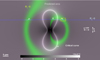 |
Fig. 1 Magnification map around a 1 M⊙ embedded in a macrolens potential with magnification µt = 100 and µr = 2. The gray scale shows the magnification with the critical curve around the microlens forming a standing hourglass figure. The blue, almost horizontal, thin curve marks the region where the residual Ry ~ 0. The wide green curve marks the corresponding region where the residual Rx ~ 0. Arcs form in regions where both blue and green curves overlap, that is, when the condition in Eq. (3) is satisfied. The yellow rectangle encloses a small region shown in the cartoon representation of Fig. 2. The gray scale shows the logarithm of the magnification. The direction of the tangential and radial components of the magnification are marked in the horizontal and vertical direction respectively. |
2.2 Interpolating at the subpixel level
In the previous section, we show the simple example of a microlens producing three microimages. The pixels potentially containing microimages can be rapidly found by restricting the search to pixels, where d2 is below some threshold ϵ, for instance ϵ = 100 R* or more generally ϵ < 1 pixel. The set of pixels that meet this requirement needs to be updated only a few times, since changes in d are very small when the source position is varied by a distance comparable to R*, and much smaller than the pixel size. Restricting the search of microimages to the subset of pixels that satisfy d < ϵ, and given the smooth (and linear) dependency of d, Rx, and Ry with the source position, the small subsample of pixels containing microimages can be easily identified, since Rx and Ry must cross within that pixel; or equivalently d must contain a zero, that is, the quantity Rx − Ry changes sign between two opposing edges in the pixel. This change of sign can be easily computed by interpolating neighboring pixels left and right of the pixel being tested. After the preselection of pixels containing a zero (or crossing between the lines Rx = 0 and Ry = 0) is performed, the last element that remains is the determination of the magnification of the microimages within each one of these pixels.
Through a combination of linear interpolations, it is possible to determine the size of the microimage within a pixel and, hence, the magnification. For circular sources such as stars, the intrinsic size of the source is given by  and the magnification of the microimage, i, is given by
  , where Ai is the estimated area of the microimage, i. By adding up the magnifications from all individual microimages, we can compute the net magnification for that particular position, (βx, βy), of the source.
Taking advantage of the smoothness of the deflection field, we can interpolate it to find the fraction of a pixel that contains a counterimage. A cartoon representation of the different steps in the algorithm is given in Figs. 2 and 3.
The size (or area Ai) of the microimage can be estimated by computing the four points HA, HB, HC, and HD shown in Fig. 3 as the intersecting points between the lines Rx = ± R* and Ry = ± R,.
Alternatively, we can also use the intersection points H1, H2, H3, and H4. The magnification of each microimage is found by computing the ratio of areas:
 (4)
(4)
where Ap is the area of the parallelogram defined by the intersection points HA, HB, HC, and HD. This area needs to be corrected by the factor of π/4 to account for the fact that the lensed image does not occupy the entire area within the parallelogram. The area Ai is then given by;
 (5)
(5)
where d(H3, H4) is the distance between these points, and h is the distance between the two lines Rx = R* and Rx = −R*. This distance is given by;
 (6)
(6)
where Sx is the slope of the line Rx = 0 and y1, y2 are constants in the relation y = y12 + Sx x, which are determined through interpolation. The point y1 is obtained as the point where Rx = R. between pixels (i, j + 1) and (i, j − 1). Similarly, the point y2 can be obtained as the position where Rx = −R*. between the same pixels.
The algorithm described above can be used to compute the magnification of a given source. We have ignored intrinsic variability in the luminosity of the source (for instance a variable star) or its radius (for instance, a supernova). For these types of objects, the light curve is a product of the magnification times the intrinsic luminosity of the object, which can vary over time. For the particular case of a supernova with an expanding photosphere crossing a microcaustic, the change in radius needs to be factored in when computing the magnification of areas in Eq. (4).
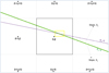 |
Fig. 2 Representation of Rx and Ry at the subpixel area. The squares represent the pixel size. The pixel at position (i, j), and containing a microimage is marked with thicker solid black lines in the center. Neighboring pixels are marked with dashed lines. The residual Ry and Rx are marked with blue and green lines, respectively. The yellow rectangle is the region represented in greater detail in Fig. 3. |
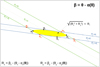 |
Fig. 3 Cartoon representation of the algorithm. Points H1 through H4 are found through interpolation of the smooth Rx and Ry 2D fields, as the intersection points at Rx,y = 0, ±R*. The scale of the pixel is not shown but is assumed to be much larger than the size of this figure (see Fig. 2). |
3 Comparison with ray tracing
In order to test the performance of the algorithm we compute the deflection field with a pixel scale of 30 nanoarcsec per pixel and place a microlens in the center with 1 M⊙ (see Fig. 1). For the background star, we adopted a radius of 20 R⊙, that is, the star is ≈2500 times smaller in area than the pixel. Resolving this star with a standard ray tracing algorithm would require a simulation having 25002 = 6.25 million times more pixels. The computation of the deflection field alone for the simplest cases shown in this work take approximately 1 minute. At the resolution of a 20 R⊙ star the same deflection field would take 6.25 million times longer, or ≈12 yr.
The star moves in a horizontal direction with respect to the microlens shown in Fig. 1 and forms microimages along the Ry = 0 region shown in the same figure. We compute the net magnification at each source position by adding the magnification of each microimage using the algorithm described above. The result is shown in Fig. 4 as a black solid line. In a regular laptop, it takes less than a minute to compute this light curve (1000 varying star positions in the source plane). For comparison we show as a red dashed line the result obtained from the brute force approach of inverse ray shooting, where the magnification is computed in the source plane after shooting rays back from the image plane. The standard ray shooting technique cannot resolve the caustics well and predicts smaller magnification values. In contrast, our fast algorithm is able to properly resolve the caustics, even for sources as small as R = 20 R⊙.
We also tested the capability of the new algorithm to resolve small microlenses. We placed a small microlens with one Jupiter mass (or ≈0.001 M⊙) near the caustic at ≈0.1 µarcsec. In the image plane, this small microlens is at a physical distance of ≈0.1 parsec from the larger microlens, so it should be interpreted as a rogue planet that is not gravitationally bound to the larger microlens. The critical curve of the Jupiter mass microlens is amplified by the combined magnification of the 1 M⊙ microlens and the galaxy (or cluster) macrolens. In Fig. 5, we show the light curve when the path of the background star intersects the small microcaustic from the rogue planet. For this particular case, we considered an even smaller background star with radius R = 5 R©. The new algorithm is able to resolve both – namely, the smaller Jupiter mass microlens and the smaller background star. As in Fig. 5, the red dashed line corresponds to the standard ray shooting technique that cannot resolve the small microlens and fails at reproducing the magnification during the caustic crossing. The example shown in Fig. 5 also serves to illustrate the limitations of the new algorithm, since small artifacts can be appreciated near the Jupiter mass microcaustic. In this case, the assumption made about the linear behaviour of the deflection field within the 30 nanoarcsec simulation pixel is not as accurate as in the case of the larger microlens. To better reproduce this case, a cubic interpolation or a smaller pixel size may be necessary. Nevertheless, this test is useful to show that the algorithm can be used to efficiently produce light curves when a wide range of microlens masses are involved. Additional light curves can be found in the original paper that made use of this algorithm for the first time (Diego et al. 2018).
As a final example, we consider the case of a crowded field with a surface mass density of microlenses, Σ, similar to what can be found in realistic situations. In typical lensing systems, the critical surface mass density is Σc ≈ 2000 M⊙ pc−2. Around these critical curves, the stars in the intracluster light are not expected to contribute more than a fraction of a percent to the total projected mass so we assume a convergence for the microlenses of κ* = 10−3 or Σc ≈ 2000 M⊙ pc−2 for Σc ≈ 2000 M⊙ pc−2. As in the previous cases, we fixed the macromodel magnification to µ = µt × µr = 200 × 2 = 200. The performance of the algorithm for a background star of 20 solar radii is shown in Fig. 6 as a black solid line, where it is compared with the result that would have been obtained from the standard inverse ray shooting at resolution of 30 nas per pixel (red curve). The inset figure in the middle shows the microcaustics in the source plane. The trajectory of the background star through the web of microcaustics is marked with a straight line in the inset figure. The star is moving from left to right. Near the microcaustics, the inverse ray shooting (red line) cannot resolve the fine details. The difference between the new algorithm and the ray shooting can be better appreciated if we zoom in around one of the peaks shown in Fig. 6. We select the peak near position -0.5 microarcsec in Fig. 6 and run this portion of the light curve with smaller time steps. The result is shown in Fig. 7, where we show again the ray shooting result in red. For reference we show as a blue horizontal line the distance traveled by a source at z = 2 during one month when its moving at a relative speed of 1000 km s−1. The new method can easily resolve time intervals smaller than one day while the ray shooting method cannot resolve time intervals smaller than ≈2 months.
Small artifacts (mostly negative small fluctuations) can still be appreciated in Fig. 6, especially in regions of high density of microlenses. These artifacts can be easily corrected since negative fluctuations similar to these ones are not expected and can be easily identified (and removed). Alternatively, we can consider higher order interpolations of the deflection field since, in regions of high density of microlenses, the approximation that the deflection field is exactly linear may not be as accurate.
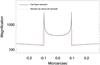 |
Fig. 4 Comparison with standard ray shooting. The solid line shows the result from our method for a star with R = 20 R⊙. For comparison we show as a red dotted line the result obtained from the ray-shooting method, with a pixel scale similar to the one used for the simulation in the image plane (30 nanoarcsec). The trajectory of the star intersects the microcaustic horizontally. The microlens has one solar mass and microimages form along the curve Ry = 0 shown in Fig. 1. |
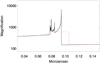 |
Fig. 5 Zoom-in near a caustic with a rogue planet acting as a perturber near the larger microlens. This plot shows a small portion of the critical curve for the same trajectory and microlens as in Fig. 4 but where a small perturber with mass equal to one Jupiter mass intersects the trajectory of the counterimages near the right peak at ≈0.1 microarcsec in Fig. 4. For this plot, the background star is also smaller with radius R = 5 R⊙. The red dotted lines shows the result obtained with the ray shooting method that does not resolve the small mass perturber. |
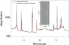 |
Fig. 6 Example of a light curve in a crowded field. The surface mass density of microlenses is ≈2 M⊙ pc−2, a typical value responsible for the intracluster light (ICL) near the tangential critical curves of high redshift sources. The black solid line shows the light curve for a 20 solar radii background star and it is compared with the ray tracing solution (red curve) for a resolution of 30 nas per pixel. As in the previous examples, ray tracing cannot capture the fine details near the microcaustics. The 2D image in the center shows the magnification map in the source plane and the straight line marks the trajectory of the background star across the field of microcaustics. |
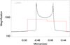 |
Fig. 7 Zoom-in at increased temporal resolution around the peak at ≈−0.5 microarcsec in Fig. 6. The blue horizontal line in the top-left part of the figure shows the distance traveled during one month by a source at z = 2 moving at 1000 km s−1 in relation to the microcaustics. |
4 Conclusions
We present a new algorithm to compute light curves of stars grazing a field of microcaustics near the caustic of a galaxy or cluster macrolens. In these scenarios, given the large magnification factors, µm, from the macrolens (typically hundreds to thousands), the simulated region in the image plane needs to be relatively large. In the source plane, this large region gets compressed by the factor µm. If a luminous star is moving at a typical relative velocity of ~ 1000 km s−1 with respect to the micro-caustic network, it can cover ≈1 microarcsec in the source plane over 10 yr. The corresponding microimages would span a region µm times larger in the image plane. This means that in realistic scenarios, the simulated region must cover approximately 1 milliarcsec in the image plane. If we want to resolve the magnification of stars (with typical sizes ~10−11″) with standard ray shooting techniques, the number of pixels to be simulated would be prohibitive. In this work, we present an algorithm that relies on the smoothness of the deflection field in order to resolve microimages at the subpixel level. Using simulations with a pixel size that is several orders of magnitude greater than the size of the stars, we show how it is possible to quickly reproduce the light curves of a star moving across a web of microcaustics. The method is fast (less than 1 min using a basic laptop for 1000 positions in the source plane) and accurate. We show how stars at cosmological distances as small as 5 R⊙, or time intervals smaller than 1 day, can be resolved when the original simulation is done with a 30 nanoarcsec pixel. We also show how small microlenses with masses comparable to planets can be also resolved by the algorithm.
Acknowledgements
We thank the anonymous referee for carefully reviewing the manuscript and providing useful comments and feedback. J.M.D. acknowledges the support of project PGC2018-101814-B-100 (MCIU/AEI/MINECO/FEDER, UE) Ministerio de Ciencia, Investigation y Universidades. This project was funded by the Agencia Estatal de Investigaciön, Unidad de Excelencia Maria de Maeztu, ref. MDM-2017-0765.
References
- Chang, K., & Refsdal, S. 1979, Nature, 282, 561 [Google Scholar]
- Chen, W., Kelly, P. L., Diego, J. M., et al. 2019, ApJ, 881, 8 [NASA ADS] [CrossRef] [Google Scholar]
- Coe, D., Salmon, B., Bradac, M., et al. 2019, ApJ, 884, 85 [NASA ADS] [CrossRef] [Google Scholar]
- Diego, J. M. 2019, A&A, 625, A84 [NASA ADS] [CrossRef] [EDP Sciences] [Google Scholar]
- Diego, J. M., Kaiser, N., Broadhurst, T., et al. 2018, ApJ, 857, 25 [NASA ADS] [CrossRef] [Google Scholar]
- Diego, J. M., Pascale, M., Kavanagh, B. J., et al. 2022, A&A, in press https://doi.org/10.1051/0004-6361/202243605 [Google Scholar]
- Esteban-Gutiérrez, A., Mediavilla, E., Jiménez-Vicente, J., et al. 2022, ApJ, 929, L17 [CrossRef] [Google Scholar]
- Irwin, M. J., Webster, R. L., Hewett, P. C., Corrigan, R. T., & Jedrzejewski, R. I. 1989, AJ, 98, 1989 [NASA ADS] [CrossRef] [Google Scholar]
- Kaurov, A. A., Dai, L., Venumadhav, T., Miralda-Escudé, J., & Frye, B. 2019, ApJ, 880, 58 [NASA ADS] [CrossRef] [Google Scholar]
- Kelly, P. L., Diego, J. M., Rodney, S., et al. 2018, Nat. Astron., 2, 334 [NASA ADS] [CrossRef] [Google Scholar]
- Meena, A. K., Arad, O., & Zitrin, A. 2022, MNRAS, 514, 2545 [CrossRef] [Google Scholar]
- Ohyama, Y., & Hota, A. 2013, ApJ, 767, L29 [NASA ADS] [CrossRef] [Google Scholar]
- Paczynski, B. 1986, ApJ, 301, 503 [NASA ADS] [CrossRef] [Google Scholar]
- Rodney, S. A., Balestra, I., Bradac, M., et al. 2018, Nat. Astron., 2, 324 [Google Scholar]
- Vanzella, E., Meneghetti, M., Pastorello, A., et al. 2020, MNRAS, 499, L67 [CrossRef] [Google Scholar]
- Venumadhav, T., Dai, L., & Miralda-Escudé, J. 2017, ApJ, 850, 49 [NASA ADS] [CrossRef] [Google Scholar]
- Welch, B., Coe, D., Diego, J. M., et al. 2022, Nature, 603, 815 [NASA ADS] [CrossRef] [Google Scholar]
- Witt, H. J. 1993, ApJ, 403, 530 [NASA ADS] [CrossRef] [Google Scholar]
A JWST program to observe Earendel is already approved.
All Figures
|
Fig. 1 Magnification map around a 1 M⊙ embedded in a macrolens potential with magnification µt = 100 and µr = 2. The gray scale shows the magnification with the critical curve around the microlens forming a standing hourglass figure. The blue, almost horizontal, thin curve marks the region where the residual Ry ~ 0. The wide green curve marks the corresponding region where the residual Rx ~ 0. Arcs form in regions where both blue and green curves overlap, that is, when the condition in Eq. (3) is satisfied. The yellow rectangle encloses a small region shown in the cartoon representation of Fig. 2. The gray scale shows the logarithm of the magnification. The direction of the tangential and radial components of the magnification are marked in the horizontal and vertical direction respectively. |
| In the text | |
|
Fig. 2 Representation of Rx and Ry at the subpixel area. The squares represent the pixel size. The pixel at position (i, j), and containing a microimage is marked with thicker solid black lines in the center. Neighboring pixels are marked with dashed lines. The residual Ry and Rx are marked with blue and green lines, respectively. The yellow rectangle is the region represented in greater detail in Fig. 3. |
| In the text | |
|
Fig. 3 Cartoon representation of the algorithm. Points H1 through H4 are found through interpolation of the smooth Rx and Ry 2D fields, as the intersection points at Rx,y = 0, ±R*. The scale of the pixel is not shown but is assumed to be much larger than the size of this figure (see Fig. 2). |
| In the text | |
|
Fig. 4 Comparison with standard ray shooting. The solid line shows the result from our method for a star with R = 20 R⊙. For comparison we show as a red dotted line the result obtained from the ray-shooting method, with a pixel scale similar to the one used for the simulation in the image plane (30 nanoarcsec). The trajectory of the star intersects the microcaustic horizontally. The microlens has one solar mass and microimages form along the curve Ry = 0 shown in Fig. 1. |
| In the text | |
|
Fig. 5 Zoom-in near a caustic with a rogue planet acting as a perturber near the larger microlens. This plot shows a small portion of the critical curve for the same trajectory and microlens as in Fig. 4 but where a small perturber with mass equal to one Jupiter mass intersects the trajectory of the counterimages near the right peak at ≈0.1 microarcsec in Fig. 4. For this plot, the background star is also smaller with radius R = 5 R⊙. The red dotted lines shows the result obtained with the ray shooting method that does not resolve the small mass perturber. |
| In the text | |
|
Fig. 6 Example of a light curve in a crowded field. The surface mass density of microlenses is ≈2 M⊙ pc−2, a typical value responsible for the intracluster light (ICL) near the tangential critical curves of high redshift sources. The black solid line shows the light curve for a 20 solar radii background star and it is compared with the ray tracing solution (red curve) for a resolution of 30 nas per pixel. As in the previous examples, ray tracing cannot capture the fine details near the microcaustics. The 2D image in the center shows the magnification map in the source plane and the straight line marks the trajectory of the background star across the field of microcaustics. |
| In the text | |
|
Fig. 7 Zoom-in at increased temporal resolution around the peak at ≈−0.5 microarcsec in Fig. 6. The blue horizontal line in the top-left part of the figure shows the distance traveled during one month by a source at z = 2 moving at 1000 km s−1 in relation to the microcaustics. |
| In the text | |
Current usage metrics show cumulative count of Article Views (full-text article views including HTML views, PDF and ePub downloads, according to the available data) and Abstracts Views on Vision4Press platform.
Data correspond to usage on the plateform after 2015. The current usage metrics is available 48-96 hours after online publication and is updated daily on week days.
Initial download of the metrics may take a while.