| Issue |
A&A
Volume 697, May 2025
|
|
|---|---|---|
| Article Number | A194 | |
| Number of page(s) | 14 | |
| Section | Cosmology (including clusters of galaxies) | |
| DOI | https://doi.org/10.1051/0004-6361/202453234 | |
| Published online | 16 May 2025 | |
DUCA: Dynamic Universe Cosmological Analysis
I. The halo mass function in dynamical dark energy cosmologies
1
INAF – Osservatorio Astronomico di Trieste, Via G. B. Tiepolo 11, 34143 Trieste, Italy
2
INFN – Sezione di Trieste, Via Valerio 2, 34127 Trieste TS, Italy
3
IFPU – Institute for Fundamental Physics of the Universe, via Beirut 2, 34151 Trieste, Italy
4
ICSC, Via Magnanelli 2, Bologna, Italy
5
Dipartimento di Fisica – Sezione di Astronomia, Università di Trieste, Via Tiepolo 11, Trieste 34131, Italy
6
Department of Astrophysics – University of Zurich, Winterthurerstrasse 190, 8057 Zürich, Switzerland
⋆ Corresponding author: tiago.batalha@inaf.it
Received:
29
November
2024
Accepted:
9
April
2025
Context. The halo mass function (HMF) is fundamental for interpreting the number counts of galaxy clusters and serves as a pivotal theoretical tool in cosmology. With the advent of high-precision surveys such as LSST, eROSITA, DESI, and Euclid, accurate HMF modeling becomes indispensable in order to avoid systematic biases in cosmological parameter estimation from cluster cosmology. Moreover, these surveys aim to shed light on the dark sector and uncover dark energy’s (DE) puzzling nature; thus they necessitate models that faithfully capture DE’s features to ensure robust parameter inference.
Aims. We aim to construct a model for the HMF in dynamical DE cosmologies that preserves the accuracy achieved for the standard Λ(ν)CDM model of cosmology while meeting the precision requirements necessary for future cosmological surveys.
Methods. Our approach models the HMF parameters as functions of the deceleration parameter at the turnaround, a quantity that has been shown to encapsulate essential information regarding the impact of dynamical DE on structure formation. We calibrated the model using results from a comprehensive suite of N-body simulations spanning various cosmological scenarios, which ensured subpercent systematic accuracy.
Results. We present a HMF model tailored for dynamical DE cosmologies. The model was calibrated following a Bayesian approach, and its uncertainty is characterized by a single parameter controlling its systematic error, which remains at the subpercent level. This ensures that theoretical uncertainties from our model are subdominant relative to other error sources in future cluster number count analyses.
Key words: cosmology: theory / dark energy / large-scale structure of Universe
© The Authors 2025
 Open Access article, published by EDP Sciences, under the terms of the Creative Commons Attribution License (https://creativecommons.org/licenses/by/4.0), which permits unrestricted use, distribution, and reproduction in any medium, provided the original work is properly cited.
This article is published in open access under the Subscribe to Open model. Subscribe to A&A to support open access publication.
1. Introduction
Structure formation in the Universe proceeds hierarchically, with small-scale perturbations collapsing and merging to form larger structures over cosmic time. Galaxy clusters, being the most massive virialized objects, sit at the apex of this hierarchy and serve as powerful probes of cosmology (see reviews by Allen et al. 2011; Kravtsov & Borgani 2012). The abundance and distribution of galaxy clusters provide valuable cosmological information, including on the growth of cosmic structures and the nature of dark energy (DE) (Borgani et al. 2001; Schuecker et al. 2003; Majumdar & Mohr 2004; Vikhlinin et al. 2009; Planck Collaboration XXIV 2016; Marulli et al. 2018; Bocquet et al. 2019; Costanzi et al. 2021; Fumagalli et al. 2024).
The halo mass function (HMF), which describes the comoving number density of dark matter halos as a function of mass and redshift, is a key theoretical tool for interpreting observations of galaxy clusters (e.g., Press & Schechter 1974; Bond et al. 1991; Sheth & Tormen 1999; Sheth et al. 2001; Tinker et al. 2008; Despali et al. 2016; Bocquet et al. 2020; Ondaro-Mallea et al. 2021; Euclid Collaboration: Castro et al. 2023). Accurate modeling of the HMF is essential for not biasing the constraints on cosmological parameters from cluster surveys (e.g., Salvati et al. 2020; Artis et al. 2021).
Due to their non-linearity, accurate and precise modeling of the HMF requires simulations that fully capture the non-linear evolution of cosmic structures. Notably, N-body simulations (see Angulo & Hahn 2022, for a review) provide a theoretical means to examine the non-linear regime at which galaxy clusters are entangled, but they operate under the assumption that baryonic feedback is subdominant to gravity. Despite being a minor component in our Universe, different studies have shown that luminous matter significantly affects structure formation in the Universe (Cui et al. 2014; Velliscig et al. 2014; Bocquet et al. 2016; Castro et al. 2020; Euclid Collaboration: Castro et al. 2024a). At the scale of galaxy clusters, it is well understood that baryonic feedback does not disrupt structures; instead, it redistributes the halo’s composition, altering its mass compared to the same object simulated with a collisionless scheme. Given that hydrodynamical simulations are substantially more computationally demanding than purely gravitational N-body simulations, the commonly adopted approach is to characterize the HMF using the latter and then to model the impact of baryonic physics on halo masses in post-processing (see, e.g., Schneider & Teyssier 2015; Aricò et al. 2021; Euclid Collaboration: Castro et al. 2024a). The baryonic implications in the HMF are not addressed in the rest of this paper.
In the standard cosmological model, Λ cold dark matter (CDM), the accelerated expansion of the Universe is driven by a cosmological constant (Λ). However, the physical nature of DE remains one of the biggest challenges in modern cosmology. Dynamical DE models (see, for instance, Peebles & Ratra 2003; Copeland et al. 2006), where the DE equation of state evolves with time, offer alternatives to the cosmological constant and can leave distinct signatures on the formation and evolution of cosmic structures (Frieman et al. 2008; Weinberg et al. 2013).
Ongoing and upcoming missions such as the Vera C. Rubin Observatory’s Legacy Survey of Space and Time (LSST; LSST Science Collaborations 2009)1, the third generation of the South Pole Telescope (SPT-3G; Benson 2014)2, the DE Spectroscopic Instrument (DESI; DESI Collaboration 2016)3, the Nancy Grace Roman Space Telescope (Spergel et al. 2015)4, the Square Kilometre Array (SKA; Maartens et al. 2015)5, eROSITA (Predehl et al. 2021)6, and Euclid (Euclid Collaboration: Mellier et al. 2025)7 will provide unprecedented observations of the large-scale structure of the Universe and will help to shed light on the nature of the dark sector. These surveys will push the statistical uncertainties to never-before-seen levels, and theoretical models must keep pace.
Understanding how dynamical DE affects the HMF is therefore crucial for extracting accurate cosmological information from current and future surveys of galaxy clusters. Previous studies have explored the impact of different DE features on the HMF (e.g., Courtin et al. 2011; Cui et al. 2012; Bhattacharya et al. 2011; Sáez-Casares et al. 2024; Shen et al. 2025), often finding that variations in its dark nature can lead to significant differences in the predicted abundance of massive halos, especially at low redshifts, when the dynamics of the Universe are driven by DE. While these works have modeled the HMF in different scenarios, the diversity of dynamical DE models and the precision requirements of upcoming surveys necessitate further work to keep pace in accuracy and precision with the available predictions for the HMF in the ΛCDM.
In this work, we extend our previous study on the HMF (Euclid Collaboration: Castro et al. 2023) to dynamical DE models described by the Chevallier–Polarski–Linder (CPL) parametrization (Chevallier & Polarski 2001; Linder 2003). The CPL framework provides a widely used phenomenological model that describes the DE equation of state w(a) as a linear function of the scale factor a with two parameters: w0, which is the present-day value of wDE, and wa, which characterizes its evolution. We aim to calibrate a new model for the HMF that accounts for the effects of a time-varying DE equation of state while retaining the accuracy needed for the analysis of upcoming cluster surveys to ensure that theoretical uncertainties do not dominate the error budget.
To this end, we performed a series of precise N-body simulations spanning various cosmologies. We analyzed the resulting halo catalogs to quantify the impact of dynamical DE on the HMF and to develop a fitting function that accurately reproduces the simulation results across the parameter space.
This paper is organized as follows: In Sect. 2, we present the theoretical framework, focusing on the w0wa model and the HMF. In Sect. 3, we describe the methodology used for calibrating the HMF model, including the simulation setup and the Bayesian approach for parameter estimation. In Sect. 4, we present our results, highlighting the accuracy and robustness of the proposed model compared to other existing models. Our conclusions are drawn in Sect. 5. Finally, the python implementation of our model is presented in Data availability section8.
2. Theory
In this section, we present a short overview of the main concepts used in this paper. We review the CPL model in Sect. 2.1 and the HMF in Sect. 2.2.
2.1. The w0wa cold dark matter model
The CPL model (Chevallier & Polarski 2001; Linder 2003) is a phenomenological approach to describe the evolution of the DE equation of state parameter wDE that determines the relation between the pressure and density of the DE, p = wDEρc2. It is expressed as a function of the scale factor a as

or equivalently in terms of redshift as
where w0 is the present-day value of the DE equation of state and wa is its rate of change with respect to the scale factor.
In a flat universe including matter, radiation, massive neutrinos, and DE components, the Hubble parameter H(z) is given by
where H is the Hubble constant and H0 is its value at the present day; Ωm, 0, Ωr, 0, and ΩDE, 0 are the present-day density parameters for matter (including both baryonic and CDM), radiation, and DE. The term Ων(z) is the neutrino density parameter at redshift z, ρc(z) is the critical density at redshift z, and ρc, 0 is its value at the present day.
The integral in the exponential in Eq. (3) accounts for the evolution of DE density due to its dynamic equation of state. Using the w0wa parametrization, the exponential term becomes (Linder 2003)

Standard massive neutrinos play a unique role in cosmology, affecting both the background expansion and the growth of cosmic structures (Lesgourgues & Pastor 2006). The present-day value of the neutrino density parameter Ων, 0 depends on the sum of the masses of the three neutrino species ∑mν and is approximately given by
where h = H0/(100 km s−1 Mpc−1). At early times (z ≫ 1), neutrinos behave similarly to radiation ( ), while at late times ( z ≲ 1), they become non-relativistic and act similarly to a pressureless fluid (wν = 0). Lastly, massive neutrinos are known to follow a hierarchy in their masses, with possible normal or inverted ordering (Lesgourgues & Pastor 2006). However, for simplicity, we assume in the rest of this work that all three neutrino species have the same mass.
The main feature of DE models is explaining the currently observed accelerated expansion of the Universe. The deceleration parameter qdec the variation of the expansion rate and is defined as (Weinberg 2008; Peebles 2020)
where the dots denote derivatives with respect to cosmic time.
Using the Friedmann equations, qdec can be expressed in terms of the density parameters and their respective equations of state:
![$$ \begin{aligned} q_{\rm dec}(z) = \frac{1}{2} \sum _i \Omega _i(z) \left[ 1 + 3 w_i(z) \right], \end{aligned} $$](/articles/aa/full_html/2025/05/aa53234-24/aa53234-24-eq8.gif)
where the sum runs over all components i (matter, radiation, neutrinos, DE) and wi(z) is the equation of state parameter for each component:
-
wm = 0 for matter.
-
 for radiation.
 -
wν(z) for neutrinos, transitioning from
 to 0.
to 0. -
wDE(z) given by the CPL model for DE.
At the present time (z = 0), the deceleration parameter is approximately
![$$ \begin{aligned} q_{\rm dec,0} \approx \frac{1}{2} \left[ 2\,\Omega _{\rm m,0} + \Omega _{\rm {DE},0} (1 + 3 w_0) \right]. \end{aligned} $$](/articles/aa/full_html/2025/05/aa53234-24/aa53234-24-eq11.gif)
Thus, a negative value of qdec indicates cosmic acceleration, while a positive value indicates deceleration. Since the deceleration parameter is measured to be negative at the present time, a necessary condition for this acceleration is that the equation of state parameter satisfies w0 < −1/3.
2.2. The halo mass function
The comoving number density of dark matter halos within the mass range [M, M + dM] is described by the differential HMF
where ρm is the mean comoving matter density of the Universe, ν is the peak height parameter, and νf(ν) is known as the multiplicity function. The peak height ν quantifies the rarity of a halo and is defined as

with δc being the critical density threshold for spherical collapse linearly extrapolated to redshift z and σ(M, z)2 representing the mass variance at redshift z. The mass variance is computed from the linear matter power spectrum Pm(k, z) via
where R(M) is the Lagrangian radius corresponding to mass M, given by R = (3M/4πρm)1/3, and W(kR) is the Fourier transform of the real-space top-hat window function.
In cosmologies with massive neutrinos, the structure formation is tightly connected to the CDM plus baryons density field instead of the total density field including the neutrino contribution (Castorina et al. 2014; Costanzi et al. 2013; Vagnozzi et al. 2018). Therefore, in this scenario, it is necessary that the matter field considered in the comoving matter density field ρm in Eq. (9) and the matter power spectrum Pm in Eq. (11) refers to the CDM plus baryons only to evaluate the model correctly (see also Euclid Collaboration: Castro et al. 2023, 2024b).
The assumption of universality implies that the multiplicity function νf(ν) is independent of cosmology when expressed in terms of the peak height ν. While this holds approximately, several studies using N-body simulations have identified systematic deviations from universality, especially at late times (Crocce et al. 2010; Courtin et al. 2011; Watson et al. 2013; Diemer 2020; Ondaro-Mallea et al. 2021).
These deviations have been attributed to factors such as the specific definition of halos (Watson et al. 2013; Despali et al. 2016; Diemer 2020; Ondaro-Mallea et al. 2021) and a residual cosmology dependence of the collapse threshold δc. For instance, Courtin et al. (2011) demonstrated that accounting for the cosmological variation of δc leads to a more universal HMF, particularly at the high-mass end, which is critical for cluster cosmology.
In our analysis, we define halos using the spherical overdensity (SO) criterion, where halos are spheres within which the mean density is Δvir(z) times the background matter density. The value of the virial overdensity Δvir(z) and its dependence on cosmological parameters are determined by the spherical collapse model solution (Eke et al. 1996).
We adopted the fitting formula for Δvir(z) presented by Bryan & Norman (1998) even though it was calibrated for ΛCDM cosmologies, and the results for dynamical DE models can differ significantly when derived from the numerical solution of the spherical collapse. The rationale behind this choice is threefold. First, this definition has already been implemented in several halo finders for practicality. Second, numerically solving the spherical collapse for arbitrary dynamical DE fluids poses several technical (Pace et al. 2017) and physical (Batista 2021) challenges. Third, we aim for our HMF model to be computationally efficient so that it does not add a computational load during cluster cosmology likelihood computations. Nonetheless, we are confident that using the solution for the virial threshold would likely preserve the universality of the HMF more effectively than the adopted definition, as has been observed previously for other definitions in ΛCDM cosmologies (Despali et al. 2016; Diemer 2020; Ondaro-Mallea et al. 2021).
We adopted the fitting function for the multiplicity function introduced by Euclid Collaboration: Castro et al. (2023) as a starting point for our modeling. This multiplicity function is given by
![$$ \begin{aligned} \nu f(\nu ) = A(p, q) \sqrt{\frac{2 a \nu ^2}{\pi }} \exp \left( -\frac{a \nu ^2}{2} \right) \left[ 1 + \frac{1}{(a \nu ^2)^p} \right] (\sqrt{a} \nu )^{q - 1}, \end{aligned} $$](/articles/aa/full_html/2025/05/aa53234-24/aa53234-24-eq15.gif)
where the parameters a, p, and q are functions of the cosmological background evolution and the shape of the matter power spectrum. Specifically, they are modeled as
with
Here, dlnσ/dlnR is the mass variance’s logarithmic slope as a function of the Lagrangian radius R.
The normalization constant A(p, q) is determined by the requirement that all matter is contained within halos, as prescribed by the halo model (Cooray & Sheth 2002). When the parameters a, p, and q are independent of ν, the normalization is given by
![$$ \begin{aligned} A(p, q) = \left\{ \frac{2^{-1/2 - p + q/2}}{\sqrt{\pi }} \left[ 2^p \Gamma \left( \frac{q}{2} \right) + \Gamma \left( -p + \frac{q}{2} \right) \right] \right\} ^{-1}, \end{aligned} $$](/articles/aa/full_html/2025/05/aa53234-24/aa53234-24-eq21.gif)
where Γ denotes the gamma function. It should be noted, however, that this normalization condition may not strictly hold in the real Universe (Angulo & White 2010). Our model uses Eq. (18) to ensure appropriate asymptotic behavior when extrapolating the HMF to lower masses, even though the parameters vary with cosmology and scale.
The values for the parameters {a1, a2, az, p1, p2, q1, q2, qz} are from Table 4 of Euclid Collaboration: Castro et al. (2023), and they were calibrated using the ROCKSTAR halo finder. We refer to that paper for a thorough discussion on the effect of changing the halo finder on the resulting HMF. Finally, for the cosmology-dependence of the critical density threshold δc, we employed the fitting formula provided by Kitayama & Suto (1996).
3. Methodology
In this section, we present the methodology used to calibrate the HMF model. In Sect. 3.1, we present the simulations used (Sect. 3.1), the halo finder is presented in Sect. 3.2, and the Bayesian analysis in Sect. 3.3.
3.1. Simulations
This work utilizes the Dynamic Universe Cosmological Analysis (DUCA) cosmological N-body simulation suite. This set of simulations was generated using the CoNcept code (Dakin et al. 2022)9, with detailed documentation available online10.
The initial conditions were created on the fly by CoNcept using the recently implemented third-order Lagrangian perturbation theory (3LPT) module at the initial redshift zin = 24. We adjusted the force split range from their default values in CoNcept to achieve a higher accuracy in our simulations. Table 1 lists the specific force parameters used in our simulations (see Dakin et al. 2022, for the precise definitions of each parameter).
Force parameters used in the DUCA set of simulations, including short-range and long-range force specifications.
The DUCA simulation set was designed to explore the impact of varying cosmological parameters on the large-scale structure with high precision and efficiency and is divided into the three subsets, which we describe below and overview in Table 2. We present the triangle plot with the values of the cosmological parameters assumed for Ωm, 0, ∑mν, h, log10As, ns, w0, and wa by the different subsets in Fig. 1. The ranges within which these parameters vary were deliberately chosen to be conservative, encompassing the constraints from multiple cosmological probes. All simulations incorporate the effects of massive neutrinos and DE perturbations at background and linear perturbation levels through a continual grid realization and with general relativistic effects fully accounted for (Dakin et al. 2019a). CoNcept also deploys a nonlinear solver for the continuity and Euler equations for massive neutrinos on a grid following the approach outlined by Dakin et al. (2019b). However, operating under this setup results in significant computational overhead. Furthermore, Adamek et al. (2023) showed that the linear approach is sufficient to reproduce the impact of massive neutrinos in the HMF at the subpercent level.
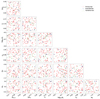 |
Fig. 1. Cosmological parameters for the three subsets of the DUCA simulations (see Sect. 3.1 for details). |
Summary of the simulation sets used in this work.
3.1.1. Primary simulation set
Our primary simulation set consists of 82 pairs of simulations. Each pair corresponds to different cosmological parameters. The cosmological parameters that we varied are Ωm, 0, Ωb, 0, ∑mν, H0, ns, As, w0, and wa.
These parameters were sampled using Latin hypercube sampling in order to efficiently cover the multidimensional parameter space. Each simulation has a comoving box size of 1 h−1 Gpc and contains 10243 dark matter particles, resulting in a particle mass resolution of approximately 2.6 × 10¹¹ (h/Ωm, 0)−1 M⊙. The simulations were evolved from redshift z = 24 to z = 0.
We employed fixed amplitudes and paired phases in the Fourier representation of the density fluctuation field for initial condition generation, following the method described by Angulo & Pontzen (2016). This technique generates pairs of simulations with initial power spectra that have an identical amplitude fixed at the mean P(k) value but with phases of the corresponding Fourier modes shifted by π. This approach effectively cancels the leading-order cosmic variance of clustering statistics when averaging over the pair.
3.1.2. Extended simulation sets
From the initial 82 cosmologies, we selected eight, as presented in Table 3. They were indexed according to their value of  . The cosmological parameters were selected by brute-force searching for the cosmological set that presented the largest variance. For these chosen cosmologies, we performed additional simulations to refine our HMF modeling further.
Cosmological parameters for the extended simulation set.
We ran eight pairs of large-volume simulations with the same mass resolution as the primary set but with a larger comoving box size of 2 h−1 Gpc. This increased the simulation volume and number of particles by a factor of eight, thus enhancing the statistics for massive halos and reducing the sample variance at the high-mass end.
We also ran eight pairs of high-resolution simulations with the same comoving box size and phases as the primary set (1 h−1 Gpc) but with an increased particle count of 20483. This improved the mass resolution by a factor of eight and allowed us to probe smaller-mass halos and better resolve the low-mass end of the HMF.
3.1.3. Validation simulations
In addition to the calibration simulations, we generated 20 independent simulations with random initial phases. These simulations have the same specifications as the primary set (1 h−1 Gpc box size and 10243 particles) but do not use paired phases. They serve as a validation set to test the predictive power of our HMF model. These simulations are not included in the calibration process to ensure an unbiased assessment of the model’s accuracy.
3.2. Halo finder
For our analysis, we employed the ROCKSTAR11 halo finder in combination with the CONSISTENT algorithm12. ROCKSTAR is a sophisticated phase-space halo finder that identifies halos by utilizing information from both the spatial and velocity distributions of particles (Behroozi et al. 2013a).
The ROCKSTAR algorithm initiates by partitioning the simulation volume into friends-of-friends (FoF) groups using a large (0.28) linking length compared to what is commonly used by other FoF-based algorithms (∼0.20). This partitioning facilitates efficient parallelization. Within each FoF group, ROCKSTAR performs an adaptive hierarchical refinement in six-dimensional phase space (three spatial dimensions and three velocity dimensions), creating a nested set of subgroups. This method allows for precise identification of halos and their substructures, even in densely populated regions of the simulation.
To enhance the temporal consistency and accuracy of the halo properties, we applied the CONSISTENT algorithm (Behroozi et al. 2013b) to the ROCKSTAR catalogs. CONSISTENT tracks halos across consecutive simulation snapshots, ensuring that properties such as halo masses and positions evolve smoothly over time. This dynamical tracking is crucial for reducing scatter and improving the reliability of halo catalogs, which is essential for our modeling.
We adopted the spherical overdensity (SO) definition for halos, with masses defined by an average density within a given sphere, which is equal to the virial overdensity Δvir(z) computed with respect to the background density, as described in Sect. 2.2. We included all particles within the virial radius in the halo mass calculation regardless of their gravitational binding.
The halo catalogs produced by ROCKSTAR plus CONSISTENT were binned logarithmically based on the number of particles per halo. This binning strategy minimizes the effects of mass discretization and ensures a statistically robust sampling across the halo mass spectrum.
3.3. Model calibration
This section outlines the Bayesian approach used to calibrate the HMF model. Our methodology closely follows that of Euclid Collaboration: Castro et al. (2023), and we refer to it for a comprehensive explanation. Here, we provide an overview of the key elements.
The calibration of the HMF involves fitting the theoretical model to the halo counts obtained from our suite of simulations described in Sect. 3.1. We assumed that the number of halos in each mass bin follows a Poisson distribution. This assumption was motivated by the Press–Schechter formalism (Press & Schechter 1974), where halo formation is treated as a random process driven by the collapse of matter overdensities. Therefore, the likelihood of observing Nisim halos in the i-th mass bin at redshift z is given by

where Nith = Ni(θ, z) is the theoretical prediction obtained by integrating the HMF model over the mass bin and multiplying by the simulation volume and θ represents the set of HMF model parameters.
However, in practice, systematic effects and numerical uncertainties can introduce additional scatter, especially in mass bins with many halos. To account for this, we adopted a composite likelihood approach where we approximated the Poisson distribution with a Gaussian distribution for bins with a sufficiently large number of halos (Euclid Collaboration: Castro et al. 2023). The composite log-likelihood is defined as
where σi is the standard deviation given by
Here, σsys represents an additional variance component accounting for systematic uncertainties. In contrast to Euclid Collaboration: Castro et al. (2023), we left σsys free to vary in our calibration.
The total log-likelihood used for the calibration was computed by summing over all mass bins, redshifts, and simulation outputs:
where the index s runs over all simulations. We assumed that the mass bins, redshifts, and simulations are statistically independent. Although outputs from the same simulation at different redshifts are not strictly independent due to the temporal correlation of structures, we mitigated this effect by selecting snapshots separated by time intervals larger than the typical dynamical time of galaxy clusters (approximately 1.7 Gyr) following the approach of Bocquet et al. (2016).
Robustly assessing the impact of correlation across redshifts would, in principle, require a large number of simulations with the same cosmology but different initial conditions, which goes beyond the scope of this paper. Instead, we performed a post hoc test by re-running the calibration after excluding every other selected redshift. Comparing the results of both calibrations revealed no statistically significant tension, ensuring that our final parameter constraints are robust concerning the chosen redshift binning scheme.
The total log-likelihood was sampled using EMCEE (Foreman-Mackey et al. 2013)13,14. A total of 896 walkers were used, each sampling 10 000 points. The walkers were initially set around a global maximum found by the DUAL ANNEALING algorithm (Tsallis 1988; Tsallis & Stariolo 1996; Xiang et al. 1997; Xiang & Gong 2000) implemented in SCIPY (Virtanen et al. 2020).
4. Results
In this section, we present our main results, starting with the modeling of the HMF, including the impact of resolution in our simulations in Sect. 4.1. We present the final baseline model in Sect. 4.2 and its calibration in Sect. 4.3. The assessment of the robustness is presented in Sect. 4.4, and a comparison with other models is given in Sect. 4.5.
4.1. Modeling
4.1.1. Resolution effects
It is important to assess the convergence of our simulations before modeling the impact of dynamical DE on the HMF. In Fig. 2, we present the difference between the HMF extracted from the primary set and their high-resolution counterpart. We present the results as a function of the number of particles Np in the primary simulation. We note that convergence at the 1% level is only achieved at all redshifts for objects with more than a thousand particles in our primary resolution.
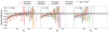 |
Fig. 2. Relative difference of the HMF extracted from the primary set to their high-resolution counterpart. We have labeled the cosmologies from the extended set according to their value of S8. The results are shown as a function of the number of particles Np in the primary simulation. |
We empirically calibrated the factor by which the HMF needs to be rescaled to account for the effect of resolution, that is, for the finite number of particles with which a halo is resolved:
Here, z is the redshift of a simulation snapshot. This correction factor is shown with dashed curves in Fig. 2. We verified that this correction factor is universal. In other words, it depends only on the number of halo particles but not on the simulated cosmology, which is within the range considered here. We also warn that this correction factor is calibrated for the range of redshifts relevant to our analysis. For the rest of the paper, when using the outcomes from the simulations with lower resolution, we tacitly correct them using Eq. (23). We also impose a minimum halo mass cut corresponding to 200 particles.
4.1.2. Baseline model
In Euclid Collaboration: Castro et al. (2023), we demonstrated that the multiplicity function presented in Eq. (12) is sufficiently flexible to accurately fit the results of several scale-free simulations. Consequently, their task of modeling the non-universality of the HMF was reduced to modeling the cosmological dependence of the free parameters in Eq. (12). We aim to follow a similar approach by starting with a baseline model and then modeling its cosmological dependence. However, the DUCA simulation set offers a significantly larger dynamical range to be fit, and we found that the same baseline model was not flexible enough to capture the simulation data accurately.
To address this limitation, we assessed the flexibility of different fitting functions by comparing each of them to a single catalog at redshift z = 0 from one pair of high-resolution simulations. Although the final model was not calibrated using the high-resolution simulations, this test served as a control to evaluate the overall flexibility of the fitting functions, as the high-resolution simulations provide a larger dynamical range. Empirically, we found that the following fitting function provides accurate results:
where  . In the above equation, the expression of the HMF normalization A is given by
with
Equation (24) reduces to Eq. (12) in the limit r → 0 and νp → 1. The rationale behind these modifications is to increase the model’s flexibility by introducing a double power-law behavior controlled by the parameter r and incorporating a different pivot scale νp.
4.1.3. Cosmological dependency of {a, p, q, r, vp}
In Euclid Collaboration: Castro et al. (2023), we show how the cosmological dependency of the HMF parameters {a, p, q} can be modeled as a function of the parameters determining the Friedman background and the shape of the power spectrum. It is natural to impose that the extension allowed by the parameter r behaves similarly to the parameter p (see Eq. (15)), as they operate over a similar range in ν. Therefore, we assumed that
while we assumed νp to be a constant in order not to introduce unwanted degeneracies with the parameter a.
To visually inspect the impact of dynamical DE on the HMF, we present in Fig. 3, a comparison between the HMF predictions by the model of Euclid Collaboration: Castro et al. (2023) and the observed HMF on the extended large simulations for three different redshifts z ∈ {0.00, 1.18, 1.98}. In the top panel, we observed that the model of Euclid Collaboration: Castro et al. (2023) qualitatively agrees with the simulations. The differences reported in the bottom panel amount to only a few percent even though the simulations analyzed here involve a wider dynamic range and a different range of cosmological parameters than those the HMF calibration in Euclid Collaboration: Castro et al. (2023) is based on. Interestingly, we noted that the differences between the model and the simulations are higher at lower redshift when the background evolution is dominated by DE.
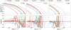 |
Fig. 3. Top: Comparison between the HMF predicted by the model of Euclid Collaboration: Castro et al. (2023) (curves) and the HMF measured for the extended large simulations (points). Error bars associated with each simulation point correspond to the Poisson uncertainty. Bottom: Relative difference between the model and the simulations. Different panels indicate different redshifts; from left to right, z = 0.00, 1.18, and 1.98. |
Based on Fig. 3, we concluded that adding a further degree of freedom that couples to the DE evolution is necessary for the model to absorb the effect of extending the range of validity of our HMF calibration. Clearly, this degree of freedom should only be activated for dynamical DE scenarios in order to build on the original model. To introduce a physically motivated parametrization to account for such a degree of freedom, we considered the quantity
![$$ \begin{aligned} \tilde{q}_{\rm dec}(z, \alpha , \beta ) = \frac{3\,\alpha }{2}\,\left[w_{\rm DE}(z)+1\right]\,\Omega _{\rm DE}(z)^\beta , \end{aligned} $$](/articles/aa/full_html/2025/05/aa53234-24/aa53234-24-eq35.gif)
where α and β are free parameters. For  , Eq. (28) corresponds to the difference in the deceleration parameter qdec between a cosmology with dynamical DE and the corresponding ΛCDM cosmology with identical present-day values for the density parameters contributed by matter and DE.
To assess precisely how one should implement the impact of dynamical DE, we quantified the correlation between the residuals of the Euclid Collaboration: Castro et al. (2023) HMF model at a given target redshift zsnapshot and the values of the parameter  at different past redshifts. Specifically, for each simulation and snapshot, we first computed a single residual χ that reflects the average offset (or “mismatch”) between the measured halo abundance and our reference model prediction over the relevant mass bins. Mathematically, if xobs denotes the measured quantity (the ratio of measured to predicted halo counts) and xtheo is its theoretical counterpart, then the residual is defined as
where σx,error accounts for both statistical and systematic uncertainties. We then compared these residuals against  at various earlier redshifts z < zsnapshot. This allowed us to identify the epoch at which the effect of dynamical DE, encoded by
  , most strongly influences the structures that eventually collapse by zsnapshot.
To make this comparison quantitative, we computed the correlation coefficient
where ⟨χ⟩ and  are respectively the mean values (across our suite of cosmologies) of the residuals and the deceleration parameter and σχ and
  are their standard deviations.
Figure 4 illustrates these correlation coefficients for two representative snapshots at z = 0.00 and z = 1.18. The vertical lines mark the spherical-collapse turnaround redshift for each snapshot, computed under an Einstein–de Sitter (EdS) assumption. We adopted this EdS approximation to avoid a full numerical solution of the spherical collapse for every cosmology, thereby reducing computational cost while maintaining sufficient accuracy (better than 10% in the cosmological parameter space we explore). The location of the vertical lines in the figure highlights the epoch at which the background expansion balances the collapse, and we observed that  at this turnaround epoch exhibits the strongest correlation with the residuals of our reference HMF model. This finding supports our choice to incorporate an explicit dependence on the deceleration parameter at turnaround in the final HMF fitting function.
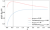 |
Fig. 4. Correlation between the mean residual χ presented in the bottom panel of Fig. 3 with |

To interpret the correlation between the residual of the reference model predictions and the simulations with  at the turnaround redshift, we recall that
  corresponds to the difference in the background expansion with respect to the static Λ-dominated expansion. For wDE < −1 (wDE > −1), the background expansion evolves faster (slower) than the standard model case. As a consequence, structure formation is slowed (accelerated), as gravitational instability has to counterbalance a stronger (weaker) DE repulsion. The turnaround is the moment when the two contributions, namely, cosmic expansion and gravitational instability, are in exact balance. In this sense, it is not surprising that the value of
  at the turnaround carries information on the effect of DE.
4.2. Halo mass function model
Equation (24) gives our final model for the multiplicity function. For ΛCDM, the parameters xΛ, i ∈ {a, p, q} evolve as described in Eqs.(13)–(17), r evolves as described in Eq. (27), and νp is assumed to be a free parameter that does not depend on cosmology.
The dynamical DE dependency for xi ∈ {a, p, q, r} is accounted for as follows

![$$ \begin{aligned}&= x_{\Lambda , i} \, \left\{ 1 + \frac{3\,\alpha _i}{2} \left[w_{\rm DE}(z_{\rm ta})+1\right]\,\Omega _{\rm DE}(z_{\rm ta})^{\beta _i} \right\} , \end{aligned} $$](/articles/aa/full_html/2025/05/aa53234-24/aa53234-24-eq50.gif)
where xΛ, i is the corresponding variable value for the ΛCDM model, while
is the turnaround redshift for a spherical top-hat perturbation that collapses at redshift z in an EdS cosmology.
4.3. Calibration
When running the first exploratory chains with all parameters free to vary, we detected that only a few parameters were statistically independent. To reduce the dimensionality of the model, we then decided to fix the pair of parameters that presented a correlation coefficient higher than 0.95. They are as follows:


Furthermore, all βi parameters were consistent with unity, and {αq, αr} is consistent with zero. With all these simplifications, our model has nine parameters that are free to vary {a1, a2, az, αa, p1, p2, q1, qz, σsys}. Their maximum-likelihood fit values and relative errors are presented in Table 4. In Fig. 5, we present the 68% and 95% percent contour level constraints of the parameters.
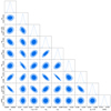 |
Fig. 5. Contour level constraints at 68% and 95% (dark and light shaded areas, respectively) on the nine free parameters describing the multiplicity function model and the systematic error. Dotted lines mark their values at the maximum likelihood estimate point (see Table 4). |
Maximum likelihood estimates and relative error for the multiplicity function and the systematic error parameters.
Notably, our model achieves a subpercent accuracy in the regime where we are not limited by shot noise, as the parameter controlling the systematic error σ is smaller than 1%. Therefore, our model complies with the calibration requirements for future surveys (see, for example, Salvati et al. 2020; Artis et al. 2021; Euclid Collaboration: Castro et al. 2023). Lastly, while our model extends the modeling of the HMF to dynamical DE, it contains the same number of degrees of freedom for the multiplicity function as its standard model version (Euclid Collaboration: Castro et al. 2023), that is, eight.
4.4. Model robustness
To assess our model’s robustness, we evaluated a p-value test using the validation set of the DUCA simulations. The p-value was computed by calculating the likelihood of the HMF extracted from the validation set, assuming our calibrated model. For each catalog, we generated 3 × 10⁵ random synthetic samples from the likelihood and computed p as the fraction of samples with a likelihood value as extreme as the real catalog. The results for all 20 simulations are shown in Fig. 6. To homogenize the distribution of likelihood values, we present the histogram for Δlnℒ, which is defined as the likelihood value minus the median of the likelihood value obtained from the synthetic samples. Each vertical line in Fig. 6 corresponds to one of the validation simulations and is color coded according to its S8 value. Lines lying near the histogram’s peak indicate a typical (i.e., likely) outcome under our model, whereas lines falling in the tails signify more extreme results. Thus, the position of a vertical line relative to the histogram reveals how well or poorly that particular simulation’s likelihood agrees with the distribution of synthetic realizations.
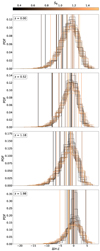 |
Fig. 6. Test p-value using the validation set of the DUCA simulations. For each catalog, we generated 3 × 10⁵ synthetic random samples from the likelihood and computed p as the fraction of samples with a likelihood value as extreme as the real catalog. The simulations have been color coded according to their S8 value. Each vertical line indicates the measured Δlnℒ for one of the validation simulations. |
Most catalogs show reasonable values for Δlnℒ that are distributed plausibly around the distribution peak. Two catalogs, one at z = 0.52 and one at z = 1.18, are noticeably different from the sample presenting extreme values for p. We selected these two simulations in order to scrutinize our model’s robustness, and they are presented in Fig. 7, where we show the model performance for different redshifts. The model on the left corresponds to the simulation with a low likelihood at z = 0.52. It has an extremely low value of S8 = 0.415, making Poisson noise much more evident in the residual plot in the bottom panel. Still, the model has a percent-level performance for the low-mass objects at low redshifts. More significant deviations appear at a higher redshift and mass, but the model is still consistent with the simulation within the error bars for most masses. Specifically for z = 0.52, we observed that the mass bins around a few times 1013 M⊙ h−1 count significantly more objects than the model. Excluding the two bins around this regime substantially improves the likelihood and the p-value. It is important to note that the original p-value for the catalog at this redshift was less than a 3 σ fluctuation. Therefore, it is likely that the relatively low performance of the model for this cosmology was just a statistical fluctuation.
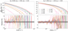 |
Fig. 7. Comparison between the HMF extracted from the two simulations with the lowest likelihood values (as shown in Fig. 6) and our model predictions. The left panel corresponds to the simulation with the lowest likelihood at redshift z = 0.52, and the right panel corresponds to the simulation with the lowest likelihood at z = 1.18. Different colors represent different redshifts. The simulation measurements are presented with Poisson error bars. |
The model on the right panel of Fig. 7 corresponds to the simulation with a low likelihood at z = 1.18. For this simulation, we observed that the model performance is at the subpercent level in the regime where we are not limited by Poisson noise. However, for the first mass bins at a low redshift, the simulation shows a few percent fewer objects than the model. Excluding these mass bins results in a much better likelihood and p-value. This case shows that the resolution correction proposed in Eq. (23) might have a residual cosmological dependency not captured by Eq. (23). This simulation has a high S8 = 1.402, so a more precise correction should likely consider the higher degree of non-linearity of this specific model. Improving the resolution effect modeling goes beyond the scope and needs of this paper.
Based on the results of this section, we conclude that our HMF model incorporating the effect of dynamical DE successfully passes extensive validation, robustly keeping its accuracy and precision level over an extended range for the choice of the relevant cosmological parameters beyond those sampled for the HMF calibration phase.
4.5. Comparison with other models
In Fig. 8, we depict a comparative analysis of the HMF at z = 0 showcasing to what degree our model aligns with or differs from established models in the literature. We show a comparison for two cosmological scenarios, one assuming cosmological parameters in agreement with Planck 2018 results (labeled Planck 18, see Aghanim et al. 2020) (solid curves) and one with the exact same values for all cosmological parameters but the DE equation of state w0 and wa, which we assume to be –0.8 and 0.5 (dashed curves). In the bottom panel of Fig. 8, we present the relative residual between the different models concerning our model. We considered the alternative models for the HMF from Euclid Collaboration: Castro et al. (2023), Tinker et al. (2008), Watson et al. (2013), Despali et al. (2016), Comparat et al. (2017), and Seppi et al. (2021), as they adopt the exact same definition for the SO threshold that we do. We used the models as implemented and made publicly available by Diemer (2018)15.
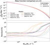 |
Fig. 8. Comparative analysis between our model’s prediction for the HMF at z = 0 and predictions by established models in the literature. The comparison is shown for two cosmological scenarios: one assuming cosmological parameters in agreement with Planck 2018 results and one with the same values for all cosmological parameters but w0 = −0.8 and wa = 0.5. The relative difference between the various models and our HMF calibration is shown in the bottom panel. |
We observed deviations in the residuals smaller than 10% in the regime 1013 ≲ M/M⊙ < 2 × 10¹⁵ for all models but Despali et al. (2016). The latter shows more significant deviations for M ≳ 4 × 10¹⁴ M⊙ h−1. Similar results have been reported in Euclid Collaboration: Castro et al. (2023). Notably, the impact of the chosen cosmological model is evident, as shown by the more pronounced spread in residuals when comparing results under the dynamic DE scenario. This highlights the lack of sensitivity of the other models to the DE equation of state. In contrast, our model proved that it is able to maintain its excellent performance in reproducing the predictions from simulations.
5. Conclusions
In this work, we have developed and calibrated a model for the HMF in the context of dynamical DE cosmologies while explicitly utilizing the w0waCDM framework, that is, using the CPL phenomenological parameterization of the DE equation of state (Chevallier & Polarski 2001; Linder 2003), as provided by Eq. (2). We extended our previous modeling presented in Euclid Collaboration: Castro et al. (2023) by including an additional degree of freedom to account for the evolving nature of DE. By leveraging the DUCA N-body cosmological simulations, which were carefully designed with a wide range of cosmological parameters, we assessed the impact of dynamical DE on the HMF and propose a new fitting function that effectively incorporates these effects.
We demonstrated that the dynamical DE component introduces a significant dependence on cosmology in the HMF parameters (see Fig. 3). This dependency is well captured by an enhanced parametrization of the multiplicity function. The parametrization introduces an additional dynamical degree of freedom through the value of the deceleration parameter  , defined in Eq. (28), at the epoch when a spherical top-hat perturbation, collapsing at a given time, reaches its turnaround (see Fig. 4).
We assessed the robustness of our model by using a validation set of 20 independent simulations spanning a wide range of cosmologies (see Fig. 6). The results consistently showed that our model maintains its subpercent accuracy across this set and is thus comparable to the residuals found for the calibration set. Despite minor deviations in a few extreme cosmologies, particularly those with very high or very low S8 values, which we presented in Fig. 7, the model proved effective, confirming that our new formulation is robust and broadly applicable to various cosmological models.
Furthermore, in Fig. 8, our comparative analysis demonstrated that existing HMF models introduced in the literature cannot accurately reproduce the effects of including dynamical DE. Our model, in contrast, consistently maintains its precision, effectively capturing the nuances introduced by the evolving DE equation of state. The validation and comparison results suggest that our model is well suited to enhancing the cosmological information carried by galaxy clusters identified in ongoing and upcoming multi-wavelength surveys.
Data availability
In Castro & Fumagalli (2024), we implement the new model presented in this paper16.
Publicly available at https://github.com/TiagoBsCastro/CCToolkit
Acknowledgments
It is a pleasure to thank Duca dos Anjos. We are grateful to thank Isabella Baccarelli, Fabio Pitari, and Caterina Caravita for their support with the CINECA environment. The DUCA simulations were run on the Leonardo-DCGP supercomputer as part of the Leonardo Early Access Program (LEAP). TC and SB are supported by the Agenzia Spaziale Italiana (ASI) under – Euclid-FASE D Attivita’ scientifica per la missione – Accordo attuativo ASI-INAF n. 2018-23-HH.0, by the PRIN 2022 PNRR project “Space-based cosmology with Euclid: the role of High-Performance Computing” (code no. P202259YAF), by the Italian Research Center on High-Performance Computing Big Data and Quantum Computing (ICSC), a project funded by European Union – NextGenerationEU – and National Recovery and Resilience Plan (NRRP) – Mission 4 Component 2, by the INFN INDARK PD51 grant, and by the National Recovery and Resilience Plan (NRRP), Mission 4, Component 2, Investment 1.1, Call for tender No. 1409 published on 14.9.2022 by the Italian Ministry of University and Research (MUR), funded by the European Union – NextGenerationEU – Project Title “Space-based cosmology with Euclid: the role of High-Performance Computing” – CUP J53D23019100001 – Grant Assignment Decree No. 962 adopted on 30/06/2023 by the Italian Ministry of Ministry of University and Research (MUR); We acknowledge the computing centre of CINECA and INAF, under the coordination of the “Accordo Quadro (MoU) per lo svolgimento di attivitá congiunta di ricerca Nuove frontiere in Astrofisica: HPC e Data Exploration di nuova generazione”, for the availability of computing resources and support. We acknowledge the use of the HOTCAT computing infrastructure of the Astronomical Observatory of Trieste – National Institute for Astrophysics (INAF, Italy) (see Bertocco et al. 2020; Taffoni et al. 2020).
References
- Adamek, J., Angulo, R. E., Arnold, C., et al. 2023, JCAP, 06, 035 [NASA ADS] [Google Scholar]
- Aghanim, N., Akrami, Y., Ashdown, M., et al. 2020, A&A, 641, A6 [Erratum: A&A 652, C4 (2021)] [NASA ADS] [CrossRef] [EDP Sciences] [Google Scholar]
- Allen, S. W., Evrard, A. E., & Mantz, A. B. 2011, ARA&A, 49, 409 [Google Scholar]
- Angulo, R. E., & Hahn, O. 2022, Liv. Rev. Comput. Astrophys., 8, 1 [CrossRef] [Google Scholar]
- Angulo, R. E., & Pontzen, A. 2016, MNRAS, 462, L1 [NASA ADS] [CrossRef] [Google Scholar]
- Angulo, R. E., & White, S. D. M. 2010, MNRAS, 401, 1796 [NASA ADS] [CrossRef] [Google Scholar]
- Aricò, G., Angulo, R. E., Contreras, S., et al. 2021, MNRAS, 506, 4070 [CrossRef] [Google Scholar]
- Artis, E., Melin, J.-B., Bartlett, J. G., & Murray, C. 2021, A&A, 649, A47 [NASA ADS] [CrossRef] [EDP Sciences] [Google Scholar]
- Batista, R. C. 2021, Universe, 8, 22 [Google Scholar]
- Behroozi, P. S., Wechsler, R. H., & Wu, H.-Y. 2013a, ApJ, 762, 109 [NASA ADS] [CrossRef] [Google Scholar]
- Behroozi, P. S., Wechsler, R. H., Wu, H.-Y., et al. 2013b, ApJ, 763, 18 [NASA ADS] [CrossRef] [Google Scholar]
- Benson, B. A., et al. 2014, Proc. SPIE Int. Soc. Opt. Eng., 9153, 91531P [Google Scholar]
- Bertocco, S., Goz, D., Tornatore, L., et al. 2020, in Astronomical Data Analysis Software and Systems XXIX, Astronomical Society of the Pacific Conference Series, 527, 303 [NASA ADS] [Google Scholar]
- Bhattacharya, S., Heitmann, K., White, M., et al. 2011, ApJ, 732, 122 [NASA ADS] [CrossRef] [Google Scholar]
- Bocquet, S., Saro, A., Dolag, K., & Mohr, J. J. 2016, MNRAS, 456, 2361 [Google Scholar]
- Bocquet, S., Dietrich, J. P., Schrabback, T., et al. 2019, ApJ, 878, 55 [Google Scholar]
- Bocquet, S., Heitmann, K., Habib, S., et al. 2020, ApJ, 901, 5 [Google Scholar]
- Bond, J. R., Cole, S., Efstathiou, G., & Kaiser, N. 1991, ApJ, 379, 440 [NASA ADS] [CrossRef] [Google Scholar]
- Borgani, S., Rosati, P., Tozzi, P., et al. 2001, ApJ, 561, 13 [NASA ADS] [CrossRef] [Google Scholar]
- Bryan, G. L., & Norman, M. L. 1998, ApJ, 495, 80 [NASA ADS] [CrossRef] [Google Scholar]
- Castorina, E., Sefusatti, E., Sheth, R. K., Villaescusa-Navarro, F., & Viel, M. 2014, JCAP, 02, 049 [CrossRef] [Google Scholar]
- Castro, T., & Fumagalli, A. 2024, https://doi.org/10.5281/zenodo.13479345 [Google Scholar]
- Castro, T., Borgani, S., Dolag, K., et al. 2020, MNRAS, 500, 2316 [Google Scholar]
- Chevallier, M., & Polarski, D. 2001, Int. J. Mod. Phys. D, 10, 213 [Google Scholar]
- Comparat, J., Prada, F., Yepes, G., & Klypin, A. 2017, MNRAS, 469, 4157 [Erratum: MNRAS 483, 2561–2562 (2019)] [NASA ADS] [CrossRef] [Google Scholar]
- Cooray, A., & Sheth, R. K. 2002, Phys. Rept., 372, 1 [Google Scholar]
- Copeland, E. J., Sami, M., & Tsujikawa, S. 2006, Int. J. Mod. Phys. D, 15, 1753 [NASA ADS] [CrossRef] [Google Scholar]
- Costanzi, M., Villaescusa-Navarro, F., Viel, M., et al. 2013, JCAP, 12, 012 [Google Scholar]
- Costanzi, M., Saro, A., Bocquet, S., et al. 2021, PRD, 103, 043522 [NASA ADS] [CrossRef] [Google Scholar]
- Courtin, J., Rasera, Y., Alimi, J. M., et al. 2011, MNRAS, 410, 1911 [NASA ADS] [Google Scholar]
- Crocce, M., Fosalba, P., Castander, F. J., & Gaztanaga, E. 2010, MNRAS, 403, 1353 [NASA ADS] [CrossRef] [Google Scholar]
- Cui, W., Baldi, M., & Borgani, S. 2012, MNRAS, 424, 993 [NASA ADS] [CrossRef] [Google Scholar]
- Cui, W., Borgani, S., & Murante, G. 2014, MNRAS, 441, 1769 [NASA ADS] [CrossRef] [Google Scholar]
- Dakin, J., Hannestad, S., Tram, T., Knabenhans, M., & Stadel, J. 2019a, JCAP, 08, 013 [Google Scholar]
- Dakin, J., Brandbyge, J., Hannestad, S., Haugbølle, T., & Tram, T. 2019b, JCAP, 02, 052 [Google Scholar]
- Dakin, J., Hannestad, S., & Tram, T. 2022, MNRAS, 513, 991 [CrossRef] [Google Scholar]
- DESI Collaboration (Aghamousa, A., et al.) 2016, arXiv e-prints [arXiv:1611.00036] [Google Scholar]
- Despali, G., Giocoli, C., Angulo, R. E., et al. 2016, MNRAS, 456, 2486 [NASA ADS] [CrossRef] [Google Scholar]
- Diemer, B. 2018, ApJS, 239, 35 [NASA ADS] [CrossRef] [Google Scholar]
- Diemer, B. 2020, ApJ, 903, 87 [NASA ADS] [CrossRef] [Google Scholar]
- Eke, V. R., Cole, S., & Frenk, C. S. 1996, MNRAS, 282, 263 [CrossRef] [Google Scholar]
- Euclid Collaboration (Castro, T., et al.) 2023, A&A, 671, A100 [CrossRef] [EDP Sciences] [Google Scholar]
- Euclid Collaboration (Castro, T., et al.) 2024a, A&A, 685, A109 [NASA ADS] [CrossRef] [EDP Sciences] [Google Scholar]
- Euclid Collaboration (Castro, T., et al.) 2024b, A&A, 691, A62 [Google Scholar]
- Euclid Collaboration (Mellier, Y., et al.) 2025, A&A, 697, A1 [Google Scholar]
- Foreman-Mackey, D., Hogg, D. W., Lang, D., & Goodman, J. 2013, PASJ, 125, 306 [Google Scholar]
- Frieman, J., Turner, M., & Huterer, D. 2008, ARA&A, 46, 385 [NASA ADS] [CrossRef] [Google Scholar]
- Fumagalli, A., Costanzi, M., Saro, A., Castro, T., & Borgani, S. 2024, A&A, 682, A148 [NASA ADS] [CrossRef] [EDP Sciences] [Google Scholar]
- Kitayama, T., & Suto, Y. 1996, ApJ, 469, 480 [CrossRef] [Google Scholar]
- Kravtsov, A. V., & Borgani, S. 2012, ARA&A, 50, 353 [Google Scholar]
- Lesgourgues, J., & Pastor, S. 2006, Phys. Rept., 429, 307 [NASA ADS] [CrossRef] [Google Scholar]
- Linder, E. V. 2003, Phys. Rev. Lett., 90, 091301 [Google Scholar]
- LSST Science Collaborations (Abell, P. A., et al.) 2009, arXiv e-prints [arXiv:0912.0201] [Google Scholar]
- Maartens, R., Abdalla, F. B., Jarvis, M., & Santos, M. G. 2015, PoS, AASKA14, 016 [Google Scholar]
- Majumdar, S., & Mohr, J. J. 2004, ApJ, 613, 41 [NASA ADS] [CrossRef] [Google Scholar]
- Marulli, F., Veropalumbo, A., Sereno, M., et al. 2018, A&A, 620, A1 [NASA ADS] [CrossRef] [EDP Sciences] [Google Scholar]
- Ondaro-Mallea, L., Angulo, R. E., Zennaro, M., Contreras, S., & Aricò, G. 2021, MNRAS, 509, 6077 [NASA ADS] [CrossRef] [Google Scholar]
- Pace, F., Meyer, S., & Bartelmann, M. 2017, JCAP, 10, 040 [Google Scholar]
- Peebles, P. J. E. 2020, The large-scale structure of the universe (Princeton university press), 98 [Google Scholar]
- Peebles, P. J. E., & Ratra, B. 2003, Rev. Mod. Phys., 75, 559 [NASA ADS] [CrossRef] [Google Scholar]
- Planck Collaboration XXIV. 2016, A&A, 594, A24 [NASA ADS] [CrossRef] [EDP Sciences] [Google Scholar]
- Predehl, P., Andritschke, R., Arefiev, V., et al. 2021, A&A, 647, A1 [EDP Sciences] [Google Scholar]
- Press, W. H., & Schechter, P. 1974, ApJ, 187, 425 [Google Scholar]
- Sáez-Casares, I., Rasera, Y., Richardson, T. R. G., & Corasaniti, P. S. 2024, A&A, 691, A323 [NASA ADS] [CrossRef] [EDP Sciences] [Google Scholar]
- Salvati, L., Douspis, M., & Aghanim, N. 2020, A&A, 643, A20 [NASA ADS] [CrossRef] [EDP Sciences] [Google Scholar]
- Schneider, A., & Teyssier, R. 2015, JCAP, 12, 049 [Google Scholar]
- Schuecker, P., Bohringer, H., Collins, C. A., & Guzzo, L. 2003, A&A, 398, 867 [NASA ADS] [CrossRef] [EDP Sciences] [Google Scholar]
- Seppi, R., Comparat, J., Nandra, K., et al. 2021, A&A, 652, A155 [NASA ADS] [CrossRef] [EDP Sciences] [Google Scholar]
- Shen, D., Kokron, N., DeRose, J., et al. 2025, JCAP, 03, 056 [Google Scholar]
- Sheth, R. K., & Tormen, G. 1999, MNRAS, 308, 119 [Google Scholar]
- Sheth, R. K., Mo, H. J., & Tormen, G. 2001, MNRAS, 323, 1 [NASA ADS] [CrossRef] [Google Scholar]
- Spergel, D., Gehrels, N., Baltay, C., et al. 2015, arXiv e-prints [arXiv:1503.03757] [Google Scholar]
- Taffoni, G., Becciani, U., Garilli, B., et al. 2020, in Astronomical Data Analysis Software and Systems XXIX, Astronomical Society of the Pacific Conference Series, 527, 307 [NASA ADS] [Google Scholar]
- Tinker, J. L., Kravtsov, A. V., Klypin, A., et al. 2008, ApJ, 688, 709 [NASA ADS] [CrossRef] [Google Scholar]
- Tsallis, C. 1988, J. Stat. Phys., 52, 479 [NASA ADS] [CrossRef] [Google Scholar]
- Tsallis, C., & Stariolo, D. A. 1996, Phys. A: Stat. Mech. Appl., 233, 395 [Google Scholar]
- Vagnozzi, S., Brinckmann, T., Archidiacono, M., et al. 2018, JCAP, 09, 001 [NASA ADS] [Google Scholar]
- Velliscig, M., van Daalen, M. P., Schaye, J., et al. 2014, MNRAS, 442, 2641 [Google Scholar]
- Vikhlinin, A., Kravtsov, A. V., Burenin, R. A., et al. 2009, ApJ, 692, 1060 [Google Scholar]
- Virtanen, P., Gommers, T., Oliphant, T. E., et al. 2020, Nat. Methods, 17, 261 [NASA ADS] [CrossRef] [Google Scholar]
- Watson, W. A., Iliev, I. T., D’Aloisio, A., et al. 2013, MNRAS, 433, 1230 [Google Scholar]
- Weinberg, S. 2008, Cosmology (Oxford University Press) [Google Scholar]
- Weinberg, D. H., Mortonson, M. J., Eisenstein, D. J., et al. 2013, Phys. Rept., 530, 87 [NASA ADS] [CrossRef] [Google Scholar]
- Xiang, Y., & Gong, X. G. 2000, Phys. Rev. E, 62, 4473 [NASA ADS] [CrossRef] [Google Scholar]
- Xiang, Y., Sun, D. Y., Fan, W., & Gong, X. G. 1997, Phys. Lett. A, 233, 216 [NASA ADS] [CrossRef] [Google Scholar]
All Tables
Force parameters used in the DUCA set of simulations, including short-range and long-range force specifications.
Maximum likelihood estimates and relative error for the multiplicity function and the systematic error parameters.
All Figures
|
Fig. 1. Cosmological parameters for the three subsets of the DUCA simulations (see Sect. 3.1 for details). |
| In the text | |
|
Fig. 2. Relative difference of the HMF extracted from the primary set to their high-resolution counterpart. We have labeled the cosmologies from the extended set according to their value of S8. The results are shown as a function of the number of particles Np in the primary simulation. |
| In the text | |
|
Fig. 3. Top: Comparison between the HMF predicted by the model of Euclid Collaboration: Castro et al. (2023) (curves) and the HMF measured for the extended large simulations (points). Error bars associated with each simulation point correspond to the Poisson uncertainty. Bottom: Relative difference between the model and the simulations. Different panels indicate different redshifts; from left to right, z = 0.00, 1.18, and 1.98. |
| In the text | |
|
Fig. 4. Correlation between the mean residual χ presented in the bottom panel of Fig. 3 with |
| In the text | |
|
Fig. 5. Contour level constraints at 68% and 95% (dark and light shaded areas, respectively) on the nine free parameters describing the multiplicity function model and the systematic error. Dotted lines mark their values at the maximum likelihood estimate point (see Table 4). |
| In the text | |
|
Fig. 6. Test p-value using the validation set of the DUCA simulations. For each catalog, we generated 3 × 10⁵ synthetic random samples from the likelihood and computed p as the fraction of samples with a likelihood value as extreme as the real catalog. The simulations have been color coded according to their S8 value. Each vertical line indicates the measured Δlnℒ for one of the validation simulations. |
| In the text | |
|
Fig. 7. Comparison between the HMF extracted from the two simulations with the lowest likelihood values (as shown in Fig. 6) and our model predictions. The left panel corresponds to the simulation with the lowest likelihood at redshift z = 0.52, and the right panel corresponds to the simulation with the lowest likelihood at z = 1.18. Different colors represent different redshifts. The simulation measurements are presented with Poisson error bars. |
| In the text | |
|
Fig. 8. Comparative analysis between our model’s prediction for the HMF at z = 0 and predictions by established models in the literature. The comparison is shown for two cosmological scenarios: one assuming cosmological parameters in agreement with Planck 2018 results and one with the same values for all cosmological parameters but w0 = −0.8 and wa = 0.5. The relative difference between the various models and our HMF calibration is shown in the bottom panel. |
| In the text | |
Current usage metrics show cumulative count of Article Views (full-text article views including HTML views, PDF and ePub downloads, according to the available data) and Abstracts Views on Vision4Press platform.
Data correspond to usage on the plateform after 2015. The current usage metrics is available 48-96 hours after online publication and is updated daily on week days.
Initial download of the metrics may take a while.