| Issue |
A&A
Volume 697, May 2025
|
|
|---|---|---|
| Article Number | A152 | |
| Number of page(s) | 19 | |
| Section | Stellar structure and evolution | |
| DOI | https://doi.org/10.1051/0004-6361/202452360 | |
| Published online | 14 May 2025 | |
Variability of Galactic blue supergiants observed with TESS
1
Astronomical Institute, Czech Academy of Sciences, Fričova 298, 251 65 Ondřejov, Czech Republic
2
Instituto de Astrofísica La Plata, CCT La Plata, CONICET-UNLP, Paseo del Bosque S/N, B1900FWA La Plata, Argentina
3
Departamento de Espectroscopía, Facultad de Ciencias Astronómicas y Geofísicas, Universidad Nacional de La Plata (UNLP), Paseo del Bosque S/N, B1900FWA, La Plata, Argentina
⋆ Corresponding author: This email address is being protected from spambots. You need JavaScript enabled to view it.
Received:
24
September
2024
Accepted:
26
March
2025
Abstract
Context. Blue supergiants (BSGs) span phases between the main sequence and the late stages of massive stars, which makes them valuable for assessing the physics that drives stars across diverse evolutionary channels.
Aims. By exploring correlations between the parameters of BSGs and their variability properties, we aim to improve the constraints on models of the evolved star structure and on the physics of post-main-sequence evolution.
Methods. We conducted a variability study of 41 BSGs with known spectroscopic parameters in the Galaxy using high-precision photometry from the Transiting Exoplanet Survey Satellite. Stellar luminosities were calculated from the fit of multiband photometry and using the latest distance estimates from Gaia. We described the time domain of the stars by means of three statistical measures and extracted prominent frequencies via an iterative pre-whitening process. We also investigated the debated stochastic low-frequency (SLF) variability, which manifests itself in all amplitude spectra.
Results. We report a positive correlation between the amplitude of photometric variability and the stellar luminosity. For log (L/L⊙) ≲ 5, stars display frequencies that match the rotational one, suggesting that variability is driven by surface spots and/or features embedded in the wind. For log (L/L⊙) ≳ 5, variables of the α Cygni class manifest themselves via their diverse and/or time-variant photometric properties and their systematically lower frequencies. Moreover, we report a positive correlation between the SLF variability amplitude and the effective temperature, which indicates that the stellar age plays an influential role in the emergence of the background signal beyond the main sequence. A positive, though weak, correlation is also observed between the intrinsic brightness and the SLF variability amplitude, similar to the findings in the Large Magellanic Cloud, which suggests an excitation mechanism that depends only mildly on metallicity. Exceptionally, the α Cygni variables display a suppressed SLF variability that points to the interior changes that the evolving stars undergo.
Key words: stars: evolution / stars: massive / stars: oscillations / stars: rotation / stars: variables: general
© The Authors 2025
 Open Access article, published by EDP Sciences, under the terms of the Creative Commons Attribution License (https://creativecommons.org/licenses/by/4.0), which permits unrestricted use, distribution, and reproduction in any medium, provided the original work is properly cited.
This article is published in open access under the Subscribe to Open model. This email address is being protected from spambots. You need JavaScript enabled to view it. to support open access publication.
1. Introduction
As some of the brightest stars in galaxies and young star associations, the blue supergiants (BSGs) provide us information on the key parameters of their host environments, such as age, kinematics, metallicity, and distance (Bresolin et al. 2006; Urbaneja et al. 2008; Kudritzki et al. 2012). Their accessibility enables studies to be undertaken with high resolution, and on a systematic basis, providing the means to describe mechanisms that are pivotal to the evolution of massive stars.
The high number of reported BSGs (Castro et al. 2014; de Burgos et al. 2023) contradicts the scarcity predicted by the standard single-star evolutionary theory (Bellinger et al. 2024), which is referred to as the BSG problem. To resolve this discrepancy, several scenarios for creating BSGs in addition to the classical post-main-sequence objects have been proposed, namely post-mass-transfer stars (Farrell et al. 2019), stripped-envelope stars (Klencki et al. 2022), binary mergers (Henneco et al. 2024; Menon et al. 2024), and stars that experience an extended main-sequence phase due to possessing enlarged convective cores (Brott et al. 2011; Martinet et al. 2021) or due to being subject to enhanced rotationally induced mixing (de Mink et al. 2013). In this respect, the key to assessing the nature of BSGs and interpreting their statistics is a thorough understanding of their interior, their mass loss, and the interplay between binary components.
Further contributing to the puzzling demographics of BSGs, several members of the class are believed to have already passed through the red supergiant (RSG) phase and are now captured at late stages (Meynet et al. 2015). These so-called post-RSGs have experienced significant loss of their hydrogen envelope, exposing material from the interior to the surface and surroundings. Spectroscopic tracers of this processed material provide a means to identify the evolved status of several of these objects (e.g., Kraus et al. 2023), although other post-RSGs cease to show abnormal chemistry (Georgy et al. 2014) or a gaseous and/or dusty circumstellar environment (Oudmaijer et al. 2009). The interior of post-RSGs is subject to nonadiabatic processes (Saio et al. 2013; Glatzel & Kraus 2024), which are linked to the as yet poorly understood strange-mode instabilities. These have been proposed to be responsible for the launch of episodic mass loss and might lead to a buildup of circumstellar envelopes (Aerts et al. 2010). They also require that the stars have experienced copious amounts of mass loss in a short time, during their prior RSG phase (Saio et al. 2013; Georgy et al. 2014; Glatzel & Kraus 2024). Moreover, post-RSG BSGs display semi-regular variability and periods of few days to several tens of days, which are attributed to opacity-driven oscillations (Kaufer et al. 1997; Lefever et al. 2007). These objects are known as α Cygni variables, following the name of the prototype BSG star.
The stellar variability integrates the feedback from the different processes that take place in the interior and atmosphere, serving as a potent indicator of the structural changes that stars undergo at different stages of evolution. From the interior of BSGs, the most commonly studied sources of (quasi-)periodic and stochastic signals include p- and g-modes that are driven by the κ mechanism operating in the metal opacity bump (e.g., Saio et al. 2006; Lefever et al. 2007), low-frequency waves that are generated by sub-photospheric convection (Cantiello et al. 2009), and internal gravity waves (IGWs; Bowman et al. 2019a, 2020). As soon as the waves reach the surface, they manifest as coherent or stochastic fluctuations in the brightness and as variability in the line profiles (e.g., Kaufer et al. 2006; Simón-Díaz et al. 2018). Moreover, pulsations are believed to contribute to line broadening through the effect of macroturbulence (Aerts et al. 2009; Simón-Díaz et al. 2010; Aerts et al. 2018; Bowman et al. 2020). Outside the interior, rotational modulation is another source of periodic signal that is generated by spots in the surface and/or corotating inhomogeneities in the wind (Aerts et al. 2013, 2018). Evidence of the deep interior dynamics propagating into the wind has been demonstrated (Kraus et al. 2015; Haucke et al. 2018; Aerts et al. 2017; Cidale et al. 2023), implying an auxiliary role for the pulsations in contributing to the line-driven mass loss. Finally, stellar encounters introduce variability in the case of eclipsing and/or spectroscopic systems, and via evidence in the frequency spectra of mixed or tidally induced modes (Degroote et al. 2012; Southworth et al. 2020).
Probably the most debated type of variability in the frequency spectra of early-type stars is the stochastic low-frequency (SLF) variability. Its first detection in three O-type stars by Blomme et al. (2011) was followed by systematic analyses of extended OB-star samples that confirmed the ubiquity of the signal (Bowman et al. 2019b,a, 2020; Burssens et al. 2020; Ma et al. 2024; Shen et al. 2024). Hydrodynamical simulations of core convection and wave propagation have been able to reproduce the observed SLF variability, assigning its origin to IGWs that are excited at the interface between the convective core and the radiative envelope (Rogers et al. 2013; Edelmann et al. 2019; Ratnasingam et al. 2023). Other studies, on the other hand, have demonstrated that core-excited IGWs are unlikely to generate variability consistent with the observations (Lecoanet et al. 2019; Anders et al. 2023); a thoroughly discussed alternative to the core-convection scenario is the turbulent motion in the subsurface convection zones of the stellar envelope (Cantiello et al. 2021; Schultz et al. 2022). This excitation mechanism alone, however, is considered to not apply to stars in low-metallicity environments where this form of variability is observed to persist (Bowman et al. 2024), or to stars on the main sequence that presumably lack subsurface convection zones (e.g., Jermyn et al. 2022). Recent findings suggest that both core and near-surface convection could shape the stochastic signal over different ranges of frequencies in the power spectra of the stars (Thompson et al. 2024), though the possibility that the inductive role of the two mechanisms depends on the stellar age and metallicity is also under consideration (Bowman et al. 2024). As the discussion of the source of the enigmatic signal continues, refining our knowledge of its underlying physics has important implications for the modeling of stellar evolution, due to the role of the propagating waves in driving the angular momentum transport, rotation, and mixing in the interior of the stars (Rogers et al. 2013; Aerts et al. 2019; Bowman 2020).
The signatures of the ambiguous processes that govern the nature of BSGs are imprinted into their variability profile. Applying advanced methodology for the exploration of the frequency domain has been shown to be effective for identifying different oscillation modes, constraining parameters of the core, and even differentiating between the distinct evolutionary scenarios (Degroote et al. 2010; Bowman et al. 2019a; Bowman 2020; Burssens et al. 2023; Bellinger et al. 2024; Henneco et al. 2024). A particular breakthrough in asteroseismology has been achieved since the launch of NASA’s Transiting Exoplanet Survey Satellite (TESS; Ricker et al. 2015). The mission holds a major advantage over its predecessor monitoring surveys thanks to its all-sky coverage, which enables systematic studies to be undertaken and statistical inferences to be drawn over stellar ensembles. Such ensembles include massive stars in both early (e.g., Pedersen et al. 2019; Burssens et al. 2020; Krtička & Feldmeier 2021; Gebruers et al. 2022; Labadie-Bartz et al. 2022) and evolved (or transition) phases (Nazé et al. 2021; Dorn-Wallenstein et al. 2019, 2022; Spejcher et al. 2025). These works have been mapping the different manifestations as a function of the stellar parameters, collectively improving our understanding of stellar structure and evolution.
Along the same line, we present a variability study based on TESS data of southern Galactic BSGs. We explore associations between their well-determined parameters and the features of the time and frequency domain. Particular attention is paid on the reported α Cygni variables of the sample, and we probe them for signatures of their evolved status in the variability statistics. Additionally, we model the SLF variability of the stars and compare its parameters to those from the study of BSGs in the Large Magellanic Cloud (LMC; Bowman et al. 2019a). With the metallicity constrained, we aim to narrow down the possible scenarios explaining the ambiguous origin of the signal.
In Sect. 2 we present our sample of BSGs and the processing of their TESS data, in Sect. 3 we describe the process for extracting the frequencies from the multi-period signals and introduce the metrics for describing the time domain, and in Sect. 4 we fit the spectral energy distributions (SEDs), which enables us to assess the stellar luminosities. We discuss the results of the study in Sect. 5 and provide concluding remarks in Sect. 6.
2. Sample selection and TESS photometry
2.1. Source catalog
Our explored sample is taken from the catalog of Fraser et al. (2010), which consists of Galactic B−type supergiants observed in 2004 − 2005 with the Fiber-fed Extended Range Optical Spectrograph (FEROS; Kaufer et al. 1999), a high-resolution spectrograph (R ∼ 48 000) installed on the 2.2-m Max Planck Institute (MPI) telescope, at the European Southern Observatory (ESO), La Silla, Chile. The stellar parameters were extracted by fitting the observations with theoretical models, which were generated using the nonlocal thermodynamic equilibrium code TLUSTY (Hubeny & Lanz 1995). The uncertainties in the log g and log Teff measurements were reported as ±0.1 dex and ±0.02 dex, respectively.
2.2. TESS time-series data
Launched in 2018, TESS (Ricker et al. 2015) has been conducting monitoring of 85% of the sky with an angular resolution of 21″/pixel, using a wide red/optical passband that spans the wavelength range 600 − 1000 nm. The field of view of TESS covers a sky area of 24° ×96° (known as sector), which is observed for two spacecraft orbits, or ∼27 days.
We performed cross-matching between the source catalog and the TESS database, removing stars that are not observed by TESS as well as those with poor-quality data (e.g., stars captured at the edge of the detector) that were unsuitable for further investigation. In addition, we excluded stars from the source catalog that are brighter than the TESS magnitude (T) limit of 4 mag, a value that has been tested for the ability of the TESS CCD detectors to conserve charge from bright sources (Vanderspek et al. 2018). Our studied sample consists of 41 BSGs, which we present in Table A.1, along with their coordinates and spectral classifications from SIMBAD, their TESS Input Catalog (TIC) number, T, and observed sectors.
For the systematic analysis of the time-series data, we used the lightkurve software package (Lightkurve Collaboration 2018). Two types of flux were explored; preprocessed and own extracted and systematics-corrected one.
2.2.1. PDCSAP flux
Using the lightkurve.search_lightcurve routine and the TIC identification number of the objects, we queried the Mikulski Archive for Space Telescopes1 (MAST) for light curves that have been processed with the dedicated pipeline for the survey (Science Processing Operations Center; SPOC). The light curve files contain data that were taken with a 2-min cadence, and which have been corrected for the systematic trends using the co-trending basis vectors method (photometry flagged as PDCSAP_FLUX; Pre-search Data Conditioning Simple Aperture Photometry). The provided data come along with the pixel mask (“optimal” aperture) that has been produced by the pipeline for the extraction of the photometric signal.
2.2.2. Full-frame images
As an adjunct to the study of the preprocessed flux, we explored cutouts from the full-frame images, so-called target pixel files (TPFs), using the TESScut service (Brasseur et al. 2019). The process was performed with the lightkurve.search_tesscut routine and setting the cutout length to 20 × 20 pixels, which was enough to encompass the entirety of the target flux and sufficient background signal, for all sample stars.
We superimposed photometric sources from the Gaia Data Release 3 (DR3; Gaia Collaboration 2022) database on the TPFs, and located the target star. We then overlaid the SPOC aperture and searched, sector by sector, for cases where adjustment of the aperture was desirable in order to minimize biases related to under- or over-collecting signal. In such an event, we defined a custom mask for manual extraction of the target flux; starting from the pixel containing the Gaia target source, we extended the aperture vertically (across the rows) in both directions of the charge blooming, for as long as the ratio of the flux to that of the target pixel remained higher than a threshold value. The process was repeated sideways for the adjacent columns. The threshold was evaluated empirically to include adequate signal of the studied star without excess contribution from the background; it was set to 0.15 for most of the sample stars, and reached down to 0.07. For three stars proximal to a bright source (see Sect. 2.2.3), we increased this value up to 0.25. Next, the extracted light curves were corrected against the instrumental noise and the systematics using the lightkurve.RegressionCorrector class. For this process, we defined as background pixels those fainter than a modest threshold (10−4σ) below the median flux of the TPF. The dimensionality of the background vector space was reduced using principal component analysis, and linear regression was performed to detrend the science data.
The processed data of each above types of fluxes were fit with a low-order polynomial and were detrended. We converted the normalized flux Fn to magnitudes using the formula
 (1)
(1)
The time series of consecutive sectors with the same cadence were then joined into a larger observing window in order to increase the resolution of our frequency analysis and accuracy of time-domain statistics. We display the light curves of selected BSGs in Fig. 1, and those of the entire sample in the external appendix available on Zenodo.
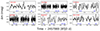 |
Fig. 1. Time-series photometry from TESS of selected BSGs. Data are detrended, normalized, and converted into units of magnitude. For each star, we show data from different sectors over multiple panels. Consecutive sectors are joined together, and their numbers are displayed at the bottom of each panel. |
2.2.3. Contamination in the TESS aperture
The main drawback of TESS is the low spatial resolution, which makes densely populated areas in the sky prone to contamination effects. The degree of contamination for a TESS source can be assessed from the ratio of the light that comes from the target to the total light that is captured within the aperture. This metric is calculated by SPOC and is stored in the header of the light curve files under the keyword CROWDSAP. In cases where a custom (adjusted) mask was selected for extracting the signal from the TPFs (Sect. 2.2.2), we (re)assessed the metric as
 (2)
(2)
where f* and fk are the fluxes from the target and the k-th source contained in the aperture (including the target), respectively, which were calculated from the TESS magnitudes (Paegert et al. 2021). A comparison between CROWDSAP and the adjusted values yielded minor differences of ≲0.01; greater differences were only found for the stars HD 111973 and HD 152234.
We provide the contamination metric of the stars in Table A.1. Values close to 1 indicate that the flux from all secondary sources in the aperture contributes minimally to the target light curve, whereas the photometry becomes less reliable for values of the metric ≲0.8 (Guerrero et al. 2021). The latter case concerns stars HD 152234 and HD 111973. These are followed by HD 141318 and HD 79186, with CROWDSAP+ values 0.84 and 0.89, respectively. The rest of the sample displays CROWDSAP+ > 0.9, with the vast majority of these stars exceeding 0.95.
Finally, during the inspection of the TPFs (Sect. 2.2.2) we flagged three stars, which could be affected by flux from a bright source that is located outside the photometric aperture. These objects are the above mentioned HD 111973 and HD 79186, as well as HD 94493.
2.3. Overlapping TESS studies and reported variables
We checked in TESS studies for overlapping cases and report HD 51309 to have been studied by Burssens et al. (2020) and Bowman et al. (2020) with data from Sectors 1 − 13. We extend here the variability study to Sector 33 and complement with the time-domain features of the star, measuring also its luminosity from the modeling of multiband photometry.
During a combined cross-matching of our stars with the General Catalog of Variable Stars (GCVS; Samus et al. 2017) and the variability study with HIPPARCOS by Lefèvre et al. (2009), nine stars of the sample were identified as α Cygni variables2. Moreover, three BSGs are reported in SIMBAD as double or multiple systems: HD 152234 and HD 111973 (which are discussed above for their crowding effect) and HD 77581. HD 77581 is located in the well-studied high-mass X-ray system Vela X-1.
3. Methodology
The TESS data of the Galactic BSGs display variability of up to ∼0.1 mag in amplitude, which is described as (quasi-)periodic with dominant frequencies that, for several stars, vary across the different observing windows. We identify cases where variability displays irregular patterns that can be also explained as a superposition of cycles with different periods. At a first glance, the signal of several stars with low photometric amplitude resembles that of instrumental noise (the least luminous BSGs; see Sect. 5), and which typically characterizes the sky objects as “invariant.”
3.1. Extraction of frequencies
To explore the presence of periodic signals in the TESS data, we made use of the lightkurve.Periodogram class and computed the Lomb-Scargle periodograms (amplitude spectra). We extracted the prominent frequencies via an iterative pre-whitening process; at each iteration, we selected the frequency with the highest amplitude, fit the light curve with the corresponding sinusoidal model and subtracted it. The residuals of the fit were then subjected to a new iteration for identifying the next peak frequency, and the process was repeated until a termination criterion was met (see Sect. 3.2). The procedure is demonstrated in Fig. 2 for star HD 94493 using the stitched light curves from Sectors 63 and 64.
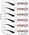 |
Fig. 2. Iterative pre-whitening for the extraction of frequencies for HD 94493 (Sectors 63 and 64). Left: Calculated amplitude spectra (Lomb-Scargle periodograms) shown in logarithmic scale. A vertical line at the top of each panel points toward the extracted frequency, which is reported in the lower left. Right: Light curve of the star (black points) with the integrated fit model of sinusoidals superimposed (red). |
The frequencies that were extracted from an observing window were categorized into four types using the Rayleigh resolution 1/ΔT, where ΔT is the length of the studied time span. These types are:
-
Independent frequencies, fi. These are significant peaks that are typically identified early in the extraction process and are physically interpreted in BSGs either as opacity-driven g- and/or p-modes or as the rotational modulation by an aspherical wind and/or surface spots.
-
Harmonic frequencies, which were identified as integer multiples of the independent ones.
-
Combinations (algebraic sums) of two previously extracted frequencies.
-
Frequencies that were repeated within the adopted resolution. These are likely to be spurious detections that emerge during the subtraction of the periodic model, and essentially trace the removed signal. The probability of them being unresolved mode orders of period-spacing patterns (and thus having a physical origin) is too considered.
In addition, we considered frequencies higher than 0.07 d−1 to be credible in order to resolve a minimum of two cycles per sector. Joining consecutive sectors to form a larger observing window did not lift this constraint, given that the data of the separate sectors were individually normalized, potentially washing out periods longer than ∼14 days. The total of the independent frequencies and their parameters, subject of our investigation in Sect. 5, are tabulated in Appendix B.
We explored whether the identified frequencies are associated with effects introduced by the stellar rotation, in a similar manner as in Burssens et al. (2020). We calculated the lowest frequency expected from the reported υ sin i values from Fraser et al. (2010) and our inferred radii (see Sect. 4),
![Mathematical equation: $$ \begin{aligned} \nu _{\rm low} = \frac{\upsilon \mathrm{sin}i}{2 \pi R} \sim 0.02 \frac{\upsilon \mathrm{sin}i~[\mathrm{km~s}^{-1}]}{2\pi (R~ [\mathrm{R}_{\odot }])} ~ \mathrm{d}^{-1} .\end{aligned} $$](/articles/aa/full_html/2025/05/aa52360-24/aa52360-24-eq3.gif) (3)
(3)
A (conservative) shortest rotational period was also defined using the critical limit for the rotational velocity of a sample star, which is estimated by interpolation of the stellar parameters with the evolutionary models from Ekström et al. (2012). Hereafter, we assign the term cROT (candidate rotating variables) to those stars with (independent) frequencies that can be justified as rotationally induced. The term nROT encompasses the remaining, nonrotating variables.
In Fig. 3, we display in logarithmic scale the amplitude spectra of selected BSGs at the beginning (cyan) and the end (red) of the iterative process. Among the datasets from different windows per star, we show the one with the best-fit SLF variability model (see below). We mark the different types of frequencies and highlight the range of values (gray-shaded strip) that can be justified as rotationally induced. The data for the entire sample are displayed in the external appendix on Zenodo.
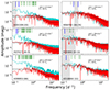 |
Fig. 3. Frequency spectra of selected BSGs. We show the periodograms calculated at the beginning (cyan) and the end (red) of the pre-whitening process. The vertical lines at the top of each panel point to the different types of identified frequencies: independent (solid), harmonics (dashed), and combinations (dotted). The solid black line corresponds to the best-fit SLF variability model (Eq. (4)) that we adopt for the star. The gray-shaded region indicates the range of frequencies that can be identified as being due to the stellar rotation. |
3.2. Stochastic low-frequency variability
Altogether, the amplitude spectra of the Galactic BSGs illustrate a background signal that is indicative of SLF variability. It has the form of a broad excess in the amplitude at low frequencies (red noise); this is followed by a decline of 1−2 orders of magnitude, reaching the level that is described as white noise. The stochastically excited signal is parameterized by a Lorentzian-like profile (Stanishev et al. 2002; Blomme et al. 2011) that is typically employed for describing its properties (e.g., Bowman et al. 2019b, 2020; Dorn-Wallenstein et al. 2020; Shen et al. 2024).
At each step of the iterative pre-whitening process, we fit the amplitude (residual) spectra with the function
 (4)
(4)
where α0 the amplitude of the red noise as v → 0, τ the characteristic timescale, γ the slope of the decay, and αw the white-noise term. The fit of the data was performed in the frequency range 0.07−25 d−1 using the optimize.curve_fit routine from the scipy package (Virtanen et al. 2020). The error estimates were assessed from the covariance matrix. We evaluated the quality of the fit using a standard χ2 calculation.
We terminated the iterative process as soon as the relative change between the χ2 values of two successive iterations fell below the tolerance value of 0.1 for five iterations in a row. The signal-to-noise ratio (S/N) values of the prior extracted frequencies were then updated in order to comply with the latest computed model. For describing the SLF variability of a star with multiple observing windows, we adopted the fit model with the lowest χ2, which we display in logarithmic scale in Fig. 3 (black curve). The base 10 logarithm of the fit values of α0 and αw, along with the values of τ and γ, are listed in Table A.2.
3.3. Metrics of the time domain
As for a statistical measure of the photometric scatter, we calculated the standard deviation of the magnitude measurements, Xi:
 (5)
(5)
where  is the mean magnitude of the light curve and N the number of data points. The alternative and less sensitive to outliers median absolute deviation was also explored; as it delivered almost identical to σ results, it is here omitted.
A robust method for assessing the independence of successive measurements is the coherency parameter, ψ2. It characterizes the level of stochasticity in the time-series data by evaluating the correlation between the sequential measurements against the white noise. It is defined on the basis of the zero-crossings Dk, namely the number of times that the signal crosses the zero level. The nonnegative integer k is the order in the time-series differences, such that
 (6)
(6)
with X0, i pointing to the original dataset Xi. For measuring Dk, the “clipped” data points Zk, i are first generated from Xk, i as
 (7)
(7)
wherefrom Dk is calculated as the sum of the squared consecutive differences and normalized to their size,
 (8)
(8)
Finally, ψ2 is calculated sufficiently from the first five orders (Kuszlewicz et al. 2020) as
 (9)
(9)
where Δk denotes the increments of the k-order crossings:
 (10)
(10)
and ϕk is the respective increments of a white-noise signal. The ϕk values were calculated from a Gaussian-distributed sample of data points that was generated over the studied grid of the TESS timestamps.
Finally, we evaluated the asymmetry of the light curves using the moment measure of skewness, which is defined as
 (11)
(11)
The metric has a positive (negative) value when the distribution of measurements is right (left) skewed, and equals to zero when it is symmetric.
The calculated values of the above statistical measures are provided in Table A.2. These were taken as the average values of measurements obtained across the different observing windows. Uncertainties are taken as the 1-sigma values.
4. Spectral energy distributions
Our aim is to investigate the association between variability features and fundamental stellar parameters. While log Teff and log g for our sample stars have been determined by Fraser et al. (2010), their analysis did not provide stellar luminosities. To retrieve these, we modeled the SED of the objects.
We constrained the blue part of the SEDs with UBV photometry from Mermilliod (2006) and with data from the Naval Observatory Merged Astrometric Dataset (NOMAD; Zacharias et al. 2004) that extend to the R band. We included recent photometry from Gaia DR3 in the G, GBP, and GRP bands, which in general was found to be in good agreement with the earlier measurements. Near-infrared photometry was taken from 2MASS (Cutri et al. 2003), whereas data from the AllWISE catalog (Cutri et al. 2014) were employed for describing the SEDs up to 22 μm. To better constrain the flux in the mid-infrared, we also included photometry from the AKARI satellite (Ishihara et al. 2010) and the Midcourse Space Experiment (MSX; Egan et al. 2003). We collected the photometric counterparts by cross-matching between the stellar coordinates and the above catalogs, using a search radius of 2″ for the optical and 2MASS studies and 5″ for the mid-infrared ones that have a lower spatial resolution. The conversion between magnitudes and fluxes was performed based on the passband zero points and effective wavelengths, which are available by the SVO Filter Profile Service3.
We fitted the multiband photometry within a standard optimization procedure using the public available grids of synthetic spectra generated with the TLUSTY code (OSTAR2002 and BSTAR2006; Lanz & Hubeny 2007). We selected model SEDs with solar abundances. As the lower limit of the BSTAR2006 grid is 15 000 K, we fit the data of our cooler seven stars with theoretical SEDs from Howarth (2011), which are generated with the ATLAS9 code.
The flux at wavelength λ (fλ) that is received from a star with radius R at distance D and reddened with extinction A(λ) is given as
 (12)
(12)
where Fλ is the flux emerging from the stellar surface and C = R/D. We ran a Levenberg-Marquardt method to minimize the residuals between Eq. (12) and the photometry, leaving free the scaling factor, C, and the visual extinction, AV (e.g., as in Kourniotis et al. 2015, 2022). Relative to AV, the extinction at λ was expressed using the law from Cardelli et al. (1989) and assuming RV = 3.1. The flux per unit surface area, Fλ ≡ Fλ(Teff, log g), was determined for each star by interpolating within the grid of synthetic models.
The photometry and best-fit models for selected stars are displayed in Fig. 4, and for the entire sample in the external appendix on Zenodo. For several cases, a weak offset between the model flux and the observations in the infrared implies excess due to stellar winds. In Table A.3 we list the base 10 logarithms of C (expressed in units of R⊙/pc) that we used to determine the stellar radii, and thus the luminosities, from the distances to the objects. In this work, the distances were taken as the photogeometric estimates from Gaia DR3 (Bailer-Jones et al. 2021) and are listed in Table A.3 along with the resulting log (L/L⊙) values.
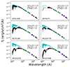 |
Fig. 4. SEDs of selected BSGs. Data were taken from Mermilliod (2006, black circles), NOMAD (blue crosses), Gaia DR3 (red asterisks), 2MASS (green triangles), WISE (green rhombi), AKARI (magenta squares), and MSX (blue diamonds). The best-fit TLUSTY model (ATLAS9 for HD 74371) is overplotted, un-reddened (cyan line) and reddened according to the inferred AV (black line). In each panel, we display the stellar designation (lower left) and parameters (upper right). |
5. Results and discussion
In the current section, we present and discuss associations between the physical and evolutionary properties of the stars and the features extracted from the analysis of variability.
With the stellar luminosities measured, we locate our studied objects in the Hertzsprung-Russell diagram of Fig. 5, and superimpose them on models of stellar evolution at solar metallicity (Ekström et al. 2012). The tracks assume an initial rotational velocity at 40% of the critical speed. As can be seen, the sample stars span evolutionary tracks beyond the end of the main-sequence phase in the range Mini = 9 − 40 M⊙. In the same plot, we indicate the reported α Cygni variables using large outer circles, which occupy the upper right region of the evolutionary diagram. The α Cygni variables are in good agreement with the definition of post-RSGs, meaning they span tracks that suggest blueward evolution (5.0 ≲ log(L/L⊙)≲5.8).
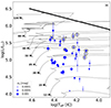 |
Fig. 5. Hertzsprung-Russell diagram for the evolution of massive stars. Theoretical tracks at solar metallicity are taken from Ekström et al. (2012) for stars rotating initially at 40% of their critical velocity. The size of the markers is proportional to the amplitude of the SLF variability (Sect. 5.3). The variables of the α Cygni class are indicated by outer circles, and the thick line represents the Humphreys-Davidson limit. The uncertainty in the spectroscopic temperature is illustrated by the error bar on the upper right. |
As for an inherently spectroscopic assessment and alternative to the SED-based luminosity, we additionally calculated the Eddington factor Γe of the studied objects (Table A.3). The parameter is a function of the so-called spectroscopic luminosity (Langer & Kudritzki 2014) and is defined as
 (13)
(13)
where σB is the Stefan-Boltzmann constant, c the speed of light, and κe = 0.4 cm2g−1 the opacity, here assuming only due to photon scattering by free electrons.
5.1. Correlations in the time domain
In Fig. 6 we present the plots of log Teff, log (L/L⊙) , and Γe against the calculated metrics of the time domain. To assess whether the relationship between two parameters is monotonic, we show at the lower right of each panel the Spearman’s rank correlation coefficient rs. Outliers were excluded from this calculation by masking values whose absolute difference from the median exceeded five times the median absolute deviation.
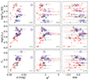 |
Fig. 6. Stellar parameters of BSGs against their time-domain statistics. Red points indicate the cROT variables, and black points the nROT ones. The outer circles indicate the α Cygni variables. We mark stars susceptible to TESS contamination with CROWDSAP+ values lower than 0.8 (“X” symbols) and within 0.8 − 0.9 (“x” symbols). We include HD 94493 in the latter category due to its proximity to a bright source located outside the photometric aperture. |
The strongest correlation found in this study is the positive trend between σ and log (L/L⊙) (rs = 0.74, p < 0.0001), which decodes into a tighter relationship with Γe (rs = 0.77, p < 0.0001). Such a correlation is already reported by the early variability studies of BSGs (Maeder & Rufener 1972; Maeder 1980), and mirrors, to a certain extent4, the corresponding trend that is reported between the luminosity and the amplitude of SLF variability (Bowman et al. 2019b, 2020). Here, the extreme outlier star (σ ∼ 0.03) is the α Cygni variable HD 77581 (Fig. 1), which, as previously mentioned, is a member of the eclipsing binary Vela X–1. This star has long been known to possess an enigmatic light curve that is modulated by effects such as gravitational distortion (Jones & Liller 1973), gas streaming (Blondin et al. 1991), and non-radial oscillations of the BSG, which are tidally induced by the companion pulsar (Quaintrell et al. 2003).
Positive correlation is also seen between ψ2 and log (L/L⊙) (rs = 0.52, p < 0.001), indicating that the more luminous (and higher amplitude) variables possess smooth light curves with a higher degree of coherency compared to less luminous ones (e.g., also Bowman & Dorn-Wallenstein 2022). Moreover, the highest ψ2 values are found to largely fluctuate across different TESS sectors. With several of these cases being flagged as cROT variables, these stars could be subject to an ephemeral modulation induced by rotation that emerges on top of their pulsational activity. On the other hand, the less luminous BSGs (log (L/L⊙) < 5) are prone to a noise-like photometric behavior, and the vast majority are identified as cROT stars. Their variability may therefore be explained by the presence of surface spots and/or corotating inhomogeneities in the wind (Morel et al. 2004; Aerts et al. 2013; Balona et al. 2015; Burssens et al. 2020), with the latter features growing with increasing mass loss (thus with increasing luminosity; Krtička et al. 2021). The positive correlation between Γe and the skewness (rs = 0.33, p = 0.04; Fig. 6) could be evidence in favor of the latter scenario; winds structured by line-driven instabilities are linked to short-term brightening of the stars, producing thus time series that are negatively skewed (Krtička & Feldmeier 2021).
Several α Cygni variables within the upper luminous sample appear to be less bound to the above trends. Moreover, other luminous stars5 (log (L/L⊙) ≳ 5.1), as well as the less luminous nROT variable HD 105071 (with ψ2 = 2.0 ± 0.5; Fig. 6), exhibit the α Cygni phenomenon in their light curves, and are marked as “candidate” α Cygni variables in the HIPPARCOS study of Lefèvre et al. (2009). Collectively, the irregularity in the photometric data of these objects follows the realization that they are not homogeneous with respect to the excitation mechanisms of their pulsations, these including oscillatory convection modes and radial strange modes (Gautschy 2009; Saio 2011; Saio et al. 2013). On top of this activity, a structured and/or variable wind has been reported in stars of the class (Chesneau et al. 2014; Kraus et al. 2015; Cidale et al. 2023).
5.2. Correlations with the independent frequencies
In Fig. 7 we display the total of the independent frequencies, fi, extracted and their amplitudes, Ai, as functions of the log Teff (upper panel) and log (L/L⊙) (lower panel). The number of the frequencies fi per observing window does not exceed three. Accordingly, the number of “individual” frequencies per star (under the Rayleigh resolution) that were extracted from the different windows is less than five. Nonetheless, no clear association is found between these metrics and the stellar parameters. We note a disposition of the hotter and less luminous BSGs toward higher frequencies. Since these BSGs have the lowest S/N values, such an observation is apparently sensitive to the extraction process followed (e.g., the termination criterion for the pre-whitening process and the noise or significance level adopted). The distribution of Ai mirrors that of σ (Fig. 6), linking the photometric dispersion of stars with log (L/L⊙) ≳ 5 to significant (quasi-)periodic cycles, whereas moving to the less luminous BSGs, variability is instead described as blends of weak low-amplitude signals.
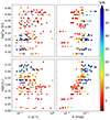 |
Fig. 7. Stellar parameters against frequencies fi and their amplitudes, Ai, which are extracted from the periodograms of all observing windows. The data are color coded with respect to their S/N. |
A more comprehensive view of the plot in Fig. 7 is shown in the histograms of Fig. 8, which show the distribution of fi as functions of log Teff (upper panel) and log (L/L⊙) (lower panel). To build the histograms, we employed the individual frequencies per star, that is, we grouped the frequencies extracted from the different windows and bin-averaged them. The size of the bin was chosen to be 0.05 d−1 and approximate to the Rayleigh resolution. Then, for each of the two stellar parameters we split the sample by the 33rd and 66th percentile, forming three nearly equal size groups. Their histograms are illustrated with different color/shape; solid blue (p0 to p33), dashed green (p33 to p66), and dotted red (p66 to p100). The interval parameter values are given in the legend. As the data display positive skewness, we fit the histograms to gamma distributions following the two-variable parameterization, with a probability density function of
 (14)
(14)
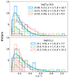 |
Fig. 8. Histograms of the individual BSG frequencies as functions of log Teff (upper panel) and log (L/L⊙) (lower panel). In each plot, the sample is split into three groups based on the parameter values (see the legend). The histograms for the α Cygni variables are indicated with cross-hatching. |
where Γ(α) is the gamma function. The calculated fit models are displayed in Fig. 8 as thick curves; their parameters are provided in the legend.
The inspection of the grouped data as a function of the stellar temperature (Fig. 8, upper panel) reveals that the hot BSGs of the sample with log Teff ≥ 4.34 display shift of their frequencies to higher values. The high-frequency tail recedes with decreasing temperature such that, in the cooler groups, frequencies become heavily centered around ∼0.13 d−1. This effect, however, is produced by the higher fraction of the contained α Cygni variables. Their identified frequencies are dispersed modestly around ∼0.13 d−1 and confined to below 0.3 d−1. Moving into the statistics on the stellar luminosity (Fig. 8, lower panel), one can tell that the aforementioned tail identifies stars of the low- and moderate-luminous groups, which share similar properties.
Summing up, the periodograms differentiate between distinct groups of stars that fall under the BSG umbrella: moderate- to high-luminosity stars showing frequencies at the lower range, the subgroup of α Cygni stars with fi < 0.3 d−1, and the younger and less massive BSGs with frequencies shifted to higher values. As the third group comprises more compact objects per se, we speculate that this effect is caused by the rotational modulation acting over shorter periods and/or the effects caused by the Coriolis force exerted on the excited modes, although the latter mechanism has been mostly observed in B-type stars in the main sequence (e.g., Salmon et al. 2014).
5.3. Correlations with the stochastic low-frequency variability
Similar to Fig. 6, Fig. 9 presents plots of the stellar parameters against the parameters of the SLF variability. To discuss the dependence of the latter on the evolutionary stage of the stars, we recalculated the Spearman’s rank correlation coefficient for each parameter set having excluded the α Cygni stars (bold font value).
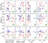 |
Fig. 9. Same as Fig. 6 but for the parameters log αw, log α0, τ, γ, of the SLF variability models. The bold font value shows the Spearman’s rank correlation coefficient for a set of parameters; the α Cygni variables are excluded. |
A significant positive correlation is seen between the red-noise amplitude and log Teff (rs = 0.59, p < 0.0001) that persists with excluded (and within) the group of α Cygni variables (rs = 0.53, p = 0.002). This information is illustrated in the Hertzsprung-Russell diagram in Fig. 5, where the marker size is proportional to α0. Our results suggest that the background signal is more pronounced at earlier stages of evolution and drops as the stars age. Interestingly, an inverse association between these two parameters has been reported by studies on early-type stars spanning the upper main sequence (Bowman et al. 2020; Shen et al. 2024). Complementing with the present findings over a more evolved sample lets us speculate that SLF variability is amplified at or shortly after the end of the main-sequence phase.
From Fig. 9, it can also be seen that the characteristic timescale τ is negatively correlated with log Teff (rs = −0.28, p = 0.08), which is in line with the reported decrease in the corresponding characteristic frequency of the signal toward more evolved stars (Shiode et al. 2013; Bowman et al. 2020; Vanon et al. 2023; Shen et al. 2024). The nonsignificant positive trend between τ and Γe (rs = 0.23) then mirrors the inverse association of τ with log g, whereas no association is seen between τ and log (L/L⊙). The slope, γ, of the red noise, on the other hand, is shown to be most related with log (L/L⊙) , though not significantly (rs = 0.18, when excluding the α Cygni stars6). Weak (or no) correlations are observed between the stellar parameters and the level of the white noise, αw.
Studies of young massive stars have highlighted the positive trend between the amplitude of SLF variability and luminosity (e.g., Bowman et al. 2020; Shen et al. 2024), which is interpreted as being due to the higher convective velocities with increasing stellar mass and core luminosity (e.g., Shiode et al. 2013; Ratnasingam et al. 2023; Anders et al. 2023). This trend is insensitive to the parameter of metallicity, which serves as evidence of the core-excited nature of the background signal, especially for stars at young stages (Bowman et al. 2019a, 2024).
At first glance, the analysis of the current, post-main-sequence, sample suggests that log α0 and the stellar (and spectroscopic) luminosities are unrelated (Fig. 9). A positive, yet nonsignificant, trend between these parameters is shown when one excludes the α Cygni variables. We compare this questionable trend to the relevant findings from Bowman et al. (2019a) in the LMC. Using TESS data, these authors extracted the parameters of the SLF variability from 53 BSGs with spectral type earlier than B4. For our purpose we calculated, and provide in Table A.3, the absolute magnitudes in G-band of our sample stars from
 (15)
(15)
using the values of distance D from Gaia (Table A.3). The G-band extinction was estimated from our SED-estimated extinction in the visual considering that AG ≃ 0.77AV (Sanders & Das 2018).
In Fig. 10 we display MG against log α0, color coding the markers as a function of log Teff. The variables of the α Cygni class (with large outer circles) appear confined below −6.4 mag (vertical thin line). Considering that possible unidentified α Cygni stars would occupy the same area on the plot (see also Sect. 5.1), we focus on the 25 BSGs that are fainter than this threshold. As expected from our above discussion, a nonsignificant weak (negative) trend is measured between the amplitude of the SLF variability with decreasing MG (rs = −0.08). We depict the linear fit to the truncated sample using a solid thick line.
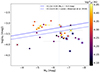 |
Fig. 10. Absolute G−band magnitudes vs. log α0. The markers are color coded as a function of log Teff. The designation for the α Cygni variables and for stars susceptible to TESS contamination follows that in Fig. 6. We show the linear fit to BSGs with MG fainter than –6.4 mag (thick solid line). The fit (+offset) to the respective parameters of BSGs in the LMC is displayed (dashed line; Bowman et al. 2019a). |
An important remark by Bowman et al. (2019a) is the absence of coherent frequencies in the LMC sample, which led the authors to model the SLF variability without pre-whitening their data. As pre-whitening wears down the amplitude spectra (see, e.g., Fig. 3), the relevant properties are expected to be systematically offset compared to when the original data are modeled instead7. Such a speculation is also evident within the study of Bowman et al. (2019a) where a sample of eclipsing stars was explored additional to their BSGs, nevertheless following pre-whitening of their signal peaks. When comparing between those two samples, the measured values for the red-noise level are shown to be systematically offset (their Fig. 4). We display the fit model from the discussed study in our Fig. 10 as a dashed thick line. For the sake of comparison, an arbitrary constant is added to it in order to match the mean level of our data8.
Similar trends are found between the study of Bowman et al. (2019a) and the current work when confining ourselves to lower luminosities (Fig. 10). In this regime, one may speculate about a metallicity-independent mechanism for driving the SLF variability, such as core convection. Furthermore, as seen in Fig. 9, the vast majority of variables with log (L/L⊙) ≲ 5 display 2 ≲ γ ≲ 4, which match, in general, the power-law exponents of the model spectra generated by core-excited IGWs (Edelmann et al. 2019). We do stress that a larger statistical sample is essential for establishing the present result, given the sparsity of our sample toward the low-luminosity end where also the TESS data of HD 141318 are susceptible to contaminating flux (CROWDSAP+ = 0.842). The results from the current study make also less plausible the scenario that SLF variability is generated by subsurface convection zones driven by the iron opacity peak. The convective flux in such zones relative to the total stellar flux is expected to increase with decreasing log Teff and increasing luminosity (Cantiello et al. 2021; Shen et al. 2024), which does not comply with the current picture for the SLF variability amplitude; instead, we observe a decline in α0 toward the upper cool Hertzsprung-Russell diagram (see Fig. 5).
From Fig. 9, it is also evident that “within” the α Cygni group, no trend is evident between log α0 and either of our luminosity assessments (accordingly, between log α0 and MG, for MG ≲ −6.4; Fig. 10). Rather, these stars are en masse predisposed to lower SLF variability amplitudes. Since in this study the stellar age appears to be more influential for the SLF variability amplitudes compared to the mass, we attribute this effect to the advanced evolutionary stage of α Cygni stars. In the scenario that the SLF variability is core-excited, the suppressed signal of α Cygni variables could mirror stars with undersized cores, for example due to efficient mixing of the core material into the stellar envelope at the earlier phases. An alternative explanation would point to radiative damping of the low-frequency modes when these propagate within a density stratified envelope, with the effect becoming more prominent with the stellar age (e.g., Vanon et al. 2023). Finally, the positive association that is seen in the early stages between the red-noise amplitude and the stellar mass (Bowman et al. 2020; Shen et al. 2024) is expected to diminish upon a steep drop in the latter, as this can happen during the RSG phase via pulsation-driven superwinds (Yoon & Cantiello 2010).
6. Conclusions
We conducted a variability study of 41 post-main-sequence BSGs in the Galaxy with parameters (log Teff and log g) determined from FEROS spectroscopy (Fraser et al. 2010) and our own SED modeling to retrieve stellar luminosities. We also explored the Eddington factor, Γe, of the stars. Our analysis was performed using data from the TESS survey across Sectors 5 − 66. We described the photometric time domain by means of three statistical measures, the standard deviation, the coherency parameter (ψ2), and the skewness, to assess the degree of scatter, stochasticity, and asymmetry of the light curves, respectively. In the frequency domain, we extracted prominent frequencies via iterative pre-whitening and modeled the background signal (which is indicative of SLF variability) that manifests ubiquitously in the residual spectra.
We report a positive correlation between log (L/L⊙) and the amplitude of the TESS light curves. Stars with log (L/L⊙) ≲ 5 display independent frequencies that comply with the rotational ones, suggesting rotational modulation as a plausible mechanism for their variability. The majority of these stars display light curves with negative skewness, which has been shown to be associated with line-driven wind instability. For log (L/L⊙) ≳ 5, our sample also comprises the reported α Cygni variables (and presumably more unidentified counterparts of the class), which possess multi-period variability with diverse, in some cases time-variant, properties. The irregular light curves of these stars mirror the documented and diverse mechanisms at play, such as mixed-mode oscillations that include radial strange modes, winds, and (at least for HD 77581) binarity.
A significant positive correlation is found between log Teff and the amplitude of the SLF variability, indicating that the ambiguous signal is more pronounced at earlier phases and drops as the stars evolve beyond the main sequence. Essentially, this result contradicts the scenario that SLF variability is excited by subsurface convection. Consistent with previous findings, a negative (respectively, positive) association is seen between the characteristic timescale of the signal and log Teff (respectively, Γe).
The amplitude of the SLF variability scales weakly with the absolute G−band magnitude for stars fainter than MG ∼ −6.4 mag, the limit that here confines the α Cygni variables. Although not significant, this trend is similar to that for BSGs in the LMC (Bowman et al. 2019a), which supports the scenario that the background signal is driven by core-excited IGWs. On the other hand, this trend vanishes for the α Cygni variables, which are predisposed as a group to lower SLF variability amplitudes. Given that the stellar age appears in this work to be the most potent parameter in regulating the excitation of the signal, we suggest that the suppressed SLF variability of the α Cygni variables could mirror their rather advanced phase as post-RSG stars.
A study with a larger statistical sample would enable a more improved mapping of variability in BSGs onto the evolutionary diagram. Moreover, theoretical insights into the internal or surface processes of α Cygni stars are needed to interpret their distinctive red noise. It is yet to be determined whether these stars undergo changes in the deep interior that facilitate their mass loss at the RSG phase, and which could further justify their poorly explained surface abundances.
Data availability
An external appendix containing supplementary figures is available on the Zenodo repository at https://doi.org/10.5281/zenodo.15106993.
We here account for those stars with a solid classification, disregarding those flagged as candidates.
Particularly for stars that do not display significant isolated frequencies.
HD 92964, HD 108002, HD 109867 (ψ2 = 2.2 ± 0.4), HD 111973, HD 115842, HD 152235, and HD 154090.
The outlier nROT star with γ ∼ 6 is HD 105071, which as earlier mentioned is a candidate α Cygni variable. Given also its large ψ2 value, we suggest that the distance to the target may be underestimated.
For testing purposes, we explored our sample using the original amplitude spectra and confirm the effect.
This constant accounts also for the conversion among units.
Acknowledgments
We thank the anonymous referee for providing a detailed report that greatly improved the quality of this work. The project has received funding from the European Union’s Framework Programme for Research and Innovation Horizon 2020 (2014–2020) under the Marie Skłodowska-Curie grant agreement no. 823734. LC acknowledges financial support from CONICET (PIP 1337) and the University of La Plata (Programa de Incentivos 11/G160). The Astronomical Institute Ondřejov is supported by RVO:67985815. MRD acknowledges support from a CONICET fellowship. This research has made use of the SIMBAD data base, operated at CDS, Strasbourg, France.
References
- Aerts, C., Puls, J., Godart, M., & Dupret, M. A. 2009, A&A, 508, 409 [NASA ADS] [CrossRef] [EDP Sciences] [Google Scholar]
- Aerts, C., Lefever, K., Baglin, A., et al. 2010, A&A, 513, L11 [NASA ADS] [CrossRef] [EDP Sciences] [Google Scholar]
- Aerts, C., Simón-Díaz, S., Catala, C., et al. 2013, A&A, 557, A114 [NASA ADS] [CrossRef] [EDP Sciences] [Google Scholar]
- Aerts, C., Símon-Díaz, S., Bloemen, S., et al. 2017, A&A, 602, A32 [NASA ADS] [CrossRef] [EDP Sciences] [Google Scholar]
- Aerts, C., Bowman, D. M., Símon-Díaz, S., et al. 2018, MNRAS, 476, 1234 [NASA ADS] [CrossRef] [Google Scholar]
- Aerts, C., Mathis, S., & Rogers, T. M. 2019, ARA&A, 57, 35 [Google Scholar]
- Anders, E. H., Lecoanet, D., Cantiello, M., et al. 2023, Nat. Astron., 7, 1228 [NASA ADS] [CrossRef] [Google Scholar]
- Bailer-Jones, C. A. L., Rybizki, J., Fouesneau, M., Demleitner, M., & Andrae, R. 2021, AJ, 161, 147 [Google Scholar]
- Balona, L. A., Baran, A. S., Daszyńska-Daszkiewicz, J., & De Cat, P. 2015, MNRAS, 451, 1445 [Google Scholar]
- Bellinger, E. P., de Mink, S. E., van Rossem, W. E., & Justham, S. 2024, ApJ, 967, L39 [NASA ADS] [CrossRef] [Google Scholar]
- Blomme, R., Mahy, L., Catala, C., et al. 2011, A&A, 533, A4 [NASA ADS] [CrossRef] [EDP Sciences] [Google Scholar]
- Blondin, J. M., Stevens, I. R., & Kallman, T. R. 1991, ApJ, 371, 684 [NASA ADS] [CrossRef] [Google Scholar]
- Bowman, D. M. 2020, Front. Astron. Space Sci., 7, 70 [Google Scholar]
- Bowman, D. M., & Dorn-Wallenstein, T. Z. 2022, A&A, 668, A134 [NASA ADS] [CrossRef] [EDP Sciences] [Google Scholar]
- Bowman, D. M., Burssens, S., Pedersen, M. G., et al. 2019a, Nat. Astron., 3, 760 [Google Scholar]
- Bowman, D. M., Aerts, C., Johnston, C., et al. 2019b, A&A, 621, A135 [NASA ADS] [CrossRef] [EDP Sciences] [Google Scholar]
- Bowman, D. M., Burssens, S., Simón-Díaz, S., et al. 2020, A&A, 640, A36 [NASA ADS] [CrossRef] [EDP Sciences] [Google Scholar]
- Bowman, D. M., Van Daele, P., Michielsen, M., & Van Reeth, T. 2024, A&A, 692, A49 [NASA ADS] [CrossRef] [EDP Sciences] [Google Scholar]
- Brasseur, C. E., Phillip, C., Fleming, S. W., Mullally, S. E., & White, R. L. 2019, Astrophysics Source Code Library [record ascl:1905.007] [Google Scholar]
- Bresolin, F., Pietrzyński, G., Urbaneja, M. A., et al. 2006, ApJ, 648, 1007 [NASA ADS] [CrossRef] [Google Scholar]
- Brott, I., de Mink, S. E., Cantiello, M., et al. 2011, A&A, 530, A115 [NASA ADS] [CrossRef] [EDP Sciences] [Google Scholar]
- Burssens, S., Simón-Díaz, S., Bowman, D. M., et al. 2020, A&A, 639, A81 [NASA ADS] [CrossRef] [EDP Sciences] [Google Scholar]
- Burssens, S., Bowman, D. M., Michielsen, M., et al. 2023, Nat. Astron., 7, 913 [NASA ADS] [CrossRef] [Google Scholar]
- Cantiello, M., Langer, N., Brott, I., et al. 2009, A&A, 499, 279 [NASA ADS] [CrossRef] [EDP Sciences] [Google Scholar]
- Cantiello, M., Lecoanet, D., Jermyn, A. S., & Grassitelli, L. 2021, ApJ, 915, 112 [NASA ADS] [CrossRef] [Google Scholar]
- Cardelli, J. A., Clayton, G. C., & Mathis, J. S. 1989, ApJ, 345, 245 [Google Scholar]
- Castro, N., Fossati, L., Langer, N., et al. 2014, A&A, 570, L13 [NASA ADS] [CrossRef] [EDP Sciences] [Google Scholar]
- Chesneau, O., Kaufer, A., Stahl, O., et al. 2014, A&A, 566, A125 [NASA ADS] [CrossRef] [EDP Sciences] [Google Scholar]
- Cidale, L. S., Haucke, M., Arias, M. L., et al. 2023, A&A, 677, A176 [NASA ADS] [CrossRef] [EDP Sciences] [Google Scholar]
- Cutri, R. M., Skrutskie, M. F., van Dyk, S., et al. 2003, VizieR Online Data Catalog: II/246 [Google Scholar]
- Cutri, R. M., Wright, E. L., Conrow, T., et al. 2014, VizieR Online Data Catalog: II/328 [Google Scholar]
- de Burgos, A., Simón-Díaz, S., Urbaneja, M. A., & Negueruela, I. 2023, A&A, 674, A212 [NASA ADS] [CrossRef] [EDP Sciences] [Google Scholar]
- Degroote, P., Aerts, C., Baglin, A., et al. 2010, Nature, 464, 259 [Google Scholar]
- Degroote, P., Aerts, C., Michel, E., et al. 2012, A&A, 542, A88 [NASA ADS] [CrossRef] [EDP Sciences] [Google Scholar]
- de Mink, S. E., Langer, N., Izzard, R. G., Sana, H., & de Koter, A. 2013, ApJ, 764, 166 [Google Scholar]
- Dorn-Wallenstein, T. Z., Levesque, E. M., & Davenport, J. R. A. 2019, ApJ, 878, 155 [NASA ADS] [CrossRef] [Google Scholar]
- Dorn-Wallenstein, T. Z., Levesque, E. M., Neugent, K. F., et al. 2020, ApJ, 902, 24 [NASA ADS] [CrossRef] [Google Scholar]
- Dorn-Wallenstein, T. Z., Levesque, E. M., Davenport, J. R. A., et al. 2022, ApJ, 940, 27 [Google Scholar]
- Edelmann, P. V. F., Ratnasingam, R. P., Pedersen, M. G., et al. 2019, ApJ, 876, 4 [NASA ADS] [CrossRef] [Google Scholar]
- Egan, M. P., Price, S. D., Kraemer, K. E., et al. 2003, VizieR Online Data Catalog: V/114 [Google Scholar]
- Ekström, S., Georgy, C., Eggenberger, P., et al. 2012, A&A, 537, A146 [Google Scholar]
- Farrell, E. J., Groh, J. H., Meynet, G., et al. 2019, A&A, 621, A22 [NASA ADS] [CrossRef] [EDP Sciences] [Google Scholar]
- Fraser, M., Dufton, P. L., Hunter, I., & Ryans, R. S. I. 2010, MNRAS, 404, 1306 [NASA ADS] [Google Scholar]
- Gaia Collaboration 2022, VizieR Online Data Catalog: I/355 [Google Scholar]
- Gautschy, A. 2009, A&A, 498, 273 [NASA ADS] [CrossRef] [EDP Sciences] [Google Scholar]
- Gebruers, S., Tkachenko, A., Bowman, D. M., et al. 2022, A&A, 665, A36 [NASA ADS] [CrossRef] [EDP Sciences] [Google Scholar]
- Georgy, C., Saio, H., & Meynet, G. 2014, MNRAS, 439, L6 [Google Scholar]
- Glatzel, W., & Kraus, M. 2024, MNRAS, 529, 4947 [Google Scholar]
- Guerrero, N. M., Seager, S., Huang, C. X., et al. 2021, ApJS, 254, 39 [NASA ADS] [CrossRef] [Google Scholar]
- Haucke, M., Cidale, L. S., Venero, R. O. J., et al. 2018, A&A, 614, A91 [NASA ADS] [CrossRef] [EDP Sciences] [Google Scholar]
- Henneco, J., Schneider, F. R. N., & Laplace, E. 2024, A&A, 682, A169 [NASA ADS] [CrossRef] [EDP Sciences] [Google Scholar]
- Howarth, I. D. 2011, MNRAS, 413, 1515 [NASA ADS] [CrossRef] [Google Scholar]
- Hubeny, I., & Lanz, T. 1995, ApJ, 439, 875 [Google Scholar]
- Ishihara, D., Onaka, T., Kataza, H., et al. 2010, A&A, 514, A1 [NASA ADS] [CrossRef] [EDP Sciences] [Google Scholar]
- Jermyn, A. S., Anders, E. H., & Cantiello, M. 2022, ApJ, 926, 221 [NASA ADS] [CrossRef] [Google Scholar]
- Jones, C., & Liller, W. 1973, ApJ, 184, L121 [Google Scholar]
- Kaufer, A., Stahl, O., Wolf, B., et al. 1997, A&A, 320, 273 [NASA ADS] [Google Scholar]
- Kaufer, A., Stahl, O., Tubbesing, S., et al. 1999, The Messenger, 95, 8 [Google Scholar]
- Kaufer, A., Stahl, O., Prinja, R. K., & Witherick, D. 2006, A&A, 447, 325 [NASA ADS] [CrossRef] [EDP Sciences] [Google Scholar]
- Klencki, J., Istrate, A., Nelemans, G., & Pols, O. 2022, A&A, 662, A56 [NASA ADS] [CrossRef] [EDP Sciences] [Google Scholar]
- Kourniotis, M., Bonanos, A. Z., Williams, S. J., et al. 2015, A&A, 582, A42 [NASA ADS] [CrossRef] [EDP Sciences] [Google Scholar]
- Kourniotis, M., Kraus, M., Maryeva, O., Borges Fernandes, M., & Maravelias, G. 2022, MNRAS, 511, 4360 [NASA ADS] [CrossRef] [Google Scholar]
- Kraus, M., Haucke, M., Cidale, L. S., et al. 2015, A&A, 581, A75 [NASA ADS] [CrossRef] [EDP Sciences] [Google Scholar]
- Kraus, M., Kourniotis, M., Arias, M. L., Torres, A. F., & Nickeler, D. H. 2023, Galaxies, 11, 76 [NASA ADS] [CrossRef] [Google Scholar]
- Krtička, J., & Feldmeier, A. 2021, A&A, 648, A79 [NASA ADS] [CrossRef] [EDP Sciences] [Google Scholar]
- Krtička, J., Kubát, J., & Krtičková, I. 2021, A&A, 647, A28 [NASA ADS] [CrossRef] [EDP Sciences] [Google Scholar]
- Kudritzki, R.-P., Urbaneja, M. A., Gazak, Z., et al. 2012, ApJ, 747, 15 [CrossRef] [Google Scholar]
- Kuszlewicz, J. S., Hekker, S., & Bell, K. J. 2020, MNRAS, 497, 4843 [NASA ADS] [CrossRef] [Google Scholar]
- Labadie-Bartz, J., Carciofi, A. C., Henrique de Amorim, T., et al. 2022, AJ, 163, 226 [NASA ADS] [CrossRef] [Google Scholar]
- Langer, N., & Kudritzki, R. P. 2014, A&A, 564, A52 [NASA ADS] [CrossRef] [EDP Sciences] [Google Scholar]
- Lanz, T., & Hubeny, I. 2007, ApJS, 169, 83 [CrossRef] [Google Scholar]
- Lecoanet, D., Cantiello, M., Quataert, E., et al. 2019, ApJ, 886, L15 [Google Scholar]
- Lefever, K., Puls, J., & Aerts, C. 2007, A&A, 463, 1093 [NASA ADS] [CrossRef] [EDP Sciences] [Google Scholar]
- Lefèvre, L., Marchenko, S. V., Moffat, A. F. J., & Acker, A. 2009, A&A, 507, 1141 [NASA ADS] [CrossRef] [EDP Sciences] [Google Scholar]
- Lightkurve Collaboration (Cardoso, J. V. d. M., et al.) 2018, Astrophysics Source Code Library [record ascl:1812.013] [Google Scholar]
- Ma, L., Johnston, C., Bellinger, E. P., & de Mink, S. E. 2024, ApJ, 966, 196 [NASA ADS] [CrossRef] [Google Scholar]
- Maeder, A. 1980, A&A, 90, 311 [NASA ADS] [Google Scholar]
- Maeder, A., & Rufener, F. 1972, A&A, 20, 437 [NASA ADS] [Google Scholar]
- Martinet, S., Meynet, G., Ekström, S., et al. 2021, A&A, 648, A126 [NASA ADS] [CrossRef] [EDP Sciences] [Google Scholar]
- Menon, A., Ercolino, A., Urbaneja, M. A., et al. 2024, ApJ, 963, L42 [NASA ADS] [CrossRef] [Google Scholar]
- Mermilliod, J. C. 2006, VizieR Online Data Catalog: II/168 [Google Scholar]
- Meynet, G., Chomienne, V., Ekström, S., et al. 2015, A&A, 575, A60 [NASA ADS] [CrossRef] [EDP Sciences] [Google Scholar]
- Morel, T., Marchenko, S. V., Pati, A. K., et al. 2004, MNRAS, 351, 552 [NASA ADS] [CrossRef] [Google Scholar]
- Nazé, Y., Rauw, G., & Gosset, E. 2021, MNRAS, 502, 5038 [CrossRef] [Google Scholar]
- Oudmaijer, R. D., Davies, B., de Wit, W. J., & Patel, M. 2009, in Astronomical Society of the Pacific Conference Series, eds. D. G. Luttermoser, B. J. Smith, & R. E. Stencel, 412, 17 [Google Scholar]
- Paegert, M., Stassun, K. G., Collins, K. A., et al. 2021, ArXiv e-prints [arXiv:2108.04778] [Google Scholar]
- Pedersen, M. G., Chowdhury, S., Johnston, C., et al. 2019, ApJ, 872, L9 [Google Scholar]
- Quaintrell, H., Norton, A. J., Ash, T. D. C., et al. 2003, A&A, 401, 313 [NASA ADS] [CrossRef] [EDP Sciences] [Google Scholar]
- Ratnasingam, R. P., Rogers, T. M., Chowdhury, S., et al. 2023, A&A, 674, A134 [NASA ADS] [CrossRef] [EDP Sciences] [Google Scholar]
- Ricker, G. R., Winn, J. N., Vanderspek, R., et al. 2015, J. Astron. Telescopes Instrum. Syst., 1, 014003 [Google Scholar]
- Rogers, T. M., Lin, D. N. C., McElwaine, J. N., & Lau, H. H. B. 2013, ApJ, 772, 21 [NASA ADS] [CrossRef] [Google Scholar]
- Saio, H. 2011, MNRAS, 412, 1814 [Google Scholar]
- Saio, H., Kuschnig, R., Gautschy, A., et al. 2006, ApJ, 650, 1111 [NASA ADS] [CrossRef] [Google Scholar]
- Saio, H., Georgy, C., & Meynet, G. 2013, MNRAS, 433, 1246 [NASA ADS] [CrossRef] [Google Scholar]
- Salmon, S. J. A. J., Montalbán, J., Reese, D. R., Dupret, M. A., & Eggenberger, P. 2014, A&A, 569, A18 [NASA ADS] [CrossRef] [EDP Sciences] [Google Scholar]
- Samus, N. N., Kazarovets, E. V., Durlevich, O. V., Kireeva, N. N., & Pastukhova, E. N. 2017, Astron. Rep., 61, 80 [Google Scholar]
- Sanders, J. L., & Das, P. 2018, MNRAS, 481, 4093 [CrossRef] [Google Scholar]
- Schultz, W. C., Bildsten, L., & Jiang, Y.-F. 2022, ApJ, 924, L11 [NASA ADS] [CrossRef] [Google Scholar]
- Shen, D.-X., Zhu, C.-H., Lü, G.-L., Lu, X.-Z., & He, X.-L. 2024, ApJS, 275, 2 [Google Scholar]
- Shiode, J. H., Quataert, E., Cantiello, M., & Bildsten, L. 2013, MNRAS, 430, 1736 [NASA ADS] [CrossRef] [Google Scholar]
- Simón-Díaz, S., Herrero, A., Uytterhoeven, K., et al. 2010, ApJ, 720, L174 [CrossRef] [Google Scholar]
- Simón-Díaz, S., Aerts, C., Urbaneja, M. A., et al. 2018, A&A, 612, A40 [NASA ADS] [CrossRef] [EDP Sciences] [Google Scholar]
- Southworth, J., Bowman, D. M., Tkachenko, A., & Pavlovski, K. 2020, MNRAS, 497, L19 [Google Scholar]
- Spejcher, B., Richardson, N. D., Pablo, H., et al. 2025, AJ, 169, 128 [Google Scholar]
- Stanishev, V., Kraicheva, Z., Boffin, H. M. J., & Genkov, V. 2002, A&A, 394, 625 [NASA ADS] [CrossRef] [EDP Sciences] [Google Scholar]
- Thompson, W., Herwig, F., Woodward, P. R., et al. 2024, MNRAS, 531, 1316 [NASA ADS] [CrossRef] [Google Scholar]
- Urbaneja, M. A., Kudritzki, R.-P., Bresolin, F., et al. 2008, ApJ, 684, 118 [NASA ADS] [CrossRef] [Google Scholar]
- Vanderspek, R., Doty, J., Fausnaugh, M., et al. 2018, TESS Instrument Handbook, Tech. Rep., Kavli Institute for Astrophysics and Space Science, Massachusetts Institute of Technology [Google Scholar]
- Vanon, R., Edelmann, P. V. F., Ratnasingam, R. P., Varghese, A., & Rogers, T. M. 2023, ApJ, 954, 171 [Google Scholar]
- Virtanen, P., Gommers, R., Oliphant, T. E., et al. 2020, Nat. Methods, 17, 261 [Google Scholar]
- Yoon, S.-C., & Cantiello, M. 2010, ApJ, 717, L62 [NASA ADS] [CrossRef] [Google Scholar]
- Zacharias, N., Monet, D. G., Levine, S. E., et al. 2004, Am. Astron. Soc. Meeting Abstr., 205, 48.15 [Google Scholar]
Appendix A: Supplementary tables
Studied BSGs in the Galaxy.
Statistical measures of the TESS light curves and parameters of the SLF variability.
Eddington factors (Γe) and SED-fit parameters for the sample BSGs.
Appendix B: Independent frequencies
Independent frequencies of the studied BSGs that were extracted via the iterative pre-whitening process. The resolution of the process over the different windows (consisting of single or stitched consecutive sectors) is determined by the Rayleigh criterion. The S/N values are calculated with respect to the adopted model of the SLF variability.
Frequencies and their parameters.
All Tables
Statistical measures of the TESS light curves and parameters of the SLF variability.
All Figures
|
Fig. 1. Time-series photometry from TESS of selected BSGs. Data are detrended, normalized, and converted into units of magnitude. For each star, we show data from different sectors over multiple panels. Consecutive sectors are joined together, and their numbers are displayed at the bottom of each panel. |
| In the text | |
|
Fig. 2. Iterative pre-whitening for the extraction of frequencies for HD 94493 (Sectors 63 and 64). Left: Calculated amplitude spectra (Lomb-Scargle periodograms) shown in logarithmic scale. A vertical line at the top of each panel points toward the extracted frequency, which is reported in the lower left. Right: Light curve of the star (black points) with the integrated fit model of sinusoidals superimposed (red). |
| In the text | |
|
Fig. 3. Frequency spectra of selected BSGs. We show the periodograms calculated at the beginning (cyan) and the end (red) of the pre-whitening process. The vertical lines at the top of each panel point to the different types of identified frequencies: independent (solid), harmonics (dashed), and combinations (dotted). The solid black line corresponds to the best-fit SLF variability model (Eq. (4)) that we adopt for the star. The gray-shaded region indicates the range of frequencies that can be identified as being due to the stellar rotation. |
| In the text | |
|
Fig. 4. SEDs of selected BSGs. Data were taken from Mermilliod (2006, black circles), NOMAD (blue crosses), Gaia DR3 (red asterisks), 2MASS (green triangles), WISE (green rhombi), AKARI (magenta squares), and MSX (blue diamonds). The best-fit TLUSTY model (ATLAS9 for HD 74371) is overplotted, un-reddened (cyan line) and reddened according to the inferred AV (black line). In each panel, we display the stellar designation (lower left) and parameters (upper right). |
| In the text | |
|
Fig. 5. Hertzsprung-Russell diagram for the evolution of massive stars. Theoretical tracks at solar metallicity are taken from Ekström et al. (2012) for stars rotating initially at 40% of their critical velocity. The size of the markers is proportional to the amplitude of the SLF variability (Sect. 5.3). The variables of the α Cygni class are indicated by outer circles, and the thick line represents the Humphreys-Davidson limit. The uncertainty in the spectroscopic temperature is illustrated by the error bar on the upper right. |
| In the text | |
|
Fig. 6. Stellar parameters of BSGs against their time-domain statistics. Red points indicate the cROT variables, and black points the nROT ones. The outer circles indicate the α Cygni variables. We mark stars susceptible to TESS contamination with CROWDSAP+ values lower than 0.8 (“X” symbols) and within 0.8 − 0.9 (“x” symbols). We include HD 94493 in the latter category due to its proximity to a bright source located outside the photometric aperture. |
| In the text | |
|
Fig. 7. Stellar parameters against frequencies fi and their amplitudes, Ai, which are extracted from the periodograms of all observing windows. The data are color coded with respect to their S/N. |
| In the text | |
|
Fig. 8. Histograms of the individual BSG frequencies as functions of log Teff (upper panel) and log (L/L⊙) (lower panel). In each plot, the sample is split into three groups based on the parameter values (see the legend). The histograms for the α Cygni variables are indicated with cross-hatching. |
| In the text | |
|
Fig. 9. Same as Fig. 6 but for the parameters log αw, log α0, τ, γ, of the SLF variability models. The bold font value shows the Spearman’s rank correlation coefficient for a set of parameters; the α Cygni variables are excluded. |
| In the text | |
|
Fig. 10. Absolute G−band magnitudes vs. log α0. The markers are color coded as a function of log Teff. The designation for the α Cygni variables and for stars susceptible to TESS contamination follows that in Fig. 6. We show the linear fit to BSGs with MG fainter than –6.4 mag (thick solid line). The fit (+offset) to the respective parameters of BSGs in the LMC is displayed (dashed line; Bowman et al. 2019a). |
| In the text | |
Current usage metrics show cumulative count of Article Views (full-text article views including HTML views, PDF and ePub downloads, according to the available data) and Abstracts Views on Vision4Press platform.
Data correspond to usage on the plateform after 2015. The current usage metrics is available 48-96 hours after online publication and is updated daily on week days.
Initial download of the metrics may take a while.