| Issue |
A&A
Volume 697, May 2025
|
|
|---|---|---|
| Article Number | A23 | |
| Number of page(s) | 19 | |
| Section | Extragalactic astronomy | |
| DOI | https://doi.org/10.1051/0004-6361/202452067 | |
| Published online | 30 April 2025 | |
Dark and bright sides of the Broad Line Region clouds as seen in the FeII emission of SDSS RM 102
1
Center for Theoretical Physics, Polish Academy of Sciences, Al. Lotników 32/46, 02-668 Warsaw, Poland
2
National Institute for Astrophysics (INAF), Astronomical Observatory of Padova, IT-35122 Padova, Italy
3
Department of Physics University of Crete, Voutes University Campus, 70013 Heraklion, Greece
4
Institute of Astrophysics, Foundation for Research and Technology Hellas, N.Plastira 100, Vassilika Vouton, 70013 Heraklion, Greece
5
Key Laboratory for Particle Astrophysics, Institute of High Energy Physics, Chinese Academy of Sciences, 19B Yuquan Road, Beijing 100049, PR China
6
Astronomy Department, Universidad de Concepción, Barrio Universitario S/N, Concepción 4030000, Chile
7
Millennium Institute of Astrophysics MAS, Nuncio Monseñor Sotero Sanz 100, Of. 104, Providencia, Santiago, Chile
8
Millennium Nucleus on Transversal Research and Technology to Explore Supermassive Black Holes (TITANS), Chile
9
International Gemini Observatory/NSF NOIRLab, Casilla 603, La Serena, Chile
10
Laboratório Nacional de Astrofísica, MCTI, R. dos Estados Unidos 154, Nações, CEP 37504-364, Itajubá, Brazil
11
Department of Physics, Institute of Science, Banaras Hindu University, Varanasi - 221005, India
⋆ Corresponding author: This email address is being protected from spambots. You need JavaScript enabled to view it.
Received:
30
August
2024
Accepted:
15
March
2025
Abstract
Context. Contamination from singly ionized iron emission is one of the greatest obstacles to determining the intensity of emission lines in the UV and optical wavelength ranges.
Aims. This study presents a comprehensive analysis of the Fe II emission in the bright quasar RM 102, based on the most recent version of the CLOUDY software, with the goal of understanding the nature and the origin of the emission.
Methods. We employ a constant pressure model for the emitting clouds, instead of the customary constant density assumption. The allowed parameter range is broad, with metallicity up to 50 times the solar value and turbulent velocity up to 100 km s−1 for a subset of models. We also consider geometrical effects that could enhance the visibility of the non-illuminated faces of the clouds, as well as the presence of additional mechanical heating.
Results. Our investigation reveals that the broad line region of RM 102 is characterized by highly metallic gas. The observed Fe II features provide strong evidence for an inflow pattern geometry that favours the dark sides of clouds over isotropic emission if the heating is predominantly radiative. Solutions with mechanical heating are also an interesting option, but they require further self-consistent analysis.
Conclusions. This study underscores the critical role of the dark versus bright side interpretation for reproducing the strong Fe II features in RM 102, highlighting both the geometry of the emitting region and the presence of chemically enriched gas as fundamental factors. Additionally, we report that CLOUDY currently still lacks certain transitions in its atomic databases, which prevents it from fully reproducing some observed Fe II features in quasar spectra.
Key words: galaxies: active / quasars: emission lines / quasars: general / quasars: supermassive black holes / galaxies: Seyfert
PIFI visiting scientist.
Gemini Science Fellow.
© The Authors 2025
 Open Access article, published by EDP Sciences, under the terms of the Creative Commons Attribution License (https://creativecommons.org/licenses/by/4.0), which permits unrestricted use, distribution, and reproduction in any medium, provided the original work is properly cited.
This article is published in open access under the Subscribe to Open model. This email address is being protected from spambots. You need JavaScript enabled to view it. to support open access publication.
1. Introduction
Singly ionized iron emission (Fe II) is one of the most ubiquitous signatures in the spectra of active galactic nuclei (AGN), with emission lines spanning from the ultraviolet (UV) to the near-infrared (NIR) wavelength ranges. Especially in the UV and optical ranges, the number of transitions associated with Fe II is so high that they blend forming a pseudo-continuum. The presence of this pseudo-continuum significantly complicates the fitting of lines emitted from the Broad Line Region (BLR), creating a long-standing challenge (Sargent 1968; Collin-Souffrin et al. 1979; Joly et al. 2008).
In the optical wavelength range, the intensity of Fe II emission is connected to the critical RFeII parameter of the quasar main sequence (MS) (Boroson & Green 1992; Sulentic et al. 2000), which is defined as the ratio between Fe II emission measured in the 4434–4684 Å range and Hβ emission. In the context of the MS, the sources that emit the largest amount of radiation per unit of mass are categorized as extreme-accreting sources, or extreme population A (xA) objects. These sources are characterized by RFeII>1 and a moderate-to-high Eddington ratio (L/LEdd), typically greater than 0.1 (Panda et al. 2019a), making them the strongest Fe II emitters.
The spatial extent of the Fe II emitting region remains a matter of debate. Some studies suggest that this emission originates in a region similar to that of Hβ (Shapovalova et al. 2012; Hu et al. 2015), while others propose that the Fe II emitting region may be more extended, potentially up to twice as large (Barth et al. 2013; Panda et al. 2018; Hu et al. 2020; He et al. 2021; Lu et al. 2021). However, the assumption of single-zone emission from the BLR seems appropriate, particularly for xA sources (Marziani et al. 2001; Panda et al. 2019b; Panda 2021).
Historically, two main methods have been employed to measure Fe II emission: (1) observational templates, created by isolating Fe II emission from the rest of the known lines in the spectrum of a quasar (e.g. I Zw 1 for Vestergaard & Wilkes 2001; Marziani et al. 2009); and (2) theoretical templates, which are based on calculating the transition rates of each emission line (Bruhweiler & Verner 2008; Panda et al. 2019b).
The challenge with observational templates is that they are limited by the signal-to-noise ratio (S/N) and the wavelength coverage of the spectra. Additionally, no existing template simultaneously covers both UV and optical bands (Pandey et al. 2024; Zhang et al. 2024). Theoretical templates, on the other hand, often suffer from inconsistencies between the measured emissions in the UV and optical ranges, frequently achieving a good fit in one range but showing strong mismatches in the other (Pandey et al. 2024).
In this work, we aim to analyse the Fe II emission of the bright quasar SDSS J141352.99+523444.2 (hereafter RM 102) from the UV to the optical bands. We utilize the latest version of the radiative transfer code CLOUDY C23.01 (Chatzikos et al. 2023), incorporating the most recent atomic data, to produce photoionization simulations and investigate the nature and origin of Fe II emission. RM 102, selected from the SDSS Reverberation Mapping (SDSS-RM) catalogue (Shen et al. 2019; Pandey et al. 2024), is an ideal candidate for this study because its high S/N spectrum spans a broad wavelength range (2000–5500 Å), allowing for a comprehensive analysis of both the rest-frame UV and optical ranges.
Furthermore, reliable estimates of the Hβ and Mg II time delays are available for this object, with  days and
  days (Shen et al. 2023), with Fe II time delays expected to be consistent with those of Mg II and Hβ (Zajaček et al. 2024). Moreover, its spectrum strongly resembles the quasar composite spectrum from Vanden Berk et al. (2001), indicating that it is highly representative of the quasar population.
In this study, we consider local processes which can affect the local Fe II emissivity, such as radiative and mechanical heating, geometry (illuminated and dark sides of the clouds), microturbulence and metallicity, to better understand the physical conditions in typical quasars. We adopt a constant-pressure approach which should be more appropriate for clouds in hydrostatic equilibrium conditions. We aim to test whether this setup allows us to reproduce the observed Fe II features in RM 102, and identify the most plausible models representing the physical and geometrical conditions of the BLR.
We systematically analyse the Fe II emission of RM 102, beginning with a description of its SDSS spectrum in Section 2. Section 3 details the methodology and techniques used to disentangle the properties of our source. The results of our analysis are presented in Sect. 4. In Sect. 5, we discuss the main findings of our work. Finally, Section 6, summarizes our conclusions and suggests directions for future research. The values of the cosmological parameters adopted in this work are as follows: H0 = 70 km s−1 Mpc−1, ΩM = 0.3, and ΩΛ = 0.7.
2. Observed spectrum of RM 102
RM 102 was selected for this study due to its representative quasar characteristics, high-quality spectral data, and well-documented properties from reverberation mapping studies (Shen et al. 2019). The spectrum used in this study is a compilation of 70 spectra from the SDSS Science Archive Server (SAS), the DR161. The source did not exhibit significant variability in spectral shape, justifying the use of a compiled median spectrum to achieve a high S/N. The resulting spectrum is shown in Figure 1, with the SDSS composite spectrum from Vanden Berk et al. (2001) overlaid for comparison. The two spectra show a remarkable similarity in both the overall continuum shape and line properties, although RM 102 exhibits stronger Fe II emission than the average quasar in the Vanden Berk et al. (2001) composite spectrum. This suggests that RM 102 is highly representative of bright quasars, particularly those in the xA category.
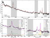 |
Fig. 1. Top: Observed spectrum of RM 102, superimposed with the SDSS composite spectrum from Vanden Berk et al. (2001). The grey shaded regions define the spectral ranges from which the Fe II emission is extracted for the red-to-blue wings ratios in the UV and optical ranges (See Sect. 3.3). The SDSS composite is normalized at λ2800 Å. Bottom left: Zoomed-in on the UV Fe II emission, outlining the different spectral components adopted during fitting. Different Fe II templates (See Table 2 for reference) are displayed in different colours. Bottom right: Zoomed-in on the optical Fe II emission, outlining the different spectral components adopted during fitting, with the various Fe II templates (See Table 2 for reference) highlighted in different colours. |
The global properties of RM 102 are summarized in Table 1, which lists its redshift (z), bolometric luminosity (Lbol), black hole mass (MBH), Eddington ratio, RFeII parameter, the measured time delay to Hβ (τHβ) and the estimated ionizing flux Φ(H) from the central engine. Φ(H) was calculated as follows: the assumed spectral energy distribution (SED) shape (Mathews & Ferland 1987) was fitted to the observed continuum in the optical band. The incident radiation was then renormalized using the redshift (i.e. the distance to the source), and the BLR distance, determined from the Hβ time delay. The ionizing photon flux above 1 Rydberg was integrated, yielding the ionizing flux Φ(H).
Basic properties of the RM 102.
The Eddington ratio of RM 102 is slightly higher than the average value of 0.17 in the SDSS quasars (Panda et al. 2018). Moreover, the RFeII = 1.24 classifies RM 102 as a ‘bona fide’ xA source, as its RFeII exceeds the lower limit of 1.0 associated with extreme Population A sources in the context of the MS (Sulentic et al. 2000; Du et al. 2016; Marziani et al. 2018; Panda et al. 2019b).
The same compiled spectrum was previously used in preliminary tests of the Fe II templates by Pandey et al. (2024). In this work, we aim to conduct a more thorough analysis of both the broad-band properties and the individual spectral features of RM 102.
3. Methodology
3.1. CLOUDY photoionization simulations
In this study, we build upon the methodology employed by Pandey et al. (2024) for grid creation and analysis of the same quasar, RM 102. However, considering that Pandey et al. (2024) did not achieve a satisfactory explanation of the broadband Fe II spectrum, we have significantly refined and modified our approach to better understand the emission properties of the source.
Similar to Pandey et al. (2024) we utilize the most recent version of the spectral synthesis code CLOUDY C23.01 (Chatzikos et al. 2023), which features the most extensive database of Fe II transitions available to date. Motivated by the arguments of cloud stability, formation mechanisms and pressure confinement as discussed in various studies (e.g. Begelman & McKee 1990; Gonçalves et al. 2006; Czerny et al. 2009; Stern et al. 2014; Adhikari et al. 2018; Borkar et al. 2021; Netzer et al. 2024), we assume constant pressure instead of constant density for the clouds. In the former, the pressure is constant throughout the length of the cloud, while in the latter, the density is constant.
In a simplified model, a BLR cloud can achieve pressure equilibrium, where its internal thermal pressure is balanced by external pressures. If this equilibrium coexists with balanced heating and cooling processes, the cloud can also be in thermal equilibrium. However, in more complex and realistic scenarios, achieving simultaneous pressure and thermal equilibrium is challenging due to varying radiation fields and gradients in temperature, density, or ionization states. Thus, while a cloud in pressure equilibrium may not be in perfect thermal equilibrium, both conditions can coexist to a reasonable approximation in localized regions of the cloud. To explore these dynamics, we conduct simulations under both constant pressure and constant density assumptions to compare outcomes.
CLOUDY allows for the simulation of different temperature and density conditions on both the illuminated and dark sides of a cloud independently, making it a suitable tool for our study. The total pressure Ptot for each cloud is computed as:
 (1)
(1)
where Pgas is the thermal gas pressure, Pturb is the turbulent pressure and Plines is the radiation pressure due to trapped emission lines (Ferland & Elitzur 1984). The turbulent pressure is calculated as  , where ρ is the gas density and Vturb is the microturbulent velocity. The radiative pressure difference, ΔPrad, due to the attenuated incident continuum, is calculated as ΔPrad=∫aradρdr, with arad being the radiative acceleration.
We explored a grid of simulations with logΦ(H) ranging from 17 to 22 cm−2 s−1, and with pressure covering the log(Ptot) from 14 to 18 cm−3 K range, adopting a step size of 0.25 dex for both parameters. For the simulations, we adopted the Mathews & Ferland (1987) SED available in CLOUDY. The values of Vturb are varied from 0 to 40 km s−1 with a step-size of 10 km s−1. Models with a microturbulence value of 100 km s−1 were also studied. The metallicity Z ranges from 1 to 50 times solar metallicity (Z⊙) in steps of 1, 2, 5, 10, 20, and 50 Z⊙, to cover a wide range of potential chemical enrichment scenarios. Although our analysis is based on constant-pressure simulations, the logΦ(H)-log Ptot grid is designed to be consistent with the grids built in Sarkar et al. (2021), Pandey et al. (2024). This consistency arises because, in the absence of microturbulence, Pgas dominates Ptot, with Pgas∝nHT. At typical photoionizing flux levels, BLR clouds exhibit a temperature of log T<5 K, and with a density log nH∼9 cm−3 this corresponds to a minimum log Ptot = 14 cm−3 K in our grid. Lower values of log nH, such as the minimum found in the grids of Pandey et al. (2024), can easily be achieved in the presence of microturbulence. Similarly, the Φ(H) values explored in the simulations are consistent with the values of Φ(H) studied in Sarkar et al. (2021), Pandey et al. (2024), as well as the adopted SED and the luminosity range observed in AGNs (Netzer 2020).
3.2. CLOUDY mechanical heating
In addition to heating from the central source via ionizing flux Φ(H), we explore the possibility that a portion of the heating within the BLR clouds arises from mechanical processes, specifically collisions between clouds. This scenario assumes that mechanical energy is injected into the system as clouds with relative motion collide. We modelled these relative motions as microturbulence, which could represent a small fraction of the Keplerian orbital velocity of the clouds around the supermassive black hole (SMBH).
Our order-of-magnitude evaluation of this effect assumes that the duration of the collision is roughly given by the sound speed crossing time across the cloud. From the CLOUDY inputs we can estimate the size of a BLR cloud as Rcl=Nc/nH, where Rcl is the cloud radius, Nc is the column density and nH is the Hydrogen density. The collision timescale (tcol) for two clouds is thus computed as:
 (2)
(2)
and the mass of each cloud is:
 (3)
(3)
where ρ is the cloud density, assuming all gas is composed of Hydrogen. The heating rate H is thus calculated as
 (4)
(4)
where α is an arbitrary parameter. The adopted dimensionless parameter scaling this quantity is generally much smaller than 1, as the clouds collide frequently but not constantly. Some of the clouds may collide not only with each other but also with the disk (e.g. Müller et al. 2022). Based on the equations in Naddaf et al. (2021), α values for BLR clouds range from approximately ∼0.001 to 0.01, depending on other system parameters. In this work, we adopt α = 0.01. We assume a constant heating throughout the cloud volume.
Using α = 0.01, a conventional BLR cloud density of nH = 1011 cm−3 (Panda et al. 2019b; Netzer 2020) and column density Nc = 1024 cm−2, the additional mechanical heating resulting from Equation 4 is H = 10−7 erg cm−3 s−1. This value will be used in our analysis wherever mechanical heating is considered.
3.3. Comparison with the observational data
To compare our models with observational data, we first corrected the fluxes of RM 102 for galactic extinction using the extinction law described by Cardelli et al. (1989). We adopted the absorption value in the V band of AV = 0.026 mag, as provided by the NED extragalactic database. The corrected spectrum was then fitted following the methodology outlined in Pandey et al. (2024). This process involved decomposing the spectrum into its underlying power-law continuum, emission lines, and Fe II contributions.
In our analysis, we modelled the broad components of lines using a Lorentzian profile. The presence of a strong Balmer continuum was not requested as such a component is not clearly seen in the data. This omission aligns with previous studies, which show that AGNs exhibit a range of Balmer edge strengths. The strength of the Balmer continuum varies significantly, with the feature's average strength (as measured at 3000 Å) around 0.1 relative to the flux before after Balmer continuum subtraction, and with a range from 0 to 0.18 among a sample of 287 objects (Kovačević-Dojčinović et al. 2017).
To avoid underestimating the emission line contributions, we used semi-empirical UV/optical Fe II templates implemented in the fitting code PyQSOFit (Guo et al. 2018). We modified the approach by dividing the wavelength range into eight segments, allowing the Fe II flux to vary individually in each segment, adopting different normalization factors to scale the flux intensity of each template. The flux error varies from 25% to nearly 70% across the segments (see Table 2). The slope of the powerlaw was fixed at 2.08 to reduce the number of free parameters. This decision was made after several trials and finding that the variation in the slope was within the spectral fitting errors. We do not find any indication of a broken powerlaw. Any possible departure from a single power law in the spectrum could result from starlight contamination at longer wavelengths or, at shorter wavelengths, from internal reddening or proximity to the accretion disk temperature peak. We will discuss these issues in Sect. 5.2. The modification of the Fe II fitting methodology led to a reduction in the reduced χ2 value of 8% with respect to Pandey et al. (2024) results (see their Fig. 14). The level at 2800 Å is now higher, not dropping to zero, although the UV emission still remains significantly stronger than the optical emission.
Template ranges and errors.
During the fitting, the Full Width at Half Maximum (FWHM) of lines was determined, and the measured FWHM of Hβ was found to be FWHM(H km s−1, consistent with an xA source in the context of the MS (Boroson & Green 1992; Sulentic et al. 2000). The Fe II FWHM was estimated by convolving the best-fitting Fe II templates with a Gaussian kernel, varying the FWHM between 1000 and 6000 km s−1 in increments of 50 km s−1. The resulting FWHM(Fe II) =
  km s−1 is lower than FWHM(Hβ), evidencing that the Fe II emission from RM 102 likely originates from a more extended region around the SMBH. Since line widths are predominantly governed by Keplerian motion, this suggests that the Fe II emitting region is approximately twice as large as the region emitting Hβ.
To select models most suitable for representing the Fe II emission in RM 102, we employed several approaches. First, we used the broadband integrated Fe II emissivity, selecting four bands as in Pandey et al. (2024): two in the UV band (UV red and blue wings), on each side of the Mg II line, and two in the optical band (optical red and blue wings), on either side of the Hβ line. We measured the integrated fluxes from the data integrating the fitted Fe II templates from the selected wavelength ranges specified in Table 2.
Specifically, we considered the following wavelength ranges of primary importance:
-
2000–3090 Å and 4000–5350 Å for the UV and optical measurements, respectively. The UV/optical ratio (RUV−opt) observed for RM 102 is 1.897±0.645.
-
2800–3090 Å and 2650–2800 Å for the red-to-blue wings ratio of Fe II in the UV, respectively. The red/blue UV ratio (RUV) observed for RM 102 is 2.178±1.677.
-
5150–5350 Å and 4434–4684 Å for the red-to-blue wings ratio of Fe II in the optical, respectively. The red/blue optical ratio (Ropt) observed for RM 102 is 0.734±0.404.
The theoretically calculated spectra allow us to determine the specific ratios, R, between two bands. Since we calculate both the inward and outward emission, the specific geometrical setup allows for relative enhancement, so we introduce a relative factor, A, between the two. In the standard geometry, when both the illuminated and shielded faces of the clouds equally contribute,  . In addition, we can combine Ncl clouds with different properties (e.g. ionizing flux, density, turbulent velocity, external heating etc.). The most general expression for the ratio is thus:
 (5)
(5)
where  is the integrated inward flux in the band1 for cloud k, and
  is the integrated outward flux for cloud k.
We compared these ratios with those derived from other Fe II templates available in the literature. For example, RUV in the UV templates of Popović et al. (2019) without any rescaling of the components, is 2.8. This value is slightly higher than our measurement for RM 102, but remains consistent within the margin of error. Similarly, the optical template based on I Zw 1 (Marziani et al. 2009) gives a Ropt = 0.772, which aligns well with our measurement for RM 102.
We can use a single such ratio, or a linear combination of i such ratios to compare the model to the data quantitatively, using the χ2 statistic.
The χ2 is computed as
 (6)
(6)
with i representing different ratios. Here, δRi is the measurement error of the ratio from the observed spectrum. Most of the time we use a single cloud representation (Ncl = 1), and equal contribution of inward and outward radiation ( ).
).
CLOUDY provides consistent results when employing line ratios because, in single-cloud simulations, these ratios are independent of the covering factor f and the distance dBLR from the ionizing source. However, when studying the output fluxes from CLOUDY, these must be converted into physical units. The physical flux, F, is given by:
 (7)
(7)
where FCLOUDY is the flux output from CLOUDY under conditions of f = 1 (plane-parallel geometry), and d is the luminosity distance to RM 102. To ensure consistency with the time-delay measured for Hβ for this source and the distance derived for the BLR (see Table 1) across simulations with different Φ(H), the scaling factor  is included in Equation 7. As discussed in Sect. 1, and supported by the lower FWHM of Fe II with respect to that of Hβ, it is possible for the Fe II emitting region to not be consistent with the Hβ emitting region. In the absence of direct time-delay measurements for Fe II in RM 102, we approximate the unshielded ionizing flux at the Fe II region as Φ(H) ∼ 1020 cm−2 s−1 for simplicity in calculations and consistency with the evidence of a more extended Fe II emitting region.
4. Results
4.1. Properties of the constant pressure clouds without and with mechanical heating
Most CLOUDY simulations and Fe II templates utilize the constant density approximation for a single cloud. To illustrate the properties of clouds under conditions of constant pressure, Figure 2 presents examples of the temperature and density structure across the cloud. One example represents a highly ionized cloud with logΦ(H) = 20 cm−2 s−1, and another one represents a weakly ionized cloud with logΦ(H) = 18 cm−2 s−1. The corresponding spectra, assuming equal contributions from both the dark and bright sides, are shown in the lower panel of Figure 2.
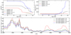 |
Fig. 2. Structure and spectra of exemplary clouds simulated with CLOUDY at constant pressure, assuming log(Ptot) = 16 cm−3 K, Vturb = 100 km s−1, Nc = 1024 cm−2 and Z = 10 Z⊙. The assumed values of ionizing fluxes are logΦ(H) = 18 cm−2 s−1 (displayed in green), 20 cm−2 s−1 (black) and 21 cm−2 s−1 (blue). An additional example with logΦ(H) = 18 cm−2 s−1 and the addition of extra mechanical heating is displayed in red. Top left: Cloud temperature profile in logarithmic scale as a function of depth (z) of the cloud. Top right: Cloud density profile in logarithmic scale as a function of depth (z) of the cloud. Bottom: Spectra of Fe II emission from different models, displayed with 100% covering factor. Each synthetic spectrum is broadened with a Gaussian kernel with FWHM = 2500 km s−1. |
For highly ionized clouds, the temperature drop across the cloud from the illuminated part towards its back is quite steep, accompanied by a rapid density increase, although the overall density difference between the two sides is only about 40%. In contrast, weakly ionized clouds exhibit a significant temperature drop across the cloud, while the density remains nearly constant throughout. These variations also affect the inward and outward spectra. For highly ionized clouds, the two spectra are relatively similar. However, for weakly ionized clouds, the outward radiation is much weaker, with the most substantial difference occurring in the UV part of the spectrum, which is significantly fainter compared to the illuminated side of the cloud.
When examining an even stronger ionizing flux, logΦ(H) = 21 cm−2 s−1, we do not observe a simple monotonic behaviour relative to the previous cases, and the temperature and density gradients across the cloud are steeper. Notably, at this higher ionization level, the physical conditions become less favourable for Fe II emission, resulting in a flux weaker than that seen in the logΦ(H) = 20 cm−2 s−1 case. For certain transitions in the UV and optical ranges, the flux is even lower than for the logΦ(H) = 18 cm−2 s−1 case.
When the predicted mechanical heating from the collision of clouds is included (H = 10−7 erg cm−3 s−1), the overall ionization level increases and the temperature gradient becomes shallower. However, this change is only evident in clouds exposed to weaker ionizing flux. The change in the temperature profile is only noticeable deep within the cloud, but on a linear scale, this would represent most of the cloud's body. Clouds exposed to stronger ionizing flux (logΦ(H) ≥ 20 cm−2 s−1) are unaffected by the presence of extra mechanical heating, as the impact of this heating is likely negligible. Consequently, the spectrum, the temperature, and density profiles of the clouds with logΦ(H) = 20–21 cm−2 s−1 are not displayed in Figure 2, since they remain unchanged compared to the cases without mechanical heating.
In contrast, for weakly ionized clouds, the presence of mechanical heating increases the temperature of the cloud's dark side relative to clouds without additional heating. This results in a noticeable increase in the emitted flux in the optical part of the spectrum, and consequently a potential reduction in Ropt. It is evident that the dark sides of clouds significantly contribute to the shape of the optical Fe II emission. This result is in agreement with previous studies suggesting that very low ionization lines, such as those of optical Fe II, originate from shielded regions (Joly 1987; Ferland & Persson 1989). Meanwhile, the interpretation of the UV spectrum is more complex due to the larger number of transitions and mechanisms involved (Wills et al. 1985).
4.2. The role of turbulent velocity in constant density and constant pressure approaches in simulations
Continuing with the assumption of constant pressure as detailed in Sect. 3.1, we compare clouds simulated with these conditions with those simulated under the assumption of constant density. Figure B.3. in Appendix B highlights the differences between these various simulations with similar physical conditions typically associated with the BLR. Two cases assume constant density, while the other two assume constant pressure. Additionally, we examine the impact of high turbulent velocity, Vturb = 100 km s−1, in one case for constant density and one for constant pressure.
In all scenarios, the clouds exhibit a complex temperature structure. However, the density is either constant or determined by the CLOUDY code under the condition of pressure equilibrium. This characteristic is directly linked to the role of turbulent velocity within the cloud. In the constant density scenario, for a given column density, the cloud size remains unchanged regardless of the turbulent velocity. In this case, increased turbulent velocity primarily enhances the gas emissivity without significantly altering the temperature or density profiles. In contrast, under constant pressure, turbulent velocity influences the temperature profile, which subsequently affects the density profile. As turbulent velocity increases, the density decreases and the cloud size expands for a fixed column density. Specifically, the diameter of the cloud increases by about two orders of magnitude in the presence of turbulent velocity.
The resulting spectra from these simulations are shown in the bottom panel of Figure B.3.. These spectra reveal that turbulent velocity plays a crucial role in shaping the Fe II emission. Notably, optical Fe II emission is not significantly produced in the absence of turbulent velocity under both constant density and constant pressure conditions. On the other hand, the shape of the Fe II profile changes very little for the same value of turbulent velocity, whether a constant pressure or constant density is imposed.
4.3. Fits of the three broad-band flux ratios without mechanical heating
We begin by analysing the first three global ratios (1) to (3) described in Sect. 3.3.
Using the computed grid and the measured fluxes for RM 102, we identify the parameters (total pressure and ionization flux) which best reproduce the observed value for each of the three ratios. An example plot, illustrating the parameter space of logΦ(H) and log(Ptot) under the conditions of Vturb = 0 km s−1 and Z=Z⊙, is presented in Figure 3. We assume equal contributions from the bright sides and the dark sides of clouds. Contour plots for various values of Ropt are shown, with the value measured in RM 102 highlighted by a solid red line. The dashed red line represents the contour corresponding to the 1-σ confidence range of the ratio. In Figure 3 both solid and dashed red lines are visible. When the solid red line is absent, the observed ratio is not reproduced within the selected parameter grid. Similarly, if the dashed red line is missing, the parameter grid does not reproduce the observed ratio within the 1-σ confidence interval. Additional plots are available at the link in Section Data availability.
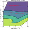 |
Fig. 3. Contour plots for the Ropt ratio described in Sect. 3.3 with constant Vturb = 0 km s−1, Z=Z⊙, and equal contributions from the bright sides and the dark sides of clouds. The position in the parameter space corresponding to the ratio measured in RM 102 is marked by a solid red line, while the dashed red line represents the 1-σ confidence range of the ratio. |
We summarize these findings by showing the plots for these three ratios in Figure 4. The lack of intersection between the red and blue lines indicates that a single density and ionization flux combination does not reproduce both RUV and the Ropt for RM 102. The observed overall RUV−opt only falls within the adopted grid when the density (or pressure) is very low. The range expands slightly when metallicity is increased to 20 times the solar value, but even then, the observed RUV is not reproduced. We can still identify the best solution (orange dot) in each of the contour plots which minimizes the χ2 fit for all these ratios. The lowest value of the χ2 in Figure 4 is 3.81, for 20 Z⊙.
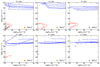 |
Fig. 4. Contour plots denoting the ratios observed in the source RM 102 for different values of metallicity and microturbulence. The black, red, and blue contours denote RUV−opt, RUV, and Ropt, respectively. An orange dot in each plot marks the position of the best χ2 for each bin of metallicity. |
We select the best solution for each metallicity value, and the best of all corresponds to the Z = 20 Z⊙, Vturb = 40 km s−1, logΦ(H) = 19.25 cm−2 s−1 and log(Ptot) = 14 cm−3 K (see first line in Table 4). For this solution we plot the modelled Fe II emission against the observed fluxes in RM 102 (see Figure A.1.). Using the observed flux, we still have the freedom to assume an arbitrary covering factor to match the data. We selected 0.24, as this value of f, for this solution, matches the integrated intensity of Fe II emission of RM 102 in the selected wavelength range. Such a covering factor is well within the expected range of the BLR covering factors, 0.1–0.3 (e.g. Peterson 2006; Collin et al. 2006; Panda 2021; see also Naddaf & Czerny 2024 for model-based estimates). Despite this formal acceptance, the actual representation of the Fe II emission is far from perfect. The UV data are marginally matched, but the optical emission is underproduced, particularly in the blue wing of the optical Fe II. Moreover, a strong emission feature that is absent in the observed spectrum is present at about 4300 Å. Other discrepancies include the lack of a dip in emission at approximately 2400 Å, and a significant underproduction of Fe II in the 3000–3500 Å range. The model predicts two clear spikes at approximately 2350 Å and ∼2610 Å, separated by a gap. This feature has been studied in previous works (Baldwin et al. 2004; Sarkar et al. 2021), and is discussed more in detail in Sect. 4.6. In the far UV, the same transitions appear in both the model and the data but with different intensities, suggesting that the physical conditions represented by the best-fit model do not yet fully reproduce the entire ionization balance in the medium.
When calculating the minimum χ2 for each metallicity bin, we notice that only the minimum χ2 associated with Z = 2 Z⊙ is departing significantly from the minimum χ2 solution observed at Z = 20 Z⊙. Indeed, only solutions with 5 Z⊙≤Z≤20 Z⊙ seem appropriate in the context of xA quasars (Panda et al. 2019b, 2020; Floris et al. 2024). Despite the large errors in the local subtraction of the underlying power-law, the fit is formally acceptable.
The overall consistency of the UV and optical emission in some specific ranges, assuming the predicted covering factor, is nonetheless notable given the adopted technique. However, the favoured ionization parameter logΦ(H) = 19.25 cm−2 s−1, is inconsistent with the observed SED of the object and the measured time delay of Hβ, as discussed in Pandey et al. (2024). Such high values of ionizing flux would require substantial internal shielding of the radiation emitted from the central engine, implying that the radiation received by the BLR clouds differs from the measured continuum emission. Under the favoured solution, the cloud density ranges from 3.27×107 cm−3 at the illuminated face to 3.60×108 cm−3 at the dark side. Such low densities are not typically associated with BLR conditions, suggesting that this solution may not be fully appropriate.
We also constructed similar contour plots (see Figure 5) for the case when 20% of the light came from the illuminated sides of the clouds and 80% from the dark sides, corresponding to A = 0.8. This configuration reflects a geometry where some clouds are obscured, such as in an inflow pattern (Horne et al. 2021). The new contour plots (see Figure 5) reveal some changes compared to the previous case, with the best fit found for a slightly different set of parameters (see Table 4), and a significantly reduced χ2 of 1.98. Table 3 presents the minimum χ2 results for each metallicity bin displayed in Figures 4 and 5. Table 3 further supports that the lowest χ2 values are obtained for a combination of high Z and a geometry where the dark sides of clouds are more represented than bright sides. Although the best χ2 results for both the 50–50 and 20–80 contributions are obtained with Z = 50 Z⊙, the only slight improvement in χ2 does not justify the dramatic increase in metallicity. Indeed, RM 102 does not exhibit extreme Fe II emission or an extreme L/LEdd which would be more commonly associated with extreme values of Z (Martínez-Aldama et al. 2018; Śniegowska et al. 2021; Floris et al. 2024). Therefore, we exclude the simulations with Z = 50 Z⊙ from Table 4 and favour a more physical solution of Z = 20 Z⊙.
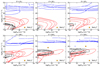 |
Fig. 5. Contour plots denoting the ratios observed in the source RM 102 for different values of metallicity and microturbulence, assuming 20% contribution from the bright side of the cloud and 80% from the dark side. The RUV−opt contours are shown in black, the RUV contours are shown in red, and the Ropt contours are shown in blue. The position associated with the best χ2 for each bin of metallicity is marked with an orange dot. |
Best solutions per Z bin.
Best fitting solutions
The model for the broad band is compared to the data in Figure A.1. in Appendix A. Although the UV Fe II emission nearly matches, some features in the UV region are not well represented, and the optical blue wing is strongly underproduced in the spectrum obtained from the CLOUDY simulations. Despite these issues, the improvement in χ2 compared to the previous case with equal contributions from both cloud sides is consistent with the enhancement in the overall shape of the template, even if it still does not fully represent the data. The physical conditions associated with this CLOUDY simulation appear more realistic than in the previous case, requiring less intense shielding from the central engine. Additionally, the cloud density in this scenario (nH∼109 cm−3) is still relatively low. While such low densities were once considered representative of the BLR, later studies suggested lower densities for high ionization lines and higher densities for low ionization lines like Hβ, Mg II and Fe II, starting from the end of the 1980s (Collin-Souffrin et al. 1988; Collin-Souffrin & Lasota 1988). Most of the recent works points towards much higher densities in the bulk of BLR (e.g. Panda et al. 2019b).
Low density values for the BLR clouds of RM 102 could be confirmed if a strong emission of C III]λ1909 were detected for the object, as C III] has a critical density of nc∼1010 cm−3 (Hamann et al. 2002). This line is clearly present in the composite quasar spectrum of Vanden Berk et al. (2001). Unfortunately, the SDSS spectrum of RM102 used in this work ends at ∼2000 Å. In addition, the C III] line might originate closer in than Fe II, as it is considered an intermediate line between low and high ionization lines (see e.g. Buendia-Rios et al. 2023).
4.4. Fits of the three broad band flux ratios with equivalent width control, without mechanical heating
To ensure sufficient Fe II flux while also accurately reflecting the observed ratios, we computed the χ2 value using a combination of the three ratios and the observed equivalent widths (EWs) of Fe II across the four considered spectral ranges under consideration. The values of the integrated Fe II fluxes used to calculate the EWs were scaled by a constant value of the covering factor f<1, according to Eq. (7). In this work, EWs are measured based on the incident continuum. Table 5 lists the observed Fe II EWs for the spectral ranges we have considered. For our analysis, we used the observed continuum and the observed Fe II flux. However, in our simulations, we employed the local incident continuum and the local emission as calculated by CLOUDY. In a plane-parallel geometry, the covering factor is set to 1, but we also consider arbitrary values of f to find the best match with the observations. The predicted EWs from CLOUDY simulations are compared by automatically selecting values of f that minimize the χ2. Figures uploaded on the Zenodo platform (see Section Data availability) show the EWs produced by an array of simulations with varying Z and Vturb. These figures separately display the EWs produced by the dark side spectrum, the illuminated side spectrum, and the total spectrum, specifically for the UV Fe II emission centred on Mg IIλ2800.
EW measurements of the regions of interest.
When assuming equal contributions from both the dark and bright sides of the cloud, the lowest χ2 value (χ2 = 7.15) was found with a parameter set similar to that of the equal contributions case without the EW control, albeit with slightly lower turbulence (see Table 4). In this scenario, the resulting f = 0.10 minimizes the χ2. When assuming unequal contributions from both sides, the minimum χ2 value obtained was 4.88, which, like the previous case, does not differ significantly from the initial solution that did not use EW control. The cloud density and temperature structure, as well as the Fe II templates associated with some of the best-fitting configurations listed in Table 4, are illustrated in Figure 6. For a relatively narrow range of Φ(H) values characterizing the best solutions, the temperature range is narrower than that in the general case (see Figure B.3.). However, this primarily affects the overall intensity of the Fe II emission rather than its spectral shape.
These results confirm that EW production is broadly in agreement with the trends of the observed ratios, and including EWs in the χ2 calculation does not drastically change the solutions. However, minimizing χ2 brings to a substantial underestimation of f with respect to the one obtained by measuring the integrated Fe II flux over the entire wavelength range (last column in Table 4) for all cases considered in Table 4. This discrepancy arises because the covering factor is a free parameter in the χ2 calculations with EW control. The most effective χ2 minimization prioritizes matching fluxes corresponding to the ratios with the smallest percentage errors, leaving substantial mismatches in the rest of the spectrum.
4.5. Solutions with mechanical heating
To investigate the potential contribution of mechanical heating from cloud collisions to the Fe II emission, we created a grid of CLOUDY simulations with logΦ(H) ranging from 17 to 22 cm−2 s−1 and constant pressure covering the log(Ptot) range of 14 to 18 cm−3 K. The adopted microturbulent velocity for all simulations is Vturb = 100 km s−1. The additional mechanical heating, as described in Sect. 3.2, is H = 10−7 erg cm−3 s−1. It is important to note, as discussed in Sect. 4.1, that mechanical heating significantly affects the cloud structure and emission only when the ionization flux is low. Figure B.1. displays a spectrum obtained from a simulation with mechanical heating, demonstrating the enhanced optical Fe II emission compared to the observed spectrum of our source.
Using the same approach to calculate the minimum χ2 from the first three flux ratios for this grid of simulations, and considering both equal and unequal contributions from the illuminated and dark sides of the clouds, we identified the best fits among all CLOUDY simulations performed in this study. As shown in Table 4, the two best solutions obtained using this method are very similar, with χ2 values of 1.44 and 1.45, respectively. The two solutions are also displayed in Figure A.3. and confronted with the observed Fe II emission from the source. The optimal solution is found with parameters of logΦ(H) ∼ 18.25 cm−2 s−1, log(Ptot) = 14.75 cm−3 K and Z=Z⊙. These remarkably low χ2 values, indicating a good statistical fit, require unexpectedly low ionizing flux. The Fe II emission region may be slightly farther from the central source than the location of Hβ, as discussed in Sect. 2, but not by a significant factor. Observed FWHM of the Fe II lines are only marginally narrower than those of Hβ (see Sect. 3.3), suggesting that the emitting region could be at most twice as distant, leading to a fourfold reduction in ionizing flux, as Φ(H) ∝  . However, the required reduction in ionizing flux in this case is by a factor of 150 compared to the ionizing flux received by Hβ (Φ(H) = 20.43 cm−2 s−1, as listed in Table 1).
It is possible that the BLR region does not receive the same radiation as the observer, with this discrepancy resulting from shielding, where radiation is attenuated by an intervening medium between the nuclear emission source and the Fe II region. The required optical depth to achieve a photon reduction by a factor of 150 would be of the order of τ = 5. Nevertheless, the extreme Fe II emission observed on the red side of Mg II in both solutions displayed in Figure A.3. makes these best solutions with mechanical heating not compatible with the observed Fe II emission from the source.
The combination of high microturbulence and mechanical heating efficiently produces Fe II emission, requiring a relatively low covering factor to match observed values, even when measured against the unabsorbed continuum. The significant role of mechanical heating has been proposed in early studies addressing the iron emission problem in AGNs (Grandi 1981; Joly 1987; Ferland & Persson 1989; Joly et al. 2007). These models consistently require relatively low covering factor, as was also demonstrated by Joly et al. (2007). Earlier studies emphasized the necessity of high local cloud density, collisional heating, high column density, and shielding from the central source to explain iron emission, but the problem remains not fully solved.
4.6. Contribution from individual transitions
In Sect. 4.3, we demonstrated that the solutions obtained by considering the first three flux ratios do not fully reproduce the observed spectrum when using the adopted covering factors. Several spectral features exhibited significant discrepancies between the observed data and the model, affecting the shape of the emission template. In this section, we delve deeper into these discrepancies by examining the intensities of specific transitions as functions of the simulation parameters.
Following the work of Kovačević-Dojčinović & Popović (2015) and Popović et al. (2019), we focus on UV multiplets 60, 61, 62, 63, 78, along with two empirical transitions observed in the I Zw 1 UV spectrum from Popović et al. (2019). These transitions were centred at 2720 Å and 2840 Å, respectively, which we refer to as IZw1a and IZw1b. Popović et al. (2019) suggested that these transitions likely originate from high excitation levels not included in their study. However, these transitions are correctly incorporated in the CLOUDY simulations used here and are present in the spectra generated with our preferred set of parameters outlined in Section 4.3. Additionally, we analyse the spike-to-gap ratio, a key diagnostic of plasma conditions (Baldwin et al. 2004; Sarkar et al. 2021). The specific spectral ranges associated with each of these transitions are described in Table 6.
UV Fe II lines.
To improve the template fits, we incorporated intensity ratios of these specific transitions into the χ2 computation, using them as diagnostics to refine the accuracy of our models. These ratios, which we refer to as the Spike-to-spike ratio, the Spike-to-gap ratio (Sarkar et al. 2021), R2800 and R2900, are listed in Table 7 along with their observed values in the spectrum of RM 102.
UV Fe II line ratios measured in the spectrum of RM 102.
After including these additional ratios to the χ2 calculation, the best-fitting model, with χ2 = 7.97, corresponds to a reasonable set of parameters: logΦ(H) = 20 cm−2 s−1, log(Ptot) = 16 cm−3 K, Vturb = 100 km s−1 and Z = 20 Z⊙. This model assumes unequal contributions from the bright and dark sides of the cloud. The spectrum produced by this simulation is shown in Figure B.2.. Although the χ2 value increases slightly when including the four additional ratios, the match with the observed data does not deteriorate. On the contrary, the template generated from this specific simulation, using the covering factor detailed in Table 4, aligns closely with most of the features observed in the original spectrum of RM 102. The primary exceptions are of the two strong spikes associated with the spike-to-spike and the spike-to-gap ratios, which strongly increase in intensity with higher metallicities (see the online content in Section Data availability), and the features at 4350 Å as well as the weaker optical blue wing of Fe II. Despite these discrepancies, this simulation represents our preferred solution because it achieves a good balance between fitting the observed data and maintaining a physically plausible set of parameters, requiring minimal shielding and suggesting a cloud density of nH∼109 cm−3.
The contour plots for the additional ratios, together with the discussion on their trends, have been uploaded on the Zenodo platform (see Section Data availability). Interestingly, our constant pressure analysis of the spike-to-gap ratio favours the turbulent velocity of 40 km s−1 (consistent with the requirement for three basic ratios) but indicates a lower metallicity, solar to 5 times solar.
5. Discussion
In this study, we modelled the Fe II contribution to the emission of RM 102, a quasar that is highly representative of the general quasar population as well as xA sources as shown in Figure 1. Our model comprehensively covers both the UV and optical bands, utilizing the latest atomic data available in the current version of CLOUDY (Chatzikos et al. 2023) and incorporating all available transitions. The modelling was based on the assumption of constant pressure, which is more appropriate for maintaining cloud stability. We explored a broad range of parameters, including ionization flux, total pressure, metallicity, and turbulent velocity. Additionally, we considered the effects of mechanical heating and the geometrical enhancement of the contribution from the dark sides of the clouds to the total spectrum. The most relevant fits are summarized in Table 4. There, the Fe II emission is measured with respect to the incident continuum assumed in the model.
Although our simulations do not fully reproduce the observed spectrum, they allow us to draw several tentative conclusions, which are discussed below.
5.1. Constant density versus constant pressure
Clouds not in hydrostatic equilibrium would be destroyed on a dynamical timescale due to pressure gradients. Such gradients are expected in constant density clouds exposed to strong irradiation from one side. Consequently, it is generally recommended to model cloud interior structures under the assumption of pressure equilibrium (Begelman & McKee 1990; Adhikari et al. 2018; Stern et al. 2014; Netzer et al. 2024). This is a key distinction from the approach of Pandey et al. (2024), which assumes constant density clouds. In Sect. 4.2, we discussed the role of turbulent velocity in both constant pressure and constant density simulations. Turbulent velocity, along with metallicity, significantly influences the parameter space of Φ(H) and Ptot, as observed in the contour plots in Figures 4 and 5. However, the constant pressure assumption more effectively captures the variations in the physical conditions of the gas driven by changes in metallicity and turbulent velocity. This approach allows the observed ratios to explore a broader range of the parameter space. Incorporating turbulent velocity ultimately leads to larger cloud sizes and more complex cloud structures. In the extreme case of very high turbulence, the turbulence term pressure dominates the pressure balance, reducing the differences between the constant pressure and the constant density assumptions. However, future studies that incorporate multi-zone emission regions should prioritize the constant pressure assumption, as turbulence may not always reach such high levels in all scenarios.
5.2. Consistency of the required and observed Φ(H), and the potential need for shielding
The apparent overproduction of the Fe II UV emission in our models might be due to inaccuracies in determining the underlying continuum. This issue could stem from confusion with pseudocontinua, reddening effects, or contributions from starlight. The mean slope of the spectrum above ∼5000 Å is 2.08, which is only slightly flatter than the slope of 2.33 expected from a standard accretion disk (Shakura & Sunyaev 1973). This flattening is likely due to starlight contribution, as RM 102 is not particularly luminous, with a black hole mass just above 108 M⊙. The modest luminosity leaves little room for significant internal reddening.
We also explored the possibility of reddening by examining the Balmer decrement. Although the higher-order Balmer lines are clearly visible in the spectrum, the line ratios are quite uncertain (see Table 8). This uncertainty is likely because Balmer line ratios are sensitive to both the density and temperature of the clouds, as indicated by both simulations and observational data (Ilić et al. 2012). Nevertheless, the observed ratios are consistent with theoretical expectations (Osterbrock 1989) and with the typical values for AGN as reported in Popović (2003). This consistency supports the conclusion that the disk emission in RM 102 is not significantly affected by intrinsic reddening.
Balmer decrement in RM 102.
Performed computations did not rely on the precise distance measurement from the SMBH to the BLR. However, this distance, inferred from the time delay between the continuum and line emissions, has been estimated and is reported in Table 1. This delay implies a specific value for the ionizing flux. We observe that the solutions presented in Table 4 do not fully satisfy this condition, with some deviating significantly from the values based on the observed continuum and the measured time delay. This discrepancy could imply that the net time delay does not accurately reflect the distribution of the flux within the source, or that the BLR actually experiences a different incident continuum than the one observed, potentially due to some form of obscuration. Both effects could be significant, but the substantial mismatch between the measured and modelled values of Φ(H) is concerning, particularly since the FWHMs of the Fe II and Hβ lines are very similar, as discussed in Sect. 4.5. It is challenging to disentangle these effects reliably.
Without a precise distance, we cannot scale the model to the data in absolute units. If we assume the delay provides the correct distance, then the strength of the features (effectively, the covering factor) reported in Table 4 should be rescaled to match the observed continuum by accounting for the difference in assumed and observed Φ(H). This adjustment would immediately favour the last two models, which are closest to the observationally inferred Φ(H).
With the exception of the best solutions obtained with the addition of mechanical heating in the simulations, most of the best solutions found in this work (see Table 4) require only marginal shielding relative to the measured value of logΦ(H) ∼ 20.5 cm−2 s−1 of our source. This consistency is noteworthy, as it suggests that substantial shielding is not necessary for our favoured model, which minimizes χ2 by considering all ratios and assumes a 20% contribution from the bright side and an 80% contribution from the dark side of the cloud.
5.3. Are dark sides of clouds favoured?
Comparing the contours in Figure 5 with those in Figure 4 suggests a strong preference for an inflow pattern geometry, where the dark sides of the clouds are disproportionately represented compared to their illuminated sides. As a matter of fact, the contours associated with the three ratios described in Sect. 3.3 are more consistently produced, and overlap more under the assumption that Fe II emission preferentially comes from the dark sides of clouds (see also Panda et al. 2018) rather than equally from both sides. Assuming Vturb∼100 km s−1 (non-thermal turbulence, consistent with the chaotic motion of clouds), we find that although the contours do not perfectly overlap, this configuration provides the best fit. It maintains reasonable physical conditions that align with both our models and observations. The optical ratio still tends towards higher values of Φ(H); however, within error, these ratios can be consistent with canonical parameters associated with the physical conditions of the BLR (Netzer 2013, 2020), or potentially with slightly higher values of Vturb.
It is noteworthy that, although the microturbulence parameter cannot be directly measured in the source, Vturb∼100 km s−1 is not extreme and has been adopted in previous studies (Panda et al. 2018, 2019a; Sarkar et al. 2021; Panda 2021; Pandey et al. 2024). Slightly higher values of Vturb could potentially reconcile all three ratios together, though a combination with high Z could potentially lead to significant overproduction of Fe II emission.
In conclusion, when comparing the contours in Figures 4 and 5, the difference is striking. Using only the first three diagnostic ratios studied in Sect. 4.3, it is evident that the only way to reproduce physical conditions consistent with the observed Φ(H) and appropriate density values for the BLR, is assuming Z∼20 Z⊙, Vturb∼100 km s−1 and a geometry that favours dark sides. This trend is also observed when considering all the additional ratios discussed in Section 4.6.
5.4. The role of mechanical heating in the BLR
Mechanical heating does improve the best χ2 with just a handful of simulations needed. The best χ2 values found are associated with simulations featuring Φ(H) levels that are formally incompatible with the observations of RM 102.
These simulations would require extreme levels of internal reddening or shielding. In this work, we included mechanical heating but considered only the drop in the ionizing flux, neglecting the (likely highly significant) spectral changes caused by shielding. Consequently, these models require further, more sophisticated simulations to evaluate their applicability to the studied source.
5.5. Model constraints for the density, turbulence, and metallicity
All the best-fit solutions presented in Table 4 indicate a general trend of average nH∼109 cm−3, with the exception of the solution with log(Ptot) = 18 cm−3 K, which exhibits a higher density of nH∼1011 cm−3. Solutions derived using the minimum χ2 method strongly favour a condition of nH≈109 cm−3 in the BLR. These lower density values for RM 102 could be further validated by measuring the intensity of the C III] emission, which is not present in the spectrum used in this study. There is also a consistent trend in the preferred solutions regarding microturbulence, with Vturb∼100 km s−1. The metallicity is expected to lie within the range of 5 Z⊙≤Z≤20 Z⊙. Solutions with higher metallicity are not consistent with our findings for this source and are thus excluded.
5.6. Multiple emission regions
A single cloud approximation does not perfectly match the overall spectrum of RM 102. It was frequently suggested that optical and UV Fe II emission originate from two distinct regions (Baldwin et al. 2004; Gaskell et al. 2022). Some correlation between the two regions is observed (e.g. Kovačević-Dojčinović & Popović 2015; Panda et al. 2019a), and the measured time delays of the optical and UV emission are not significantly different as shown by Zajaček et al. (2024). However, the significant average redshift in the UV Fe II lines, which is not seen in the optical UV counterparts, suggests an outflow component predominantly affecting the UV region (Kovačević-Dojčinović & Popović 2015). Additionally, Gaskell et al. (2022) suggests that the optical Fe II is subject to considerable reddening, which is not observed in the UV Fe II emission. Given these discrepancies, we tested whether allowing for two distinct types of clouds could improve the representation of the data.
To explore this hypothesis, we combined emissions from two clouds and calculated the minimum χ2 among all combinations of simulations, as described in Sect. 3.3, but extended to two clouds. Despite these efforts, all solutions converged back to a single-cloud model, reproducing the results obtained for scenarios where both the bright and dark sides of the clouds contributed equally and for scenarios emphasizing dark side emissions. Thus, no combination of simulations appears to enhance the single-cloud interpretation.
This approach, however, does not fully address the common mismatch between optical and UV observational templates that are applied to the same sources with different normalizations. In reality, no simulation achieves a perfect optical shape and intensity while simultaneously producing no UV emission, or vice versa for the optical range. Consequently, models that consider only optical or only UV emissions as originating from two physically distinct regions cannot provide a complete solution because the radiation from each region inevitably affects the other band. Typically, our simulations generate similar amounts of UV emission but show wide variation in the optical range, especially when additional heating is included. Conversely, the ability of Fe II observational templates based on IZw1 to fit the spectra of most quasars remains unexplained, while theoretical templates fail to match the optical wavelength range when typical BLR physical conditions are assumed (Gaskell et al. 2022; Zhang et al. 2024).
This is likely to be the case for any multi-zone modelling approach, such as the locally optimized cloud (LOC) model proposed by Baldwin et al. (1995) or any Monte Carlo-type approach combining multiple emitting regions. Specifically, spectral features that are not well-modelled by any single solution, despite representing a broad parameter space, are unlikely to be accurately reproduced by combining multiple solutions. Figure 7 illustrates this issue. The upper panel shows Fe II models derived from equal contributions from the dark and bright sides of the clouds, while the lower panel illustrates models for 80% dark-side and 20% bright-side contributions. Any LOC model would essentially combine these contributions. However, some spectral ranges remain poorly represented. The most significant discrepancy lies in the blue portion of the optical Fe II emission. All models under-predict the observed features in this region, and any enhancement of this emission inevitably overproduces the red optical emission and dramatically amplifies the UV emission.
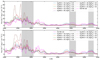 |
Fig. 7. Top: Spectra of the Fe II emission obtained for several simulations in the Z = 20 Z⊙ and Vturb = 100 km s−1 grid. Grey-shaded regions indicate spectral ranges used to compute RUV and Ropt. Each template is normalized by the f parameter to match the integrated flux of the RM 102 spectrum in the 2000–5500 Å range. The figure demonstrates that no simulation accurately reproduces the observed Fe II emission across all grey-marked regions. Synthetic spectra are broadened using a Gaussian kernel with FWHM = 2500 km s−1. Bottom: Same as the top figure, but for 20% contribution from the bright side and 80% from the dark side. |
Kinematic studies of UV and optical emission, along with time-delay measurements, imply subtle differences between the two regions (e.g. Kovačević-Dojčinović & Popović 2015; Le & Woo 2019; Prince et al. 2023), with similar distances and complex dynamics overall. Further investigations, particularly those incorporating the spectral effects of shielding, are essential and may prove crucial for resolving these challenges.
5.7. Disk winds possibly shielding the bright sides
The predominance of emission from the dark sides of the clouds suggests that there may be some form of shielding preventing the bright sides, which are located further from the observer and behind the black hole, from significantly contributing to the observed spectrum. A similar effect has been observed in reverberation mapping studies of certain sources, where the response function peaks at the shortest possible time delay, close to the observer's line of sight. In these cases, a second peak associated with the bright sides is present but shows a much-reduced amplitude (see e.g. Horne et al. 2021, for NGC 5548). However, we do not observe substantial reddening of the disk in RM 102, as the spectral slope is roughly consistent with that of a standard accretion disk (see Sect. 3.3). Attempts to introduce intrinsic reddening using the extinction law from Czerny et al. (2004) did not improve the spectral fit, indicating that any medium shielding the bright sides is likely dust-free and highly ionized.
Such a medium could plausibly be in the form of magnetically driven winds that originate close to the black hole (e.g. Fukumura et al. 2024, and the references therein). These outflows are challenging to detect directly, but there is observational evidence of ultra-fast outflows (UFOs) with velocities ranging from 0.03 to 0.6 times the speed of light. These UFOs are detected through shifts in the emission lines of highly ionized species in the X-ray band (e.g. Gianolli et al. 2024). The existence of such winds could provide a natural explanation for the observed shielding effects.
5.8. A comment on the current state of atomic transitions
Some observed spectral features, such as the dip near 2400 Å and the additional feature around 4350 Å, are not reproduced in our models. CLOUDY offers various atomic databases for use in simulations, and the differences between these databases have been discussed by Sarkar et al. (2021). For this study, we utilized the Fe II database from Smyth et al. (2019), as recommended by Sarkar et al. (2021). This database is now the default in CLOUDY and includes a comprehensive set of atomic data, representing the most advanced modelling currently available. However, the discrepancies between predicted and observed features suggest that there is still significant room for improvement in the atomic data and modelling techniques. Even solutions that assume shielding and incorporate mechanical heating fail to fully replicate the observed spectral features, despite providing better agreement with measured flux ratios.
Additionally, the methods used to solve the radiative transfer equations may contribute to these discrepancies. Netzer (2020) pointed out that current photoionization codes using the escape probability formalism often fail to accurately compute transitions in relatively dense, optically thick clouds. While alternative codes such as TITAN (Dumont et al. 2000, 2003) and TLUSTY (Hubeny et al. 2000) exist, they lag behind CLOUDY in terms of the richness of their atomic data, even in their most recent versions (e.g. Palit et al. 2024). This highlights the need for further development in both atomic databases and radiative transfer methodologies to enhance the accuracy of modelling complex astrophysical environments.
6. Conclusions
After analysing the Fe II emission of the bright quasar RM 102 employing a range of techniques and assumptions, we draw several key conclusions.
-
–
We find strong evidence supporting the predominance of the dark sides of clouds over isotropic emission for photoionization-driven emission models. This finding aligns with previous studies on the Hβ profile using reverberation mapping (Horne et al. 2021). The similarity in the FWHM of the Fe II lines and Hβ confirms that Fe II originates from the same regions as Hβ (albeit a slightly more extended one), underscoring the critical role of dark sides in Fe II emission. This predominance is crucial for matching the observed RUV−opt ratios and the RUV ratios in the Φ(H)-nH parameter space compatible with the expected physical conditions in the BLR (Gaskell et al. 2022) and the observations of RM 102.
-
–
Our results indicate significant chemical enrichment in the BLR of RM 102. Combined with high turbulent velocities and the predominance of dark sides, this enrichment creates the necessary conditions to produce most of the observed Fe II emission ratios. The high metallicity inferred from our models is consistent with findings from similar studies of other quasars (Nagao et al. 2006; Martínez-Aldama et al. 2018; Maiolino & Mannucci 2019; Panda et al. 2019b; Śniegowska et al. 2021; Panda 2021; Garnica et al. 2022; Floris et al. 2024).
-
–
The favoured solution described in Sect. 4.6 with the minimum χ2 result, of logΦ(H) = 20 cm−2 s−1, Z = 20 Z⊙, log(Ptot) = 16 cm−3 K and Vturb = 100 km s−1, aligns well with the measured Φ(H) from RM 102. This solution also supports the presence of low-density (nH∼109 cm−3) BLR clouds. Although this density is lower than typical values for BLR clouds, observations of C III] intensity with instruments such as X-Shooter at the Very Large Telescope (VLT) could provide further insight into the low density observed and help refine these constraints.
-
–
The best χ2 results were obtained with models incorporating strong shielding and mechanical heating. However, these models were not derived self-consistently, as the spectral impact of the shielding material was not fully considered. Future work must include assumptions about the nature and ionization state of the obscurer to achieve self-consistent results.
-
–
While some discrepancies in observed Fe II features might suggest multiple emission regions, our study found no compelling evidence to support this hypothesis. Further analysis using more advanced multi-zone modelling approaches, such as the locally optimized cloud (LOC) method (Baldwin et al. 1995) or Monte Carlo-type simulations, could offer additional insights into this possibility.
-
–
The absence of specific Fe II features in the observed spectra of RM 102, as well as the appearance of additional features in the simulations (such as the emission at 4350 Å), along with notable discrepancies in the intensity of specific lines, highlight potential limitations in the atomic data used in CLOUDY. Despite being one of the most comprehensive spectral synthesis codes, there may be missing transitions or inaccuracies in transition rates affecting the modelling of Fe II emission. Further research on Fe II emission is necessary to address these gaps.
Data availability
The trends associated with the Fe II line ratios and their discussion have been uploaded on the Zenodo2 platform, together with the trends associated with the EW production. Plots of their behaviour in different physical conditions of microturbulence and contribution from the different sides of the clouds are displayed.
Acknowledgments
We thank the anonymous referee for constructive comments and suggestions that helped improve the manuscript. This project has received funding from the European Research Council (ERC) under the European Union's Horizon 2020 research and innovation program (grant agreement No. [951549]). BC acknowledges the OPUS-LAP/GA CR-LA bilateral project (2021/43/I/ST9/01352/OPUS 22 and GF23-04053L). AF acknowledges financial support from the Center for Theoretical Physics, Polish Academy of Sciences during his stay in Warsaw. AP acknowledges funding from the Chinese Academy of Sciences President's International Fellowship Initiative (PIFI), Grant No. 2024PVC0088. MLM-A acknowledges financial support from Millenium Nucleus NCN2023_002 (TITANs) and ANID Millennium Science Initiative (AIM23-0001). SP acknowledges the financial support of the Conselho Nacional de Desenvolvimento Científico e Tecnológico (CNPq) Fellowship 301628/2024-6 and is supported by the international Gemini Observatory, a program of NSF NOIRLab, which is managed by the Association of Universities for Research in Astronomy (AURA) under a cooperative agreement with the U.S. National Science Foundation, on behalf of the Gemini partnership of Argentina, Brazil, Canada, Chile, the Republic of Korea, and the United States of America. AF was funded by the European Union ERC-2022-STG – BOOTES – 101076343. Views and opinions expressed are however those of the author(s) only and do not necessarily reflect those of the European Union or the European Research Council Executive Agency. Neither the European Union nor the granting authority can be held responsible for them.
References
- Adhikari, T. P., Hryniewicz, K., Różańska, A., Czerny, B., & Ferland, G. J. 2018, ApJ, 856, 78 [NASA ADS] [CrossRef] [Google Scholar]
- Baldwin, J., Ferland, G., Korista, K., & Verner, D. 1995, ApJ, 455, L119 [NASA ADS] [Google Scholar]
- Baldwin, J. A., Ferland, G. J., Korista, K. T., Hamann, F., & LaCluyzé, A. 2004, ApJ, 615, 610 [NASA ADS] [CrossRef] [Google Scholar]
- Barth, A. J., Pancoast, A., Bennert, V. N., et al. 2013, ApJ, 769, 128 [NASA ADS] [CrossRef] [Google Scholar]
- Begelman, M. C., & McKee, C. F. 1990, ApJ, 358, 375 [NASA ADS] [CrossRef] [Google Scholar]
- Borkar, A., Adhikari, T. P., Różańska, A., et al. 2021, MNRAS, 500, 3536 [Google Scholar]
- Boroson, T. A., & Green, R. F. 1992, ApJS, 80, 109 [Google Scholar]
- Bruhweiler, F., & Verner, E. 2008, ApJ, 675, 83 [NASA ADS] [CrossRef] [Google Scholar]
- Buendia-Rios, T. M., Negrete, C. A., Marziani, P., & Dultzin, D. 2023, A&A, 669, A135 [NASA ADS] [CrossRef] [EDP Sciences] [Google Scholar]
- Cardelli, J. A., Clayton, G. C., & Mathis, J. S. 1989, ApJ, 345, 245 [Google Scholar]
- Chatzikos, M., Bianchi, S., Camilloni, F., et al. 2023, Rev. Mex. Astron. Astrofis., 59, 327 [Google Scholar]
- Collin, S., Kawaguchi, T., Peterson, B. M., & Vestergaard, M. 2006, A&A, 456, 75 [NASA ADS] [CrossRef] [EDP Sciences] [Google Scholar]
- Collin-Souffrin, S., & Lasota, J. -P. 1988, PASP, 100, 1041 [NASA ADS] [CrossRef] [Google Scholar]
- Collin-Souffrin, S., Joly, M., Heidmann, N., & Dumont, S. 1979, A&A, 72, 293 [NASA ADS] [Google Scholar]
- Collin-Souffrin, S., Dyson, J. E., McDowell, J. C., & Perry, J. J. 1988, MNRAS, 232, 539 [NASA ADS] [CrossRef] [Google Scholar]
- Czerny, B., Li, J., Loska, Z., & Szczerba, R. 2004, MNRAS, 348, L54 [NASA ADS] [CrossRef] [Google Scholar]
- Czerny, B., Chevallier, L., Gonçalves, A. C., Różańska, A., & Dumont, A. M. 2009, A&A, 499, 349 [NASA ADS] [CrossRef] [EDP Sciences] [Google Scholar]
- Du, P., Wang, J. -M., Hu, C., et al. 2016, ApJ, 818, L14 [NASA ADS] [CrossRef] [Google Scholar]
- Dumont, A. M., Abrassart, A., & Collin, S. 2000, A&A, 357, 823 [NASA ADS] [Google Scholar]
- Dumont, A. M., Collin, S., Paletou, F., et al. 2003, A&A, 407, 13 [NASA ADS] [CrossRef] [EDP Sciences] [Google Scholar]
- Ferland, G. J., & Elitzur, M. 1984, ApJ, 285, L11 [Google Scholar]
- Ferland, G. J., & Persson, S. E. 1989, ApJ, 347, 656 [NASA ADS] [CrossRef] [Google Scholar]
- Floris, A., Marziani, P., Panda, S., et al. 2024, A&A, 689, A321 [NASA ADS] [CrossRef] [EDP Sciences] [Google Scholar]
- Fukumura, K., Mehdipour, M., Behar, E., et al. 2024, arXiv e-prints [arXiv:arXiv:2403.07086] [Google Scholar]
- Garnica, K., Negrete, C. A., Marziani, P., et al. 2022, A&A, 667, A105 [NASA ADS] [CrossRef] [EDP Sciences] [Google Scholar]
- Gaskell, M., Thakur, N., Tian, B., & Saravanan, A. 2022, Astron. Nachr., 343, e210112 [NASA ADS] [CrossRef] [Google Scholar]
- Gianolli, V. E., Bianchi, S., Petrucci, P. -O., et al. 2024, A&A, 687, A235 [NASA ADS] [CrossRef] [EDP Sciences] [Google Scholar]
- Gonçalves, A. C., Collin, S., Dumont, A. M., et al. 2006, A&A, 451, L23 [NASA ADS] [CrossRef] [EDP Sciences] [Google Scholar]
- Grandi, S. A. 1981, ApJ, 251, 451 [Google Scholar]
- Guo, H., Shen, Y., & Wang, S. 2018, Astrophysics Source Code Library [record ascl:1809.008] [Google Scholar]
- Hamann, F., Korista, K. T., Ferland, G. J., Warner, C., & Baldwin, J. 2002, ApJ, 564, 592 [NASA ADS] [CrossRef] [Google Scholar]
- He, Z., Jiang, N., Wang, T., et al. 2021, ApJ, 907, L29 [NASA ADS] [CrossRef] [Google Scholar]
- Horne, K., De Rosa, G., Peterson, B. M., et al. 2021, ApJ, 907, 76 [Google Scholar]
- Hu, C., Du, P., Lu, K. -X., et al. 2015, ApJ, 804, 138 [NASA ADS] [CrossRef] [Google Scholar]
- Hu, C., Li, Y. -R., Du, P., et al. 2020, ApJ, 890, 71 [NASA ADS] [CrossRef] [Google Scholar]
- Hubeny, I., Agol, E., Blaes, O., & Krolik, J. H. 2000, ApJ, 533, 710 [NASA ADS] [CrossRef] [Google Scholar]
- Ilić, D., Popović, L. Č., La Mura, G., Ciroi, S., & Rafanelli, P. 2012, A&A, 543, A142 [NASA ADS] [CrossRef] [EDP Sciences] [Google Scholar]
- Joly, M. 1987, A&A, 184, 33 [NASA ADS] [Google Scholar]
- Joly, M., Véron-Cetty, M., & Véron, P. 2007, in The Central Engine of Active Galactic Nuclei, eds. L. C. Ho, & J. W. Wang, ASP Conf. Ser., 373, 376 [Google Scholar]
- Joly, M., Véron-Cetty, M., & Véron, P. 2008, in Rev. Mex. Astron. Astrofis. Conf. Ser., 32, 59 [Google Scholar]
- Kovačević-Dojčinović, J., & Popović, L. Č. 2015, ApJS, 221, 35 [Google Scholar]
- Kovačević-Dojčinović, J., Marčeta-Mandić, S., & Popović, L. Č. 2017, Front. Astron. Space Sci., 4, 7 [Google Scholar]
- Le, H. A. N., & Woo, J. -H. 2019, ApJ, 887, 236 [NASA ADS] [CrossRef] [Google Scholar]
- Lu, K. -X., Wang, J. -G., Zhang, Z. -X., et al. 2021, ApJ, 918, 50 [NASA ADS] [CrossRef] [Google Scholar]
- Maiolino, R., & Mannucci, F. 2019, A&A Rev., 27, 3 [NASA ADS] [CrossRef] [Google Scholar]
- Martínez-Aldama, M. L., del Olmo, A., Marziani, P., et al. 2018, A&A, 618, A179 [NASA ADS] [CrossRef] [EDP Sciences] [Google Scholar]
- Marziani, P., Sulentic, J. W., Zwitter, T., Dultzin-Hacyan, D., & Calvani, M. 2001, ApJ, 558, 553 [NASA ADS] [CrossRef] [Google Scholar]
- Marziani, P., Sulentic, J. W., Stirpe, G. M., Zamfir, S., & Calvani, M. 2009, A&A, 495, 83 [NASA ADS] [CrossRef] [EDP Sciences] [Google Scholar]
- Marziani, P., Dultzin, D., Sulentic, J. W., et al. 2018, Front. Astron. Space Sci., 5, 6 [CrossRef] [Google Scholar]
- Mathews, W. G., & Ferland, G. J. 1987, ApJ, 323, 456 [NASA ADS] [CrossRef] [Google Scholar]
- Müller, A. L., Naddaf, M. -H., Zajaček, M., et al. 2022, ApJ, 931, 39 [CrossRef] [Google Scholar]
- Naddaf, M. -H., & Czerny, B. 2024, Universe, 10, 29 [Google Scholar]
- Naddaf, M. -H., Czerny, B., & Szczerba, R. 2021, ApJ, 920, 30 [NASA ADS] [CrossRef] [Google Scholar]
- Nagao, T., Marconi, A., & Maiolino, R. 2006, A&A, 447, 157 [NASA ADS] [CrossRef] [EDP Sciences] [Google Scholar]
- Netzer, H. 2013, The Physics and Evolution of Active Galactic Nuclei (Cambridge University Press) [Google Scholar]
- Netzer, H. 2020, MNRAS, 494, 1611 [NASA ADS] [CrossRef] [Google Scholar]
- Netzer, H., Goad, M. R., Barth, A. J., et al. 2024, arXiv e-prints [arXiv:arXiv:2410.02652] [Google Scholar]
- Osterbrock, D. E. 1989, Ann. New York Acad. Sci., 571, 99 [Google Scholar]
- Palit, B., Różańska, A., Petrucci, P. O., et al. 2024, A&A, 690, A308 [NASA ADS] [CrossRef] [EDP Sciences] [Google Scholar]
- Panda, S. 2021, A&A, 650, A154 [NASA ADS] [CrossRef] [EDP Sciences] [Google Scholar]
- Panda, S., Czerny, B., Adhikari, T. P., et al. 2018, ApJ, 866, 115 [CrossRef] [Google Scholar]
- Panda, S., Czerny, B., Done, C., & Kubota, A. 2019a, ApJ, 875, 133 [CrossRef] [Google Scholar]
- Panda, S., Marziani, P., & Czerny, B. 2019b, ApJ, 882, 79 [NASA ADS] [CrossRef] [Google Scholar]
- Panda, S., Martínez-Aldama, M. L., Marinello, M., et al. 2020, ApJ, 902, 76 [NASA ADS] [CrossRef] [Google Scholar]
- Pandey, A., Martínez-Aldama, M. L., Czerny, B., et al. 2024, arXiv e-prints [arXiv:arXiv:2401.18052] [Google Scholar]
- Peterson, B. M. 2006, in Physics of Active Galactic Nuclei at all Scales, ed. D. Alloin, 693, 77 [NASA ADS] [CrossRef] [Google Scholar]
- Popović, L. Č. 2003, ApJ, 599, 140 [CrossRef] [Google Scholar]
- Popović, L. Č., Kovačević-Dojčinović, J., & Marčeta-Mandić, S. 2019, MNRAS, 484, 3180 [Google Scholar]
- Prince, R., Zajaček, M., Panda, S., et al. 2023, A&A, 678, A189 [NASA ADS] [CrossRef] [EDP Sciences] [Google Scholar]
- Salviander, S., Shields, G. A., Gebhardt, K., & Bonning, E. W. 2007, ApJ, 662, 131 [NASA ADS] [CrossRef] [Google Scholar]
- Sargent, W. L. W. 1968, ApJ, 152, L31 [NASA ADS] [CrossRef] [Google Scholar]
- Sarkar, A., Ferland, G. J., Chatzikos, M., et al. 2021, ApJ, 907, 12 [NASA ADS] [CrossRef] [Google Scholar]
- Shakura, N. I., & Sunyaev, R. A. 1973, A&A, 24, 337 [NASA ADS] [Google Scholar]
- Shapovalova, A. I., Popović, L. Č., Burenkov, A. N., et al. 2012, ApJS, 202, 10 [NASA ADS] [CrossRef] [Google Scholar]
- Shen, Y., Hall, P. B., Horne, K., et al. 2019, ApJS, 241, 34 [NASA ADS] [CrossRef] [Google Scholar]
- Shen, Y., Grier, C. J., Horne, K., et al. 2023, arXiv e-prints [arXiv:arXiv:2305.01014] [Google Scholar]
- Smyth, R. T., Ramsbottom, C. A., Keenan, F. P., Ferland, G. J., & Ballance, C. P. 2019, MNRAS, 483, 654 [NASA ADS] [CrossRef] [Google Scholar]
- Śniegowska, M., Marziani, P., Czerny, B., et al. 2021, ApJ, 910, 115 [CrossRef] [Google Scholar]
- Stern, J., Laor, A., & Baskin, A. 2014, MNRAS, 438, 901 [NASA ADS] [CrossRef] [Google Scholar]
- Sulentic, J. W., Zwitter, T., Marziani, P., & Dultzin-Hacyan, D. 2000, ApJ, 536, L5 [Google Scholar]
- Tsuzuki, Y., Kawara, K., Yoshii, Y., et al. 2006, ApJ, 650, 57 [NASA ADS] [CrossRef] [Google Scholar]
- Vanden Berk, D. E., Richards, G. T., Bauer, A., et al. 2001, AJ, 122, 549 [Google Scholar]
- Vestergaard, M., & Wilkes, B. J. 2001, ApJS, 134, 1 [Google Scholar]
- Wills, B. J., Netzer, H., & Wills, D. 1985, ApJ, 288, 94 [NASA ADS] [CrossRef] [Google Scholar]
- Zajaček, M., Panda, S., Pandey, A., et al. 2024, A&A, 683, A140 [NASA ADS] [CrossRef] [EDP Sciences] [Google Scholar]
- Zhang, X., Wang, T., Gary, F., He, Z., & Wang, Y. 2024, ApJ, 971, 6 [NASA ADS] [CrossRef] [Google Scholar]
Appendix A: Minimum χ2 solutions
Figures A.1. to A.3. display the spectra corresponding to the template solutions with the minimum χ2 values, as detailed in Table 4. These figures present the best-fitting models for each scenario explored in our analysis, excluding those solutions with EW control, which generally match the results obtained without employing the EW in the χ2 computation.
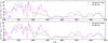 |
Fig. A.1. Comparison of the Fe II spectrum from our source with the best χ2 solutions employing the first three ratios (Section 3.3) in the computation. Top: Fe II spectrum assuming equal contribution from bright and dark sides, displayed with a 24% covering factor. The Fe II template corresponds to the CLOUDY simulation with logΦ(H) = 19.25 cm−2 s−1, log(Ptot) = 14 cm−3 K, Z = 20Z⊙ and Vturb = 40 km s−1. Bottom: Fe II spectrum assuming a 20% contribution from bright sides and 80% contribution from dark sides, displayed with a 33% covering factor. The Fe II template corresponds to the CLOUDY simulation associated with logΦ(H) = 19.75 cm−2 s−1, log(Ptot) = 15.50 cm−3 K, Z = 20Z⊙ and Vturb = 100 km s−1. |
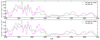 |
Fig. A.2. Same as in Figure A.1., but for the best χ2 solutions obtained by also employing the ratios discussed in Section 4.6. Top: Fe II spectrum assuming equal contribution from bright and dark sides, displayed with a 22% covering factor. The Fe II template corresponds to the CLOUDY simulation associated with logΦ(H) = 19.50 cm−2 s−1, log(Ptot) = 15.50 cm−3 K, Z = 20Z⊙ and Vturb = 40 km s−1. Bottom: Fe II spectrum assuming a 20% contribution from bright sides and 80% from dark sides, displayed with a 32% covering factor. The Fe II template corresponds to the CLOUDY simulation associated with logΦ(H) = 20 cm−2 s−1, log(Ptot) = 16 cm−3 K, Z = 20Z⊙ and Vturb = 100 km s−1. |
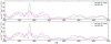 |
Fig. A.3. Same as in Figure A.1., but for the best χ2 solutions obtained using simulations that include mechanical heating as discussed in Section 4.5. Top: Fe II spectrum assuming equal contribution from bright and dark sides, displayed with a 4% covering factor. The Fe II template corresponds to the CLOUDY simulation associated with logΦ(H) = 18 cm−2 s−1, log(Ptot) = 14.75 cm−3 K, Z=Z⊙ and Vturb = 100 km s−1. Bottom: Fe II spectrum assuming a 20% contribution from bright sides and 80% from dark sides, displayed with an 8% covering factor. The Fe II template corresponds to the CLOUDY simulation associated with logΦ(H) = 18.25 cm−2 s−1, log(Ptot) = 14.75 cm−3 K, Z=Z⊙ and Vturb = 100 km s−1. |
Appendix B: Additional plots
We present here additional plots displaying an exemplary model with the addition of mechanical heating (Figure B.1.), and the best-fitting template for our Fe II model (Figure B.2.), and the structure and spectra of exemplary clouds simulated with CLOUDY in different conditions of constant density and constant pressure (Figure B.3.).
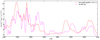 |
Fig. B.1. Comparison of the observed Fe II emission from the source with the Fe II model produced from a CLOUDY simulation including mechanical heating (also shown as the red line in Figure 2), assuming 25% covering factor after being convolved with a Gaussian kernel of FWHM = 2500 km s−1. |
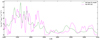 |
Fig. B.2. Fe II spectrum assuming a 20% contribution from bright sides and 80% contribution from dark sides with minimum χ2 employing the ratios in Sections 3.3 and 4.6, displayed with 33% covering factor after being convolved with a Gaussian kernel with FWHM = 2500 km s−1. The Fe II template corresponds to the CLOUDY simulation associated with logΦ(H) = 20 cm−2 s−1, log(Ptot) = 16 cm−3 K, Z = 20Z⊙ and Vturb = 100 km s−1. |
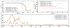 |
Fig. B.3. Structure and spectra of exemplary clouds simulated with CLOUDY at constant density (green and black), and constant pressure (red and orange), with different values of Vturb, assuming similar physical parameters. The ionizing flux was assumed logΦ(H) = 20 cm−2 s−1 for all clouds, and metallicity is assumed solar. Clouds in conditions of constant density have density fixed at log nH = 11 cm−3, while in case of constant pressure log(Ptot) = 16 cm−3 K. Top left: Cloud temperature profile in logarithmic scale as a function of depth (z) of the cloud. Top right: Cloud density profile in logarithmic scale as a function of depth (z) of the cloud. Bottom: Spectra of Fe II emission from different models, displayed with 100% covering factor. Each synthetic spectrum is broadened with a Gaussian kernel with FWHM = 2500 km s−1. |
All Tables
All Figures
|
Fig. 1. Top: Observed spectrum of RM 102, superimposed with the SDSS composite spectrum from Vanden Berk et al. (2001). The grey shaded regions define the spectral ranges from which the Fe II emission is extracted for the red-to-blue wings ratios in the UV and optical ranges (See Sect. 3.3). The SDSS composite is normalized at λ2800 Å. Bottom left: Zoomed-in on the UV Fe II emission, outlining the different spectral components adopted during fitting. Different Fe II templates (See Table 2 for reference) are displayed in different colours. Bottom right: Zoomed-in on the optical Fe II emission, outlining the different spectral components adopted during fitting, with the various Fe II templates (See Table 2 for reference) highlighted in different colours. |
| In the text | |
|
Fig. 2. Structure and spectra of exemplary clouds simulated with CLOUDY at constant pressure, assuming log(Ptot) = 16 cm−3 K, Vturb = 100 km s−1, Nc = 1024 cm−2 and Z = 10 Z⊙. The assumed values of ionizing fluxes are logΦ(H) = 18 cm−2 s−1 (displayed in green), 20 cm−2 s−1 (black) and 21 cm−2 s−1 (blue). An additional example with logΦ(H) = 18 cm−2 s−1 and the addition of extra mechanical heating is displayed in red. Top left: Cloud temperature profile in logarithmic scale as a function of depth (z) of the cloud. Top right: Cloud density profile in logarithmic scale as a function of depth (z) of the cloud. Bottom: Spectra of Fe II emission from different models, displayed with 100% covering factor. Each synthetic spectrum is broadened with a Gaussian kernel with FWHM = 2500 km s−1. |
| In the text | |
|
Fig. 3. Contour plots for the Ropt ratio described in Sect. 3.3 with constant Vturb = 0 km s−1, Z=Z⊙, and equal contributions from the bright sides and the dark sides of clouds. The position in the parameter space corresponding to the ratio measured in RM 102 is marked by a solid red line, while the dashed red line represents the 1-σ confidence range of the ratio. |
| In the text | |
|
Fig. 4. Contour plots denoting the ratios observed in the source RM 102 for different values of metallicity and microturbulence. The black, red, and blue contours denote RUV−opt, RUV, and Ropt, respectively. An orange dot in each plot marks the position of the best χ2 for each bin of metallicity. |
| In the text | |
|
Fig. 5. Contour plots denoting the ratios observed in the source RM 102 for different values of metallicity and microturbulence, assuming 20% contribution from the bright side of the cloud and 80% from the dark side. The RUV−opt contours are shown in black, the RUV contours are shown in red, and the Ropt contours are shown in blue. The position associated with the best χ2 for each bin of metallicity is marked with an orange dot. |
| In the text | |
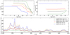 |
Fig. 6. Same as Fig. B.3., but for the best-fitting configurations described in Table 4. |
| In the text | |
|
Fig. 7. Top: Spectra of the Fe II emission obtained for several simulations in the Z = 20 Z⊙ and Vturb = 100 km s−1 grid. Grey-shaded regions indicate spectral ranges used to compute RUV and Ropt. Each template is normalized by the f parameter to match the integrated flux of the RM 102 spectrum in the 2000–5500 Å range. The figure demonstrates that no simulation accurately reproduces the observed Fe II emission across all grey-marked regions. Synthetic spectra are broadened using a Gaussian kernel with FWHM = 2500 km s−1. Bottom: Same as the top figure, but for 20% contribution from the bright side and 80% from the dark side. |
| In the text | |
|
Fig. A.1. Comparison of the Fe II spectrum from our source with the best χ2 solutions employing the first three ratios (Section 3.3) in the computation. Top: Fe II spectrum assuming equal contribution from bright and dark sides, displayed with a 24% covering factor. The Fe II template corresponds to the CLOUDY simulation with logΦ(H) = 19.25 cm−2 s−1, log(Ptot) = 14 cm−3 K, Z = 20Z⊙ and Vturb = 40 km s−1. Bottom: Fe II spectrum assuming a 20% contribution from bright sides and 80% contribution from dark sides, displayed with a 33% covering factor. The Fe II template corresponds to the CLOUDY simulation associated with logΦ(H) = 19.75 cm−2 s−1, log(Ptot) = 15.50 cm−3 K, Z = 20Z⊙ and Vturb = 100 km s−1. |
| In the text | |
|
Fig. A.2. Same as in Figure A.1., but for the best χ2 solutions obtained by also employing the ratios discussed in Section 4.6. Top: Fe II spectrum assuming equal contribution from bright and dark sides, displayed with a 22% covering factor. The Fe II template corresponds to the CLOUDY simulation associated with logΦ(H) = 19.50 cm−2 s−1, log(Ptot) = 15.50 cm−3 K, Z = 20Z⊙ and Vturb = 40 km s−1. Bottom: Fe II spectrum assuming a 20% contribution from bright sides and 80% from dark sides, displayed with a 32% covering factor. The Fe II template corresponds to the CLOUDY simulation associated with logΦ(H) = 20 cm−2 s−1, log(Ptot) = 16 cm−3 K, Z = 20Z⊙ and Vturb = 100 km s−1. |
| In the text | |
|
Fig. A.3. Same as in Figure A.1., but for the best χ2 solutions obtained using simulations that include mechanical heating as discussed in Section 4.5. Top: Fe II spectrum assuming equal contribution from bright and dark sides, displayed with a 4% covering factor. The Fe II template corresponds to the CLOUDY simulation associated with logΦ(H) = 18 cm−2 s−1, log(Ptot) = 14.75 cm−3 K, Z=Z⊙ and Vturb = 100 km s−1. Bottom: Fe II spectrum assuming a 20% contribution from bright sides and 80% from dark sides, displayed with an 8% covering factor. The Fe II template corresponds to the CLOUDY simulation associated with logΦ(H) = 18.25 cm−2 s−1, log(Ptot) = 14.75 cm−3 K, Z=Z⊙ and Vturb = 100 km s−1. |
| In the text | |
|
Fig. B.1. Comparison of the observed Fe II emission from the source with the Fe II model produced from a CLOUDY simulation including mechanical heating (also shown as the red line in Figure 2), assuming 25% covering factor after being convolved with a Gaussian kernel of FWHM = 2500 km s−1. |
| In the text | |
|
Fig. B.2. Fe II spectrum assuming a 20% contribution from bright sides and 80% contribution from dark sides with minimum χ2 employing the ratios in Sections 3.3 and 4.6, displayed with 33% covering factor after being convolved with a Gaussian kernel with FWHM = 2500 km s−1. The Fe II template corresponds to the CLOUDY simulation associated with logΦ(H) = 20 cm−2 s−1, log(Ptot) = 16 cm−3 K, Z = 20Z⊙ and Vturb = 100 km s−1. |
| In the text | |
|
Fig. B.3. Structure and spectra of exemplary clouds simulated with CLOUDY at constant density (green and black), and constant pressure (red and orange), with different values of Vturb, assuming similar physical parameters. The ionizing flux was assumed logΦ(H) = 20 cm−2 s−1 for all clouds, and metallicity is assumed solar. Clouds in conditions of constant density have density fixed at log nH = 11 cm−3, while in case of constant pressure log(Ptot) = 16 cm−3 K. Top left: Cloud temperature profile in logarithmic scale as a function of depth (z) of the cloud. Top right: Cloud density profile in logarithmic scale as a function of depth (z) of the cloud. Bottom: Spectra of Fe II emission from different models, displayed with 100% covering factor. Each synthetic spectrum is broadened with a Gaussian kernel with FWHM = 2500 km s−1. |
| In the text | |
Current usage metrics show cumulative count of Article Views (full-text article views including HTML views, PDF and ePub downloads, according to the available data) and Abstracts Views on Vision4Press platform.
Data correspond to usage on the plateform after 2015. The current usage metrics is available 48-96 hours after online publication and is updated daily on week days.
Initial download of the metrics may take a while.