| Issue |
A&A
Volume 689, September 2024
|
|
|---|---|---|
| Article Number | A321 | |
| Number of page(s) | 31 | |
| Section | Extragalactic astronomy | |
| DOI | https://doi.org/10.1051/0004-6361/202450458 | |
| Published online | 23 September 2024 | |
Chemical abundances along the quasar main sequence
1
National Institute for Astrophysics (INAF), Astronomical Observatory of Padova, 35122 Padova, Italy
2
Dipartimento di Fisica e Astronomia, Università di Padova, Vicolo dell’ Osservatorio 3, 35122 Padova, Italy
3
Laboratório Nacional de Astrofísica, MCTI, R. dos Estados Unidos 154, Nações, 37504-364 Itajubá, Brazil
4
School of Physics and Astronomy, Tel Aviv University, Tel Aviv, 69978, Israel
5
Instituto de Astrofísica de Andalucía (IAA-CSIC), Glorieta de Astronomía s/n, 38038 Granada, Spain
6
Center for Theoretical Physics, Polish Academy of Sciences, Al. Lotników 32/46, 02-668 Warsaw, Poland
Received:
20
April
2024
Accepted:
27
May
2024
Context. The main sequence of quasars has emerged as a powerful tool for organizing the observational and physical characteristics of type-1 active galactic nuclei (AGNs).
Aims. In this study, we present a comprehensive analysis of the metallicity of the gas in the broad-line region, incorporating both new data and previously published findings, to assess the presence of any trend along the main sequence.
Methods. We performed a multicomponent analysis on the strongest ultraviolet (UV) and optical emission lines for a sample of 13 radio quiet quasars in the 0.009 ≤ z ≤ 0.472 redshift range, selected based on the availability of multiwavelength data. We employed UV and optical data obtained from the Hubble Space Telescope (mainly from the Cosmic Origins Spectrograph and Faint Object Spectrograph) and several ground-based observatories, respectively. We then measured ten diagnostic ratios and compared them with the prediction of CLOUDY photoionization simulations, identifying the closest photoionization solution to the data.
Results. Our investigation reveals a consistent pattern along the main sequence. We observe a systematic progression in metallicity, ranging from subsolar values to metallicity levels several times higher than solar values.
Conclusions. These findings underscore the fundamental role of metallicity in correlating with the main sequence of quasars. Extreme metallicity values, at least several dozen times the solar metallicity, are confirmed in low-z AGNs radiating at a high Eddington ratio, although the origin of the extreme enrichment remains open to debate.
Key words: methods: observational / galaxies: active / quasars: emission lines / quasars: general / quasars: supermassive black holes / galaxies: Seyfert
© The Authors 2024
 Open Access article, published by EDP Sciences, under the terms of the Creative Commons Attribution License (https://creativecommons.org/licenses/by/4.0), which permits unrestricted use, distribution, and reproduction in any medium, provided the original work is properly cited.
This article is published in open access under the Subscribe to Open model. Subscribe to A&A to support open access publication.
1. Introduction
In recent years, the main sequence (MS) of quasars (Sulentic et al. 2000b; Marziani et al. 2001, 2010; Shen & Ho 2014) has proved to be a crucial tool for unraveling the spectral properties of type 1 active galactic nuclei (AGNs, e.g., Panda et al. 2019b; Panda & Śniegowska 2024; Fu et al. 2022; Wang et al. 2022; Nagoshi & Iwamuro 2022, among the most recent works), even at the highest redshifts (e.g., Yang et al. 2023; Loiacono et al. 2024). The MS is the parameter space defined by RFeII (the ratio between the intensity of the FeII emission at λ4570 to Hβ) and the Full Width at Half Maximum of Hβ: FWHM(Hβ) (Gaskell 1985; Boroson & Green 1992). The MS allows for the definition of two main populations of quasars occupying different regions of this parameter space (Sulentic et al. 2000a, 2011; Marziani et al. 2018b; Panda et al. 2024):
-
Population A (Pop. A), found below 4000 km s−1 of FWHM(Hβ), and
-
Population B (Pop. B), found above 4000 km s−1 of FWHM(Hβ).
A subpopulation of Pop. A AGNs, characterized by RFeII ≳ 1, is the extreme Pop. A (xA), which is associated with extreme-accreting AGNs (Marziani & Sulentic 2014; Du et al. 2016; Panda & Marziani 2023). These populations exhibit different spectral features associated with an array of physical conditions in the broad-line region (BLR) of these objects (Fraix-Burnet et al. 2017; Marziani et al. 2018b; Panda et al. 2019b).
Several parameters vary along the MS (see e.g., Sulentic et al. 2011; Fraix-Burnet et al. 2017; Panda 2021a, for summaries). Trends involve parameters associated with line formation, such as the ionization parameter, U, which has been shown to gradually increase moving from xA to Pop. B objects (Sulentic et al. 2000b; Marziani et al. 2010). The gas density, nH, seems to follow an inverse trend to U, with xA objects associated with much higher densities than Pop. B objects (Marziani et al. 2001; Matsuoka et al. 2008; Negrete et al. 2012; Martínez-Aldama et al. 2015; Panda et al. 2018). Notably, RFeII is believed to be primarily driven by the Eddington ratio, L/LEdd (Boroson & Green 1992; Marziani et al. 2001; Sun & Shen 2015; D’Onofrio et al. 2021). The position of objects along the MS is thus connected to the radiation emitted by the AGN continuum source, which is itself connected to the rate of accretion of matter onto the supermassive black hole (SMBH).
The FWHM(Hβ) is strongly affected by the viewing angle, even if the objects considered in the MS are all type 1 AGNs. There is increasing evidence that the low-ionization lines (LILs) are emitted in a flattened configuration corresponding to the accretion disk (e.g., Decarli et al. 2011; Mejía-Restrepo et al. 2018; Negrete et al. 2018; Panda 2021b), as was suggested a long time ago (Collin-Souffrin et al. 1988). The effect of the viewing angle on the line width (roughly proportional to sin θ, where θ is the angle between the line of sight and the accretion disk axis) is compounded by the effect of the SMBH mass that is weak but that becomes significant if AGNs in luminosity ranges of several orders of magnitudes are considered (Marziani et al. 2018a). If no correction for the viewing angle is applied, the Pop. B objects, by definition with larger FWHM, are characterized by systematically more massive SMBHs than their Pop. A counterparts (Marziani et al. 2003b).
The role of the chemical content of the BLR is, however, not yet completely understood in the process of line formation. Previous studies like those of Śniegowska et al. (2021) and Garnica et al. (2022) have focused on the metal content of xA quasars and determined high metallicity, Z, in the BLR of these objects, reaching extreme values. High Z is a potential explanation for the observed trends of density and ionization parameter, as resonant scattering becomes more efficient when metals are more abundant (e.g., Murray et al. 1995). Additionally, various studies have indicated the systematic enrichment of the BLR of AGNs compared to their host galaxies, nearly always reaching super-solar values (e.g., Hamann & Ferland 1999; Nagao et al. 2006; Xu et al. 2018; Maiolino & Mannucci 2019, and references therein). High Z values have been confirmed through independent techniques, such as iron emission and absorption features detected in the nuclear region (Jiang et al. 2018; Maiolino & Mannucci 2019). Some proposed explanations include selective enrichment of the circumnuclear region of the AGN (Śniegowska et al. 2021). Metallicities around the solar metallicity are possible for xA sources only under the most extreme conditions (Temple et al. 2021). In addition, there is still the possibility that the adopted empirical and photoionization models are inadequate.
Recent works suggest that enrichment may not occur for the BLR gas of all AGNs: toward the opposite extreme of the sequence, the estimation of metallicity indicates a solar metallicity (for the radio-quiet Pop. B) or a subsolar one (for the radio-loud Pop. B; Punsly et al. 2018; Marziani et al. 2022). Previous studies involved a few objects and samples in different redshift and luminosity domains (S21,G22,M23), focusing on specific spectral bins or populations of the MS. It is necessary to understand what happens between the extremes of the MS, and attempt to uncover any trend in metallicity along the MS that could unveil possible mechanisms behind the evolution of quasars and their host galaxies: evidence of blueshifts (Zamanov et al. 2002; Komossa et al. 2008; Boroson 2005; Aoki et al. 2005; Zhang et al. 2011; Negrete et al. 2018) in the lines of the spectra of most AGNs hints at the possibility that outflows could chemically enrich the gas found in the interstellar medium (ISM) or even the intergalactic medium (IGM) (Choi et al. 2024; Sabhlok et al. 2024). Indeed, Harrison et al. (2014) pointed out the far-reaching impact of such outflows beyond the BLR of these objects, suggesting an interplay between the enriched material produced in the regions close to the active nucleus and expelled over time in the direction of the host galaxy.
In this work, we present the systematic study of the metallicity of a sample of objects covering most spectral types along the MS at low redshift (Section 2). Section 3 describes the methodology and techniques used. Results for the objects of the sample are provided in Section 4. In Section 5, we address the potential issues of our methodology. The discussion of the results in Section 6 focuses on the correlation of the metallicity of objects with accretion parameters and the possible enrichment mechanisms that may explain our results. The conclusions are summarized in Section 7.
2. Sample
The sample of objects used in this work was selected based on a few criteria:
-
The availability of ground observations in the optical wavelength range of objects below a redshift z of 0.8, where Hβ can be observed.
-
The availability of archival ultraviolet (UV) data from HST covering the λ1300–2100 Å rest-frame range of the object.
-
The requirements of radio quiet (RQ) objects, to study the properties of the BLR without the influence of a collimated jet (Baker et al. 1994; Punsly et al. 2018; Gaur et al. 2019).
Table 1 reports the main observational parameters, in the following order: common name, IAU coordinate name, adopted redshift, Hβ FWHM, the FeII-to-Hβ intensity ratio, RFeII (with FeII emission integrated over the λ4434 − 4684 Å range, and Hβ measured on the full broad profile), the spectral type (ST) based on Hβ FWHM and RFeII, and Kellerman’s ratio (Kellermann et al. 1989), which is necessary to distinguish RQ objects from RL ones, defined as

Basic sample properties.
using data from the NED database. Here, fRadio is the specific flux at a wavelength of λ = 6 cm (5 GHz) and fB is the specific flux at λ = 4400 Å (680 THz) in the B band. When the NED data was not available, the specific flux used in the calculation was obtained from other works. The last two columns summarize the UV and optical data sources for each object.
Most objects that satisfied these selection criteria were included in the sample of objects in Marziani et al. (2003a). The spectra of PHL 1092, which is the most extreme object in the sample, were obtained from Marinello et al. (2020).
Figure 1 describes the distribution of the objects of the sample in bolometric luminosity (and computed in Section 6.2) and z, confronting them with average values from the samples used in the works of Śniegowska et al. (2021), Garnica et al. (2022), and Marziani et al. (2023) (hereafter referred to as S21, G22, and M23, respectively).
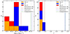 |
Fig. 1. Stacked histograms depicting the distribution of sample objects in log(Lbol) and z, categorized by the respective population. Assigned colors correspond to the legend, while vertical lines denote average values from the objects used in the referenced works S21, G22, and M23. |
3. Methodology
3.1. Subdivision of spectral types
An advantage of the MS is the possibility of defining spectral types along the optical plane of the sequence with simple selection criteria (Sulentic et al. 2002; Shen & Ho 2014; Panda & Śniegowska 2024). The expectation is that the effect of systematic trends along the sequence is minimized in each spectral type, so that an average spectrum of the sources in each bin is representative of all or most of the individual sources, not only phenomenologically, but also in terms of physical properties. This has been shown to be the case (Sulentic et al. 2002; Bachev et al. 2004; Marziani et al. 2010), even with some limitations (Marziani et al. 2001, 2018a,b; Panda et al. 2019b), as the 2D optical MS is not a simple 1D trend (Wildy et al. 2019; Martínez-Aldama et al. 2021), but rather the projection of a trend in a 4D space (the so-called 4DE1 space, Sulentic et al. 2000b).
In this paper, we follow the naming convention and the subdivision of Sulentic et al. (2002) in regular steps of δRFeII = 0.5 (increasing numerals with increasing RFeII), and δFWHM Hβ = 4000 km s−1 (A, B, and afterward B+, B++, etc.).
3.2. Emission line interpretation and empirical modeling
In this work, we adopt an interpretation of the emission line profiles of Type-I AGNs based on three main components:
-
Broad component (BC): A virialized component that constitutes the bulk of the line profiles of the main emission lines. It follows a Lorentzian profile in Pop. A objects and a Gaussian profile in Pop. B objects (Marziani et al. 2010). It is a distinctive component of Type-I AGN line profiles, identifying the BLR of these objects.
-
Blueshifted component (BLUE): A blueshifted outflow component present in the lines of almost all AGNs, affecting broad and narrow lines (Bachev et al. 2004; Zamanov et al. 2002). It is typically modeled by a skewed Gaussian that exhibits an asymmetry toward the blue (Zhang et al. 2011). This component is predominant in xA objects that are characterized by strong winds, and is mainly present in high ionization lines (HILs) like CIV.
-
Very broad component (VBC): A virialized component with a larger FWHM than the BC, as it models regions of the BLR that are closer to the SMBH (a very broad-line region (VBLR), Peterson & Ferland 1986; Sulentic et al. 2000c; Snedden & Gaskell 2007). It is a component exclusive to Pop. B objects that are modeled with a Gaussian that is redshifted by several km s−1 to the rest-frame wavelength of the emission line. It is a simplification introduced to account for the gradients more properly modeled in the “locally optimally emitting clouds” (LOCs) scheme (Baldwin et al. 1995) that accounts for the stratification of properties in the BLR, assuming that there is a gradual gradient of variation in properties in the BLR that follows a power law.
An additional component that can be encountered is the narrow component (NC), which is, however, not associated with the BLR, and thus modeled with narrow lines and disregarded in the estimation of the metallicity of the gas in the BLR.
3.3. Multicomponent fitting technique
Our sample was analyzed using the specfit (Kriss 1994) task from IRAF, inspecting the regions of our spectra centered on the SiIV+OIV]λ1400, CIVλ1549, C III]λ1909 (hereafter, SiIV+OIV], CIV, C III], respectively), and Hβ lines. The laboratory vacuum wavelengths of these lines, as well as all other lines measured during the analysis, are from Vanden Berk et al. (2001). The specfit task runs on the Space Telescope Science Data Analysis System (STSDAS) contrib package of IRAF, which was developed by the National Optical Astronomy Observatory (NOAO) in Tucson, Arizona (Tody 1986, 1993).
Specfit allows users to interactively fit a wide range of emission and absorption lines on the continuum model of the input spectrum. To achieve this, it employs input ASCII files created using the dbcreate task, containing the necessary functions to model various components of the spectrum. Gaussian and Lorentzian functions, widely used in multicomponent fitting, are each described by the values of the line intensity, central wavelength, FWHM, and asymmetry parameter. In addition to the standard functions provided, specfit allows the use of user-provided functions. In particular, we utilized the usercont and userline functions to model the complex FeIII (found in the UV range) and FeII (also found in the optical range) emissions, respectively.
The specfit multicomponent fitting procedure is interactive, based on the input file described in the previous paragraphs. The initial parameter values in the input file serve as starting guesses for modeling the components. Each parameter can be refined using a minimization fit provided by the routine. When the algorithm converges successfully, it provides the best-fit parameters that minimize the χ2 between the model and the observed data, resulting in an optimal solution. This fitting is carried out with two different algorithms (out of the five available in specfit):
-
Marquardt is based on the Levenberg-Marquardt (LM) algorithm, which iteratively minimizes the χ2 using the Jacobian matrix. This matrix contains the partial derivatives of the model function fitting the data to each fit parameter. The algorithm combines gradient descent and Gauss-Newton methods, adjusting the step size at each iteration. It takes larger steps when the fitting improves and smaller steps when it does not.
-
The downhill Simplex algorithm utilizes an iterative method for fitting, and for adjusting values for user-provided components, starting from initial guesses and constraints. It iteratively improves the solution toward the minimum χ2 with operations on an N-dimensional (the number of free parameters) simplex (Press et al. 1992). Unlike the LM method, the simplex algorithm requires only function evaluations and no derivatives. Even if it is not efficient in terms of the iteration number, it is very robust and never causes the specfit task to crash.
We started by fitting the continuum emission in the wavelength range with a power law function, carefully selecting regions of the spectrum unaffected by the presence of emission or absorption lines. The flux values of the continuum at various reference wavelengths are provided in Table 2.
Flux and uncertainty measurements.
In the optical wavelength range, we incorporated a FeII template to correct for FeII contamination, which can act as a pseudo-continuum on the modeled spectrum and which is particularly problematic in objects with strong FeII emission. Our Fe II template was derived from a European Southern Observatory (ESO) spectrum of I Zw 1 (Marziani et al. 2009, 2010, 2021). To address FeIII contamination, which is prevalent in the λ1800–2100 Å wavelength range, we utilized a template from Vestergaard & Wilkes (2001) based on the FeIII emission of I Zw 1. In cases in which the FeIII emission is strong, and there is evidence of a stronger feature at 1914 Å to the template, we modeled the 1914 Å feature with a Gaussian profile, even if it was severely blended with CIII]. This step is typically necessary for xA objects.
When fitting emission lines, we allowed them to vary, while imposing a rule that the NC of lines remain fixed at the rest frame of the object. Additionally, we ensured that the FWHM of SiIV+OIV] was similar to those measured for CIV and Hβ (Marziani et al. 2010). This is because lines associated with the virialized component of Hβ, CIII], CIV, and SiIV+OIV] are produced in approximately the same regions. By the same token, BLUE and VBC widths and asymmetries are also made consistent in the fit.
All of the measurements reported in the tables throughout the paper and those employed in the metallicity computations have been corrected for galactic extinction for each object using the equations of Cardelli et al. (1989).
3.4. Estimation of uncertainties
The placement of the continuum is one of the main sources of uncertainty in measuring emission-line intensities. In particular, the continuum placement strongly influences extended features such as the FeIII and HeIIλ1640 emissions in the UV range, and the FeII emission in the Hβ range.
The uncertainty associated with continuum placement was estimated as follows (cf. Śniegowska et al. 2021): initially, the intensity of the continuum was measured using IRAF in each range in which the best fit was conducted, yielding the root mean square (RMS) of the flux (measured in units of 10−15 erg s−1 cm−2
 ), as is shown in Table 2. Subsequently, the intensity of each line was measured by fixing the continuum’s intensity at both maximum and minimum values, by adding or subtracting the RMS, to obtain the line’s intensity at its minimum and maximum, respectively. When the continuum is higher (lower), the line intensity decreases (increases), compensating for the flux change, resulting in lower (upper) limits that are asymmetric and represent the range of emission line intensities.
To handle these uncertainties, we have assumed that the error distribution follows a triangular distribution (D’Agostini 2003). This simplifies error computation and is the preferred method for dealing with asymmetric uncertainties. For each line measurement, the variance σ2(X) of any parameter X was calculated using the formula for the triangular distribution:
where Δx+ and Δx− represent the differences between measurements with the maximum and best continuum, and with the best and minimum continuum, respectively. Finally, errors in spectral diagnostic ratios were calculated using standard error propagation formulas.
3.5. CLOUDY photoionization simulations
To constrain the properties of the gas in the BLR, we conducted photoionization simulations using the CLOUDY spectral synthesis code (Ferland et al. 2017). CLOUDY is a C++ code that models the ionization, chemical, and thermal state of the material that may be exposed to an external radiation field or other sources of heating. It predicts observables, including emission and absorption spectra, by solving the statistical and thermal equilibrium equations for many chemical species, including ions. The code accounts for collisional excitations and radiative processes, and treats radiation transfer through an escape probability formalism.
Photoionization simulations require input parameters that define ionization and level populations, along with electron temperature and optical thickness as a function of the geometrical depth within the emitting gas cloud. The assumed geometry is open and plane-parallel, representing a cloud of emitting gas as a slab exposed to a radiation field on only one side. The input parameters for a complete computation of the gas state, used to predict emission line intensities, include:
-
The ionization parameter, U, defined by the equation
where Q(H) is the number of ionizing photons and rBLR is the distance between the continuum source and the line emitting gas. It provides the ratio between the hydrogen-ionizing photons and the hydrogen number density.
-
Hydrogen gas number density, nH [cm−3].
-
Metallicity, Z, to solar metallicity, Z⊙, defined as
![$ \log Z = \log\left[\frac{Z}{H}\right] - \log\left[\frac{Z}{H}\right]_\odot $](/articles/aa/full_html/2024/09/aa50458-24/aa50458-24-eq7.gif) , where
, where ![$ \left[\frac{Z}{H}\right] $](/articles/aa/full_html/2024/09/aa50458-24/aa50458-24-eq8.gif) and
and ![$ \left[\frac{Z}{H}\right]_\odot $](/articles/aa/full_html/2024/09/aa50458-24/aa50458-24-eq9.gif) are the ratio of the measured number density of metals to hydrogen, and the same quantity for the Sun, respectively.
are the ratio of the measured number density of metals to hydrogen, and the same quantity for the Sun, respectively. -
Spectral energy distribution (SED) of the quasar.
-
Column density, Nc.
-
Microturbulence parameter.
This resulting 6D parameter space is not typically fully explored, and in our case we examined trends using arrays of simulations that were organized as follows. We used three different SEDs, one for each of the following cases: Pop. B RQ (Laor et al. 1997a), an SED for Pop. A sources (Mathews & Ferland 1987), and one for xA quasars (Ferland et al. 2020). Z was assumed to scale as solar (Z⊙), with 12 values ranging between 0.01 and 1000 Z⊙ for Pop. A and xA sources, and 14 values between 0.001 and 20 Z⊙ for Pop. B. The microturbulence parameter was set to 0 km s−1. This is negligible for resonance UV lines, as is outlined in Śniegowska et al. (2021), but is expected to lead to an underprediction of FeII emission (Sigut & Pradhan 2003; Bruhweiler & Verner 2008; Panda et al. 2018, 2019a; Śniegowska et al. 2021; Panda 2021b). For each metallicity value, we considered an array of simulations covering the nH and U parameter plane in the range of 7 ≤ log nH ≤ 14 cm−3, −4.5 ≤ log U ≤ 1 for Pop. A (667 simulations) and 7 ≤ log nH ≤ 13 cm−3, −3 ≤ log U ≤ 1 for Pop. B (425 simulations).
The separation of the three components (BC, VBC, and BLUE) can be heuristically associated with three different regions expected to be in different physical conditions, BLR, VBLR, and BLUE (see also the scheme in Fig. 2 Deconto-Machado et al. 2023). A source of uncertainty comes from the fact that photoionization computations were carried out under the assumption of single-zone emission, albeit separately for each of the three regions. While this assumption seems a good one for the BLR of extreme Pop. A, in which density and ionization tend toward limiting values (Marziani et al. 2001; Panda et al. 2019b; Panda 2021b), this might not be the case for Pop. B sources (Korista & Goad 2000), or for the less-extreme part of Pop. A.
3.6. Diagnostic ratios
Diagnostic ratios of lines provide constraints on the ionization, metallicity, and density of the emitting gas in the BLR. The following diagnostic ratios were used for computing the metallicity of our low-z quasar sample.
-
(SiIV+OIV])/CIV: widely used as a metallicity indicator (Nagao et al. 2006; Shin et al. 2013). An explanation of why this ratio is a reliable metallicity indicator is provided by Huang et al. (2023). In short, the ionic fraction of Si+3 increases with metallicity (the continuum right above the ionization potential of Si+2 2.5 Ryd remains significant), while the ionic fraction of C+3, conversely, strongly decreases with metallicity, as the continuum above 4 Ryd is almost completely absorbed in the innermost layers of the emitting gas. Even if both lines are diminished because the electron temperature goes down as metal abundance goes up, the ratio of SiIV+OIV]/CIV increases because of the decreasing C+3 ionic fraction with metallicity.
-
(SiIV+OIV])/HeII: sensitive to metallicity, assuming that the He abundance relative to hydrogen is constant. The OIV] line has a critical density of nc∼ 1011 cm−3 (Marziani et al. 2020), making this diagnostic ratio affected by density.
-
CIV/HeII: diagnostic ratio sensitive to metallicity, again assuming a constant He abundance relative to hydrogen. The reasons why the SiIV+OIV]/HeIIλ1640 and CIV/HeIIλ1640 are very reliable metallicity indicators are similar. First, there is the linear increase in the abundance of Si and C to He with increasing Z. In the CIV/HeIIλ1640 case, the ionization potentials of C2+ and He+ are almost coincident; however, the main difference is that HeIIλ1640 is a recombination line and the CIV is due to collisional excitation (Marziani et al. 2020; Śniegowska et al. 2021). As the metallicity Z increases, the electron temperature, Te, decreases (e.g., Pagel et al. 1979), and hence metal line excitation is disfavored. Conversely, the lower Te increases the rate of He++ recombination, reinforcing the increase in the ratios with Z. The ratio CIV/HeIIλ1640 has been used (Shin et al. 2013; Sulentic et al. 2014) despite the HeIIλ1640 weakness. However, with high S/N and resolution measurements from the Faint Object Spectrograph (FOS), and especially the Cosmic Origins Spectrograph (COS), we can accurately estimate the line intensity of HeIIλ1640, which was previously very difficult to assess, and self-consistently deblend it from the much stronger CIV emission.
-
CIV/Hβ: unlike all of the other ratios employed in this work, the CIV/Hβ ratio is subject to major observational uncertainty in the photometric precision of the optical data, and a lack of concurrent optical and UV observations. The depth of absorption features close to the rest frame in the CIV profile is difficult to assess and may significantly lower the CIV/Hβ (one of the most serious cases could be PHL 1092, Table 10). The diagnostic value of the CIV/Hβ ratio is primarily due to its strong dependence on the ionization parameter. Fig. 2 shows the behavior of the CIV/Hβ intensity ratio in the plane log Z, log U: the isophotal contours are almost parallel to the Z axis. In the presence of a very low CIV/Hβ (∼1) ratio, the U must be very low, with log U ≲ −2.5. At higher ionization parameters of −1 ≲ log U ≲ 0, and moderate density, the CIV emission to the Balmer line is optimized at relatively low values of Z. At higher Z (≳10 Z⊙), for the same U, the electron temperature is significantly lowered, decreasing the collisional excitation rate, and therefore lowering the line emission. There are two implications relevant to this work: a very weak CIV requires very low U, with the lowest CIV prominence obtained for low Z (Fig. 2). Conversely, for log U between 1 and 0, where CIV is efficiently produced, CIV/Hβ ≳ 10 can be achieved for log Z ∼ −2, with a density log nH between 11 and 13.
-
AlIII/CIV: a diagnostic ratio sensitive to the ionization parameter. This is because it relates lines of elements with different ionization potentials. It is potentially useful to constrain the effect of feedback from supernovæ since AlIII is overproduced in the explosion of type Ibc supernovae to the CIV solar abundances (Chieffi & Limongi 2013). This diagnostic ratio may tend to bias the estimated Z toward higher values.
-
AlIII/SiIII]: a diagnostic ratio sensitive to density, since it involves an intercombination line with a well-defined critical density of nc ∼ 1011 cm−3 for SiIII] (Negrete et al. 2013). If the ratio AlIII/SiIII] is ≫1, the resulting density will be much greater than the critical density. Historically, diagnostic ratios employing AlIII have rarely been used, since the measurement of the intensity of AlIII was quite uncertain, but with high-quality COS and FOS spectra, we have been able to measure it accurately.
-
SiIII]/CIII]: a diagnostic ratio sensitive to density, similar to AlIII/SiIII] but around lower values, nc ∼ 1010 cm−3 for CIII] (Hamann et al. 2002). Like the ratio described above, if SiIII]/CIII] is ≫1, the resulting density will be much greater than the critical density of CIII] as well, and is a very powerful density estimator, constraining density very well. The inclusion of strong CIII] may, however, bias the (U, nH, Z) solution toward lower densities. This issue is analyzed in Section 5.
-
CIII]/CIV: a diagnostic ratio sensitive to the ionization parameter as it compares the intensity of different ionization degrees of the same atomic species. However, since CIII] is an intercombination line, it is also sensitive to density. For xA sources, the ratio CIII]/CIV is subject to higher uncertainties due to FeIII contamination, making it difficult to measure the intensity of CIII] accurately. However, since xA CIII] is weakest along the MS (Bachev et al. 2004; Aoki & Yoshida 1999), a fairly high-density solution is suggested anyway despite the uncertainties.
-
FeII/Hβ: a diagnostic ratio sensitive to metallicity, as it involves a metal and hydrogen. However, this diagnostic ratio is also sensitive to the density, ionization parameter, and column density of the line-emitting gas (Verner et al. 1999, 2004; Bruhweiler & Verner 2008; Panda et al. 2018, 2019b; Panda 2021b). High FeII/Hβ is only possible if conditions of low ionization, high density (nH ≳ 1011 cm−3), and a large column density (Nc ≳1023 cm−2) are satisfied (Panda et al. 2018, 2019b; Panda 2021b). The ratio FeII/Hβ is relatively easy to measure with good precision (∼0.1 at a 1σ confidence level). However, the mean escape probability formalism is known to perform poorly in the prediction of the emission line strength for gas irradiated by strong X-ray sources (e.g., Dumont et al. 2003, and references therein). In the case of this particular ratio, there is therefore considerable uncertainty associated with the photoionization computations.
-
HeIIopt/Hβ: a diagnostic ratio sensitive to the ionization parameter. Assuming the abundance of He relative to hydrogen is constant, it is the ratio between two species with very different ionization potentials: HeIIλ4686 requires ∼50 eV to be ionized, while hydrogen requires ∼10 eV. The HeIIλ4686/Hβ ratio is relatively insignificant in the Z estimates.
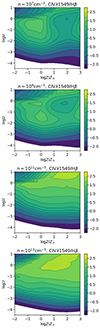 |
Fig. 2. Behavior of the diagnostic ratio, C IV/Hβ, (shown on a logarithmic scale) as a function of the ionization parameter, U, and metallicity, Z, for four values of hydrogen density, log nH = 7,9,11,13 [cm−3], using the Mathews & Ferland (1987) Pop. A SED. |
These diagnostic ratios are used differently depending on the quasar population. Notably, not all components are present in all objects. Although most objects can be modeled assuming a BLUE component for HILs, it is not always present for LILs. By the same token, the VBC appears only in Pop. B sources. For Pop. A objects, reliable estimation is only possible for physical parameters associated with the BC. For Pop. B quasars, it is possible to estimate the physical parameters of gas located in the VBLR and BLR, while for xA quasars it is possible to estimate the properties of the BLUE and BC. In this study, we exclusively examined the BLUE of PHL 1092, since it was the only object with a sufficient number of diagnostic ratios enabling an accurate constraint of its physical conditions.
The solution for the single-zone model, represented by a single point in the 3D space (nH, U, Z), was determined by minimizing the χ2 computed from the difference between the observed line ratios and the predicted line ratios across the entire 3D space (Marziani et al. 2024), applying the following relation:
with Rkc identifying the diagnostic ratio considered for the object and component, and δRkc identifying the error associated with each component. The “mod” subscript identifies the value of the specific diagnostic ratio predicted by the CLOUDY simulations for each value in the 3D grid of the (nH, U, Z) parameter space.
3.7. FeII and AlIII upper limits
CLOUDY photoionization simulations have previously hinted at the possibility of a contribution to the intensity of AlIII and FeII emission from the VBC for Pop. B Quasars and from the BLUE for xA Quasars (Zhou et al. 2023). This possibility was thus investigated by damping the intensity of AlIII emission obtained from the multicomponent fitting of our spectra, adding a Gaussian component to the fit with the same blueshift (redshift) for xA quasars (for Pop. B quasars) corresponding to the shift between the Hβ BC and the Hβ BLUE (Hβ VBC), and the same FWHM as the BLUE (VBC). After including this additional component, the χ2 associated with the fit was calculated for varying intensity values of the Gaussian line. As a result, regions associated with 1σ, 2σ, and 3σ compatibility were drawn in the plots shown in Figure 3. The same procedure was applied to the FeII emission in the optical wavelength range, with the difference that instead of adding a Gaussian component, the additional FeII emission was modeled from the ESO FeII template (Marziani et al. 2009, 2010). The results of this computation were then added to the known diagnostic ratios associated with the VBC or the BLUE of our objects, by using the 1σ upper limit as the diagnostic ratio.
 |
Fig. 3. Left: plot of the χ2/χmin2 distribution as a function of the relative intensity of the FeIIBC of PHL 1092 with respect to the specfit retrieved intensity, vs. the relative intensity of the FeIIBLUE with respect to the original intensity of FeIIBC. Middle: same, but for the AlIIIVBC emission of Fairall 9. Right: same, but for the FeIIVBC emission of Fairall 9. |
4. Results
4.1. Estimation of metallicity and physical parameters
Tables 3, 4, 5, and 6 report the intensity of each different line component for the objects of the sample measured from the multicomponent fitting, with associated errors, for the four spectral ranges that have been fit separately; namely, SiIV+OIV], CIV+HeIIλ1640, AlIII+Si III]+CIII], and Hβ+FeII. The fits are shown in the figures of Appendix A, and the projections of the (U, nH, Z) parameter space in Appendix B. Table 7 summarizes the diagnostic intensity ratios used for the estimation of the physical parameters. The estimates of the metallicity and physical conditions in the BLR for our sample were obtained using the methodology described in Section 3, and the results are reported in Table 8. Results for individual sources are discussed in more detail in Appendix C.
SiIV+OIV] blend line measurements.
CIV and HeIIλ1640 line measurements.
λ1900 blend line measurements.
Optical line measurements.
4.2. The trend along the main sequence
Figure 4 depicts the MS representation of our sample, alongside representative values from S21, G22, and M23. The main result is that the highest-metallicity objects are clustered in the xA region of the MS. Conversely, all other objects with solar or subsolar metallicities are situated in the left portion of the MS, demonstrating a gradient of metallicity that peaks in the xA segment of the MS and gradually decreases toward RL Pop. B sources – an outstanding result that confirms the theoretical predictions of Panda et al. (2019b). For the sources of ST A1 and B1 with stronger FeII, we encounter Z around solar, which becomes supersolar for RFeII ≳ 0.5. An important result is that these sources are at low z, and reach Z comparable to the samples of S21 and G22 that are high z and that are associated with quasars of very high MBH and extreme luminosity. Conversely, xA sources from the present sample are AGNs of moderate luminosity, narrow line Seyfert 1s (NLSy1s) with MBH ≲ 108 M⊙. Since the high-z objects are extreme radiators at a high Eddington ratio of Lbol/LEdd ∼ 1, as the xA of our sample are, the enrichment phenomenon appears to be independent of cosmic epoch and of black hole mass, at least up to cosmic ages of ∼3 Gyr after the Big Bang.
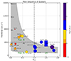 |
Fig. 4. MS representation of our sample. Every object is placed according to its RFeII and FWHM(Hβ). Greater metallicity, Z, is expressed with increasing marker sizes and different colors. Objects with subsolar metallicity are marked in red, objects with 1 Z⊙ ≤ Z ≤ 2 Z⊙ in orange, objects with 2 Z⊙ < Z ≤ 10 Z⊙ in gold, objects with 10 Z⊙ < Z ≤ 50 Z⊙ in blue, and objects with metallicity greater than 50 Z⊙ in indigo. Sources from this work are shown in circles. Squares are used as reference values for the objects in S21, G22, and M23, the latter with two squares, one for RL sources and the other for RQ sources. The gray region describes the typical positions occupied by objects along the MS (Zamfir et al. 2010; Garnica et al. 2022). |
The mechanisms that could explain the high-Z values and the presence of a gradient of metallicity are briefly discussed in Section 6.5.
5. Validation
In the following sections, we discuss the limits of our technique and the tests that we used to address these limits.
5.1. Statistical errors
The minimum χ2 criterion and the F-test are not suited to estimate the influence of statistical errors. In this respect, bootstrap repetition of the Z, nH, and U estimate allows for deviation from a perfect solution (i.e., from the diagnostic ratio values predicted by a definite model Z, nH, and U) and enables one to assess how large the relative uncertainties in the intensity ratios can be until the correct solution in terms of metallicity is lost. Bootstrap simulations were carried out, assuming random variations and following a Gaussian distribution with σ corresponding to several fractional uncertainties. In practice, each replication assigned new values to the ratios, following Gaussian deviates with a dispersion corresponding to the fractional uncertainty. Fig. 5 shows that the Z information is preserved for statistical errors up to ≈0.45 for the somewhat idealized case of ten diagnostic ratios having a constant fractional uncertainty, assuming diagnostic ratios from simulated cases with metallicity ranging from log Z = 0.3 to 1.7, which could be fairly typical for Pop. A and xA. The statistical uncertainties do not affect the Z estimates up to 0.3–0.35 fractional errors. Increasing the statistical uncertainties by 50% for ratios CIV/HeIIλ1640 and SiIV+OIV]/HeIIλ1640, because of the faintness of HeIIλ1640, lowers the highest uncertainty preserving the Z value by 0.05 (i.e., from 35% to 30%). The statistical errors tend to lower Z (as well as U and nH, which are not shown). Therefore, statistical fluctuations are unlikely to induce systematically higher values of the metallicity to the ones derived from the model and to account for the very high Z deduced for the extreme Pop. A sources. More relevant to the analysis of the result is the possibility of systematic discrepancies in emission line ratios to the expectation of a photoionization solution.
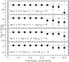 |
Fig. 5. Median Z values for 200 replications of the intensity ratios deviating from the ones predicted by four models as a function of fractional uncertainties. |
5.2. Alternative χ2 evaluations
The question is whether the technique employed for the χ2 estimate could be at the origin of the out-of-scale Z of PHL 1092, and of the very high values (Z ≲ 100) encountered among xA sources. The χ2 expression of Eq. (4) is weighting the contribution of each measurement on the inverse of the uncertainty squared. This is expected to be effective in increasing the likelihood of the solution, but at the same time gives minimum weight to “bad” data that have large uncertainty. Several ratios in Table 7 are between two detected lines, but have an uncertainty larger than the reported value. We therefore considered two alternatives to the χ2 technique reported in Table 8, and those are shown in Table 9.
Diagnostic intensity ratios.
Metallicity and physical parameter estimates along the quasar MS.
Different normalization for χ2 computation.
Instead of dividing each addendum by the error squared, the addenda could be divided by the value expected from the simulation for each (U, nH, Z) grid element (different for each U, nH, Z), or by the observed ratios that are constant. This last option especially offers a valid alternative to the conventional χ2 because it effectively quantifies the relative difference between any model and the observed set of ratios. Each ratio will have a weight independent from its associated uncertainty. If this exercise is carried out, the minimum χ2 solutions confirm the high Z values for both LB 2522 and PHL 1092. The Z derived for PHL 1092 BLUE even increases to 20–50 Z⊙. Therefore, the metallicity estimates at high Z do not appear strongly sensitive to the different choices of χ2 that we have considered.
5.3. Influence of optical-UV mismatch
Several sources are affected by an optical-UV flux mismatch, likely originated by observations conducted at different moments using both ground-based and space-based observatories. Optical observations are susceptible to uncontrollable light loss, significantly impacting the reliability of diagnostic ratios based on both optical and UV lines. However, diagnostic ratios dependent on lines found at similar wavelengths are less susceptible to this issue, as the intrinsic variability of the quasar should similarly affect them. The most likely candidate for this problem is the C IV/Hβ ratio, as it is the sole diagnostic ratio involving a UV line and an optical one.
Indeed, when estimating the physical parameters associated with the BLR of our sample of quasars, the CIV/Hβ ratio often disrupted the computation, returning combinations of U, Z, and nH that were not compatible with our previous assumptions, or solutions strongly incompatible with any of the CLOUDY simulations used in this work: very low C IV/Hβ values are possible for low U, for most Zs (Fig. 2). The values of CIV/Hβ along with the log U and log Z results obtained from the calculation are shown in Table 10. It is important to note that the CIV/Hβ ratio was excluded in most calculations (Table 7). The primary observation from Table 10 is that the CIV/Hβ value follows a clear pattern, steadily decreasing toward the most extreme xA sources. This pattern has been observed in other works and is a peculiar feature of xA quasars (Sulentic et al. 2017; Vietri et al. 2018), exhibiting the bulk of their CIV emission in the BLUE. However, despite being a physical result, inappropriate estimation of this ratio due to the aforementioned problems strongly affects the measurements of Z and U, rendering the estimation incorrect. The CIV/Hβ ratio, being particularly sensitive to U, loses its dependence on metallicity (represented in Figure 2), returning a solution that is not physical, distorting the results associated with other diagnostic ratios.
CIV/Hβ results.
5.4. Influence of the spectral energy distribution
The choice of the SED used for the photoionization simulations is expected to significantly influence the results obtained during the estimation of physical parameters in the BLR, as it dictates the luminosity of the central source. Population A and B sources typically display distinct spectral features, leading to remarkably different SEDs (see Figure 1 in Panda et al. 2019b). However, the distinction between Pop. A and xA sources is less clear-cut, particularly between the A2 and A3 spectral bins, as is observed in some objects in our sample that exhibit borderline features. Furthermore, the Pop. A SED has been used in other works (Marziani et al. 2024), since the xA SED employed in this work has often been considered too extreme for many Pop. A objects. To address this issue, we recalculated the χ2 using the Pop. A SED for xA sources, keeping track of the systematic changes encountered (as is summarized in Table 11). Additionally, in Figure 6, we illustrate the positions occupied by the results for both SEDs in the log U − log Z parameter space.
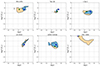 |
Fig. 6. Two-dimensional parameter space of log Z − log U illustrating the physical conditions of the gas surrounding xA sources with different SEDs. In each plot, the minimum χ2 computed between measured diagnostic ratios and CLOUDY simulations is shown with dots: green for the Mathews & Ferland (1987) SED and blue for the xA SED. The orange region corresponds to the 1σ accuracy range for the Mathews & Ferland (1987) SED, and the blue region for the xA SED. |
Metallicity and physical parameter estimates using Pop.A SED.
The primary outcome of this test was a systematic decrease in the minimum χ2 obtained for all xA objects, with the exception of PHL 1092 (which served as the basis for the xA SED). Furthermore, the solutions consistently indicate higher densities, typically moving upward by an order of magnitude or less. However, no significant changes to metallicity or U have been observed, as is depicted in Figure 6. Nonetheless, the parameter distributions obtained using the xA SED are generally more constrained.
5.5. Microturbulence and highest Z values
Microturbulence is believed to increase the efficiency of metal line production. This is especially true for FeII blends (Verner et al. 1999, 2004; Bruhweiler & Verner 2008; Panda et al. 2018), as microturbulence is expected to increase FeII self-fluorescence and fluorescent excitation due to continuum and strong emission lines. CLOUDY simulations were carried out starting from the (U, nH, Z) values of I Zw 1 and PHL 1092. The left panel of Fig. 7 shows the key intensity ratios CIV/HeIIλ1640, CIV/Hβ, and RFeII as a function of the microturbulent velocity. A microturbulent velocity of  km s−1 corresponds to the thermal broadening of lines emitted by gas at the electron temperature of the BLR, T ∼ 10 000 K. The effect of microturbulence passing from 0 to 10 km s−1 is a net increase in RFeII for PHL 1092, while the effect is less clear for I Zw 1. The right panel of Fig. 7 shows the trends for the same ratios, starting from low-ionization and high-density solutions, for three very high Z values; namely 50, 100, and 200 Z⊙. The effect on RFeII is remarkable in all three cases. The increase in the emission efficiency of FeII features implies that less iron is needed to produce the same line luminosity.
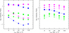 |
Fig. 7. Behavior of the diagnostic ratio CIV/He IIλ1640 (magenta), CIV/Hβ (blue), RFeII (green) on a logarithmic scale vs. microturbulence velocity in km s−1. Left: using the solution for I Zw 1 (squares) and PHL 1092 (circles). Right: Using a low-ionization, high-density solution appropriate for xA sources (see text for details), with three different Z values: 200 Z⊙ (circles), 100 Z⊙ (squares), and 50 Z⊙ (triangles). |
We recomputed the array of simulations for the Mathews & Ferland (1987) SED in the range of 7 ≤ log nH ≤ 14, −3.5 ≤ log U ≤ 0, and for ten values of Z between 1 and 1000 Z⊙. The results for PHL 1092 indicate a greatly reduced value of the metallicity,  [Z⊙]. The inclusion of turbulence aligns the estimate of the out-of-scale measurement to more likely values of Z ≲ 100 Z⊙. Most sources with Z ≥ 10 Z⊙ have their Z estimates unchanged or reduced by a factor of ≈2, as was first suggested in Panda (2021b). It is interesting to note that this reduction seems to occur only for the highest values of Z, while for lower metallicities around the solar metallicity, the effect of turbulence is not obvious.
5.6. Stratification
Evidence indicates trends for various parameters along the quasar MS. Specifically, in the case of Pop. B, there is observable evidence of a radial stratification of properties within the BLR (Baldwin et al. 1995; Korista et al. 1997). As was previously mentioned, this region was modeled by distinguishing between a BC and a VBC. However, it is not certain whether the assumption of constant physical parameters within the BLR is entirely accurate for Pop. A. On the one hand, the physical parameters appear to be associated with a much smaller uncertainty range in Pop. A than in Pop. B (compare Figures B.1, B.2, B.3 vs. B.4, B.5). On the other hand, several Pop. A sources show prominent CIII] that may bias the photoionization solution toward lower nH. To test whether the estimates of Z are stable to this potential bias, we repeated the Z estimates, removing the diagnostic ratios involving C III] for Mrk 335 and Ark 564, the objects that exhibit the lowest nH. The computation yielded different results for the two objects: Mrk 335 retained a very low density (log nH ≈ 7.5 [cm−3]), confirming the presence of low-density gas in its BLR, which is also supported by the fitting of a semi-BC of [O III]λλ4959,5007, as is described in Appendix C. Ark 564, on the other hand, returned a higher-density solution, with log nH ≈ 11 [cm−3], suggesting that the absorption feature affecting C III] led to an overestimation of its line intensity.
Figure 8 displays the trend of Z along the MS by analyzing the average value of Z across specific spectral types, averaging all the values obtained with the methods that most affect the determination. The trend in metallicity is evident from this figure, with a dip in metallicity for the A1 spectral type being influenced by the selection of objects in our sample. In the A1 spectral type, the average RFeII is lower than that measured for the adjacent bins: A1 sources are associated with lower RFeII than is typically measured in that spectral type, and thus contribute to lower estimations of Z. Additionally, the absence of CLOUDY simulations with log Z = −0.3, −0.7 for Pop. A objects contributed to an underestimation of Z. Nevertheless, the trend in metallicity proceeds quite steadily from Pop. B RL quasars to xA quasars.
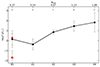 |
Fig. 8. Diagram illustrating the trend of Z across different spectral types, with the reference values for each spectral type obtained as the geometric mean of all the measurements assumed for all the objects belonging to a specific spectral type, including our method, the use of the CIV/Hβ ratio, and the presence of microturbulence for all sources belonging to the A2, A3, and A4 spectral types. Confidence intervals are obtained as the standard deviation of our results. The number of objects contributing to each spectral type is shown in green, along with the average RFeII of the sources considered. Two reference points (in red) are shown describing the RL and RQ Pop. B sources studied in M23. |
6. Discussion
6.1. A recipe to compute broad-line region metal content
Summarizing the procedure followed in this paper, we can define a recipe with several steps that could be easily applicable to larger samples of quasars:
-
Identification of the spectral type and radio loudness, or at least if an object belongs to Pop. B, Pop. A or extreme Pop. A. We note that RL xA AGNs are extremely rare in Pop. A at low z (Ganci et al. 2019);
-
Consideration of a maximum number of ratios for each component, avoiding ratios between two faint components;
-
Multicomponent fitting, to separate individual components associated with different associated physical conditions (Section 3.2);
-
Computation of the minimum χ2 between our measurements and the results obtained from CLOUDY photoionization simulations to cover the parameter space in terms of SED, Z, nH, U, and the microturbulence parameter. Ideally, SEDs should be different for at least Pop. B RQ and RL, Pop. A, and xA. The microturbulence parameter could be 0 or 10 km s−1;
-
Definition of 1σ confidence ranges via an F-test with an appropriate number of degrees of freedom.
In Section 5.3, we discussed that the presence of an optical-UV flux mismatch was a major obstacle encountered during this procedure. The effect of this mismatch, which plays a crucial role in nullifying the information of the CIV/Hβ diagnostic ratio, mostly affects objects with noncontemporary observations. However, the CIV/Hβ ratio is extremely effective at constraining U, so relinquishing this ratio has a negative impact on the accuracy of the measurement of the physical conditions in the BLR. We thus propose that the C IV/Hβ ratio should be used with the highest confidence in the case of contemporary observations in the UV and optical range. In this case, the diagnostic ratio has a positive effect on the measurement and should help retrieve well-constrained results.
The FeII/Hβ ratio has often yielded discrepant information with respect to CIV/Hβ. Indeed, this ratio is not typically predicted to be very high for the SEDs employed in this work. This raises the possibility that the optical ratios could be problematic for the estimation of the physical parameters, and should thus be excluded from the computation.
6.2. Estimation of accretion parameters
The bolometric luminosity (Lbol) of the AGNs of the sample was estimated using the relation
 d^2_{\rm P} = L(5100\,\AA ) k_{\rm bol}, \end{aligned} $$](/articles/aa/full_html/2024/09/aa50458-24/aa50458-24-eq33.gif)
where dP is the luminosity distance divided by (1+z). In this paper, the values of the cosmological parameters are adopted as follows: H0 = 70 km s−1 Mpc−1, ΩM = 0.3, and ΩΛ = 0.7. The bolometric correction factor kbol was calculated using the formula from Netzer (2019):
where L(5100 Å) is the luminosity of the quasar at 5100 Å. The mass of the black hole (MBH) was estimated using the relation
with I44 = L(5100 Å)/1044 erg s−1 obtained from Du & Wang (2019). The formula in Equation (7) is the Vestergaard & Peterson (2006) relation with two changes: (1) a correction on the FWHM following Mejía-Restrepo et al. (2018), and (2) the inclusion of the dependence of the BLR radius on RFeII (Du & Wang 2019). In practice, Eq. (7) rectifies the mass estimations for extreme accretors, while keeping the results unchanged for other objects.
The Eddington ratio was estimated using the formula Lbol/LEdd, with the Eddington luminosity, LEdd, obtained as follows:
The derived properties of the sample are shown in Table 12.
Derived properties of the sample.
6.3. Correlation with accretion parameters
We investigated the correlation of accretion parameters with metallicity and the RFeII parameter that defines the MS. Utilizing the SLOPESFORTRAN code outlined in Feigelson & Babu (1992), we calculated the Pearson’s correlation coefficient, rP, between the quantities. Subsequently, we determined the probability, P, of a spurious correlation, computed using the complementary error function, erfc , where x is defined as
  , with N representing the number of objects (Press et al. 1986).
The correlation analysis (Figure 9) yielded interesting results. The parameters correlating more strongly are RFeII and log(L/LEdd), with rP = 0.925. This result reinforces the hypothesis that the Eddington ratio is the physical parameter behind the RFeII, serving as the primary driver of the MS, as has been found by several works (Marziani et al. 2001; Sun & Shen 2015; Du et al. 2016; Panda et al. 2019b; Panda & Marziani 2023, see also the synopsis in D’Onofrio et al. 2021). Additionally, very robust correlations were also observed in this sample between RFeII and log Z, and between log(L/LEdd) and log Z, confirming once again that extreme-accreting sources are characterized by high metallicities (Martínez-Aldama et al. 2018; Śniegowska et al. 2021; Garnica et al. 2022). Moreover, the correlation in this work is extended to most spectral types along the MS, also including Pop. B sources, rather than being limited exclusively to xA sources as in Śniegowska et al. (2021) and Garnica et al. (2022). The presence of such strong correlations is not trivial, as these quantities were derived independently and using different procedures.
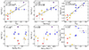 |
Fig. 9. Figures showing a correlation between various accretion parameters with log Z and RFeII. Points are displayed using the same color-coding as in Figure 4, with their error bars. When the correlation is considered significant (rP ≳ 0.7, corresponding to a confidence level of ≈0.01), the correlation line is shown, with its defining parameters intercept (A) and slope (B) shown with their respective errors. For each correlation are also shown the Pearson correlation coefficient, rP, from the SLOPES program (Feigelson & Babu 1992) and the probability, P, of a spurious correlation. |
Our results confirm the earlier finding concerning low-z PG quasars that the BLR gas Z correlates with Eddington ratio, while Z shows a much weaker correlation with MBH (Shin et al. 2013). Typical values of SiIV+OIV]/CIV and NV/CIV at low redshifts suggested values around the solar one or a few times higher than it. The range covered by the two diagnostic ratios was found to be consistent with those measured for a sample of intermediate-redshift quasars of a luminosity comparable to the one of luminous AGNs at low z (Sulentic et al. 2014). The trend with Lbol/LEdd is due to the inclusion of Pop. B, and spectral type A1s that are radiating at a lower Eddington ratio with respect to xA sources. The absence of a clear trend at intermediate z corresponding to the cosmic noon with a maximum of nuclear activity and star formation (e.g., Madau & Dickinson 2014; Florez et al. 2020; Förster Schreiber & Wuyts 2020), and the large Z estimated for quasars at that cosmic epoch, might just be the result of a selection effect disfavoring the lowest Lbol/LEdd for any given MBH (Sulentic et al. 2014).
The three remaining correlations depicted in Figure 9 were not found to be statistically significant. The absence of a significant correlation between log Z and log MBH was particularly puzzling, as these quantities have been found to correlate in other works (Xu et al. 2018; Maiolino & Mannucci 2019), and larger SMBHs were found to be the ones with the highest metallicity, since their stronger gravitational potential is able to trap the more metallic matter in their virialized region.
6.4. Comparison between the photoionization and reverberation solutions for rBLR
The computation of physical parameters in the BLR, coupled with Equation (3) for the ionization parameter, yields an independent measurement of rBLR, which could be compared with the results obtained from Hβ reverberation mapping for our sources (cf. Wandel 2000; Negrete et al. 2013). The reverberation, rBLR, or time delays are reported whenever available in the presentation of the individual objects of the sample (Appendix C). The rBLR estimations are compared in Figure 10. The two independent estimations yield similar results for most sources of our sample, within a factor of ∼3 (Vestergaard & Peterson 2006; Negrete et al. 2013; Panda 2022).
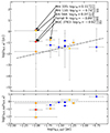 |
Fig. 10. Top: scatter plot showing the comparison of rBLR estimated with reverberation mapping (rBLR, RM), and using CLOUDY photoionization simulations (rBLR, Φ), on a logarithmic plane. Points are displayed using the same color-coding as in Figure 4, with their respective error bars. The dash-dotted line describes the position of objects for which the two independent determinations coincide. The values of rBLR, Φ for objects whose determinations do not coincide with rBLR, RM by a margin are shown in the upper right quadrant of the figure (expressed in pc), connected to their representative points through an arrow. An alternative result of the determination of physical parameters is shown for Ark 564 with a square, obtained by removing the diagnostic ratios employing CIII]. Bottom: plot showing the difference between the two estimations. The horizontal dash-dotted line describes the position of objects for which the two independent determinations coincide. The dotted line connects the two different determinations for Ark 564 described above. |
Three estimations of the BLR radius using the physical parameters obtained from our spectral measurements yield results incompatible with the reverberation mapping estimation: Mrk 335, Mrk 110m, and Ark 564 (Fig. 10). This discrepancy arises from the estimations returning a low-density solution, and thus likely overestimating the extent of the Hβ-emitting region. The C III] intensity of Ark 564 might be overestimated because of the correction needed to account for heavy absorption close to the line rest-frame (Fig. A.1). Removing the CIII] diagnostic ratios moves the data point for this source, in agreement with the Hβ reverberation mapping estimate. However, in the other two cases, the intensity of CIII] and the presence of other spectral features suggested the presence of low-density gas in the BLR, a stratification of properties that may be consistent with the presence of an extended BLR. This seems to be especially true for Mrk 110, in which the redward asymmetry of a faint VBC might require an innermost radius of ∼100 gravitational radii.
Nevertheless, the bulk of the measurements confirm the physical conditions obtained from the estimation associated with CLOUDY photoionization simulations, providing an independent measurement of the rBLR.
6.5. Enrichment mechanisms along the quasar main sequence
The results obtained from the estimation of metallicity in the BLR of our sources suggest the presence of different enrichment mechanisms acting in the different objects of our sample, giving rise to the solar or subsolar metallicity that we observe in Pop. A and B sources, and the highest metallicity that we observe in extreme accretors. Matteucci & Padovani (1993) discussed the possibility of metal enrichment in quasars and predicted that the gas can reach solar abundances in less than 108 years after star formation starts for a Salpeter-like initial mass function (IMF). There are thus many possible mechanisms that explain the metal abundances observed in Pop. A and Pop. B quasars. We have, however, observed a remarkable number of objects displaying a supersolar metallicity, with the totality of xA sources exhibiting Z ≳ 10 Z⊙.
One of the primary proposals to explain this phenomenon is the possibility of star formation in the vicinity of the active nucleus, starting from the models developed by Artymowicz et al. (1993) and Collin & Zahn (1999). In this context, Wang et al. (2009) predicted the presence of highly enriched BLRs in quasars, with Z up to 100 Z⊙, suggesting the possibility of star formation in the vicinity of the accretion disk of the central nucleus as a means of chemical enrichment. The SMBH could then trap these metals in the region due to its gravitational potential. A similar mechanism involves accretion-modified stars (AMSs): a stellar population characterized by stars accreting material from the disk and rapidly attaining high masses, subsequently exploding as supernovae and further enriching the surrounding material (Wang et al. 2021; Cantiello et al. 2021; Wang et al. 2023b). In our sample, I Zw 1 and PHL 1092 display blueshifts that dominate the emission of their HILs, particularly CIV. The presence of strong winds originating from the high-accretion phase experienced by these objects produce outflows capable of escaping the BLR and enriching the surrounding regions (Vietri et al. 2016, 2018, M23).
Furthermore, there is a lack of redshift evolution in the metallicity of quasars (Juarez et al. 2009; Fan & Wu 2023, and references therein). Metallicity in the BLRs is higher than in the narrow-line regions, suggesting that the chemical enrichment occurs in situ, near the molecular torus (Collin & Zahn 1999). A top-heavy IMF can explain the observed metal abundances, which could produce a strong metal enrichment in a short timescale (τ < 109 yr, even though accretion-modified stars could live longer than isolated stars; see Chen & Lin 2024). An additional line of evidence supporting an in situ enrichment is provided by the strong similarity observed between the objects in our sample and those found in high-redshift samples (Bañados et al. 2016; D’Odorico et al. 2023), since at high redshift there is no time to produce the extreme amounts of metals observed (Xu et al. 2018).
The similarity between low-z quasars accreting at a high rate and most intermediate-to-high-z quasars (Sulentic et al. 2000a) has been interpreted as a selection effect (Sulentic et al. 2014). In flux-limited surveys, for a given mass, the only observable objects are those of a higher luminosity or, equivalently, a higher Eddington ratio. Therefore, the presence of a high percentage of high accretors at high redshift should not be interpreted as them being the only quasars present at high redshift. Low-luminosity quasars observed at low redshifts, such as NGC 3783 in our sample, are as of yet unobservable at intermediate-to-high redshifts. If, as our results suggest, Z is correlated with Lbol/LEdd, a population of quasars with metallicities around the solar metallicity might be present up to z ≈ 4, as has indeed been found from a small sample of deep observations of very faint quasars (Sulentic et al. 2014).
The morphological types of the objects of the sample were retrieved from the NED extragalactic database and other works (McKernan et al. 2010; Khorunzhev et al. 2012; Kim et al. 2017, 2021; Zhao et al. 2021). The sample is however too small to reach even a tentative conclusion. A reliable analysis of the nonionizing part of the SED (especially radio, far-infrared (FIR), and mid-infrared (MIR) emission) that may yield information on the circumnuclear of host star formation properties is deferred to an eventual work.
7. Conclusions
We analyzed a sample of 14 Type-I AGNs distributed along the MS of quasars. We carried out a multicomponent fitting, as was described in Section 3, to measure the intensity of major emission lines in the λ1300 – λ2100 and optical wavelength ranges, and confronted the results from approximately ten diagnostic ratios with those obtained through CLOUDY photoionization simulations, constraining the physical parameters that describe the BLRs of these sources. The outcomes of our analysis can be summarized as follows:
-
We identified a strong trend in metallicity along the MS, exhibiting an increasing gradient of metallicity from Pop. B quasars (with subsolar or solar metallicity) to xA sources (with supersolar metallicity Z > 10Z⊙). The hypothesis regarding Z as one of the principal correlates of the MS (Panda et al. 2019b; Marziani et al. 2024) is confirmed.
-
We proposed a “recipe” to estimate the metal content in the BLR, utilizing approximately ten diagnostic ratios sensitive to Z, U, and nH. We recommend employing the CIV/Hβ ratio only in the case of UV and optical spectra acquired simultaneously, as it was identified as a major source of error in this work.
-
We confirmed metallicity values several dozen times the solar metallicity, among sources classified as xA that are consistent on average with the values reported for the highly accreting quasars of Śniegowska et al. (2021), Garnica et al. (2022).
-
The highest-Z objects might be significantly affected by the introduction of microturbulence, at the level expected for the line thermal broadening (∼10 km s−1).
The main caveats concerning the Z estimates are related to the precision of the measurements (ideally, relative uncertainties should be less than ∼30%), the lack of contemporaneity of optical and UV observations, and the simplification introduced by the single zone approximation in the photoionization modeling, even if the separation between the BLR, VBLR, and outflowing component takes into account major physical differences. In this respect, we plan to implement a locally optimized emitting cloud scheme (Baldwin et al. 1995). The application of the scheme to higher z would require photoionization computations employing SEDs appropriate for sources at high luminosity (Duras et al. 2020; Krawczyk et al. 2013). However, estimations of metallicity at very high redshifts (e.g., Rojas-Ruiz et al. 2024, at z ≈ 7.24) are now becoming possible thanks to the combination of near-infrared (NIR) and MIR observations and may offer an important constraint on the early evolution of the SMBHs and their host galaxies (e.g., Cattaneo et al. 2009).
Acknowledgments
We thank Pu Du, Jian-Min Wang and Chen Hu for providing us with the tentative value of the time-delay of Hβ for PG 1259+593. SP acknowledges the financial support of the Conselho Nacional de Desenvolvimento Científico e Tecnológico (CNPq) Fellowships 300936/2023-0 and 301628/2024-6. The authors would like to thank Dr. Jaime Perea for his useful comments and for his help and generous allocation of computing time on hypercat and idilico at IAA (CSIC). A.D.M. and A.d.O. acknowledge financial support from the Spanish MCIU through project PID2022-140871NB-C21 by “ERDF A way of making Europe” and the Severo Ochoa grant CEX2021- 515001131-S funded by MCIN/AEI/10.13039/501100011033. This research is based in part on observations made with the NASA/ESA Hubble Space Telescope obtained from the Space Telescope Science Institute, which is operated by the Association of Universities for Research in Astronomy, Inc., under NASA contract NAS 5-26555. These observations are associated with programs 2424, 3418, 4045, 4210, 5182, 5486, 6766, 6781, 9894, 12212, 12604, 12916, 13811, 13814, 14481, 15669 and 16301. Some of the data presented in this paper were obtained from the Multimission Archive at the Space Telescope Science Institute (MAST). STScI is operated by the Association of Universities for Research in Astronomy, Inc., under NASA contract NAS5-26555.
References
- Aoki, K., & Yoshida, M. 1999, ASP Conf. Ser., 162, 385 [NASA ADS] [Google Scholar]
- Aoki, K., Kawaguchi, T., & Ohta, K. 2005, ApJ, 618, 601 [NASA ADS] [CrossRef] [Google Scholar]
- Artymowicz, P., Lin, D. N. C., & Wampler, E. J. 1993, ApJ, 409, 592 [NASA ADS] [CrossRef] [Google Scholar]
- Bachev, R., Marziani, P., Sulentic, J. W., et al. 2004, ApJ, 617, 171 [NASA ADS] [CrossRef] [Google Scholar]
- Baker, J. C., Hunstead, R. W., Kapahi, V. K., & Subrahmanya, C. R. 1994, ASP Conf. Ser., 54, 195 [NASA ADS] [Google Scholar]
- Baldi, R. D., Laor, A., Behar, E., et al. 2022, MNRAS, 510, 1043 [Google Scholar]
- Baldwin, J., Ferland, G., Korista, K., & Verner, D. 1995, ApJ, 455, L119 [NASA ADS] [Google Scholar]
- Bañados, E., Venemans, B. P., Decarli, R., et al. 2016, ApJS, 227, 11 [Google Scholar]
- Bentz, M. C., Denney, K. D., Grier, C. J., et al. 2013, ApJ, 767, 149 [Google Scholar]
- Bentz, M. C., Williams, P. R., Street, R., et al. 2021, ApJ, 920, 112 [NASA ADS] [CrossRef] [Google Scholar]
- Boroson, T. 2005, AJ, 130, 381 [NASA ADS] [CrossRef] [Google Scholar]
- Boroson, T. A., & Green, R. F. 1992, ApJS, 80, 109 [Google Scholar]
- Bruhweiler, F., & Verner, E. 2008, ApJ, 675, 83 [NASA ADS] [CrossRef] [Google Scholar]
- Buendia-Rios, T. M., Negrete, C. A., Marziani, P., & Dultzin, D. 2023, A&A, 669, A135 [NASA ADS] [CrossRef] [EDP Sciences] [Google Scholar]
- Cantiello, M., Jermyn, A. S., & Lin, D. N. C. 2021, ApJ, 910, 94 [NASA ADS] [CrossRef] [Google Scholar]
- Capetti, A., Laor, A., Baldi, R. D., Robinson, A., & Marconi, A. 2021, MNRAS, 502, 5086 [NASA ADS] [CrossRef] [Google Scholar]
- Cardelli, J. A., Clayton, G. C., & Mathis, J. S. 1989, ApJ, 345, 245 [Google Scholar]
- Cattaneo, A., Faber, S. M., Binney, J., et al. 2009, Nature, 460, 213 [NASA ADS] [CrossRef] [Google Scholar]
- Chen, Y.-J., Liu, J.-R., Zhai, S., et al. 2023, MNRAS, 522, 3439 [NASA ADS] [CrossRef] [Google Scholar]
- Chen, Y.-X., & Lin, D. N. C. 2024, ApJ, 967, 88 [CrossRef] [Google Scholar]
- Chieffi, A., & Limongi, M. 2013, ApJ, 764, 21 [Google Scholar]
- Choi, E., Somerville, R. S., Ostriker, J. P., Hirschmann, M., & Naab, T. 2024, ApJ, 964, 54 [CrossRef] [Google Scholar]
- Collin, S., & Zahn, J.-P. 1999, Ap&SS, 265, 501 [NASA ADS] [CrossRef] [Google Scholar]
- Collin-Souffrin, S., Dyson, J. E., McDowell, J. C., & Perry, J. J. 1988, MNRAS, 232, 539 [NASA ADS] [CrossRef] [Google Scholar]
- D’Agostini, G. 2003, Bayesian Reasoning in Data Analysis: A Critical Introduction (Singapore: World Scientific) [Google Scholar]
- Decarli, R., Dotti, M., & Treves, A. 2011, MNRAS, 413, 39 [CrossRef] [Google Scholar]
- Deconto-Machado, A., del Olmo Orozco, A., Marziani, P., Perea, J., & Stirpe, G. M. 2023, A&A, 669, A83 [NASA ADS] [CrossRef] [EDP Sciences] [Google Scholar]
- Diamond-Stanic, A. M., Fan, X., Brandt, W. N., et al. 2009, ApJ, 699, 782 [NASA ADS] [CrossRef] [Google Scholar]
- D’Odorico, V., Bañados, E., Becker, G. D., et al. 2023, MNRAS, 523, 1399 [CrossRef] [Google Scholar]
- D’Onofrio, M., Marziani, P., & Chiosi, C. 2021, Front. Astron. Space Sci., 8, 157 [Google Scholar]
- Du, P., & Wang, J.-M. 2019, ApJ, 886, 42 [NASA ADS] [CrossRef] [Google Scholar]
- Du, P., Hu, C., Lu, K.-X., et al. 2015, ApJ, 806, 22 [NASA ADS] [CrossRef] [Google Scholar]
- Du, P., Wang, J.-M., Hu, C., et al. 2016, ApJ, 818, L14 [NASA ADS] [CrossRef] [Google Scholar]
- Du, P., Zhang, Z.-X., Wang, K., et al. 2018, ApJ, 856, 6 [NASA ADS] [CrossRef] [Google Scholar]
- Dumont, A. M., Collin, S., Paletou, F., et al. 2003, A&A, 407, 13 [NASA ADS] [CrossRef] [EDP Sciences] [Google Scholar]
- Duras, F., Bongiorno, A., Ricci, F., et al. 2020, A&A, 636, A73 [NASA ADS] [CrossRef] [EDP Sciences] [Google Scholar]
- Fan, X., & Wu, Q. 2023, ApJ, 944, 159 [NASA ADS] [CrossRef] [Google Scholar]
- Feigelson, E. D., & Babu, G. J. 1992, ApJ, 397, 55 [NASA ADS] [CrossRef] [Google Scholar]
- Ferland, G. J., Chatzikos, M., Guzmán, F., et al. 2017, Rev. Mex. Astron. Astrofis., 53, 385 [NASA ADS] [Google Scholar]
- Ferland, G. J., Done, C., Jin, C., Landt, H., & Ward, M. J. 2020, MNRAS, 494, 5917 [Google Scholar]
- Florez, J., Jogee, S., Sherman, S., et al. 2020, MNRAS, 497, 3273 [NASA ADS] [CrossRef] [Google Scholar]
- Förster Schreiber, N. M., & Wuyts, S. 2020, ARA&A, 58, 661 [Google Scholar]
- Fraix-Burnet, D., Marziani, P., D’Onofrio, M., & Dultzin, D. 2017, Front. Astron. Space Sci., 4, 1 [NASA ADS] [Google Scholar]
- Fu, S., Brandt, W. N., Zou, F., et al. 2022, ApJ, 934, 97 [NASA ADS] [CrossRef] [Google Scholar]
- Ganci, V., Marziani, P., D’Onofrio, M., et al. 2019, A&A, 630, A110 [NASA ADS] [CrossRef] [EDP Sciences] [Google Scholar]
- Garcia-Rissmann, A., Rodríguez-Ardila, A., Sigut, T. A. A., & Pradhan, A. K. 2012, ApJ, 751, 7 [Google Scholar]
- Garnica, K., Negrete, C. A., Marziani, P., et al. 2022, A&A, 667, A105 [NASA ADS] [CrossRef] [EDP Sciences] [Google Scholar]
- Gaskell, C. M. 1985, ApJ, 291, 112 [CrossRef] [Google Scholar]
- Gaur, H., Gu, M., Ramya, S., & Guo, H. 2019, A&A, 631, A46 [NASA ADS] [CrossRef] [EDP Sciences] [Google Scholar]
- Gavrilović, N., Popović, L. Č., & Kollatschny, W. 2007, in Black Holes from Stars to Galaxies - Across the Range of Masses, eds. V. Karas, & G. Matt, 238, 369 [Google Scholar]
- GRAVITY Collaboration (Dexter, J., et al.) 2020, A&A, 635, A92 [NASA ADS] [CrossRef] [EDP Sciences] [Google Scholar]
- Grier, C. J., Peterson, B. M., Pogge, R. W., et al. 2012, ApJ, 744, L4 [NASA ADS] [CrossRef] [Google Scholar]
- Grupe, D., Komossa, S., & Gallo, L. 2018, ATel, 11815 [Google Scholar]
- Gupta, A., Mathur, S., Krongold, Y., & Nicastro, F. 2013, ApJ, 772, 66 [NASA ADS] [CrossRef] [Google Scholar]
- Hamann, F., & Ferland, G. 1999, ARA&A, 37, 487 [Google Scholar]
- Hamann, F., Korista, K. T., Ferland, G. J., Warner, C., & Baldwin, J. 2002, ApJ, 564, 592 [NASA ADS] [CrossRef] [Google Scholar]
- Harrison, C. M., Alexander, D. M., Mullaney, J. R., & Swinbank, A. M. 2014, MNRAS, 441, 3306 [Google Scholar]
- Hu, C., Li, S.-S., Yang, S., et al. 2021, ApJS, 253, 20 [NASA ADS] [CrossRef] [Google Scholar]
- Huang, Y.-K., Hu, C., Zhao, Y.-L., et al. 2019, ApJ, 876, 102 [Google Scholar]
- Huang, J., Lin, D. N. C., & Shields, G. 2023, MNRAS, 525, 5702 [NASA ADS] [CrossRef] [Google Scholar]
- Järvelä, E., Dahale, R., Crepaldi, L., et al. 2022, A&A, 658, A12 [NASA ADS] [CrossRef] [EDP Sciences] [Google Scholar]
- Jiang, J., Parker, M. L., Fabian, A. C., et al. 2018, MNRAS, 477, 3711 [NASA ADS] [CrossRef] [Google Scholar]
- Jiang, B.-W., Marziani, P., Savić, D., et al. 2021, MNRAS, 508, 79 [NASA ADS] [CrossRef] [Google Scholar]
- Juarez, Y., Maiolino, R., Mujica, R., et al. 2009, A&A, 494, L25 [NASA ADS] [CrossRef] [EDP Sciences] [Google Scholar]
- Juráňová, A., Costantini, E., Di Gesu, L., et al. 2024, A&A, 681, A101 [NASA ADS] [CrossRef] [EDP Sciences] [Google Scholar]
- Kellermann, K. I., Sramek, R., Schmidt, M., Shaffer, D. B., & Green, R. 1989, AJ, 98, 1195 [Google Scholar]
- Kellermann, K. I., Sramek, R. A., Schmidt, M., Green, R. F., & Shaffer, D. B. 1994, AJ, 108, 1163 [Google Scholar]
- Khorunzhev, G. A., Sazonov, S. Y., Burenin, R. A., & Tkachenko, A. Y. 2012, Astron. Lett., 38, 475 [NASA ADS] [CrossRef] [Google Scholar]
- Kim, M., Ho, L. C., Peng, C. Y., Barth, A. J., & Im, M. 2017, ApJS, 232, 21 [NASA ADS] [CrossRef] [Google Scholar]
- Kim, M., Barth, A. J., Ho, L. C., & Son, S. 2021, ApJS, 256, 40 [CrossRef] [Google Scholar]
- Kollatschny, W. 2004, in The Interplay Among Black Holes, Stars and ISM in Galactic Nuclei, eds. T. Storchi-Bergmann, L. C. Ho, & H. R. Schmitt, 222, 105 [NASA ADS] [Google Scholar]
- Kollatschny, W., Bischoff, K., Robinson, E. L., Welsh, W. F., & Hill, G. J. 2001, A&A, 379, 125 [NASA ADS] [CrossRef] [EDP Sciences] [Google Scholar]
- Komossa, S., Xu, D., Zhou, H., Storchi-Bergmann, T., & Binette, L. 2008, ApJ, 680, 926 [NASA ADS] [CrossRef] [Google Scholar]
- Komossa, S., Grupe, D., Gallo, L. C., et al. 2020, A&A, 643, L7 [NASA ADS] [CrossRef] [EDP Sciences] [Google Scholar]
- Korista, K. T. 1992, ApJS, 79, 285 [NASA ADS] [CrossRef] [Google Scholar]
- Korista, K. T., & Goad, M. R. 2000, ApJ, 536, 284 [Google Scholar]
- Korista, K., Ferland, G., & Baldwin, J. 1997, ApJ, 487, 555 [NASA ADS] [CrossRef] [Google Scholar]
- Krawczyk, C. M., Richards, G. T., Mehta, S. S., et al. 2013, ApJS, 206, 4 [Google Scholar]
- Kriss, G. 1994, ASP Conf. Ser., 61, 437 [NASA ADS] [Google Scholar]
- Kriss, G. A., Arav, N., Edmonds, D., et al. 2019, A&A, 623, A82 [NASA ADS] [CrossRef] [EDP Sciences] [Google Scholar]
- Kuehn, C. A., Baldwin, J. A., Peterson, B. M., & Korista, K. T. 2008, ApJ, 673, 69 [NASA ADS] [CrossRef] [Google Scholar]
- Laor, A., Fiore, F., Elvis, M., Wilkes, B. J., & McDowell, J. C. 1997a, ApJ, 477, 93 [Google Scholar]
- Laor, A., Jannuzi, B. T., Green, R. F., & Boroson, T. A. 1997b, ApJ, 489, 656 [Google Scholar]
- Li, Y.-R., Wang, J.-M., Ho, L. C., Du, P., & Bai, J.-M. 2013, ApJ, 779, 110 [NASA ADS] [CrossRef] [Google Scholar]
- Li, Y.-R., Wang, J.-M., Zhang, Z.-X., et al. 2019, ApJS, 241, 33 [Google Scholar]
- Li, S.-S., Yang, S., Yang, Z.-X., et al. 2021, ApJ, 920, 9 [NASA ADS] [CrossRef] [Google Scholar]
- Lira, P., Kishimoto, M., Goosmann, R. W., et al. 2021, MNRAS, 507, 579 [CrossRef] [Google Scholar]
- Loiacono, F., Decarli, R., Mignoli, M., et al. 2024, A&A, 685, A121 [NASA ADS] [CrossRef] [EDP Sciences] [Google Scholar]
- Lyu, J., Rieke, G. H., & Smith, P. S. 2019, ApJ, 886, 33 [NASA ADS] [CrossRef] [Google Scholar]
- Madau, P., & Dickinson, M. 2014, ARA&A, 52, 415 [Google Scholar]
- Maiolino, R., & Mannucci, F. 2019, A&A Rev., 27, 3 [NASA ADS] [CrossRef] [Google Scholar]
- Marinello, M., Rodríguez-Ardila, A., Marziani, P., Sigut, A., & Pradhan, A. 2020, MNRAS, 494, 4187 [NASA ADS] [CrossRef] [Google Scholar]
- Martínez-Aldama, M. L., Dultzin, D., Marziani, P., et al. 2015, ApJS, 217, 3 [CrossRef] [Google Scholar]
- Martínez-Aldama, M. L., del Olmo, A., Marziani, P., et al. 2018, A&A, 618, A179 [NASA ADS] [CrossRef] [EDP Sciences] [Google Scholar]
- Martínez-Aldama, M. L., Panda, S., Czerny, B., et al. 2021, ApJ, 918, 29 [CrossRef] [Google Scholar]
- Marziani, P. 2023, Symmetry, 15, 1859 [NASA ADS] [CrossRef] [Google Scholar]
- Marziani, P., & Sulentic, J. W. 2014, MNRAS, 442, 1211 [NASA ADS] [CrossRef] [Google Scholar]
- Marziani, P., Calvani, M., & Sulentic, J. W. 1992, ApJ, 393, 658 [CrossRef] [Google Scholar]
- Marziani, P., Sulentic, J. W., Zwitter, T., Dultzin-Hacyan, D., & Calvani, M. 2001, ApJ, 558, 553 [NASA ADS] [CrossRef] [Google Scholar]
- Marziani, P., Sulentic, J. W., Zamanov, R., et al. 2003a, ApJS, 145, 199 [NASA ADS] [CrossRef] [Google Scholar]
- Marziani, P., Zamanov, R. K., Sulentic, J. W., & Calvani, M. 2003b, MNRAS, 345, 1133 [NASA ADS] [CrossRef] [Google Scholar]
- Marziani, P., Sulentic, J. W., Stirpe, G. M., Zamfir, S., & Calvani, M. 2009, A&A, 495, 83 [NASA ADS] [CrossRef] [EDP Sciences] [Google Scholar]
- Marziani, P., Sulentic, J. W., Negrete, C. A., et al. 2010, MNRAS, 409, 1033 [Google Scholar]
- Marziani, P., Sulentic, J. W., Plauchu-Frayn, I., & del Olmo, A. 2013, ApJ, 764, 150 [NASA ADS] [CrossRef] [Google Scholar]
- Marziani, P., Martínez Carballo, M. A., Sulentic, J. W., et al. 2016, Ap&SS, 361, 29 [NASA ADS] [CrossRef] [Google Scholar]
- Marziani, P., del Olmo, A., D’Onofrio, M., et al. 2018a, Proceedings of Science, Vol. PoS(NLS1-2018), Revisiting Narrow-lineSeyfert 1 Galaxies and Their Place in the Universe. 9-13 April 2018.Padova Botanical Garden, Italy Online at https://pos.sissa.it/cgi-bin/reader/conf.cgi?confid=328 [Google Scholar]
- Marziani, P., Dultzin, D., Sulentic, J. W., et al. 2018b, Front. Astron. Space Sci., 5, 6 [CrossRef] [Google Scholar]
- Marziani, P., del Olmo, A., Perea, J., D’Onofrio, M., & Panda, S. 2020, Atoms, 8, 94 [NASA ADS] [CrossRef] [Google Scholar]
- Marziani, P., Berton, M., Panda, S., & Bon, E. 2021, Universe, 7, 484 [NASA ADS] [CrossRef] [Google Scholar]
- Marziani, P., Bon, E., Bon, N., et al. 2022, Astron. Nachr., 343 [CrossRef] [Google Scholar]
- Marziani, P., Panda, S., Deconto Machado, A., & Del Olmo, A. 2023, Galaxies, 11, 52 [NASA ADS] [CrossRef] [Google Scholar]
- Marziani, P., Floris, A., Deconto-Machado, A., et al. 2024, Physics, 6, 216 [NASA ADS] [CrossRef] [Google Scholar]
- Mastroserio, G., Ingram, A., & van der Klis, M. 2020, MNRAS, 498, 4971 [NASA ADS] [CrossRef] [Google Scholar]
- Mathews, W. G., & Ferland, G. J. 1987, ApJ, 323, 456 [NASA ADS] [CrossRef] [Google Scholar]
- Matsuoka, Y., Kawara, K., & Oyabu, S. 2008, ApJ, 673, 62 [NASA ADS] [CrossRef] [Google Scholar]
- Matteucci, F., & Padovani, P. 1993, ApJ, 419, 485 [NASA ADS] [CrossRef] [Google Scholar]
- McKernan, B., Ford, K. E. S., & Reynolds, C. S. 2010, MNRAS, 407, 2399 [NASA ADS] [CrossRef] [Google Scholar]
- Mejía-Restrepo, J. E., Lira, P., Netzer, H., Trakhtenbrot, B., & Capellupo, D. M. 2018, Nat. Astron., 2, 63 [CrossRef] [Google Scholar]
- Mitchell, J. A. J., Ward, M. J., Kynoch, D., et al. 2024, MNRAS, 529, 4824 [CrossRef] [Google Scholar]
- Müller, A., & Wold, M. 2006, A&A, 457, 485 [NASA ADS] [CrossRef] [EDP Sciences] [Google Scholar]
- Murray, N., Chiang, J., Grossman, S. A., & Voit, G. M. 1995, ApJ, 451, 498 [NASA ADS] [CrossRef] [Google Scholar]
- Nagao, T., Maiolino, R., & Marconi, A. 2006, A&A, 459, 85 [NASA ADS] [CrossRef] [EDP Sciences] [Google Scholar]
- Nagoshi, S., & Iwamuro, F. 2022, PASJ, 74, 1198 [NASA ADS] [CrossRef] [Google Scholar]
- Negrete, C. A., Dultzin, D., Marziani, P., & Sulentic, J. W. 2012, ApJ, 757, 62 [NASA ADS] [CrossRef] [Google Scholar]
- Negrete, C. A., Dultzin, D., Marziani, P., & Sulentic, J. W. 2013, ApJ, 771, 31 [NASA ADS] [CrossRef] [Google Scholar]
- Negrete, C. A., Dultzin, D., Marziani, P., et al. 2018, A&A, 620, A118 [NASA ADS] [CrossRef] [EDP Sciences] [Google Scholar]
- Netzer, H. 2019, MNRAS, 488, 5185 [NASA ADS] [CrossRef] [Google Scholar]
- Pagel, B. E. J., Edmunds, M. G., Blackwell, D. E., Chun, M. S., & Smith, G. 1979, MNRAS, 189, 95 [NASA ADS] [CrossRef] [Google Scholar]
- Panda, S. 2021a, PhD Thesis, Polish Academy of Sciences, Institute of Physics, Poland [Google Scholar]
- Panda, S. 2021b, A&A, 650, A154 [NASA ADS] [CrossRef] [EDP Sciences] [Google Scholar]
- Panda, S. 2022, Front. Astron. Space Sci., 9, 850409 [NASA ADS] [CrossRef] [Google Scholar]
- Panda, S., & Marziani, P. 2023, Front. Astron. Space Sci., 10, 1130103 [NASA ADS] [CrossRef] [Google Scholar]
- Panda, S., & Śniegowska, M. 2024, ApJS, 272, 13 [NASA ADS] [CrossRef] [Google Scholar]
- Panda, S., Czerny, B., Adhikari, T. P., et al. 2018, ApJ, 866, 115 [CrossRef] [Google Scholar]
- Panda, S., Czerny, B., Done, C., & Kubota, A. 2019a, ApJ, 875, 133 [CrossRef] [Google Scholar]
- Panda, S., Marziani, P., & Czerny, B. 2019b, ApJ, 882, 79 [NASA ADS] [CrossRef] [Google Scholar]
- Panda, S., Martínez-Aldama, M. L., Marinello, M., et al. 2020, ApJ, 902, 76 [NASA ADS] [CrossRef] [Google Scholar]
- Panda, S., Kozłowski, S., Gromadzki, M., et al. 2024, ApJS, 272, 11 [NASA ADS] [CrossRef] [Google Scholar]
- Peterson, B. M., & Ferland, G. J. 1986, Nature, 324, 345 [NASA ADS] [CrossRef] [Google Scholar]
- Peterson, B. M., Wanders, I., Bertram, R., et al. 1998, ApJ, 501, 82 [NASA ADS] [CrossRef] [Google Scholar]
- Peterson, B. M., Ferrarese, L., Gilbert, K. M., et al. 2004, ApJ, 613, 682 [Google Scholar]
- Phillips, M. M. 1978, ApJS, 38, 187 [NASA ADS] [CrossRef] [Google Scholar]
- Press, W. H., Flannery, B. P., & Teukolsky, S. A. 1986, Numerical Recipes. The Art of Scientific Computing (Cambridge: Cambridge University Press) [Google Scholar]
- Press, W. H., Teukolsky, S. A., Vetterling, W. T., & Flannery, B. P. 1992, Numerical Recipes in FORTRAN. The Art of Scientific Computing (Cambridge: Cambridge University Press) [Google Scholar]
- Punsly, B., Marziani, P., Bennert, V. N., Nagai, H., & Gurwell, M. A. 2018, ApJ, 869, 143 [Google Scholar]
- Rojas-Ruiz, S., Mazzucchelli, C., Finkelstein, S. L., et al. 2024, ApJ, 967, 27 [CrossRef] [Google Scholar]
- Sabhlok, S., Wright, S. A., Vayner, A., et al. 2024, ApJ, 964, 84 [NASA ADS] [CrossRef] [Google Scholar]
- Shapovalova, A. I., Popović, L. Č., Burenkov, A. N., et al. 2012, ApJS, 202, 10 [NASA ADS] [CrossRef] [Google Scholar]
- Shemmer, O., & Lieber, S. 2015, ApJ, 805, 124 [NASA ADS] [CrossRef] [Google Scholar]
- Shemmer, O., Trakhtenbrot, B., Anderson, S. F., et al. 2010, ApJ, 722, L152 [NASA ADS] [CrossRef] [Google Scholar]
- Shen, Y., & Ho, L. C. 2014, Nature, 513, 210 [NASA ADS] [CrossRef] [Google Scholar]
- Shin, J., Woo, J.-H., Nagao, T., & Kim, S. C. 2013, ApJ, 763, 58 [NASA ADS] [CrossRef] [Google Scholar]
- Sigut, T. A. A., & Pradhan, A. K. 2003, ApJS, 145, 15 [Google Scholar]
- Snedden, S. A., & Gaskell, C. M. 2007, ApJ, 669, 126 [NASA ADS] [CrossRef] [Google Scholar]
- Śniegowska, M., Marziani, P., Czerny, B., et al. 2021, ApJ, 910, 115 [CrossRef] [Google Scholar]
- Śniegowska, M., Panda, S., Czerny, B., et al. 2023, A&A, 678, A63 [NASA ADS] [CrossRef] [EDP Sciences] [Google Scholar]
- Sulentic, J. W., Marziani, P., & Dultzin-Hacyan, D. 2000a, ARA&A, 38, 521 [Google Scholar]
- Sulentic, J. W., Marziani, P., Zwitter, T., Dultzin-Hacyan, D., & Calvani, M. 2000b, ApJ, 545, L15 [NASA ADS] [CrossRef] [Google Scholar]
- Sulentic, J. W., Zwitter, T., Marziani, P., & Dultzin-Hacyan, D. 2000c, ApJ, 536, L5 [Google Scholar]
- Sulentic, J. W., Marziani, P., Zamanov, R., et al. 2002, ApJ, 566, L71 [NASA ADS] [CrossRef] [Google Scholar]
- Sulentic, J., Marziani, P., & Zamfir, S. 2011, Balt. Astron., 20, 427 [NASA ADS] [Google Scholar]
- Sulentic, J. W., Marziani, P., del Olmo, A., et al. 2014, A&A, 570, A96 [NASA ADS] [CrossRef] [EDP Sciences] [Google Scholar]
- Sulentic, J. W., del Olmo, A., Marziani, P., et al. 2017, A&A, 608, A122 [NASA ADS] [CrossRef] [EDP Sciences] [Google Scholar]
- Sun, J., & Shen, Y. 2015, ApJ, 804, L15 [Google Scholar]
- Temple, M. J., Ferland, G. J., Rankine, A. L., Chatzikos, M., & Hewett, P. C. 2021, MNRAS, 505, 3247 [NASA ADS] [CrossRef] [Google Scholar]
- Tody, D. 1986, SPIE Conf. Ser., 627, 733 [Google Scholar]
- Tody, D. 1993, ASP Conf. Ser., 52, 173 [NASA ADS] [Google Scholar]
- U, V., Barth, A. J., Vogler, H. A., et al. 2022, ApJ, 925, 52 [CrossRef] [Google Scholar]
- Vanden Berk, D. E., Richards, G. T., Bauer, A., et al. 2001, AJ, 122, 549 [Google Scholar]
- van Groningen, E. 1987, A&A, 186, 103 [NASA ADS] [Google Scholar]
- Verner, E. M., Verner, D. A., Korista, K. T., et al. 1999, ApJS, 120, 101 [NASA ADS] [CrossRef] [Google Scholar]
- Verner, E., Bruhweiler, F., Verner, D., et al. 2004, ApJ, 611, 780 [NASA ADS] [CrossRef] [Google Scholar]
- Vestergaard, M., & Peterson, B. M. 2006, ApJ, 641, 689 [Google Scholar]
- Vestergaard, M., & Wilkes, B. J. 2001, ApJS, 134, 1 [Google Scholar]
- Vietri, G., Piconcelli, E., Fiore, F., et al. 2016, in Active Galactic Nuclei 12: A Multi-Messenger. Perspective, AGN12, 22 [NASA ADS] [Google Scholar]
- Vietri, G., Piconcelli, E., Fiore, F., et al. 2018, AGN13: Beauty and the Beast, 13, 42 [Google Scholar]
- Wandel, A. 2000, New Astron. Rev., 44, 427 [CrossRef] [Google Scholar]
- Wang, J.-M., Yan, C.-S., Li, Y.-R., et al. 2009, ApJ, 701, L7 [CrossRef] [Google Scholar]
- Wang, J.-M., Liu, J.-R., Ho, L. C., & Du, P. 2021, ApJ, 911, L14 [Google Scholar]
- Wang, Y., Shang, Z., & Brotherton, M. S. 2022, MNRAS, 514, 1595 [NASA ADS] [CrossRef] [Google Scholar]
- Wang, A., An, T., Cheng, X., et al. 2023a, MNRAS, 518, 39 [Google Scholar]
- Wang, J.-M., Zhai, S., Li, Y.-R., et al. 2023b, ApJ, 954, 84 [NASA ADS] [CrossRef] [Google Scholar]
- Wildy, C., Czerny, B., & Panda, S. 2019, A&A, 632, A41 [NASA ADS] [CrossRef] [EDP Sciences] [Google Scholar]
- Woo, J.-H., Wang, S., Rakshit, S., et al. 2024, ApJ, 962, 67 [NASA ADS] [CrossRef] [Google Scholar]
- Xu, F., Bian, F., Shen, Y., et al. 2018, MNRAS, 480, 345 [NASA ADS] [CrossRef] [Google Scholar]
- Yang, J., Wang, F., Fan, X., et al. 2023, ApJ, 951, L5 [NASA ADS] [CrossRef] [Google Scholar]
- Yu, L.-M., Bian, W.-H., Zhang, X.-G., et al. 2020, ApJ, 901, 133 [Google Scholar]
- Zamanov, R., Marziani, P., Sulentic, J. W., et al. 2002, ApJ, 576, L9 [NASA ADS] [CrossRef] [Google Scholar]
- Zamfir, S., Sulentic, J. W., Marziani, P., & Dultzin, D. 2010, MNRAS, 403, 1759 [NASA ADS] [CrossRef] [Google Scholar]
- Zhang, K., Dong, X.-B., Wang, T.-G., & Gaskell, C. M. 2011, ApJ, 737, 71 [NASA ADS] [CrossRef] [Google Scholar]
- Zhao, Y., Ho, L. C., Shangguan, J., et al. 2021, ApJ, 911, 94 [NASA ADS] [CrossRef] [Google Scholar]
- Zhou, Y., Jiang, P., Shi, X., & Hao, L. 2023, ApJ, 959, 47 [NASA ADS] [CrossRef] [Google Scholar]
- Zu, Y., Kochanek, C. S., & Peterson, B. M. 2011, ApJ, 735, 80 [NASA ADS] [CrossRef] [Google Scholar]
Appendix A: Fit spectra of the sample
The spectral analysis of the 14 objects of our sample is shown in Figures A.1-A.4. The spectral fit for the CIII] spectral range of Mrk 110 is absent because there are no CIII] data for this object.
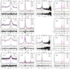 |
Fig. A.1. Spectral fits of (from top to bottom) Mrk 335, Mrk 110, Mrk 509, and Ark 564 in the wavelength ranges considered, with specific fluxes measured in units of 10−15 erg s−1 cm−2 Å−1 and the wavelength measured in Å. A lower box describing the residuals is associated with each spectral fit, with the wavelength expressed in units of radial velocities (km s−1). The original spectrum is plotted with a black line and the modeled spectrum is plotted in magenta. Each additional line component is plotted with a different colour, according to the legend. Dashed vertical lines represent the rest-frame wavelengths of the main lines of the selected spectral range. Left: λ1320-1450 Å range. Middle left: λ1450-1700 Å range. Middle right: λ1800-2100 Å range. Right: λ4430-5300 Å range. |
Appendix B: Distribution of U, nH, and Z for each object
The distribution of the physical parameters of U, nH, and Z for the 14 objects in our sample is shown in Figures B.1-B.5.
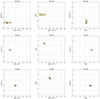 |
Fig. B.1. Two-dimensional parameter spaces illustrating the physical conditions of the gas in the BLR of the objects. Each plot represents the BC, with a green dot indicating the minimum χ2 computed between measured diagnostic ratios and CLOUDY simulations. The orange region corresponds to a 1σ accuracy. Blue and red dots and shades represent the minimum χ2 and associated regions for the BLUE and VBC, respectively. Left: Logarithmic plane of nH and Z. Middle: Logarithmic plane of nH and U. Right: Logarithmic plane of U and Z. |
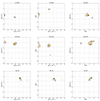 |
Fig. B.2. Continued. |
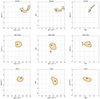 |
Fig. B.3. Continued. |
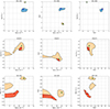 |
Fig. B.4. Continued. |
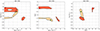 |
Fig. B.5. Continued. |
Appendix C: Results for individual sources
Here follow considerations on the results obtained for each of the individual sources.
C.1. Mrk 335
Mrk 335 is a Pop. A object. It has been a target of several reverberation mapping campaigns in the optical (Peterson et al. 2004): Grier et al. (2012) obtain 13.9 ± 0.9 days for Hβ. The resulting MBH is (2.6 ± 0.8)×107 M⊙, for a luminosity ≈7.7 ⋅ 1044 erg s−1. Mrk 335 is therefore considered a Pop. A source radiating at a modest Eddington ratio (Lbol/LEdd ≲ 0.2).
(although see Mastroserio et al. 2020). Its BLR was spatially resolved in the infrared, obtaining an upper limit for its size of 0.155 pc (GRAVITY Collaboration 2020). The source might presently be close to its lowest state (Grupe et al. 2018), although there has been a recent upturn (Komossa et al. 2020). Both CIV and Hβ do not reveal any significant blueshifted excess to the Lorentzian profile (cf. van Groningen 1987), implying a very weak wind component.
The estimation of the physical conditions in the BLR yielded a result characterized by a subsolar metallicity and a very low density. The low metallicity reported in the paper is a lower limit since the result is likely due to the lack of CLOUDY simulations with 0.2 Z⊙ or 0.5 Z⊙ (the Z of Mrk 110 and 509, with similar spectra, is around solar). Additionally, the gas density value is the lowest in the sample (log nH ∼8 cm−3). A low-density value is supported by very strong CIII] emission and a very low AlIII/CIII] ratio. Interestingly, the [O III]λλ4959,5007 doublet can be fit by an NC with a semi-BC with a width similar to the one of HβBC. The estimated BLR density is higher than the critical density of [O III]λλ4959,5007. However, some [O III]λλ4959,5007 emission is predicted by CLOUDY simulations to be ∼0.05 that of Hβ in the BLR. Considering the low BLR nH, a radial stratification of nH (Baldwin et al. 1995) may facilitate [O III]λλ4959,5007 emission.
C.2. Mrk 110
Mrk 110 is a Pop. A object of spectral type A1 that, not surprisingly, exhibits spectral features remarkably similar to Mrk 335. A peculiarity is the presence of a weak asymmetry toward the red in the profiles of both CIV and Hβ. The asymmetry was modeled, adding a faint redshifted component affecting CIV intensity by about 20%, with no significant effect on the Hβ flux. A redshifted asymmetry had already been detected in the Balmer, HeI, and HeIIλ4686 lines and has been interpreted as being due to gravitational redshift (Kollatschny et al. 2004; Müller & Wold 2006; Gavrilović et al. 2007). Consistently, the BLR of Mrk 110 appears to be compact: τ ≈ 20 − 30 ld (Peterson et al. 1998; Kollatschny et al. 2001; Li et al. 2013). If the MBH ≈2 ⋅ 107 M⊙ derived by Kollatschny et al. is corrected for a viewing angle of θ ≈ 30°, the central mass could reach ∼108. A photoionization solution following the locally optimized cloud model indicates emission from the BLR region starting at log r ≈ 15.3 (Juráňová et al. 2024), implying an inner radius of ∼100 gravitational radii. Gravitational and transverse shifts could then explain the shift amplitude of the additional components of CIV and Hβ included in the fit (≈4500 km s−1). If this interpretation is correct, the compact BLR and an overmassive black hole compared to other A1 sources could be at the origin of the redshifted excess (Gavrilović et al. 2007; Marziani 2023).
The CIV/Hβ ∼37 was deemed inappropriate, and thus excluded from the measurement of the metallicity. Indeed, similar measurements of the intensity of the lines from Juráňová et al. (2024) returned a value of ∼13, which is much more appropriate, indicating a light loss in our optical spectrum as being a possible cause of the mismatch. The solution obtained is very well constrained around solar metallicity (Fig. B.1, Tab. 8).
C.3. Mrk 509
Mrk 509 is a Pop. A1 object, with very weak or absent FeII lines in its optical spectrum. It has been monitored in the optical, UV, and X-ray domains (Kriss et al. 2019), and more recently in IR (Mitchell et al. 2024). Any blueshifted excess is barely visible in SiIV+OIV] and HeIIλ1640, and very faint in both CIV and Hβ, although spectropolarimetry reveals the presence of an accretion disk wind (Lira et al. 2021). Hβ reverberation mapping yields a time delay of ≈ 79.6 ld (Bentz et al. 2013; Du et al. 2015) and a mass ∼2 ⋅ 108 M⊙ (Yu et al. 2020). Additionally, its BLR was recently spatially resolved in the infrared, revealing an upper limit to its size of 0.249 pc (GRAVITY Collaboration 2020).
Measurement of the intensity of its lines, especially CIV and SiIV+OIV], has been affected by the presence of many absorption lines. However, the measured line ratios constrain Z, U, and nH very well, yielding a metallicity around the solar one, a value that could be considered typical of spectral type A1.
C.4. Ark 564
Ark 564 is a Pop. A object belonging to the A2 spectral bin of the MS. Long-term monitoring of the object has been performed over time in the optical range (Shapovalova et al. 2012), yielding a rather short time delay between continuum and Hβ variation, around 6.7 ± 10 days. There is evidence of excess emission on the blue side of the of CIV and HeIIλ1640 and high ionization. The relativistic wind has been detected in the X-ray domain via the discovery of lines of highly ionized oxygen shifted by ∼0.1c (Gupta et al. 2013). These properties are fairly typical of A2 sources with quite strong FeII emission and higher L/LEdd compared to the objects of spectral type A1.
The ionization parameter is consistent with log U ∼ −1 and the presence of strong CIII] emission drives the solution toward low-density values of log nH ∼7, as in the case of Mrk 335. Repeating the estimation of the physical parameters without the use of the diagnostic ratios including C III] returned a somewhat different scenario, with a higher density (log nH ∼ 11) and a solar metallicity, in better agreement with the reverberation delay (see the discussion in Section 6.4). The rather high χ2 value (Tab. 8) is due to the contributions of CIV/He IIλ1640 and CIII]/CIV, which are in turn due mainly to the small uncertainties associated with these two ratios, rather than to a disagreement between the observed and predicted values from the minimum χ2 solution (CIV/He IIλ1640 ≈ 4.3 vs. 2.9, and CIII]/CIV ≈ 0.87 vs. 0.57, predicted vs. observed). The result obtained for the metallicity, 5 Z⊙ is thus stable, including compared to other Pop. A objects. A detached 1σ region (Fig. B.1) would imply a slightly lower Z and a significantly higher nH (log nH ∼ 10 [cm−3]).
C.5. Mrk 478
Mrk 478 is a Pop. A object, an NLSy1 with prominent but not extreme FeII emission. A very recent study indicates an Hβ lag of ≈45 − 55 days to continuum changes (Woo et al. 2024). Not unlike Ark 564, Mrk 478 could be regarded as a bridge between the A1 and xA spectral types, since it exhibits some spectral characteristics that are typical of both. Its RFeII ∼ 1 makes Mrk 478 a borderline source (Marziani et al. 2010, see also Table 7). The high Z value obtained, along with U and nH, are plausible given our measurements. A relevant question is what drives the metallicity to a value that is higher by a factor of ten in an object that is not so dissimilar in the optical spectral range to Ark 564. As a matter of fact, CIV/HeIIλ1640, SiIV+OIV]/CIV, and SiIV+OIV]/He IIλ1640, all Z indicators, are ≈2.8, 2.4, and 6.5 times higher in Mrk 478. The SiIV+OIV]/CIV close to unity requires, under the physical conditions of the BLR, very high Z ∼ 𝒪(100) (Śniegowska et al. 2021; Garnica et al. 2022). The high χ2 (actually the highest of the sample) is due to the FeII/Hβ ratio: the predicted value is too low, by a factor of three. As in the case of Ark 564, the high intensity of CIII] measurement returns a lower gas density compared to that obtained for other xA sources. The relatively low density and high ionization are not conducive to strong FeII emission, but the observed prominence of FeII is certainly consistent with a high metallicity solution. Adding a microturbulence of 10 km s−1 to the estimation of the physical conditions retrieves a solution that has a very high χ2(≈170), and with a low density and a high metallicity (Z ∼ 200Z⊙). Indeed, the borderline characteristics of this object do not completely align with the extreme conditions that characterize xA sources, making this determination uncertain, and the previous one without microturbulence more reliable.
C.6. Ton 28
Even if the RFeII is not as high, Ton 28 shares several extreme properties with I Zw 1, such as extreme blueshifts in both CIV and [O III]λλ4959,5007 (Zamanov et al. 2002). Estimates of the time lag, τ, between continuum variations and the Hβ response are dependent on the method applied for the cross-correlation analysis; the Javelin-based (Zu et al. 2011) estimate is  ld, larger than the CCF centroid,
  ld (Li et al. 2021), consistent with a previous estimate affected by a large uncertainty (
 ld, Du et al. 2018). Velocity-resolved reverberation maps of Hβ reveal a signature of a Keplerian disk-like motion (Li et al. 2021). Spectropolarimetric observations indicate a large Hα line width in polarized light (≈4220 km s−1) compared to the width in natural light (≈1770 km s−1, Capetti et al. 2021), implying an almost face-on view (θ ≈ 15°, Śniegowska et al. 2023). Despite the lower S/N compared to other sources used in this work, the results obtained during the estimation of physical parameters are well constrained and suggest a solution of ≈50Z⊙, with a high density. Adding a microturbulence of 10 km s−1 to the estimation of the physical conditions, the results point to a solution of Z ∼ 20Z⊙, with a similar density and U to what there would be without microturbulence.
C.7. LB 2522
LB 2522 ≡ PG 1259+593 represents a typical xA object in our sample (Negrete et al. 2018), belonging to the A3 spectral type. LB 2522 has been subject to a reverberation study in the MIR wavelength range (Lyu et al. 2019) that yields a delay time in the W2 band1 of τ ≈ 794 days. These values set an upper limit for rBLR, with the delay time of the Hβ emission being estimated as being around τ = 225 ± 75 days (Du, private communication).
Although it is one of the most luminous objects in the sample, due to its large distance its FOS spectra are subject to more noise (S/N ≈ 5) than other sources studied in this work. Nevertheless, the line intensity yielded a fairly precise measurement of the physical parameters of the BLR, with a metallicity of about 20 Z⊙ and an average gas density (Tab. 8, Fig. B.3). After adding a microturbulence of 10 km s−1 to the estimation of the physical conditions, the results point to a solution of a similar metallicity, density, and U to what there would be without microturbulence.
C.8. LEDA 51016
LEDA 51016 ≡ PG 1415+451 is a typical xA object, exhibiting a very strong FeII emission in the optical wavelength range, and a prominent BLUE in CIV, which is also appreciable in Hβ (Fig. A.2). Optical monitoring for reverberation mapping yields a time delay of Hβ to continuum at 5100 Å of  days (Hu et al. 2021), to be compared with τ ≈ 433 days in the MIR (Lyu et al. 2019).
The COS and FOS spectra of LEDA 51016 appear with very high S/N, and the results are consistent with other xA sources of the sample, including a well-constrained supersolar metallicity ( ) and a relatively high gas density. In this case, as for the prototypical source I Zw 1, the low-ionization, high-density solution retrieved by Negrete et al. (2012) is possible within the 1σ uncertainty range (Tab. 8, Fig. B.2). Adding a microturbulence of 10 km s−1 to the estimation retrieves a similar solution as that without microturbulence, but with a slightly lower metallicity (Z ∼ 10Z⊙).
C.9. I Zw 1
I Zw 1 is a narrow-line Seyfert 1 galaxy with a strong FeII emission (Phillips 1978). Emission lines are narrow, with Hβ FWHM estimates in the range between 1100–1500 km s−1. The line narrowness has made I Zw 1 an ideal source for the extraction of a template of FeII emission in the optical (Boroson & Green 1992; Laor et al. 1997b; Marziani et al. 2009), IR (Garcia-Rissmann et al. 2012), and UV (Vestergaard & Wilkes 2001) domains. The source has been hailed as a prototype for Pop. A (Sulentic et al. 2000a) and, more recently, for extreme Pop. A (Marziani & Sulentic 2014), due to its strong FeII, weak C III], high SiIV+OIV]/CIV ratio, and weak CIV equivalent width. I Zw 1 has been monitored for reverberation mapping: the rest-frame delay for Hβ is  days (Huang et al. 2019). More recently, the amplitude of flux variation has been so small as to make impossible to estimate a time lag for Hβ (U et al. 2022).
Previous studies focused on the physical conditions in the virialized BLR of I Zw 1 suggested a low-ionization solution, with a high density (Marziani et al. 2010; Panda 2021b) and a possible metallicity enhancement (Negrete et al. 2012). The estimation of the physical parameters in this work leads to a solution of ≈20Z⊙, with medium-high density. Adding a microturbulence of 10 km s−1 to the estimation retrieves a similar solution with a metallicity of Z ∼ 20Z⊙.
C.10. PHL 1092
PHL 1092 has been hailed as one of the strongest FeII emitters ever discovered (Marinello et al. 2020; Panda et al. 2020; Martínez-Aldama et al. 2021, and references therein). Our measurements confirm the extremely strong RFeII ≈1.75 placing PHL 1092 in the spectral type A4, where only ≈3% of optically selected quasars are found (Marziani et al. 2013). The measurements of line intensities and FWHM for the BC and BLUE in both the optical and UV ranges are consistent with those reported in Marinello et al. (2020) (the slightly higher value of RFeII reported by these authors is due to their removal of the BLUE of Hβ). The extreme attributes of this object are highlighted by its distinction as the sole source in the sample displaying a BLUE in the λ1900 blend, a rare occurrence even among xA objects (Marziani et al. 2022; Buendia-Rios et al. 2023).
The metallicity estimated for this source (Z ∼ 1000Z⊙) is apparently out of scale, higher than the highest estimates for xA quasars at high luminosity, which seldom exceed Z ∼ 100Z⊙ (Garnica et al. 2022). However, this result aligns with the low-ionization, high-density solution of xA sources (Negrete et al. 2012): low CIV, high AlIII/SiIII], high SiIV+OIV]/HeIIλ4686, prominent FeII, and very low CIII]/SiIII] imply low U, high nH, and high Z. The inordinately high value of Z is driven by SiIV+OIV]/CIV ≳1, which excludes Z values only a few times higher than the solar one. In the case of PHL 1092, the CIV/HeIIλ4686 and CIV/Hβ ratios are highly uncertain, in part because of absorptions. The ionization parameter of ∼10−3 accounts for the weak CIV: the CIV BC equivalent width is just ≲ 2 Å, with a CIV/Hβ ratio of ∼1. The W CIV BC+BLUE ≈ 8 Å, qualifies PHL 1092 among the weak-lined quasars (WLQs; Diamond-Stanic et al. 2009; Shemmer et al. 2010; Shemmer & Lieber 2015), which are xA sources by a wide majority (Marziani et al. 2016; Martínez-Aldama et al. 2018).
The out-of-scale value of Z ∼ 1000Z⊙ is greatly reduced to  Z⊙ if a microturbulence ≈ 10 km s−1 is introduced in the computations, which acts as a metallicity controller (see Panda 2021b, for an in-depth analysis). A major difficulty is introduced by the large errors associated with most measured ratios (Tab. 7), and accounts for the wide uncertainty range. Therefore, the metallicity estimated for the BLUE (Z ∼ 50Z⊙) could provide a representative lower limit for this object, since it accounts for most of the observed flux in the HILs. BLUE and the BC revision with turbulence will still place the source on par with the highest Z estimates in the sample. Indeed, estimating the physical conditions for the BC of this source introducing the effects of 10 km s−1 microturbulence leads to the greatest changes in physical conditions for any object in the sample, with log nH ∼11 cm−3 and
  , in addition to the aforementioned change from Z ∼ 1000Z⊙ to Z ∼ 50Z⊙. The large uncertainties leave open the possibility of a low-ionization, high-density solution, like that envisaged by Negrete et al. (2018) for the xA sources. The addition of microturbulence in the estimation of the physical parameters is further discussed in Section 5.5.
C.11. Fairall 9
Fairall 9 is a prototypical Pop. B source, with its spectrum almost coinciding with the composite spectrum of Pop. B objects (Jiang et al. 2021, M23). Reverberation mapping of the object has been performed in the past in the optical, yielding a well-defined delay of  days (Bentz et al. 2013). Dust-reverberation mapping yielded a delay in the W1 and W2 maps ≈ 250 days in the W1 band at 3.4μm, and between ≈280 and ≈370 days for the W2 band at 4.6 μm (Chen et al. 2023). The Fairall 9 Hβ red wing extends up to ∼18, 000 km s−1, beyond [O III]λλ4959,5007 (Fig. A.3). This is not uncommon among Pop. B sources. The only peculiarity is the occurrence of a plateau on the red side of Hβ NC, leaving a faint semi-broad residual at vr ≈ 2500 km s−1. Analogous features are seen in Pop. B objects, albeit rarely. One case in point is Ark 120, discussed below. A spectropolarimetric analysis of Fairall 9 (Jiang et al. 2021) suggested the presence of a warped geometry of the accretion disk, but it is not obvious if the residual feature detected in natural light is connected to the warped disk.
The estimations of the metallicity of the BC and VBC return about 2 Z⊙ for the BC and 1 Z⊙ for the VBC, which is consistent within the uncertainties (Fig. B.3). The 1σ confidence range of Z for the BC is rather broad, ranging from -1 to 0.7. The ionization parameter is constrained within an order of magnitude, and the nH is only within four orders of magnitude. The VBC parameters appear better constrained. The wide range of confidence intervals might be an indication of radial stratification in the BLR gas emitting the BC. The VBC, as it is associated with gas in the innermost region, may have intrinsically better-defined physical parameters.
C.12. Ark 120
Ark 120 stands out as the most peculiar object in the sample. The main peculiarity is its unusual double-peaked Hβ profile, which was modeled in this work using a BC and two satellite components, one blueshifted and the other redshifted, roughly symmetrically displaced by ±2000 km s−1. This profile is not unique, and likely hints toward some reproducible structure or dynamical process within the BLR (Marziani et al. 1992; Korista 1992; Korista et al. 1997). Even after extensive monitoring, the nature of its double-peaked profile has not been completely understood, although periodic variations have been suggested (Li et al. 2019). Fairall 9 might undergo a similar phenomenon.
Ark 120 exhibits a rather strong FeII emission for a Pop. B object (RFeII = 0.84, see Table 7), likely originating in a region further from the one in which originates Hβ, which exhibits a time delay of τ = 57.3 ± 23.0 days (Kuehn et al. 2008).
The presence of a mismatch between the UV and optical fluxes after correcting the flux for galactic extinction indicates the presence of a stronger extinction than expected. This leads to an underestimation of the CIV/Hβ ratio, which reduces the resulting metallicity. We therefore excluded the C IV/Hβ diagnostic ratio during the computation. Once excluded from the inordinately low CIV/Hβ, the Z solution converges to a well-defined metallicity value. The moderate SiIV+OIV]/CIV ratio indicates abundances at least the same as the solar one or a few times higher than it. The value obtained (Z ∼ 10Z⊙) for the BC is consistent with the one for the VBC (Z ∼ 5Z⊙). This is in the case that the satellite lines are included in the total flux of the BC. Removing them, and using only the central core of the Hβ profile (Fig. A.4), would imply an RFeII ≈1.5 that is out of scale to the other line ratios.
C.13. NGC 3783
NGC 3783 is the closest object of the sample, located at a redshift of z = 0.009. It is a well-known object, extensively monitored for reverberation mapping, with an Hβ-emitting region having a median radius delay of  lt-day (Bentz et al. 2021). Lira et al. (2021) performed a spectropolarimetric study of the object, revealing evidence of a nuclear wind whose presence is also revealed by the excess of the blue side of CIV and SiIV+OIV] (Fig. A.4), most likely due to outflowing gas. The BLR of NGC 3783 was spatially resolved in the infrared, obtaining an upper limit for its size of 0.110 pc (GRAVITY Collaboration 2020). The spectrum of this object almost coincides with the composite spectrum obtained for the RQ Pop. B.
Confronting the diagnostic ratios of the analyzed spectra with the CLOUDY simulations, the BC is associated with a slightly subsolar metallicity, with the VBC having a compatible result of solar metallicity. The ionization parameter gradient obtained for the BC and VBC of this object is consistent with a more ionized VBC, being closer to the ionizing source.
All Tables
All Figures
|
Fig. 1. Stacked histograms depicting the distribution of sample objects in log(Lbol) and z, categorized by the respective population. Assigned colors correspond to the legend, while vertical lines denote average values from the objects used in the referenced works S21, G22, and M23. |
| In the text | |
|
Fig. 2. Behavior of the diagnostic ratio, C IV/Hβ, (shown on a logarithmic scale) as a function of the ionization parameter, U, and metallicity, Z, for four values of hydrogen density, log nH = 7,9,11,13 [cm−3], using the Mathews & Ferland (1987) Pop. A SED. |
| In the text | |
|
Fig. 3. Left: plot of the χ2/χmin2 distribution as a function of the relative intensity of the FeIIBC of PHL 1092 with respect to the specfit retrieved intensity, vs. the relative intensity of the FeIIBLUE with respect to the original intensity of FeIIBC. Middle: same, but for the AlIIIVBC emission of Fairall 9. Right: same, but for the FeIIVBC emission of Fairall 9. |
| In the text | |
|
Fig. 4. MS representation of our sample. Every object is placed according to its RFeII and FWHM(Hβ). Greater metallicity, Z, is expressed with increasing marker sizes and different colors. Objects with subsolar metallicity are marked in red, objects with 1 Z⊙ ≤ Z ≤ 2 Z⊙ in orange, objects with 2 Z⊙ < Z ≤ 10 Z⊙ in gold, objects with 10 Z⊙ < Z ≤ 50 Z⊙ in blue, and objects with metallicity greater than 50 Z⊙ in indigo. Sources from this work are shown in circles. Squares are used as reference values for the objects in S21, G22, and M23, the latter with two squares, one for RL sources and the other for RQ sources. The gray region describes the typical positions occupied by objects along the MS (Zamfir et al. 2010; Garnica et al. 2022). |
| In the text | |
|
Fig. 5. Median Z values for 200 replications of the intensity ratios deviating from the ones predicted by four models as a function of fractional uncertainties. |
| In the text | |
|
Fig. 6. Two-dimensional parameter space of log Z − log U illustrating the physical conditions of the gas surrounding xA sources with different SEDs. In each plot, the minimum χ2 computed between measured diagnostic ratios and CLOUDY simulations is shown with dots: green for the Mathews & Ferland (1987) SED and blue for the xA SED. The orange region corresponds to the 1σ accuracy range for the Mathews & Ferland (1987) SED, and the blue region for the xA SED. |
| In the text | |
|
Fig. 7. Behavior of the diagnostic ratio CIV/He IIλ1640 (magenta), CIV/Hβ (blue), RFeII (green) on a logarithmic scale vs. microturbulence velocity in km s−1. Left: using the solution for I Zw 1 (squares) and PHL 1092 (circles). Right: Using a low-ionization, high-density solution appropriate for xA sources (see text for details), with three different Z values: 200 Z⊙ (circles), 100 Z⊙ (squares), and 50 Z⊙ (triangles). |
| In the text | |
|
Fig. 8. Diagram illustrating the trend of Z across different spectral types, with the reference values for each spectral type obtained as the geometric mean of all the measurements assumed for all the objects belonging to a specific spectral type, including our method, the use of the CIV/Hβ ratio, and the presence of microturbulence for all sources belonging to the A2, A3, and A4 spectral types. Confidence intervals are obtained as the standard deviation of our results. The number of objects contributing to each spectral type is shown in green, along with the average RFeII of the sources considered. Two reference points (in red) are shown describing the RL and RQ Pop. B sources studied in M23. |
| In the text | |
|
Fig. 9. Figures showing a correlation between various accretion parameters with log Z and RFeII. Points are displayed using the same color-coding as in Figure 4, with their error bars. When the correlation is considered significant (rP ≳ 0.7, corresponding to a confidence level of ≈0.01), the correlation line is shown, with its defining parameters intercept (A) and slope (B) shown with their respective errors. For each correlation are also shown the Pearson correlation coefficient, rP, from the SLOPES program (Feigelson & Babu 1992) and the probability, P, of a spurious correlation. |
| In the text | |
|
Fig. 10. Top: scatter plot showing the comparison of rBLR estimated with reverberation mapping (rBLR, RM), and using CLOUDY photoionization simulations (rBLR, Φ), on a logarithmic plane. Points are displayed using the same color-coding as in Figure 4, with their respective error bars. The dash-dotted line describes the position of objects for which the two independent determinations coincide. The values of rBLR, Φ for objects whose determinations do not coincide with rBLR, RM by a margin are shown in the upper right quadrant of the figure (expressed in pc), connected to their representative points through an arrow. An alternative result of the determination of physical parameters is shown for Ark 564 with a square, obtained by removing the diagnostic ratios employing CIII]. Bottom: plot showing the difference between the two estimations. The horizontal dash-dotted line describes the position of objects for which the two independent determinations coincide. The dotted line connects the two different determinations for Ark 564 described above. |
| In the text | |
|
Fig. A.1. Spectral fits of (from top to bottom) Mrk 335, Mrk 110, Mrk 509, and Ark 564 in the wavelength ranges considered, with specific fluxes measured in units of 10−15 erg s−1 cm−2 Å−1 and the wavelength measured in Å. A lower box describing the residuals is associated with each spectral fit, with the wavelength expressed in units of radial velocities (km s−1). The original spectrum is plotted with a black line and the modeled spectrum is plotted in magenta. Each additional line component is plotted with a different colour, according to the legend. Dashed vertical lines represent the rest-frame wavelengths of the main lines of the selected spectral range. Left: λ1320-1450 Å range. Middle left: λ1450-1700 Å range. Middle right: λ1800-2100 Å range. Right: λ4430-5300 Å range. |
| In the text | |
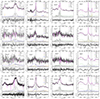 |
Fig. A.2. Same as in Figure A.1 but for Mrk 478, Ton 28, LB 2522, and LEDA 51016, respectively. |
| In the text | |
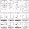 |
Fig. A.3. Same as in Figure A.1 but for I Zw 1, PHL 1092, Fairall 9, and Ark 120, respectively. |
| In the text | |
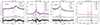 |
Fig. A.4. Same as in Figure A.1 but for NGC 3783 |
| In the text | |
|
Fig. B.1. Two-dimensional parameter spaces illustrating the physical conditions of the gas in the BLR of the objects. Each plot represents the BC, with a green dot indicating the minimum χ2 computed between measured diagnostic ratios and CLOUDY simulations. The orange region corresponds to a 1σ accuracy. Blue and red dots and shades represent the minimum χ2 and associated regions for the BLUE and VBC, respectively. Left: Logarithmic plane of nH and Z. Middle: Logarithmic plane of nH and U. Right: Logarithmic plane of U and Z. |
| In the text | |
|
Fig. B.2. Continued. |
| In the text | |
|
Fig. B.3. Continued. |
| In the text | |
|
Fig. B.4. Continued. |
| In the text | |
|
Fig. B.5. Continued. |
| In the text | |
Current usage metrics show cumulative count of Article Views (full-text article views including HTML views, PDF and ePub downloads, according to the available data) and Abstracts Views on Vision4Press platform.
Data correspond to usage on the plateform after 2015. The current usage metrics is available 48-96 hours after online publication and is updated daily on week days.
Initial download of the metrics may take a while.