| Issue |
A&A
Volume 667, November 2022
|
|
|---|---|---|
| Article Number | A105 | |
| Number of page(s) | 50 | |
| Section | Extragalactic astronomy | |
| DOI | https://doi.org/10.1051/0004-6361/202142837 | |
| Published online | 11 November 2022 | |
High metal content of highly accreting quasars: Analysis of an extended sample
1
Instituto de Astronomía, UNAM, Mexico City 04510, Mexico
2
CONACyT Research Fellow – Instituto de Astronomía, UNAM, Mexico City, 04510, Mexico
e-mail: alenka@astro.unam.mx
3
National Institute for Astrophysics (INAF), Padova Astronomical Observatory, 35122 Padova, Italy
4
Nicolaus Copernicus Astronomical Center, Polish Academy of Sciences, ul. Bartycka 18, 00-716 Warsaw, Poland
5
Center for Theoretical Physics, Polish Academy of Sciences, Al. Lotników 32/46, 02-668 Warsaw, Poland
6
Laboratório Nacional de Astrofísica – MCTIC, R. dos Estados Unidos, 154 – Nações, Itajubá, MG 37504-364, Brazil
Received:
5
December
2021
Accepted:
27
July
2022
Context. We present an analysis of UV spectra of quasars at intermediate redshifts believed to belong to the extreme Population A (xA), aimed to estimate the chemical abundances of the broad line emitting gas. We follow the approach described in a previous work, extending the sample to 42 sources.
Aim. Our aim is to test the robustness of the analysis carried out previously, as well as to confirm the two most intriguing results of this investigation: evidence of very high solar metallicities and a deviation of the relative abundance of elements with respect to solar values.
Methods. The basis of our analysis are multicomponent fits in three regions of the spectra centered at 1900, 1550, and 1400 Å in order to deblend the broad components of AlIIIλ1860, C III]λ1909, CIVλ1549, He IIλ1640, and SiIVλ1397+OIV]λ1402 and their blue excess.
Results. By comparing the observed flux ratios of these components with the same ratios predicted by the photoionization code CLOUDY, we found that the virialized gas (broad components) presents a metallicity (Z) higher than 10 Z⊙. For nonvirialized clouds, we derived a lower limit to the metallicity around ∼5 Z⊙ under the assumption of chemical composition proportional to the solar one, confirming the previous results. We especially relied on the ratios between metal lines and He IIλ1640. This allowed us to confirm systematic differences in the solar-scaled metallicity derived from the lines of Aluminum and Silicon, and of Carbon, with the first being a factor ≈2 higher.
Conclusions. For luminous quasars accreting at high rates, high Z values are likely, but Z-scaled values are affected by the possible pollution due to highly-enriched gas associated with the circumnuclear star formation. The high-Z values suggest a complex process involving nuclear and circumnuclear star formation and an interaction between nuclear compact objects and an accretion disk, possibly with the formation of accretion-modified stars.
Key words: galaxies: active / quasars: emission lines / quasars: supermassive black holes / line: profiles / galaxies: abundances
© K. Garnica et al. 2022
 Open Access article, published by EDP Sciences, under the terms of the Creative Commons Attribution License (https://creativecommons.org/licenses/by/4.0), which permits unrestricted use, distribution, and reproduction in any medium, provided the original work is properly cited.
This article is published in open access under the Subscribe-to-Open model. Subscribe to A&A to support open access publication.
1. Introduction
The diversity of broad-line quasars has been efficiently organized through the parameter space of Eigenvector 1 (E1) in several studies during the last three decades (Boroson & Green 1992; Sulentic et al. 2000a; Shen & Ho 2014). Sulentic et al. (2000a,b, 2007) proposed an E1 space that is represented by four dimensions (4DE1) with two spectroscopical parameters defining an optical plane: 1) FWHM(Hβ), the full width at half maximum of the Hβ broad component; and 2) RFeII = F(FeIIλ4570)/F(Hβ), the ratio of the optical FeII emission between 4434 Å and 4684 Å to the Hβ intensity. The two remaining parameters involve spectral measurements in the UV and X-ray observations: 3) CIV c(1/2), the centroid line shift of CIV; and 4) Γsoft, the soft X-ray photon index.
The observed pattern in the optical plane of the 4DE1 (FWHM(Hβ) vs. RFeII) has been identified as the quasar main sequence (MS) since it is associated with trends of physical properties such as the mass of the supermassive black hole (MBH), the broad-line region (BLR) gas density (nH), the ionization parameter (U), and the Eddington ratio (L/LEdd, Boroson & Green 1992; Boroson 2002; Panda et al. 2018, 2020b; Wildy et al. 2019). However, the principal driver of the MS is probably the Eddington ratio (Boroson & Green 1992; Marziani et al. 2001; Sun & Shen 2015), which is a basic parameter that expresses the balance between radiation and gravitational forces and is related to the structure of the accretion flow (Giustini & Proga 2019; D’Onofrio et al. 2021).
Two Populations, A and B, have been defined from this parameter space. They are delimited at 4000 km s−1, with Pop. B objects being the ones with the broadest widths (Sulentic et al. 2000a, 2009; Sulentic & Marziani 2015). However, although this condition subdivides quasars of different properties, spectral differences in objects in the same population can still be found, particularly in Population A (Fig. 2 of Sulentic et al. 2002; cf. Shen & Ho 2014). This is why a subdivision in bins of ΔFWHM(Hβ) = 4000 km s−1 and ΔRFeII = 0.5 was introduced. Bins A1, A2, A3, and A4 are defined in increasing RFeII, while bins B1, B1+, and B1++ are defined in increasing FWHM(Hβ) (see Fig. 1 of Sulentic et al. 2002; cf. Shen & Ho 2014). Sources of the same spectral type show similar spectroscopic measures (e.g., line profiles and UV line ratios, Bachev et al. 2004; Sulentic et al. 2007) and similar physical parameters.
Most interesting along the MS are the spectral types at the extremes (Marziani et al. 2021). At the high RFeII end, quasars are found to be radiating at a high Eddington ratio from a variety of theoretical and observational analyses (e.g., Marziani et al. 2001; Sun & Shen 2015; Du et al. 2016; Panda et al. 2019). High Eddington ratio quasars can be selected on the basis of empirical criteria based on the MS spectral types (e.g., Wang et al. 2013, 2014; Marziani & Sulentic 2014; Du et al. 2016). According to Marziani & Sulentic (2014, hereafter MS14), they are defined by having
that is to say, the flux of the FeIIλ4570 blend on the blue side of Hβ (as defined by Boroson & Green 1992) exceeds the flux of Hβ, and the spectral type is An with n ≥ 3. In the optical diagram of the quasar MS (Sulentic et al. 2000b; Shen & Ho 2014; Marziani et al. 2018), they are at the extreme tip in terms of Fe II prominence and identified as extreme Population A (hereafter xA).
At relatively modest redshifts (z ≳ 1), the Hβ line is already shifted into the NIR. Since NIR spectroscopic observations are still difficult, it is expedient to resort to the quasar-rest frame UV spectrum shifted into the visual range. For z ≳ 1, the criteria for selecting xA objects based on two UV line intensity ratios are believed to be satisfied:
![$$ \begin{aligned}&\frac{F(\mathrm{AlIII} \lambda 1860)}{F(\mathrm{SiIII]} \lambda 1892)}\ge 0.5\nonumber \\&\frac{F(\mathrm{SiIII]} \lambda 1892)}{F(\mathrm{CIII]} \lambda 1909)} \ge 1.0, \end{aligned} $$](/articles/aa/full_html/2022/11/aa42837-21/aa42837-21-eq2.gif)
following MS14. These criteria are believed to be met by the sources satisfying the condition of Eq. (1).
There have been previous claim of very high metallicity needed to account for the extreme Fe II emission (Panda et al. 2018, 2019; Panda 2021) as well as to account for the metallicity-sensitive UV emission line ratios (Baldwin et al. 2003; Warner et al. 2004; Shin et al. 2013; Sulentic et al. 2014). The aim of this work is to investigate the metallicity-sensitive diagnostic ratios of the UV spectral range for an extended sample of extreme Population A quasars that is for highly accreting quasars, capitalizing on the recent developments by Śniegowska et al. (2021, hereafter S21). At variance with previous work, S21 relied on (1) the decomposition of the emission line profiles in a broad component, symmetric at rest frame, and a BLUE component associated with the prominent blueshifted excess observed in high-ionization lines of these sources (e.g., Sulentic et al. 2017; Martinez-Aldama et al. 2018), and (2) the use of diagnostic intensity ratios involving metal lines and HeIIλ1640.
In the present work, we extend the method of S21 to a larger sample of xA quasars (Sect. 2). In Sect. 3, we describe the methodology used. Results on the 42 objects are provided in Sect. 4. They include the measurements on the fit of the emission blends (Sect. 4.1), along with the estimates of the metal content for fixed physical conditions and for ionization and density free to vary. The discussion of the results (Sect. 5) is mainly focused on the test of the stability of the method with two fitting techniques and of one of the main results of S21, namely that metallicity values derived from the diagnostic ratios are not consistent with scaled solar abundance ratios.
2. Sample
2.1. Sample definition
The xA sources considered in this study have rest-frame UV spectra from SDSS DR12 with coverage of 1000–3000 Å where we can find: (1) the strongest high ionization lines (HILs) associated with resonance transitions (e.g., SiIVλ1397, C IVλ1549), (2) usually weak low ionization lines (LILs; e.g., Si IIλ1814), and (3) several inter-mediate ionization lines (IILs) from transitions leading to the ground state (e.g., AlIIIλ1860, and the intercombination lines SiIII]λ1892, CIII]λ1909). For some of the spectra the blend Lyα + N Vλ1240 is present. As in the case of S21, measurements were discarded because of the strong absorptions alongside the emissions that make it difficult to interpret the blend.
The initial sample consisted of 526 objects with a redshift range centered at z = 1.5 − 2.2 from SDSS-DR12 to ensure moderate-to-high S/N in the continua. Based on a semi-automatic selection using the AlIII/SiIII] flux ratio as a high accretion rate indicator (MS14), the original sample was reduced to 120 objects. Subsequently we restricted the redshift range, centering it at z ≈ 2.2, so it would be possible to observe these objects in the H band and to obtain observations of Hβ in the infrared. This will give us the possibility of an eventual comparison of the indicators of accretion at different regions of the electromagnetic spectrum using different indicators. Finally, this restricts our sample to the 42 objects that are used in this work, all type-1 quasars, with 6 of them classified as Broad Absorption Line Quasars (BAL QSOs).
In summary, the 42 SDSS sources in this study are bright quasars (r < 19) with S/N from 10 up to 50 around 1400 Å. They are located between −11° < δ < 10° under a redshift coverage of 2.13 < z < 2.42. Each spectrum is similar to the other, except for a few outliers which will be analyzed in Sect. 5.
2.2. Sample properties
The basic properties of our sample are presented in Table 1: (1) SDSS name, (2) redshift from the SDSS, (3) the difference between our redshift estimation using Mg II and the SDSS redshift δz = z − zSDSS, (4) the g-band magnitude provided by SDSS Sky Server, (5) the g − r color index, (6) and (7) are the rest-frame specific continuum flux at 1700 Å and 1350 Å respectively, (8) the S/N ∼ 25 at 1450 Å, and (9) indicates the BAL QSOs and the objects from the S21 sample. Figure 1 and Table 1 indicate that the sources of our sample are very luminous, i.e., they are at the high-end of the luminosity distribution of BOSS sources at redshift z ≈ 2, and of rather homogeneous properties. As a consequence, we may not expect strong correlations with physical properties such as L, MBH, L/LEdd. The sample is best suited to confirm the main results seen by S21, and to improve their statistical significance. In addition, the scatter in the color index SIQR (semi interquartile range) is g − r ≈ 0.07 with a median g − r ≈ 0.27. This scatter suggests that the sample is not suffering strong extinction save SDSS J151636.79+002940.4 (g − r ≈ 1) and other sources with g − r ≈ 0.4 − 0.5 that are all BAL QSOs (BALQ). These sources were not considered in the analysis.
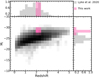 |
Fig. 1. Redshift distribution of the sample as a function of the absolute i-band magnitude Mi. The gray-scale squares show the Lyke et al. (2020) data, binned over small bins in z and Mi. The pink squares identify the sample used in this work. Upper panel: normalized redshift distribution. The pink histogram shows the corrected redshift adopted in this paper (see Sect. 3.1). Right panel: normalized absolute i-band magnitude distributions for both Lyke et al. (2020) and our sample. |
Source identification and basic properties.
3. Methods
This is the second paper in the series (the first being S21) with an extended sample, and therefore we follow the same basic methodology: (1) multi-component analysis of the emission blends in the UV spectra, (2) CLOUDY photoionization modeling and (3) metallicity estimates of the sample by comparing observed fluxes and CLOUDY synthetic fluxes at different U and nH values. The 13 sources from S21 are also presented in this article (identified in Col. 9 of Table 1) but they were reprocessed and refitted. A systematic comparison between the new measurements and the ones of S21 is carried out in Sect. 5.1.2.
3.1. Additional redshift determination
xA sources are characterized by a strong asymmetric blue-shifted component mainly in the regions centered at 1400 and 1550 Å (e.g., Sulentic et al. 2007, 2017; Vietri et al. 2018). These asymmetric emissions are frequently even stronger than the expected broad component emission. The peak of the line profile might therefore appear shifted by several thousands km s−1 (e.g., Hewett & Wild 2010). Even if the AlIIIλ1860 line is in most cases unshifted (within ±200 km s−1) with respect to the rest frame (Buendia-Rios et al. 2022), an excess component is occasionally present on the blue wing of the Al IIIλ1860 doublet causing a wrong measurement of the rest frame (Martínez-Aldama et al. 2017; Marinello et al. 2020; Marziani et al. 2022). Hence we estimate the redshift from the Mg IIλ2800 low-ionization emission line usually characterized by a symmetric line profile. Other spectral lines such as Si IIλ1814 or [OI]λ1304 are weak and are affected in some cases by low S/N or contaminated by absorptions lines. CIII]λ1909 and SiIII]λ1892 are heavily blended together. To improve the precision of the redshift estimate, we fit a Gaussian to top half of the Mg IIλ2800 line using the IRAF splot task to measure its central wavelength. Afterward we added a redshift correction to the original redshift from the Sloan when necessary using the IRAF dopcor task. These z corrections were up to 0.019 with respect to the SDSS redshift and affected more than two thirds of our sample (as shown in Col. 3 of Table 1) that guarantee us a better analysis of the data specially for the strong blue-shifted components at λ1400 and λ1550. The Mg IIλ2800 emission may however present a blue displacement less than 200–300 km s−1 (Marziani et al. 2013) that does not lead to any drastic misinterpretation of the line blends. We cross-checked the reshift obtained from Mg IIλ2800 with the one from the AlIII doublet broad component, and found consistency with the two z estimates.
3.2. Line interpretation and diagnostic ratios
As mentioned in Sect. 2, our spectral coverage is characterized by HILs, IILs and LILs. These emissions need a favorable environment for their associated transitions to occur, and in turn they provide insight on the gas surrounding the ionization source. Population A sources are characterized by broad components described with symmetric profiles plus strong asymmetric blue-shifted components associated with high-ionization emission (Leighly & Moore 2004; Marziani et al. 2010), hence we decomposed our regions of interest mainly using two emission profiles: 1) the broad component (BC), a rest-frame emission modeled with a Lorentzian profile. This symmetric profile is believed to be associated with a virialized system of clouds in the vicinity of the central supermassive black hole, and 2) the blue-shifted component (BLUE), a strong flux excess mainly in the blue wing of HILs that are resonance transitions, ultimately ascribed to high velocity winds. We modeled this emission with a very broad skewed Gaussian profile as an interpretation of the high velocity winds in which these emissions occur. The profiles of both BC and BLUE are constrained by the reduction to minimum χ2 on the full extent of the line.
3.2.1. Broad component
The analysis follows the same procedure of S21, and relies mainly on the ratios AlIII, CIV, SiIV + OIV] over He II. These ratios give us more direct information about the metal content even if He II is a weak emission mixed in the red wing of CIV. It might be underestimated and thus set an unrealistic upper limit for the metallicity. The issue will be discussed in Sect. 5.1.1.
In addition, we considered the line ratios (SiIV + OIV])/C IV, AlIII/CIV, and AlIII/SiIII]. The first ratio is frequently computed in metallicity studies of the BLR (Nagao et al. 2006b; Shin et al. 2013). The second one is more related to the possibility of AlIII overabundance, and the third one is associated with the selection of xA sources and is strongly dependent, for a fixed spectral energy distribution (SED), on both Z and nH (Marziani et al. 2020).
3.2.2. BLUE component
We measured BLUE components for three blends: the one at λ1400, mostly due to SiIV and OIV] emission, the ones for the CIV and He II at the 1550 Å region. We base our analysis on three ratios, with only two of them being independent: CIV/HeIIλ1640, (SiIV + OIV])/HeIIλ1640 and (SiIV + OIV])/CIV. We also sporadically measure a component on the blue side of AlIII, although we would not consider diagnostic ratios involving BLUE AlIII because this component shows a profile narrower than those of CIV, SiIV + OIV] and HeIIλ1640. Also, the measurement of AlIII BLUE intensity is uncertain, as it is affected by the Si IIλ1814 emission. Specific to the BLUE intensity ratios, we note that the (SiIV + OIV]) is often affected by heavy absorptions (even more than CIV) that may systematically lower the Z estimates from the ratio (SiIV + OIV])/HeIIλ1640.
3.3. Analysis via multicomponent fits
We analyzed our sample using the IRAF specfit task (Kriss 1994) to deblend the regions of interest centered at 1400, 1550 and 1900 Å in the SDSS spectra. These regions are a mix of emission lines (such as blue-shifted and broad components) and narrow absorption lines, making it necessary to obtain the best fit according to the minimum χ2 computed by a nonlinear multi-component fit. The Figures of the fit results for the full sample are shown in Appendix A, and an example is shown in Fig. 2. Each figure shows the continuum placement for the three regions (upper panels) and the fit of the blended lines with the appropriate components (lower panels). The regions of each spectra are fit separately, however imposing an overall consistency on the continuum shape.
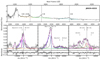 |
Fig. 2. SDSS J092919.45+033303.4, with specfit analysis results. Top panel: full spectrum as a function of rest-frame wavelength, after normalization at 1350 Å. The actual continuum ranges employed in the fitting of the three spectral regions discussed in the paper are marked. Bottom panels: decomposition of the blends. Black lines: observed spectrum under continuum subtraction. Magenta dashed lines: full model of the observed spectrum. Thick black lines: BC of SiIV, CIV, HeIIλ1640, AlIII and SiIII]. Blue lines: blue-shifted components of SiIV + OIV], CIV and HeIIλ1640. Green line: FeIII(UV34) template. Red line: CIII] emission. Gray lines: faint lines affecting the blends or AlIII BLUE component. |
Each region was analyzed according to Negrete et al. (2012). The components specific to the three spectral regions used are as follows:
1900 Å region:
– The continuum, modeled as a local power law using spectral windows free from lines at the edges of the emission regions to be analyzed;
– Broad components, AlIII doublet and SiIII] were modeled using symmetric Lorentzian profiles sharing the same FWHM, since both emissions have an ionization potential below 20 eV in most cases;
– CIII] emission, modeled using symmetric Lorentzian profiles with an independent FWHM;
– Fe III emission was modeled using a template from Bruhweiler & Verner (2008), with a maximum in the red wing of the 1900 Å blend;
– Fe II emission was found just for a third of the sample. A Fe II template could not model our data. We individually fit the emission at ≈1785 Å due to the Fe II multiplet UV 191 using a symmetric Gaussian profile;
– BLUE AlIII emission. Although the region emitting most AlIII is believed to be the virialized part of the BLR, we found evidence of outflows (i.e., excess blueshift with respect to the symmetric profile) in the blue wing of AlIII for 6 sources. This emission was modeled using a blue-shifted asymmetric Gaussian profile.
1550 Å region:
– The continuum, modeled as a local power law using spectral windows free from lines at the edges of the spectral region;
– Broad components of CIV and He II modeled with Lorentzian profiles sharing the same FWHM;
– BLUE components of CIV and He II were modeled with asymmetric Gaussian profiles sharing the same FWHM and displacement from the broad component. Blue-shifted emissions tend to dominate this region with FWHM up to ∼15 000 km s−1;
– Absorption lines were modeled as narrow Gaussians and included when necessary to improve the fit, especially in the blue wing of the profile.
1400 Å region:
– The continuum, modeled as a local power law using spectral windows free from lines prior and posterior to the emission regions;
– Broad components. The modeling was done as for the 1550 Å region but skipping the BC emission of OIII]λ1663. This emission is associated with a transition between levels with a well-defined and relatively low critical density (Marziani et al. 2020), thus its BC intensity is probably low;
– The BLUE component of the blended emission of SiIV + OIV] was modeled as a broad asymmetric Gaussian profile;
– CII emission, if detected. The CIIλ1335 line was modeled with a symmetric profile;
– Absorption lines were modeled as narrow Gaussians and included when necessary to improve the fit, especially in the blue wing of the region.
3.4. Error estimation on line fluxes
As described above, the regions of interest in our spectra are blended into a very broad spectral emission. Each final model is affected by the interpretation of the authors; however, the final parameters of each model component were determined by specfit via an objective determination of the minimum χ2 i.e., of the lowest residuals.
We believe the main source of uncertainty in our measurements is due to noise and inter-line blending (once the model components have been selected, for fixed line width and equivalent width).
To estimate the errors in the flux, centroid and FWHM, we created a Python routine based on a specfit model (from Sect. 3.3) intended to cover the components, EW and S/N range for a selection of sources from our sample. The goal of the routine is to create numerous random models and therefore measure the distributions of the free parameters and estimate an error to be associated to a group of spectra with similar characteristics. The input is what we call a synthetic spectrum: a replica of the characteristic specfit model plus a Gaussian white noise (as shown in Fig. 3). For each characteristic spectra we create 5 error models with S/N = 10, 20, 30, 40, 50.
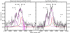 |
Fig. 3. Observed and synthetic spectra of J0929+0333. The abscissa corresponds to the rest frame wavelength in Å; the ordinate is the flux normalized to the continuum at 1350 Å. Left: black line: observed spectra minus the continuum; pink: model fit using specfit. The BC emission of AlIII and SiIII] are shown in purple, CIII] emission is shown in red, and the Fe III template is shown in green. Right: black line: the synthetic spectrum composed of the sum of the emission line components plus noise. The BC emission of AlIII (the sum of the doublet) and SiIII] are again shown in purple, the CIII] emission and the Fe III template are shown in red and green, respectively. |
Although our sample is composed of objects from the same population, we still expect some spectral diversity, most spectra differ in S/N and fitted components (e.g., BLUE AlIII, Fe IIIλ1914). Therefore we chose a set of characteristic spectra for the 1900 Å region and another set for the 1550 Å and 1400 Å region.
For the 1900 Å region we chose 7 models from the spectra J1259+0752, J0020+0740, J1419+0749, J2145−0758, J1231+0726, J1618+0705 and J0107−0855, with EWs of 11, 23, 15, 20, 19, 11 and 17 Å respectively (the input parameters for these models are described in Tables 2 and 3). Taking as an example the error models derived from J0020+0740, for the S/N = 50 model the routine estimated an error of ∼20% for the flux and ∼25% for the FWHM, as we decrease the S/N the error percentage increases, so for the S/N = 10 model the routine estimated an error of ∼40% for the flux and ∼45% for the FWHM. So for spectrum with a high S/N the associated error will be lower than those with a lower S/N, this behavior is shown in all of our error models and is in agreement with our measurement’s main source of uncertainty.
Measurements in the 1900 Å blend region.
Additional measurements in the λ1900 region.
Since the 1400 Å and 1500 Å region are similar in components and shape, the same uncertainties obtained for the C IV line has been used also for the 1400 SiIV + OIV] blend. For these regions we chose 5 models from the spectra J0847+0943, J0929+0333, J1214+0242, J1231+0725 and J1259+0752 with EWs of 9, 14, 9, 21 and 3 Å respectively (the input parameters for these models are described in Table 4).
Measurements in the λ1550 region.
The random models are generated with our routine, which consists of five basic steps:
1. Create an array of possible values for each free parameter, where the free parameters are:
– intensity of the emission line −50/+250% in steps of 1% from the original amplitude.
– centroid position within ±10 Å for symmetric unblended emissions, and ±2 for heavily blended BC lines (e.g., SiIII]λ1892, CIII]λ1909). For asymmetric emissions we used an asymmetric range of variation −15/+2 Å to avoid contamination from the BLUE component to the BC one. All variations were carry out in steps of 0.1 Å.
– FWHM: we vary the width of the emission −50/+250% in steps of 1 km s−1.
2. Create a model, using our routine, with random parameters from our arrays.
3. Iterate the routine; we decided to settled for 1 000 000 iterations which translates into 1 000 000 random models. The random iterations yield a distribution of values for line fluxes.
4. Prune the distribution so that only cases with χ2 consistent within a 2σ confidence level from the minimum χ2.
5. Compute the dispersion of the distribution for each model with given W and S/N. The dispersion is the uncertainty at 1σ confidence level.
The routine identifies the best fit minimizing the reduced  defined as:
where fo is an element of the random model array, fe is an element of the given input, σ2 is the quadratic spread of the random model with the original signal, and nd is the number of degrees of freedom. The summation runs up to n, the length of the arrays which match the length of the array for the input spectra (i.e., the analyzed spectral region resampled to 1 Å).
3.5. Measurements of profile normalized intensities
The specfit multi-components fits are time-consuming procedures. In order to compare specfit results with a simpler procedure we measure the intensity in specific radial velocity ranges of the emission lines to be used as metallicity indicators.
We create a routine using Python which yields the amplitude in the region given an input central wavelength and around it ±1000 km s−1. The first range is centered at 0 km s−1 and corresponds to the wavelengths where the BC emission is dominating (red dashed lines in Fig. 4). To represent the BLUE component with any actual profile decomposition, we measure the line intensity on the profile at −4000 km s−1 from the broad component (blue dashed lines in Fig. 4) and ±1000 km s−1 around this wavelength (gray area in Fig. 4). We chose the BLUE component position carefully with an offset with respect to the rest frame in order to avoid absorptions and to sample a spectral range where we expect emission from outflowing gas. In the case of an absorption line within the range of our measurement this results in negative values, which are not physical meaningful and therefore were ignored. To estimate errors we measured the distribution of the amplitudes within ±1000 km s−1 for each central wavelength component (grey areas in Fig. 4).
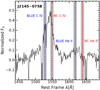 |
Fig. 4. Example of the 1550 Å region used for profile ratio measurements. The Figure shows in black the observed spectra minus the continuum. The red dashed lines indicate the rest frame wavelength of CIV and He II, the gray area surrounding these lines show the ±1000 km s−1 range of intensity measurement. The blue dashed lines indicate the BLUE emissions and are −4000 km s−1 from their broad component companion, the gray area surrounding these lines also show the ±1000 km s−1 range of measurement. Abscissa correspond to the rest frame wavelength in Å and ordinate normalized flux. |
Even though the BC CIV is the main emission of the 1550 Å region, Fig. 4 shows that the peak of maximum intensity is on the blue side of the region despite of the Mg IIλ2800 redshift correction. This behavior is present in the majority of the sample which lead as to believe that the BLUE emissions are a constant in the process in xA sources instead of a occasionally emission.
3.6. Estimation of physical parameters: MBH, luminosity, L/LEdd
We determined some basic physical parameters using the continuum splot measurements such as the bolometric luminosity (Lbol), the central supermassive black hole mass (MBH), and the Eddington ratio (L/LEdd); in addition, we computed the virial luminosity (Lvir). The estimated parameter values are presented in Sect. 4.3, and details of the computations are reported below.
Bolometric luminosity. We used the conventional way to derive the luminosity,  where dc is the comoving distance according to Sulentic et al. (2006)
![$$ \begin{aligned} d_\mathrm{c} \approx \frac{c}{H_0}\left[ 1.500(1-e^{-\frac{z}{6.309}}) + 0.996(1-e^{-\frac{z}{1.266}})\right], \end{aligned} $$](/articles/aa/full_html/2022/11/aa42837-21/aa42837-21-eq6.gif)
and c is the speed of light, H0 the Hubble constant assumed as 70 km s−1 Mpc−1 and z the source final redshift that is, the SDSS redshift after correction. The flux f = λfλ is in the quasar rest frame. A bolometric correction factor according to Richards et al. (2006) was applied to compute the bolometric luminosity.
Black hole mass and Eddington ratio. Black hole mass estimations tend to be over-estimated when using C IV-based scaling relations because of its strong blue excess (Marziani et al. 2019). In an effort to obtain a more accurate estimation we used the AlIII-based mass scaling relation proposed by Marziani et al. (2022):
![$$ \begin{aligned}&\log {M_\mathrm{BH} }(\mathrm {Al\ III} ) \approx (0.579^{+0.031}_{-0.029})\log L_{1700,44} \nonumber \\&\qquad \qquad \qquad \quad + 2\log [FWHM \mathrm {(Al\ III)} ] + (0.490 ^{+0.110}_{-0.060}). \end{aligned} $$](/articles/aa/full_html/2022/11/aa42837-21/aa42837-21-eq7.gif)
This relation requires only two parameters L1700, 44 the continuum luminosity at 1700 Å normalized by 1044 erg s−1 and the FWHM of AlIII in units of km s−1.
Using the MBH obtained from the previous step we estimated the Eddington luminosity following
Given this luminosity we obtained the Eddington ratio (L/LEdd), which is an indicator of the BH accretion rate.
Virial luminosity. We computed the redshift-independent virial luminosity in the form proposed by MS14:
where the ℷ is a function of the AGN SED and of the Eddington ratio that can be assumed constant and equal to 1 for the xA population. The product nHU has been normalized to the typical value 109.6 cm−3 and δν to 1000 km s−1 (more details are provided by Negrete et al. 2018; Dultzin et al. 2020). In practice, the virial luminosity has been computed by multiplying the numerical factor and the virial estimator δv (FWHM AlIII), raised to the fourth power.
3.7. Photoionization modeling
To interpret our fitting results we compare the line intensity ratios for BC and BLUE observed components with the ones predicted by CLOUDY simulations (Ferland et al. 2017). An array of simulations is used as reference for comparison with the observed line intensity ratios. It was computed under the assumption that (1) the column density is Nc = 1023 cm−2; (2) the continuum is represented by the model continuum of Mathews & Ferland (1987) which is believed to be appropriate for Population A quasars, and (3) the microturbulence is negligible. The simulation arrays cover the hydrogen density range 7.00 ≤ log(nH)≤14.00 and the ionization parameter −4.5 ≤ log(U)≤1.00, each in intervals of 0.25 dex. They are repeated for values of metallicities in a range encompassing five orders of magnitude: 0.01, 0.1, 1, 2, 5, 10, 20, 50, 100, 200, 500 and 1000 Z⊙. Extremely high metallicity Z ≳ 100 Z⊙ are considered to be physically unrealistic (Z ≈ 100 Z⊙ implies that more than half of the gas mass is made up by metals!), unless the enrichment is provided in situ within the disk, a possibility briefly discussed in Sect. 5.5. In several cases, simulations suffered convergence problems if Z ≳ 500 Z⊙. The behavior of diagnostic line ratios as a function of U and nH for selected values of Z are shown in the Appendices of S21.
4. Results
We aim to estimate the metallicity (Z) of the xA sources, as well as the correlations between Z and physical parameters. We first report the measurements of the emission line components, and of their ratios (Sect. 4.1), and then consider the results of Z estimates. After confirming the xA nature for most sources of our sample (Sect. 4.2), we seek for correlations in the sample (Sect. 4.3). Thereafter we present the Z estimates, first assuming fixed physical conditions (i.e., for a given nH and U, different for the regions associated with BLUE and BC, Sect. 4.4), and then considering nH and U free to vary (Sect. 4.4.2). We discuss the spectral appearance of a few subgroups and of some remarkable objects in the sample in Appendix B.
4.1. Immediate results
The analysis of the spectra involve the de-blending of broad and BLUE components. The rest-frame spectra with the continuum placements, and the fits to the blends of the spectra are shown in Appendix A. We isolate the contribution of the components in two ways: (1) using the specfit task, and (2) measuring the amplitude of the emission ±1000 km s−1 around a central wavelength.
4.1.1. Specfit measurements.
Tables 2 and 3 report the measurements of the 1900 Å region. The columns in Table 2 list (1) SDSS identification short code, (2) equivalent width between 1780–2000 Å, (3) the FWHM of AlIII and SiIII], (4,5) AlIII and SiIII] line fluxes, (6,7) CIII] FWHM and flux and (8,9) the measurements of the emission of iron at 1914 Å. Table 3 reports the additional measurements for the presence of an excess of AlIII for six sources. The Columns list (1) the SDSS identification short code, (2,3) the FWHM and flux, (4) the separation of the peak of the BLUE component from the rest-frame wavelength of AlIII in units of angstroms, and (5) the asymmetry (the skewness parameter as reported by specfit) of the emission line. Table 4 reports the measurements of the 1500 Å region for both BLUE and BC components. The columns list (1) the SDSS identification short code, (2) the equivalent width between 1450–1680 Å, (3) broad components’ FWHM, (4,5) flux of CIV and He II BC, (6) BLUE components’ FWHM, (7,8) flux of CIV and He II BLUE, (9) the separation of the peak of the BLUE component from the rest-frame wavelength of CIVλ1549BC in units of Å and (10) the asymmetry of the BLUE component according to specfit. Lastly, Table 5 lists the results for the 1400 Å region for both BLUE and BC components in the following order: (1) SDSS identification short code, (2) equivalent width between 1340–1450 Å, (3) broad component FWHM, (4) flux of SiIVBC, (5) BLUE component FWHM, (6) flux of SiIV+OIV] BLUE, (7) the separation of the peak of the BLUE component from the rest-frame wavelength of SiIV BC in units of Å, and (8) the asymmetry of the emission line. Table 6 reports the flux ratios of the metallicity indicators that will be used to estimate the metal content alongside CLOUDY simulations.
Measurements in the λ1400 region.
specfit Flux ratios dependent on metallicity.
4.1.2. Normalized intensities measurements.
Table 7 reports the measurements of the three regions. For the CIV and SiIV regions, measurements are reported for two ranges, one corresponding to the rest frame and a second meant to measure the blue-shifted excess. The columns list SDSS identification short code and the normalized intensities. Table 8 reports the ratios of the metallicity indicators.
Normalized intensities.
Flux ratios dependent on metallicity of normalized intensities measurements.
4.1.1. BC intensity ratios
Figure 5 includes the individual ratios that are used to distinguish xA sources. The lower panels show the results for individual non-BAL QSOs and their errors. The vertical continuous lines show the mean values of the distributions and the dashed vertical lines are set to 1 for SiIII]/He II and CIII]/He II. For AlIII/SiIII] and CIII]/SiIII], the dashed vertical lines are set to 1 and 0.5 respectively according to xA criteria. The outlying sources identified were J0103−1104, a low EW source with a strong CIII] emission, and J1231+0725, a BC-dominated spectrum with a faint BLUE.
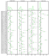 |
Fig. 5. Distribution (top) and individual (bottom) values of intensity ratios between prominent lines not used to estimate metallicity. The two panels on the right (AlIII/SiIII] and CIII]/SiIII]) show the ratios involved in the identification of xA sources. Vertical solid lines identify the mean value of the distribution. Dashed lines are set to 1 for the SiIII]/He II and CIII]/He II distributions, and 0.5 and 1.0 for the AlIII/SiIII] and CIII]/SiIII] distributions respectively, according to the UV selection criteria for the xA (Sect. 4.2). |
The left panel of Fig. 6 shows the normalized distributions of the diagnostic intensity ratios AlIII/He II, CIV/He II and SiIV/He II for the BC, while the right panel shows the diagnostic intensity ratios of CIV/AlIII, SiIV/CIV and SiIV/AlIII broad components. The vertical lines identify the mean values of the distributions: μ(AlIII/He II) = 3.70, μ(C IV/He II) = 5.42, μ(SiIV/He II) = 5.55, μ(C IV/AlIII) = 1.86, μ(SiIV/CIV) = 1.01 and μ(SiIV/AlIII) = 1.78.
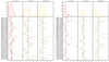 |
Fig. 6. Distribution (top) and individual (bottom) values of intensity ratios of the broad components used as diagnostics for Z involving HeIIλ1640 (left), and not involving HeIIλ1640 (right). Values are reported in Cols. 2 to 7 of Table 8. |
The distribution of the data points involving He II (Fig. 6 left panel) shows a small dispersion from the sample mean with the exception of J1609+0654, a type-1 QSO with weak broad components especially for He II which for this case was more likely underestimated due to absorptions and low S/N. Figure 6 right panel distributions shows more sources outside the trend. An example is J1231+0725, a clear non-xA source. Higher values of the CIV/He II and SiIV/He II ratios are associated with higher ionization parameters and with the 3 cases of non-xA and borderline sources identified in Sect. 4.2.
Since the three He II ratios are, for fixed physical conditions, proportional to metallicity, we expect an overall consistency in their behavior i.e., if the ratio for one object is higher than the sample mean, the other intensity ratios for the same object should also be higher. The lower panels are helpful to identify sources for which only one intensity ratio deviates significantly from the rest of the sample. The lack of consistency in the distributions of line ratios not involving HeIIλ1640 shown in the right panel of Fig. 6 was also found for its CLOUDY metallicity relations for fixed physical conditions (see Sect. 5.2). Hence, these relations will not be considered for further analysis.
4.1.2. BLUE intensity ratios
Figure 7 shows the distributions of the diagnostic intensity ratios between the BLUE components of C IV/He II, (SiIV + OIV])/He II and C IV/(SiIV + OIV]). The vertical lines identify the mean values of the distributions, μ(CIV/He II) = 5.17, μ((SiIV + OIV])/He II) = 2.11, μ(C IV/(SiIV + OIV])) = 2.64. The distributions show wide error bars as well as large dispersions. For most of the sources, the SiIV + OIV] BLUE component emission is slightly weaker than CIV BLUE component, resulting in well-behaved distributions with the exception of J2116+0441 and J2145−0758 that show weak SiIV + OIV] BLUE emission surrounded by absorptions and affected by poor S/N. BLUE CIV/(SiIV + OIV]) ratios show an apparently more confused distribution. However, two groups can be identified: a majority one with median BLUE C IV/(SiIV + OIV] ≈ 2.5, and a minority one with larger BLUE CIV/(SiIV + OIV]) ≈ 4. The higher ratios that can be linked to heavy absorptions affect the SiIV + OIV] profile. The source J1215+0326 shows the highest ratio due to the strong absorption in both wings of the 1400 Å region. Indeed the BLUE ratios for J1215+0326 appear not to be fully consistent due to the absorption that affects also the red side of the SiIV profile and introduces a large source of uncertainty.
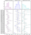 |
Fig. 7. Intensity ratios for the BLUE components, shown in the same layout of the previous figures. Values are reported in Cols. 8 to 10 of Table 8. |
4.2. Identification of xA sources and of “intruders”
Figure 8 shows the UV-plane selection criteria. The vast majority of our sample are xA quasars except for the two sources, J0103−1104 and J1231+0726 that were previously identified as outlying sources. They show a spectra not consistent with the xA spectral type and will not be considered for further statistic analysis. On the converse, the borderline object J0946−0124 is outside the xA part of the parameter plane. However, its error bars indicate that the criteria are still satisfied within 1σ confidence level. The overall appearance of the spectrum (Fig. A.1) supports the classification of J0946−0124 as an xA source.
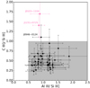 |
Fig. 8. Relation between AlIIIλ1860/SiIII]λ1892 and CIII]λ1909/SiIII]λ1892 intensity ratios. The gray area corresponds to the parameter space occupied by xA objects. Outlying sources are shown in pink color. |
The lack of a clear trend shown in Fig. 8 may be due to the prior selection criteria for the xA bin in the 4DE1 parameter, because we are zooming into one bin of the 4DE1 that shows a small dispersion around well-defined parameter values.
4.3. Correlation between diagnostic ratios and physical parameters
Table 9 reports the physical parameters estimations, including the 6 BAL QSOs. The columns list (1) SDSS identification short code, (2) logarithm of the supermassive black hole mass in solar masses, (3),(4) the bolometric luminosity and virial luminosity in units of erg/s and (5) the Eddington ratio. Figure 9 shows the correlations between all diagnostic ratios employed in this work. Blue plots (left lower matrix) show the correlations between the diagnostic ratios from Table 6, for both broad and blue components. Green plots (upper right matrix) represent the correlations between the physical parameters derived for each object. The pink dots correspond to the intruders described in Sect. 4.2 and are not considered for the statistic analysis. In order to get a better correlation we also excluded from the analysis sources located very far from the main relation in the parameter plane due to measurement problems, the most frequent ones being absorptions and low S/N. These sources are shown as black dots. The solid lines show the linear relation for the remaining sources. The Spearman correlation coefficient is reported at the top right corner of each panel.
Physical parameters.
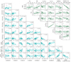 |
Fig. 9. Correlations between diagnostic ratios for the broad and BLUE components (left lower matrix), and between physical parameters (right upper matrix). The pink dots are the outlier sources described in Sect. 4.2 and were not considered in the statistical analysis. Additionally, for each panel we excluded, if necessary, the objects with the highest dispersion from the main relation (black dots). The blue and green dots are the values considered for each relation, the solid lines show the linear fit, the shaded areas represent the confidence interval of the lineal regression. For each relation the Spearman correlation coefficient (r) is shown in the right top corner. |
Most of the relations in Fig. 9 show a weak trend, in spite of the elimination of outlying sources. This may be due to the prior selection criteria for the xA bin in the 4DE1 parameter, because we are zooming into one bin of the 4DE1 that shows a small dispersion around well-defined parameter values.
The panels involving BLUE CIV/(SiIV + OIV]) (second row from bottom) show no significant correlation as the flux ratio remains approximately constant. This constant value may imply that the wind emission in the HILs is active throughout the sample, and that the emitting gas might be in similar physical conditions.
The relations that show the highest correlation coefficient (r > 0.77, last two panels of the last row) are between the BLUE components. However, these ratios are not statistically independent since they involve the same lines in abscissa and ordinate, and all of them are HILs and need similar conditions to occur.
Among all the ratios in the correlation matrix the most significant result is the relation between BLUE CIV/He II and BC CIV/AlIII with a correlation coefficient of r = 0.626, showing a connection between the metallicity indicators for the BC and the BLUE. This correlation is consistent with the overall high-Z scenario emerging from the present work: BLUE C IV/He II decreases with increasing CIV/AlIII, and both ratios increase with decreasing metallicity (Sect. 5.2 and following). However, also this anticorrelation should be viewed with care: most of the data points cluster around a typical value.
4.4. Metallicity inferences
As mentioned in Sect. 3.7, we use flux ratios as metallicy diagnostics for the BLR gas. The foundations of the method we apply are explained in S21. Here we briefly recall two main aspects.
Among all the indicators proposed by different authors (e.g. Nagao et al. 2006b; Shin et al. 2013; Marziani & Sulentic 2014) we give higher weight to the indicators involving HeIIλ1640. The diagnostics ratios are AlIII/HeIIλ1640, CIV/HeIIλ1640, and SiIV + OIV]/HeIIλ1640 for the virialized BC, and CIV/HeIIλ1640, SiIV + OIV]/HeIIλ1640, CIV/HeIIλ1640, and SiIV + OIV]/CIV for BLUE. We also considered the fitting complex for regions with λ < 1300 Å. However, even though NIV]λ1486 is present for most of our sample, we decided to avoid its fitting procedure because it appears to be weak, and in some cases it is severely affected by absorptions.
We modeled the BLR assuming gas in much different physical conditions for the virialized and for the wind component:
– Virialized: assumed with log(nH) = 12–13 and log(U)= −2.5;
– Wind: assumed with log(nH) = 9 and log(U) = 0.
The assumptions on the density and ionization parameter for the virialized component stem from several studies suggesting low-ionization and high density (Baldwin et al. 1996, 2004; Marziani et al. 2010). Further work has set robust lower limit to the density of the low-ionization region, from the strength of IR CaII triplet and of the Fe II emission blend (Matsuoka et al. 2007; Martínez-Aldama et al. 2015; Panda et al. 2018, 2020b,a) at log nH ≈ 11.5. The low C IV/Hβ ratios for the virialized component is best explained by a modest ionization parameter, log U ∼ 2.5 (Marziani et al. 2010; Panda et al. 2020b). These values are in agreement with the most recent determination of Śniegowska et al. (2021). The blueshifted component is by far less constrained. The higher C IV/Hβ suggests higher ionization parameter than for the virialized component (Marziani et al. 2010; Śniegowska et al. 2021). The absence of a strong blueshifted component in AlIII indicates moderate density, likely around log nH ∼ 10. For this density the lack of any obvious CIII] blueshifted component (detection that may be however hampered by the severe blending with SiIII]) implies very high ionization parameter log U ∼ −0.5 − 0.
4.4.1. Estimates of Z distributions at fixed (U, nH)
Our six metallicity indicators are shown in Fig. 10. Left panel shows the low ionization zone metallicity indicators, and right panel shows the high ionization potential metallicity indicators or BLUE component indicators. For both panels the stars represent the flux ratios predicted by CLOUDY according to the specified physical conditions, we fit each CLOUDY trend with a cubic spline (dashed lines) and derive the metallicity of our sample according to it. The thicker solid lines show the ranges of metallicity derived from our sample.
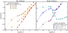 |
Fig. 10. Intensity ratios trends predicted by CLOUDY as a function of the logarithm of the metallicity, for fixed physical parameters U and nH. Left panel: ratios of low/intermediate ionization potential BC lines. Right panel: ratios for high ionization potential emissions (BLUE components). In both panels, the stars represent the ratios predicted by CLOUDY. The dashed lines are the interpolation between the CLOUDY values obtained with a cubic spline, the thick solid line segments in each trend line show the range of line ratios covered by our sample, according to the measured flux ratios. |
In order to seek for a better description of the BLR, we decided to use two cases of density log(nH) = 12 and log(nH) = 13 for the BC ratios but keeping the ionization parameter fixed at log(U) = −2.5. These high nH values are needed to explain Fe II and the UV emission lines in the virialized component, as briefly summatized above. Table 10 lists the derived metallicities for the three broad component metallicity indicators and their median value (Zμ1/2) for the log(nH) = 12 and the log(nH) = 13 case. Left panel of Fig. 10 shows only the case for log(nH) = 12, it can be seen that our three BC indicators show a consistent trend. The derived median value is Z = 1.73 ± 0.15 Z⊙ for the virialized clouds as reported in Table 10. The errors for the metallicity estimates, both BC and BLUE relations, were estimated following the flux ratio error propagation but considering them as relative errors for their logarithmic display.
Metallicity (log Z) of the BC assuming fixed U, nH.
The wind clouds were described with a density of log(nH) = 9 and a ionization parameter of log(U) = 0, as shown in the right panel of Fig. 10. These ratios do not show consistent relations, especially for the BLUE CIV/He II ratio with a nonmonotonic trend (also shown in Fig. 17 of S21). The non-monotonic behavior occur in the interval from subsolar to super solar metallicity, which means that one value of the BLUE CIV/He II ratio may correspond to three values of the metallicity. Thus, for the sources that cross the trend (blue dashed line in Fig. 10) in three points we decided to take the average value. Table 11 lists the derived metallicities for our three BLUE metallicity indicators and their median value, with a general median value of Z = 0.77 ± 0.13 Z⊙ (as reported in Table 11), setting a lower metallicity limit for our sample.
Metallicity (log Z) of BLUE assuming fixed U, nH.
Figure 11 left panel shows the metallicity estimates distributions in log(Z/Z⊙) for the BC intensity ratios shown in Fig. 6. The right top and bottom panels show the superimposed estimates from the three ratios and their median values in black. The values derived from the BC CIV/He II relation are the ones with higher dispersion from the general median especially those with a strong He II feature such as J0034−0326 (Fig. A.1) and J0903+0708 (Fig. A.1).
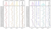 |
Fig. 11. Distribution (top panels) and individual (bottom panels) values of line ratio metallicity estimate involving HeIIλ1640 using broad components (left) and BLUE components (right). |
Figure 11 right panel show the metallicity estimates distributions in log(Z/Z⊙) for the BLUE intensity ratios shown in Fig. 7. The right top and bottom panels show the superimposed estimates from the three ratios and their median values in black. What stands out the most is the bivaluated behavior of the BLUE CIV/He II estimates, this is caused by the non-monotonic behavior of the respective CLOUDY relation shown in Fig. 10. For the sources crossing the trend in three points, the dots are the mean of the three possible values and the error bars are extended to lowest point where the source cross the trend (negative error bar) and the highest point where the source cross the trend (positive error bar).
4.4.2. Estimates of Z relaxing the constraints on U and nH
Table 12 reports the results of the analysis relaxing the assumptions of fixed values of nH, U. We used the complete range values of hydrogen density 7.00 ≤ log(nH)≤14.00 and the ionization parameter −4.5 ≤ log(U)≤1.00 described in Sect. 3.7. The log Z, log U, log nH and their associated uncertainties are reported for 33 sources of the sample (excluding BAL QSOs, and sources that are not xA). The exclusion of sources that are not xA is due to the fact that their SED may not be consistent with the ones of the Population A sources: even if the intensity ratio can be measured with good precision, the present set of CLOUDY simulation cannot be used to predict the metallicity of these sources. The last two rows list the results for the median computed from the median of the ratios of the individual sources,  (Ratios), and the one computed from the medians of the individual object parameter values,
  (Objects). The parameters reported in Table 12 and shown in Fig. 12 cluster around well-defined values, with medians ≈50 Z⊙, ionization parameter log U ≈ −2, and very high density log nH ≈ 13.75. These values are in good agreement with S21, implying that the additional sources that are now the majority of the sample and meet the selection criteria for being xA, also show ionization degrees and metallicity values in the same range. The result is largely a consequence of the inclusion of AlIII in the diagnostics. This line, involved also in the selection criteria, is very strong in xA with respect to quasars belonging to other spectral types along the main sequence (Aoki & Yoshida 1999; Bachev et al. 2004), and AlIII strength is favored at high Z, high nH.
Z, U and nH of individual sources and median derived from the BC.
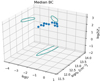 |
Fig. 12. Parameter space nH, U, Z. Data points in 3D space are elements in the grid of the parameter space selected for not being different from |

Two groups of sources stand out. The first one includes (1) sources that are extreme with Z ∼ 100 Z⊙. These sources have a large fraction of their gas mass made of metals (S21); (2) sources with relatively high U ∼ −1.5. Five out of seven sources of the 1st group show the highest SiIV compared to CIV and are at the low end of the distribution of CIV and AlIII equivalent widths. However, J2116+0441 and J2145-0758 show relatively prominent CIV and lower SiIV, probably as an effect of a higher ionization parameter. The second group has higher CIV/AlIII than average, although this has no strong implication for Z: if log U ∼ −1.75, the median log Z ∼ 1.7 [Z⊙]; only in two cases with log U ∼ −1.5, the median log Z ∼ 1.3 [Z⊙], lower than the full sample median.
Table 13 provides the information on metallicity that is possible to extract from the BLUE intensity ratio. No nH and U values are reported, as they are very poorly constrained (Fig. 13). The bottom panel shows the median case reported in Table 13 and reveals the existence of two main emitting regions in the parameter plane U vs. Z. The range reported in Table 13 is the Z range possible for the high-ionization and the intermediate ionization range (U ∼ −2, right panel of Fig. 13).
Z, U, nH of individual sources and median derived from BLUE.
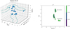 |
Fig. 13. Left: parameter space nH, U, Z, as in Fig. 12, but for component BLUE. As in that case, data points were computed from the emission line ratios referring to the median values in Table 6. The individual contour line was smoothed with a Gaussian kernel. Right: the plane log U vs. log Z. The outer isophotal contours delimit the region χmin + 1, where the χmin is the value after smoothing with a Gaussian filter. The low- and high-ionization solutions are marked. |
5. Discussion
We focus the discussion on three main topics: (1) the adequacy of the fitting methods, comparing the specfit and the profile ratios as well as the results on diagnostic ratios and Z obtained in this paper and the ones of S21; (2) the correlation between Z and relevant physical and observational parameters. Of them, the CIV integrated properties appear to be especially relevant; (3) the possibility of elemental pollution i.e., that the relative abundances of the elements deviate from the ones of solar chemical composition.
5.1. Fitting methods
5.1.1. specfit vs. profile ratios
Figure 14 compares the measurements of our six metallicity indicators for the two methods employee in this work, the specfit analysis (Sect. 3.3) and the ratios of profile normalized intensities (Sect. 3.5). Each panel shows the equality line (black solid line) and the errors bars according to the fitting method. Top panels correspond to the BC ratios and bottom panels to the BLUE ratios. The identified black dots are sources that stray out from the rest of the sample, the cause of this behavior is different for BC and BLUE ratios:
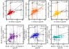 |
Fig. 14. Top, from left to right: relation between intensity ratios CIV/HeIIλ1640, AlIII/HeIIλ1640 and CIV/HeIIλ1640 BC computed with specfit and with profile ratio technique described in Sect. 5.1.1. Bottom: comparison of intensity ratios for (SiIV + OIV]])/HeIIλ1640 for the BLUE component. Sources with the largest discrepancy from the equality line are identified. |
– BC ratios black dots (e.g. J0123+0329, J1545+0156, J1609+0654): this is due to deficient measurements of the He II emission which tend to be underestimated beside the CIV feature. The specfit modeling can compensate the surrounding narrow or broad absorptions while the profile measurements take the median intensity over a selected range directly from the spectra and can return close to zero or negative results for low S/N spectra.
– BLUE ratios black dots (e.g J1231+0725, J0034−0326, J2145−0758): what causes the discrepancies for the BLUE ratios is the strong absorptions in these three features. Similar to the discussed for BC ratios, the specfit modeling can compensates the missing information from the original signal while the profile measurements only takes the median of the existence intensity within a given range and for the case of absorptions the resulting median intensity is diminished, as briefly explained in Sect. 3.5, compare to the specfit measurements. We could modify the routine to skip the negative intensities (for the case of strong absorptions) but for profiles with less intense absorptions the result will still be the same.
The two measurements agree within the uncertainties in the wide majority of cases, being the BLUE CIV/(SiIV + OIV]) ratio the one showing the lower degree of correlation with a trend mainly constant. As reference we consider r≳0.4 as a lower limit for statistical significant correlation (with ≲ 1% of probability of not being correlated) for our ∼36 sources data set. If the BC CIV/He II ratios are compared, disagreements occur in the sense that the CIV/He II ratio measured with specfit is much lower than the one from the profile ratio. This is due to the fact that the specfit modeling compensates for narrow or broad absoprtion and is probably less affected by low S/N. The reverse case J1609+0654 is associated with absorption and low S/N at the He II rest frame that effects both the specfit results and the profile ratios. Similar considerations apply to the BLUE radial velocity domain: the outlier J1026+0114 is affected by an absorption that is interpolated across in the specfit model.
The comparison between the two methods of measurements show that, even in the fairly homogeneous sample of the present work, there is a range of values in the Z-sensitive diagnostic ratios: 2≲ CIV/HeIIλ1640 ≲10, 1≲ AlIII/HeIIλ1640 ≲6, 3≲ CIV/HeIIλ1640 BLUE ≲10. Outside of these range, extraordinarily large or small values are more likely due to measurement issues than to physical differences.
5.1.2. Comparison with the results of Śniegowska et al. (2021)
The agreement between the measurements in the present thesis and the ones in common with S21 is fair for a 13 sources data set, as shown in Fig. 15. For this subsample we are considering r ≳ 0.7 as a lower limit for statistical significant correlation (with ≲1% of probability of not being correlated). The main reason for this difference is most likely to a subestimation of the He II intensity in S21, yielding unrealistic values for the ratios involving He II. The difference between the medians for the two sets of measurements for the ratio CIV/HeIIλ1640 BC is ≈0.05 ± 0.11 dex, i.e., within the observational uncertainty. The source that is deviating most in Fig. 15, J0858+0152 is associated with the difficult continuum placement around 1640 Å: the value of HeIIλ1640 intensity reported by S21 is most likely an underestimate. The discrepancy brings attention to the need to consider high S/N for the measurement of the HeIIλ1640 line. However, the measurements remain statistically consistent with a median deviation of ≈ − 0.04 ± 0.12 for AlIII/HeIIλ1640. The BLUE CIV/HeIIλ1640 ratio measurements appear to be fully consistent (μ ≈ −0.02 ± 0.04 dex).
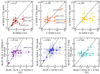 |
Fig. 15. From left to right: relation between intensity ratios CIV/HeIIλ1640, AlIII/HeIIλ1640, CIV/HeIIλ1640 BLUE, (SiIV + OIV]/)HeIIλ1640, and (SiIV + OIV]/)HeIIλ1640 BLUE for the 13 objects in common with S21. The labels identify sources with largest deviation from the 1:1 lines. |
The derived Z values from the CIV/HeIIλ1640 BC for fixed physical conditions are also in very good agreement: the median difference for the 13 objects in common is ≈0.11 ± 0.22, with the SIQR scatter less than a factor ≈2, correspondent to the uncertainties associated with the method.
Regarding the BLUE component, a comparison is possible only for eight objects. The free log Z estimates are ≈1.3 and 1.0 for S21 and the present work, suggesting metallicities typically in between 10 and 20 times the solar value.
5.2. Analysis of Z distributions at fixed (U, nH) for specfit and profile ratio measurements
Table 14 lists the Z results for the normalized profile measurements, and we compare the metallicity results obtained with our two fitting methods in Fig. 16. The three upper panels showing the comparison for AlIII/He II, CIV/He II, SiIV/HeIIλ1640 demonstrate a high degree of correlation between the two methods, with the slope of the best fitting line close to the 1:1 relation. For the BLUE component, the situation is less clear. The CIV/(SiIV + OIV]) ratio is basically a scatter-plot: all sources are apparently with typical metallicities in the range log Z/Z⊙ ∼ 0.6 − 1.1. Some of our sources show a low S/N mainly around the 1400 Å and 1550 Å regions. This affects our measurements and metallicity estimates giving a ratio that can not find a solution with the CLOUDY metallicity relations. The case of CIV/HeIIλ1640 is especially cumbersome: due to the non-linear relation between ratio and Z, for some of the sources the two methods produce highly discordant values.
Metallicity of normalized intensities measurements.
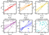 |
Fig. 16. Metallicity comparison of our two fitting methods. Abscissas corresponds to specfit results and the ordinates to profile ratio measurements results. Each panel shows the values per metallicity relation, top left corner indicates the Spearman correlation coefficient, the black solid line shows the equality line. Sources with the largest discrepancy from the equality line are discarded and identified as black dots. |
5.3. Correlation between Z and AGN physical properties
As we have previously mentioned in Sect. 4.3, due to the prior selection criteria for the xA bin and also to our narrow z range, we are not expecting clear trends between metallicity Z, luminosity, MBH and L/LEdd: we selected sources that are extreme in the 4DE1 parameter space. Instead, most of the results are yielding well-defined parameters that corroborate the efficiency of the 4DE1 selection criteria. For instance, the metallicity and the Eddington ratio are found not to be correlated (r ≈ −0.094; Fig. 9). Both parameters however show a small dispersion around well-defined values log(ZBC) = 1.73 ± 0.15 and L/LEdd = 1.01 ± 0.16. The lack of significant correlations can be seen in the upper right panels of Fig. 9. The only exception is the full profile of the CIV emission (BC + BLUE component) FWHM and centroid at half intensity (indicated as shift in Fig. 9): the Pearson correlation coefficient is r ≈ −0.97, and Spearman’s ≈ − 0.95. These values have extremely high significance for a sample of 36 objects. This result is however not immediately related to Z trends (the r values suggest no significant correlations of shift and FWHM of CIV with Z (see Fig. 9), and will be presented and discussed elsewhere.
5.4. Highly-supersolar abundances
Accepted at face value, the Z derived for the virialized component of the BC implies metallicities 20–50 times the solar values. These determinations are consistent with the results of S21 who also found median values of 50, 20, 80 for the Z estimated from the AlIII/He II, CIV/He II, SiIV/He II ratios, respectively. Similarly in both studies a median Z ≈ 50 Z⊙ is found if the condition of fixed nH and U is relaxed. The consistency with S21 is in a way hardly surprising, since the method of measurement and analysis is the same, and the quasars belong to the same spectral class.
Changes in metallicity that are associated to changes in the physical conditions (U, nH) for the BC are modest. A small change in the Z estimates are possible if the U is increased by ∼0.5 to 1 dex, up to log U ∼ −1.5. In this case, the median Z derived for our sample would decrease to log Z/Z⊙ ≈ 1.2. Increase of nH or decrease in U would increase the Z estimates. The last 3 columns of Table 10 report the values if the density is increased to nH = 1013 cm−3: in this case the values remain very high ∼100 Z⊙, and the difference between the estimation from CIV and AlIII is reduced. The parameter space (nH, U, Z) shown in Fig. 12 indicates that the Z is well-constrained, and that a change in physical conditions still satisfying the observed ratios would imply a change in Z, i.e. δlog Z ≲ 0.5.
The values we obtain for the BC are therefore consistent with Z ≳ 20Z⊙. This value should be taken as a reference for further discussion, and is not much higher from the estimate obtained for high-z quasars in several previous studies (Baldwin et al. 2003; Warner et al. 2004; Nagao et al. 2006a; Shin et al. 2013; Sulentic et al. 2014) that indicate Z ∼ 10 Z⊙ in sources that are not as extreme as the one considered here, with lower AlIII and SiIV with respect to CIV. These conditions can be interpreted as associated with lower Z.
The Z values derived for the BLR of quasars are instead very high in the context of their host galaxies: the highest Z value measured in molecular cloud is around 5 Z⊙ (Maiolino & Mannucci 2019). However, the nuclear and circumnuclear regions of quasars differ markedly from a normal interstellar environment. The passage of stars through the disk involves the formation of accretion modified object that eventually reach high mass and explode, after a short evolution, as core collapse supernovae (Collin & Zahn 1999; Cheng & Wang 1999). Stars in the nuclear region can rapidly become very massive (M ≳ 100 M⊙). These stars undergo core collapse, and contribute to polluting the disk with heavy elements through the high metal yields of supernova ejects (Cantiello et al. 2021). The compact remnants may continue accretion sweeping the accretion disk and giving rise to repeated supernova events (Lin 1997). The metallicity enhancement is predicted to lead to ∼10 − 20 Z⊙ (Wang et al. 2011), consistent with the value obtained for the xA sources.
5.5. Abundance pollution
This work xA sources were selected to have strong AlIII by definition, and the line is strongly sensitive to Z, for fixed physical condition. High nH and moderate or relatively high U contribute to make the line stronger (Marziani et al. 2020). Figure 17 shows the distribution of the metallicity differences δlog Z = log Z(AlIII) −log Z(CIV) and log Z(SiIV) −log Z(CIV). For the most likely values of the ionization parameter, −2 ≲ log U ≲ −2.5, the value of Z is consistently higher if derived from the AlIII/HeIIλ1640 ratio or SiIV/HeIIλ1640 ratio than from the one derived from CIV/HeIIλ1640, by a factor of ≈1.5 − 2. The very high Z values derived for the BC are due to the inclusion of the AlIII lines. While values ≈10 − 20 Z⊙ seems to be possible for the xA sources, higher values ∼50 − 100 Z⊙, might be more associated with deviation from the relative solar elemental abundances.
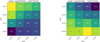 |
Fig. 17. Left panel: difference in the metallicity estimates from the AlIII/HeIIλ1640 intensity ratio and from the CIV/HeIIλ1640 ratio of the broad component, as a function of ionization parameter and density. The difference remain significant at a 2σ confidence level down to Δlog Z = log Z(AlIII/HeIIλ1640) − log Z(CIV/HeIIλ1640) ≈0.3. Right: same, for difference in the metallicity estimates from the (SiIV + OIV])/HeIIλ1640 ratio (≈SiIV/HeIIλ1640) and from the C IV/HeIIλ1640 ratio. The two cases with red values are lower limits. |
5.6. Metal segregation
The comparison between the Z derived from CIV BC fixed, and the Z for BLUE free can be carried out for both S21 and the present paper. The BC fixed medians are 1.7 (S21) and 1.3 (present paper), vs. 1.3 and 1.0 for the respective blue components. Considering that the uncertainty is δlog Z ≈ 0.3 dex, the comparison suggests an overall consistency in the Z determinations. However, in both works there is a small discrepancy between the Z estimates for the BC and BLUE. Selective enrichment of BLUE and BC is in principle possible. Radiation driven winds are primarily accelerated via resonant scattering of metal lines (e.g., Proga et al. 2000; Proga & Kallman 2004, Giustini & Proga 2019, and references therein). However, the metal ions are coupled to hydrogen and helium through Coulomb collisions, and physical conditions needed to lead a decoupling are extreme and outside the range considered for the BLR (Baskin & Laor 2012). A second mechanism is associated with the interaction of compact objects crossing the disk and the disk itself (Wang et al. 2011): star formation in self-gravitating disks can give rise to metallicity gradients in broad-line regions, with the higher Z in the innermost regions where a radiation driven wind is expected to develop. Also in this case, the wind component should be the more metal rich. The expected condition is that BLUE might be more affected by metal segregation (if at all), so that ZBLUE ≳ ZBC and not the converse, nor ZBLUE ∼ ZBC.
The very high Z estimates, reaching Z ∼ 100 Z⊙, are associated with the inclusion of the AlIII and SiIV lines. Z estimates from CIV/HeIIλ1640 may be consistent for BLUE and BC within the uncertainties, and suggest Z ∼ 10 Z⊙. Therefore, confirmatory data are needed for any discrepancy between BLUE and BC Z estimates, also considering that the diagnostics of the BLUE is poor. In addition to the difficulties in the measurement of the blue wings, the CIV/HeIIλ1640 has a nonmonotonic trend with Z at high U (as shown in the Appendix of S21). Our preliminary conclusion is that BLUE- and BC-derived Z values are consistent, if we exclude estimators that could be affected by elemental overabundance, as briefly discussed above.
6. Conclusion
We studied the UV spectroscopic properties of a sample of xA quasars focusing on their metal content. The sample sources are an extension of the sample of S21 which included only 13 objects, and was mainly aimed to assess the applicability of a method based on the intensity of the strong emission lines CIV, AlIII, SiIV + OIV] relative to HeIIλ1640, with the heuristic separation between a virialized (symmetric and unshifted, BC), and a blue-shifted component (BLUE).
The main result of the present investigation is the confirmation of very high metallicity values, in excess of 5 times solar, and more likely in the range 10–50 Z⊙, as found by S21.
– For the BC, and the most likely fixed physical condition (nH ∼ 1012 cm−3; U ∼ 10−2.5) suggest Z ≈ 50 Z⊙, with a 40% scatter. We remark that this high value is a consequence of the inclusion of the AlIII/HeIIλ1640 and SiIV + OIV]/HeIIλ1640 ratios in the Z estimate.
– For the BLUE, again at fixed physical conditions, the most likely value is Z ≈ 6 Z⊙. The discrepancy with the BC needs to be accounted for.
– Relaxing the assumption of fixed physical conditions, the three indepenent ratios allow for an independent estimate of nH, U, and Z. The results on Z are consistent with the case for fixed physical conditions (Z ≈ 50 Z⊙), the ionization parameter is log U ∼ −2, and the derived nH is however significantly larger.
– Without fixed physical conditions, Z ∼ 10 Z⊙ is found for BLUE, with U and nH largely unconstrained.
– We noted that the Z derived from CIV/HeIIλ1640 (Z ≈ 30 Z⊙) is lower than the ones from AlIII and SiIV + OIV]/HeIIλ1640. We explored the ratios between AlIII/HeIIλ1640 and CIV/HeIIλ1640 derived Z as a function of nH and U, and found that the difference is preserved within factors 1.5–5 in the range −2.5 < log U < −1.5, and 12 ≲ log nH ≲13 (cm−3).
– We tentatively explained this result by abundance pollution, and suggest that the elemental abundances of the BLR gas might be significantly different from solar, especially for elements like Silicon and Aluminum. Our suggestion is supported by the models that attempts to account for the complexity of the active nucleus, that encompasses star forming regions and even accretion-modified stars. The conditions of the xA sample are most likely very different from the ones expected in a passively evolving, elliptical host.
– Considering only the CIV/HeIIλ1640 as a Z estimator, we are left in the uncomfortable situation that the relation between this ratio and Z is not monotonic at high U. This effect involves the highest U down to log U ∼ −1. Therefore we consider that the best estimator for solar-metallicity estimates is the BC CIV/HeIIλ1640 ratio, that yields values around Z ≈ 30 Z⊙ with a sample standard deviation of 0.15 dex, implying 20 Z⊙ ≲ Z ≲ 40 Z⊙.
– The main accretion parameters (MBH, L, L/LEdd) of the present sample cluster around a well defined value, with modest scatter comparable to the individual error of measurements. The spectral similarity also suggest that we are observing almost “clones” of the same AGN. The L/LEdd value ∼1 confirms that these sources are high radiators.
– The present sample shows that the CIV full profile parameters are highly correlated among themselves, as seen in previous studies. Especially striking is the correlation between FWHM and centroid at half maximum. Since all relevant parameters are constrained in a small range, we suggest that the correlation is mainly due to orientation effects.
– The specfit analysis requires a multicomponent decomposition that may not be strictly unique. It is actually a model imposed to the data on the basis of trends observed along the quasar main sequence. To test the validity of this model, we also considered a model independent measure, based on the profile ratios in fixed wavelength range, where BC and BLUE give the maximum emission, but otherwise without profile decomposition.
The profile ratio method is in principle applicable to large samples of quasars that are highly accreting. However, it relies heavily on the HeIIλ1640 emission line which is weak and with a very broad profile (as true also for the optical He IIλ4686 emission, Marziani & Sulentic 1993). Dedicated observations yielding high-S/N are needed to improve the precision of the Z estimates. This is not a standard refrain: the potential of the method exploiting the HeIIλ1640 profile measurements can be unleashed only with precise He IIλ1640 measurements.
Acknowledgments
DD and CAN acknowledge support form grant IN111422 PAPIIT UNAM. CAN acknowledges support from CONACyT project Paradigmas y Controversias de la Ciencia 2022-320020. M.S. and S.P. acknowledge the financial support from the Polish Funding Agency National Science Centre, project 2017/26/A/ST9/-00756 (MAESTRO 9). S.P. acknowledges partial financial support from the Conselho Nacional de Desenvolvimento Científico e Tecnológico (CNPq) Fellowship (164753/2020-6).
References
- Aoki, K., & Yoshida, M. 1999, in Quasars and Cosmology, eds. G. Ferland, & J. Baldwin, ASP Conf. Ser., 162, 385 [NASA ADS] [Google Scholar]
- Bachev, R., Marziani, P., Sulentic, J. W., et al. 2004, ApJ, 617, 171 [NASA ADS] [CrossRef] [Google Scholar]
- Baldwin, J. A., Ferland, G. J., Korista, K. T., et al. 1996, ApJ, 461, 664 [NASA ADS] [CrossRef] [Google Scholar]
- Baldwin, J. A., Hamann, F., Korista, K. T., et al. 2003, ApJ, 583, 649 [NASA ADS] [CrossRef] [Google Scholar]
- Baldwin, J. A., Ferland, G. J., Korista, K. T., Hamann, F., & LaCluyzé, A. 2004, ApJ, 615, 610 [NASA ADS] [CrossRef] [Google Scholar]
- Baskin, A., & Laor, A. 2012, MNRAS, 426, 1144 [NASA ADS] [CrossRef] [Google Scholar]
- Boroson, T. A. 2002, ApJ, 565, 78 [NASA ADS] [CrossRef] [Google Scholar]
- Boroson, T. A., & Green, R. F. 1992, ApJS, 80, 109 [Google Scholar]
- Bruhweiler, F., & Verner, E. 2008, ApJ, 675, 83 [NASA ADS] [CrossRef] [Google Scholar]
- Buendia-Rios, T., Negrete, C. A., Marziani, P., et al. 2022, A&A, accepted, [arXiv:2209.05526] [Google Scholar]
- Cantiello, M., Jermyn, A. S., & Lin, D. N. C. 2021, ApJ, 910, 94 [NASA ADS] [CrossRef] [Google Scholar]
- Cheng, K. S., & Wang, J.-M. 1999, ApJ, 521, 502 [NASA ADS] [CrossRef] [Google Scholar]
- Collin, S., & Zahn, J.-P. 1999, Ap&SS, 265, 501 [NASA ADS] [CrossRef] [Google Scholar]
- Diamond-Stanic, A. M., Fan, X., Brandt, W. N., et al. 2009, ApJ, 699, 782 [NASA ADS] [CrossRef] [Google Scholar]
- D’Onofrio, M., Marziani, P., & Chiosi, C. 2021, Front. Astron. Space Sci., 8, 157 [Google Scholar]
- Du, P., Wang, J.-M., Hu, C., et al. 2016, ApJ, 818, L14 [NASA ADS] [CrossRef] [Google Scholar]
- Dultzin, D., Marziani, P., de Diego, J. A., et al. 2020, Front. Astron. Space Sci., 6, 80 [NASA ADS] [CrossRef] [Google Scholar]
- Ferland, G. J., Chatzikos, M., Guzmán, F., et al. 2017, Rev. Mex. Astron. Astrofis, 53, 385 [Google Scholar]
- Giustini, M., & Proga, D. 2019, A&A, 630, A94 [NASA ADS] [CrossRef] [EDP Sciences] [Google Scholar]
- Hewett, P. C., & Wild, V. 2010, MNRAS, 405, 2302 [NASA ADS] [Google Scholar]
- Kriss, G. 1994, Astronomical Data Analysis Software and Systems III, ASP Conference Series, 61, 437 [NASA ADS] [Google Scholar]
- Leighly, K. M., & Moore, J. R. 2004, ApJ, 611, 107 [Google Scholar]
- Lin, D. N. C. 1997, in IAU Colloq. 159: Emission Lines in Active Galaxies: New Methods and Techniques, eds. B. M. Peterson, F. Z. Cheng, & A. S. Wilson, ASP Conf. Ser., 113, 64 [NASA ADS] [Google Scholar]
- Luo, B., Brandt, W. N., Hall, P. B., et al. 2015, ApJ, 805, 122 [Google Scholar]
- Lyke, B. W., Higley, A. N., McLane, J. N., et al. 2020, ApJS, 250, 8 [NASA ADS] [CrossRef] [Google Scholar]
- Maiolino, R., & Mannucci, F. 2019, A&ARv, 27, 3 [Google Scholar]
- Marinello, M., Rodríguez-Ardila, A., Marziani, P., Sigut, A., & Pradhan, A. 2020, MNRAS, 494, 4187 [NASA ADS] [CrossRef] [Google Scholar]
- Martínez-Aldama, M. L., Dultzin, D., Marziani, P., et al. 2015, ApJS, 217, 3 [CrossRef] [Google Scholar]
- Martínez-Aldama, M. L., Del Olmo, A., Marziani, P., et al. 2017, Front. Astron. Space Sci., 4, 29 [CrossRef] [Google Scholar]
- Martinez-Aldama, M. L., Del Olmo, A., Marziani, P., et al. 2018, Front. Astron. Space Sci., 4, 65 [NASA ADS] [CrossRef] [Google Scholar]
- Marziani, P., & Sulentic, J. W. 1993, ApJ, 409, 612 [CrossRef] [Google Scholar]
- Marziani, P., & Sulentic, J. W. 2014, MNRAS, 442, 1211 [NASA ADS] [CrossRef] [Google Scholar]
- Marziani, P., Sulentic, J. W., Zwitter, T., Dultzin-Hacyan, D., & Calvani, M. 2001, ApJ, 558, 553 [NASA ADS] [CrossRef] [Google Scholar]
- Marziani, P., Sulentic, J. W., Negrete, C. A., et al. 2010, MNRAS, 409, 1033 [Google Scholar]
- Marziani, P., Sulentic, J. W., Plauchu-Frayn, I., & del Olmo, A. 2013, ApJ, 764, 150 [NASA ADS] [CrossRef] [Google Scholar]
- Marziani, P., Martínez Carballo, M. A., Sulentic, J. W., et al. 2016, Ap&SS, 361, 29 [NASA ADS] [CrossRef] [Google Scholar]
- Marziani, P., Dultzin, D., Sulentic, J. W., et al. 2018, Front. Astron. Space Sci., 5, 6 [CrossRef] [Google Scholar]
- Marziani, P., del Olmo, A., Martínez-Carballo, M. A., et al. 2019, A&A, 627, A88 [NASA ADS] [CrossRef] [EDP Sciences] [Google Scholar]
- Marziani, P., del Olmo, A., Perea, J., D’Onofrio, M., & Panda, S. 2020, Atoms, 8, 94 [NASA ADS] [CrossRef] [Google Scholar]
- Marziani, P., Bon, E., Bon, N., et al. 2021, Astron. Nachr., 343, e210082 [NASA ADS] [Google Scholar]
- Marziani, P., Olmo, A. d., Negrete, C. A., et al. 2022, ApJS, 261, 30 [NASA ADS] [CrossRef] [Google Scholar]
- Mathews, W. G., & Ferland, G. J. 1987, ApJ, 323, 456 [NASA ADS] [CrossRef] [Google Scholar]
- Matsuoka, Y., Oyabu, S., Tsuzuki, Y., & Kawara, K. 2007, ApJ, 663, 781 [NASA ADS] [CrossRef] [Google Scholar]
- Nagao, T., Marconi, A., & Maiolino, R. 2006a, A&A, 447, 157 [NASA ADS] [CrossRef] [EDP Sciences] [Google Scholar]
- Nagao, T., Maiolino, R., & Marconi, A. 2006b, A&A, 447, 863 [NASA ADS] [CrossRef] [EDP Sciences] [Google Scholar]
- Negrete, A., Dultzin, D., Marziani, P., & Sulentic, J. 2012, ApJ, 757, 62 [NASA ADS] [CrossRef] [Google Scholar]
- Negrete, C. A., Dultzin, D., Marziani, P., et al. 2018, A&A, 620, A118 [NASA ADS] [CrossRef] [EDP Sciences] [Google Scholar]
- Panda, S. 2021, A&A, 650, A154 [NASA ADS] [CrossRef] [EDP Sciences] [Google Scholar]
- Panda, S., Czerny, B., Adhikari, T. P., et al. 2018, ApJ, 866, 115 [CrossRef] [Google Scholar]
- Panda, S., Marziani, P., & Czerny, B. 2019, ApJ, 882, 79 [NASA ADS] [CrossRef] [Google Scholar]
- Panda, S., Marziani, P., & Czerny, B. 2020a, Contrib. Astron. Obs. Skalnate Pleso, 50, 293 [NASA ADS] [Google Scholar]
- Panda, S., Martínez-Aldama, M. L., Marinello, M., et al. 2020b, ApJ, 902, 76 [NASA ADS] [CrossRef] [Google Scholar]
- Proga, D., & Kallman, T. R. 2004, ApJ, 616, 688 [Google Scholar]
- Proga, D., Stone, J. M., & Kallman, T. R. 2000, ApJ, 543, 686 [Google Scholar]
- Richards, G. T., Lacy, M., Storrie-Lombardi, L. J., et al. 2006, ApJS, 166, 470 [Google Scholar]
- Shen, Y., & Ho, L. C. 2014, Nature, 513, 210 [NASA ADS] [CrossRef] [Google Scholar]
- Shin, J., Woo, J.-H., Nagao, T., & Kim, S. C. 2013, ApJ, 763, 58 [NASA ADS] [CrossRef] [Google Scholar]
- Śniegowska, M., Marziani, P., Czerny, B., et al. 2021, ApJ, 910, 115 [CrossRef] [Google Scholar]
- Sulentic, J., & Marziani, P. 2015, Front. Astron. Space Sci., 2, 6 [NASA ADS] [CrossRef] [Google Scholar]
- Sulentic, J. W., Bachev, R., Marziani, P., Negrete, C. A., & Dultzin, D. 2007, ApJ, 666, 757 [NASA ADS] [CrossRef] [Google Scholar]
- Sulentic, J. W., Marziani, P., del Olmo, A., et al. 2014, A&A, 570, A96 [NASA ADS] [CrossRef] [EDP Sciences] [Google Scholar]
- Sulentic, J. W., Marziani, P., & Dultzin-Hacyan, D. 2000a, ARA&A, 38, 521 [Google Scholar]
- Sulentic, J. W., Zwitter, T., Marziani, P., & Dultzin-Hacyan, D. 2000b, ApJ, 536, L5 [Google Scholar]
- Sulentic, J. W., Marziani, P., Zamanov, R., et al. 2002, ApJ, 566, L71 [NASA ADS] [CrossRef] [Google Scholar]
- Sulentic, J. W., Repetto, P., Stirpe, G. M., et al. 2006, A&A, 456, 929 [NASA ADS] [CrossRef] [EDP Sciences] [Google Scholar]
- Sulentic, J. W., Marziani, P., & Zamfir, S. 2009, New A Rev., 53, 198 [NASA ADS] [CrossRef] [Google Scholar]
- Sulentic, J. W., del Olmo, A., Marziani, P., et al. 2017, A&A, 608, A122 [NASA ADS] [CrossRef] [EDP Sciences] [Google Scholar]
- Sun, J., & Shen, Y. 2015, ApJ, 804, L15 [Google Scholar]
- Vietri, G., Piconcelli, E., Bischetti, M., et al. 2018, A&A, 617, A81 [NASA ADS] [CrossRef] [EDP Sciences] [Google Scholar]
- Wang, J.-M., Ge, J.-Q., Hu, C., et al. 2011, ApJ, 739, 3 [NASA ADS] [CrossRef] [Google Scholar]
- Wang, J.-M., Du, P., Valls-Gabaud, D., Hu, C., & Netzer, H. 2013, Phys. Rev. Lett., 110, 081301 [NASA ADS] [CrossRef] [Google Scholar]
- Wang, J.-M., Du, P., Hu, C., et al. 2014, ApJ, 793, 108 [NASA ADS] [CrossRef] [Google Scholar]
- Warner, C., Hamann, F., & Dietrich, M. 2004, ApJ, 608, 136 [NASA ADS] [CrossRef] [Google Scholar]
- Wildy, C., Czerny, B., & Panda, S. 2019, A&A, 632, A41 [NASA ADS] [CrossRef] [EDP Sciences] [Google Scholar]
Appendix A: Rest-frame spectra and fits
The following Figures show the results of the specfit analysis.
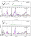 |
Fig. A.1. Spectra of SDSS J002023.12+074041.1 and SDSS J003411.37-032618.2, with specfit analysis results. For each spectrum, the top panel shows the full spectrum as a function of rest-frame wavelength, after normalization at 1350 Å. The actual continuum ranges employed in the fitting of the three spectral regions discussed in the paper are marked. The bottom panels show the decomposition of the blends. Black lines: observed spectrum under continuum subtraction. Magenta dashed lines: full model of the observed spectrum. Thick black lines: BC of SiIV, CIV, HeIIλ1640, AlIII and SiIII]. Blue lines: blue-shifted components of SiIV+OIV], CIV and HeIIλ1640. Grey lines: faint lines affecting the blends or AlIII BLUE component. |
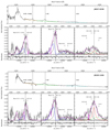 |
Fig. A.1. continued. |
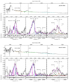 |
Fig. A.1. continued. |
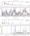 |
Fig. A.1. continued. |
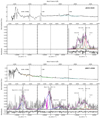 |
Fig. A.1. continued. |
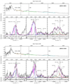 |
Fig. A.1. continued. |
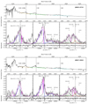 |
Fig. A.1. continued. |
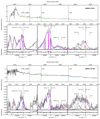 |
Fig. A.1. continued. |
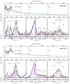 |
Fig. A.1. continued. |
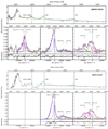 |
Fig. A.1. continued. |
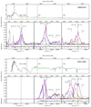 |
Fig. A.1. continued. |
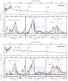 |
Fig. A.1. continued. |
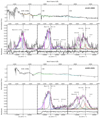 |
Fig. A.1. continued. |
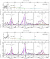 |
Fig. A.1. continued. |
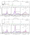 |
Fig. A.1. continued. |
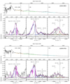 |
Fig. A.1. continued. |
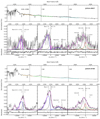 |
Fig. A.1. continued. |
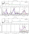 |
Fig. A.1. continued. |
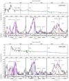 |
Fig. A.1. continued. |
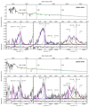 |
Fig. A.1. continued. |
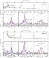 |
Fig. A.1. continued. |
Appendix B: Consideration on the spectral appearance of sample sources
Martinez-Aldama et al. (2018) carried out a very thorough descriptive analysis of the xA spectra. The spectra of the present sample resemble the composite spectrum shown by those authors. We therefore limit ourselves to a few remarks.
BAL QSOs. J0252−0420, an example of this type of sources, presents strong and prominent absorptions mainly between 1400 Å and 1550 Å. The absorption wipes out the emissions in these regions and inhibits their interpretation. We have 6 sources with this characteristic in our sample (as specified in Col. 9 of Table 1). We measured the regions that seem less affected but BAL QSOs are not considered for further analysis, save for the general comment reported below.
The FWHM(AlIII) of the BAL sources is predominantly above the sample mean with the lowest value 2788 km s−1 for J1516+0029 and the highest 4272 km s−1 for J1205+0201 (also the highest value of the sample), although the EW(AlIII) values are consistent with the average for the non-BAL sample. If we compare our available AlIII flux ratios this would lead us to super solar values ∼15 Z⊙, as already derived by Baldwin et al. (1996).
"mini-BALs". In addition to the broad, strong absorptions in sources classified as BAL QSOs, we also found the presence of strong narrow absorptions in 8 of our spectra. These absorptions are mainly in the 1400 Å and 1550 Å regions and blur out just a section of the emission, so that we can still retrieve the emission profile. J0034−0326 is an example where absorptions blur out small radial velocity sections in both the aforementioned spectral regions. The metallicity of these sources remains consistent with the median value of the sample.
Strong BC/weak lined quasars. The values of the equivalent width of all lines save Lyα are small, including the CIV BLUE, with a distribution of the full CIV profile (BC+BLUE) peaked around 10 Å, with a small dispersion. Half of the sample sources qualify as "weak-lined quasars" (Diamond-Stanic et al. 2009; Luo et al. 2015; Marziani et al. 2016). Sources that have prominent CIV BC with respect to CIV BLUE are present in our sample but are labeled as outliers or borderline sources. Two cases in point are J1231+0725 and J2116+0441.
J0858+0152 is measured as one of the most metal rich sources in the sample of S21. It visually meets all the indicators signaling high Z: ratio SiIV/CIV ∼1, extreme AlIII/SiIII], low WCIV. The result concerning the metallicity relies, however, on the continuum placement in the region at ≈1350 Å, where severe blending with [OI]λ6300 and Si IIλ1814 and ultimately with the very extended Lyα red wing makes it difficult to identify the continuum level properly.
All Tables
All Figures
|
Fig. 1. Redshift distribution of the sample as a function of the absolute i-band magnitude Mi. The gray-scale squares show the Lyke et al. (2020) data, binned over small bins in z and Mi. The pink squares identify the sample used in this work. Upper panel: normalized redshift distribution. The pink histogram shows the corrected redshift adopted in this paper (see Sect. 3.1). Right panel: normalized absolute i-band magnitude distributions for both Lyke et al. (2020) and our sample. |
| In the text | |
|
Fig. 2. SDSS J092919.45+033303.4, with specfit analysis results. Top panel: full spectrum as a function of rest-frame wavelength, after normalization at 1350 Å. The actual continuum ranges employed in the fitting of the three spectral regions discussed in the paper are marked. Bottom panels: decomposition of the blends. Black lines: observed spectrum under continuum subtraction. Magenta dashed lines: full model of the observed spectrum. Thick black lines: BC of SiIV, CIV, HeIIλ1640, AlIII and SiIII]. Blue lines: blue-shifted components of SiIV + OIV], CIV and HeIIλ1640. Green line: FeIII(UV34) template. Red line: CIII] emission. Gray lines: faint lines affecting the blends or AlIII BLUE component. |
| In the text | |
|
Fig. 3. Observed and synthetic spectra of J0929+0333. The abscissa corresponds to the rest frame wavelength in Å; the ordinate is the flux normalized to the continuum at 1350 Å. Left: black line: observed spectra minus the continuum; pink: model fit using specfit. The BC emission of AlIII and SiIII] are shown in purple, CIII] emission is shown in red, and the Fe III template is shown in green. Right: black line: the synthetic spectrum composed of the sum of the emission line components plus noise. The BC emission of AlIII (the sum of the doublet) and SiIII] are again shown in purple, the CIII] emission and the Fe III template are shown in red and green, respectively. |
| In the text | |
|
Fig. 4. Example of the 1550 Å region used for profile ratio measurements. The Figure shows in black the observed spectra minus the continuum. The red dashed lines indicate the rest frame wavelength of CIV and He II, the gray area surrounding these lines show the ±1000 km s−1 range of intensity measurement. The blue dashed lines indicate the BLUE emissions and are −4000 km s−1 from their broad component companion, the gray area surrounding these lines also show the ±1000 km s−1 range of measurement. Abscissa correspond to the rest frame wavelength in Å and ordinate normalized flux. |
| In the text | |
|
Fig. 5. Distribution (top) and individual (bottom) values of intensity ratios between prominent lines not used to estimate metallicity. The two panels on the right (AlIII/SiIII] and CIII]/SiIII]) show the ratios involved in the identification of xA sources. Vertical solid lines identify the mean value of the distribution. Dashed lines are set to 1 for the SiIII]/He II and CIII]/He II distributions, and 0.5 and 1.0 for the AlIII/SiIII] and CIII]/SiIII] distributions respectively, according to the UV selection criteria for the xA (Sect. 4.2). |
| In the text | |
|
Fig. 6. Distribution (top) and individual (bottom) values of intensity ratios of the broad components used as diagnostics for Z involving HeIIλ1640 (left), and not involving HeIIλ1640 (right). Values are reported in Cols. 2 to 7 of Table 8. |
| In the text | |
|
Fig. 7. Intensity ratios for the BLUE components, shown in the same layout of the previous figures. Values are reported in Cols. 8 to 10 of Table 8. |
| In the text | |
|
Fig. 8. Relation between AlIIIλ1860/SiIII]λ1892 and CIII]λ1909/SiIII]λ1892 intensity ratios. The gray area corresponds to the parameter space occupied by xA objects. Outlying sources are shown in pink color. |
| In the text | |
|
Fig. 9. Correlations between diagnostic ratios for the broad and BLUE components (left lower matrix), and between physical parameters (right upper matrix). The pink dots are the outlier sources described in Sect. 4.2 and were not considered in the statistical analysis. Additionally, for each panel we excluded, if necessary, the objects with the highest dispersion from the main relation (black dots). The blue and green dots are the values considered for each relation, the solid lines show the linear fit, the shaded areas represent the confidence interval of the lineal regression. For each relation the Spearman correlation coefficient (r) is shown in the right top corner. |
| In the text | |
|
Fig. 10. Intensity ratios trends predicted by CLOUDY as a function of the logarithm of the metallicity, for fixed physical parameters U and nH. Left panel: ratios of low/intermediate ionization potential BC lines. Right panel: ratios for high ionization potential emissions (BLUE components). In both panels, the stars represent the ratios predicted by CLOUDY. The dashed lines are the interpolation between the CLOUDY values obtained with a cubic spline, the thick solid line segments in each trend line show the range of line ratios covered by our sample, according to the measured flux ratios. |
| In the text | |
|
Fig. 11. Distribution (top panels) and individual (bottom panels) values of line ratio metallicity estimate involving HeIIλ1640 using broad components (left) and BLUE components (right). |
| In the text | |
|
Fig. 12. Parameter space nH, U, Z. Data points in 3D space are elements in the grid of the parameter space selected for not being different from |
| In the text | |
|
Fig. 13. Left: parameter space nH, U, Z, as in Fig. 12, but for component BLUE. As in that case, data points were computed from the emission line ratios referring to the median values in Table 6. The individual contour line was smoothed with a Gaussian kernel. Right: the plane log U vs. log Z. The outer isophotal contours delimit the region χmin + 1, where the χmin is the value after smoothing with a Gaussian filter. The low- and high-ionization solutions are marked. |
| In the text | |
|
Fig. 14. Top, from left to right: relation between intensity ratios CIV/HeIIλ1640, AlIII/HeIIλ1640 and CIV/HeIIλ1640 BC computed with specfit and with profile ratio technique described in Sect. 5.1.1. Bottom: comparison of intensity ratios for (SiIV + OIV]])/HeIIλ1640 for the BLUE component. Sources with the largest discrepancy from the equality line are identified. |
| In the text | |
|
Fig. 15. From left to right: relation between intensity ratios CIV/HeIIλ1640, AlIII/HeIIλ1640, CIV/HeIIλ1640 BLUE, (SiIV + OIV]/)HeIIλ1640, and (SiIV + OIV]/)HeIIλ1640 BLUE for the 13 objects in common with S21. The labels identify sources with largest deviation from the 1:1 lines. |
| In the text | |
|
Fig. 16. Metallicity comparison of our two fitting methods. Abscissas corresponds to specfit results and the ordinates to profile ratio measurements results. Each panel shows the values per metallicity relation, top left corner indicates the Spearman correlation coefficient, the black solid line shows the equality line. Sources with the largest discrepancy from the equality line are discarded and identified as black dots. |
| In the text | |
|
Fig. 17. Left panel: difference in the metallicity estimates from the AlIII/HeIIλ1640 intensity ratio and from the CIV/HeIIλ1640 ratio of the broad component, as a function of ionization parameter and density. The difference remain significant at a 2σ confidence level down to Δlog Z = log Z(AlIII/HeIIλ1640) − log Z(CIV/HeIIλ1640) ≈0.3. Right: same, for difference in the metallicity estimates from the (SiIV + OIV])/HeIIλ1640 ratio (≈SiIV/HeIIλ1640) and from the C IV/HeIIλ1640 ratio. The two cases with red values are lower limits. |
| In the text | |
|
Fig. A.1. Spectra of SDSS J002023.12+074041.1 and SDSS J003411.37-032618.2, with specfit analysis results. For each spectrum, the top panel shows the full spectrum as a function of rest-frame wavelength, after normalization at 1350 Å. The actual continuum ranges employed in the fitting of the three spectral regions discussed in the paper are marked. The bottom panels show the decomposition of the blends. Black lines: observed spectrum under continuum subtraction. Magenta dashed lines: full model of the observed spectrum. Thick black lines: BC of SiIV, CIV, HeIIλ1640, AlIII and SiIII]. Blue lines: blue-shifted components of SiIV+OIV], CIV and HeIIλ1640. Grey lines: faint lines affecting the blends or AlIII BLUE component. |
| In the text | |
|
Fig. A.1. continued. |
| In the text | |
|
Fig. A.1. continued. |
| In the text | |
|
Fig. A.1. continued. |
| In the text | |
|
Fig. A.1. continued. |
| In the text | |
|
Fig. A.1. continued. |
| In the text | |
|
Fig. A.1. continued. |
| In the text | |
|
Fig. A.1. continued. |
| In the text | |
|
Fig. A.1. continued. |
| In the text | |
|
Fig. A.1. continued. |
| In the text | |
|
Fig. A.1. continued. |
| In the text | |
|
Fig. A.1. continued. |
| In the text | |
|
Fig. A.1. continued. |
| In the text | |
|
Fig. A.1. continued. |
| In the text | |
|
Fig. A.1. continued. |
| In the text | |
|
Fig. A.1. continued. |
| In the text | |
|
Fig. A.1. continued. |
| In the text | |
|
Fig. A.1. continued. |
| In the text | |
|
Fig. A.1. continued. |
| In the text | |
|
Fig. A.1. continued. |
| In the text | |
|
Fig. A.1. continued. |
| In the text | |
Current usage metrics show cumulative count of Article Views (full-text article views including HTML views, PDF and ePub downloads, according to the available data) and Abstracts Views on Vision4Press platform.
Data correspond to usage on the plateform after 2015. The current usage metrics is available 48-96 hours after online publication and is updated daily on week days.
Initial download of the metrics may take a while.