| Issue |
A&A
Volume 697, May 2025
Euclid on Sky
|
|
|---|---|---|
| Article Number | A14 | |
| Number of page(s) | 16 | |
| Section | Extragalactic astronomy | |
| DOI | https://doi.org/10.1051/0004-6361/202451868 | |
| Published online | 30 April 2025 | |
Euclid: The Early Release Observations Lens Search Experiment★
1
Institute of Physics, Laboratory of Astrophysics, Ecole Polytechnique Fédérale de Lausanne (EPFL), Observatoire de Sauverny,
1290
Versoix,
Switzerland
2
Max-Planck-Institut für Astrophysik,
Karl-Schwarzschild-Str. 1,
85748
Garching, Germany
3
SCITAS, Ecole Polytechnique Fédérale de Lausanne (EPFL),
1015
Lausanne,
Switzerland
4
INAF-Osservatorio Astronomico di Capodimonte,
Via Moiariello 16,
80131
Napoli, Italy
5
Institute of Cosmology and Gravitation, University of Portsmouth,
Portsmouth
PO1 3FX, UK
6
Institut de Ciències del Cosmos (ICCUB), Universitat de Barcelona (IEEC-UB),
Martí i Franquès 1,
08028
Barcelona, Spain
7
Institució Catalana de Recerca i Estudis Avançats (ICREA),
Passeig de Lluís Companys 23,
08010
Barcelona, Spain
8
Aix-Marseille Université, CNRS, CNES, LAM,
Marseille,
France
9
Institut d’Astrophysique de Paris, UMR 7095, CNRS, and Sorbonne Université,
98 bis boulevard Arago,
75014
Paris,
France
10
Dipartimento di Fisica e Astronomia “Augusto Righi” – Alma Mater Studiorum Università di Bologna,
via Piero Gobetti 93/2,
40129
Bologna, Italy
11
INAF – Osservatorio di Astrofisica e Scienza dello Spazio di Bologna,
Via Piero Gobetti 93/3,
40129
Bologna, Italy
12
Department of Physics “E. Pancini”, University Federico II,
Via Cinthia 6,
80126
Napoli, Italy
13
INFN section of Naples,
Via Cinthia 6,
80126
Napoli, Italy
14
Technical University of Munich, TUM School of Natural Sciences, Physics Department,
James-Franck-Str. 1,
85748
Garching, Germany
15
Institut de Recherche en Astrophysique et Planétologie (IRAP), Université de Toulouse, CNRS, UPS, CNES,
14 Av. Edouard Belin,
31400
Toulouse,
France
16
UCB Lyon 1, CNRS/IN2P3, IUF, IP2I Lyon,
4 rue Enrico Fermi,
69622
Villeurbanne,
France
17
Department of Astronomy, University of Cape Town, Rondebosch,
Cape
Town 7700, South Africa
18
STAR Institute, University of Liège, Quartier Agora,
Allée du six Août 19c,
4000
Liège,
Belgium
19
INFN-Sezione di Bologna,
Viale Berti Pichat 6/2,
40127
Bologna, Italy
20
Universitäts-Sternwarte München, Fakultät für Physik, Ludwig-Maximilians-Universität München,
Scheinerstrasse 1,
81679
München, Germany
21
Max Planck Institute for Extraterrestrial Physics,
Giessenbachstr. 1,
85748
Garching, Germany
22
INFN, Sezione di Lecce, Via per Arnesano, CP-193,
73100
Lecce, Italy
23
Department of Mathematics and Physics E. De Giorgi, University of Salento, Via per Arnesano, CP-I93,
73100
Lecce,
Italy
24
INAF-Sezione di Lecce, c/o Dipartimento Matematica e Fisica, Via per Arnesano,
73100
Lecce,
Italy
25
Department of Physics, Oxford University,
Keble Road,
Oxford
OX1 3RH, UK
26
Jodrell Bank Centre for Astrophysics, Department of Physics and Astronomy, University of Manchester,
Oxford Road,
Manchester
M13 9PL, UK
27
Max-Planck-Institut für Astronomie,
Königstuhl 17,
69117
Heidelberg, Germany
28
Department of Physics, Centre for Extragalactic Astronomy, Durham University,
South Road,
Durham
DH1 3LE, UK
29
Department of Physics, Institute for Computational Cosmology, Durham University,
South Road,
Durham
DH1 3LE, UK
30
INAF, Istituto di Radioastronomia,
Via Piero Gobetti 101,
40129
Bologna, Italy
31
University of Applied Sciences and Arts of Northwestern Switzerland, School of Engineering,
5210
Windisch,
Switzerland
32
Jet Propulsion Laboratory, California Institute of Technology,
4800 Oak Grove Drive,
Pasadena,
CA,
91109,
USA
33
Centro de Astrofísica da Universidade do Porto, Rua das Estrelas,
4150-762
Porto, Portugal
34
Instituto de Astrofísica e Ciências do Espaço, Universidade do Porto, CAUP, Rua das Estrelas,
4150-762
Porto, Portugal
35
School of Physical Sciences, The Open University,
Milton Keynes
MK7 6AA,
UK
36
Minnesota Institute for Astrophysics, University of Minnesota,
116 Church St SE,
Minneapolis,
MN
55455, USA
37
Dipartimento di Fisica “Aldo Pontremoli”, Università degli Studi di Milano,
Via Celoria 16,
20133
Milano, Italy
38
INAF-IASF Milano,
Via Alfonso Corti 12,
20133
Milano, Italy
39
Department of Physics and Astronomy, University of the Western Cape,
Bellville,
Cape Town,
7535, South Africa
40
Observatoire de Sauverny, Ecole Polytechnique Fédérale de Lausanne,
1290
Versoix,
Switzerland
41
David A. Dunlap Department of Astronomy & Astrophysics, University of Toronto,
50 St George Street,
Toronto, Ontario
M5S 3H4, Canada
42
Laboratoire d’Astrophysique de Bordeaux, CNRS and Université de Bordeaux, Allée Geoffroy St. Hilaire,
33165
Pessac,
France
43
Institut universitaire de France (IUF),
1 rue Descartes,
75231
PARIS CEDEX 05, France
44
Caltech/IPAC,
1200 E. California Blvd.,
Pasadena,
CA
91125, USA
45
Université Paris-Saclay, Université Paris Cité, CEA, CNRS, AIM,
91191
Gif-sur-Yvette, France
46
Université de Strasbourg, CNRS, Observatoire astronomique de Strasbourg,
UMR 7550,
67000
Strasbourg, France
47
Department of Physics, Université de Montréal,
2900 Edouard Montpetit Blvd,
Montréal, Québec
H3T 1J4, Canada
48
Instituto de Física de Cantabria, Edificio Juan Jordá, Avenida de los Castros,
39005
Santander,
Spain
49
Dipartimento di Fisica e Scienze della Terra, Università degli Studi di Ferrara,
Via Giuseppe Saragat 1,
44122
Ferrara, Italy
50
Departamento Física Aplicada, Universidad Politécnica de Cartagena,
Campus Muralla del Mar,
30202
Cartagena, Murcia,
Spain
51
Laboratoire univers et particules de Montpellier, Université de Montpellier, CNRS,
34090
Montpellier,
France
52
Kapteyn Astronomical Institute, University of Groningen,
PO Box 800,
9700
AV Groningen, The Netherlands
53
ESAC/ESA, Camino Bajo del Castillo,
s/n., Urb. Villafranca del Castillo,
28692
Villanueva de la Cañada, Madrid,
Spain
54
INAF-Osservatorio Astrofisico di Arcetri,
Largo E. Fermi 5,
50125
Firenze, Italy
55
Institute of Physics, Laboratory for Galaxy Evolution, Ecole Polytechnique Fédérale de Lausanne, Observatoire de Sauverny,
1290
Versoix,
Switzerland
56
School of Mathematics and Physics, University of Surrey, Guildford, Surrey,
GU2 7XH,
UK
57
INAF – Osservatorio Astronomico di Brera,
Via Brera 28,
20122
Milano, Italy
58
IFPU, Institute for Fundamental Physics of the Universe,
via Beirut 2,
34151
Trieste, Italy
59
INAF-Osservatorio Astronomico di Trieste,
Via G. B. Tiepolo 11,
34143
Trieste, Italy
60
INFN, Sezione di Trieste,
Via Valerio 2,
34127 Trieste, TS,
Italy
61
SISSA, International School for Advanced Studies,
Via Bonomea 265,
34136 Trieste, TS,
Italy
62
Dipartimento di Fisica e Astronomia, Università di Bologna,
Via Gobetti 93/2,
40129
Bologna, Italy
63
INAF-Osservatorio Astronomico di Padova,
Via dell’Osservatorio 5,
35122
Padova, Italy
64
Centre National d’Etudes Spatiales – Centre spatial de Toulouse,
18 avenue Edouard Belin,
31401
Toulouse Cedex 9, France
65
INAF-Osservatorio Astrofisico di Torino,
Via Osservatorio 20,
10025
Pino Torinese (TO), Italy
66
Dipartimento di Fisica, Università di Genova,
Via Dodecaneso 33,
16146, Genova,
Italy
67
INFN-Sezione di Genova,
Via Dodecaneso 33,
16146
Genova, Italy
68
Faculdade de Ciências da Universidade do Porto, Rua do Campo de Alegre,
4150-007
Porto, Portugal
69
Dipartimento di Fisica, Università degli Studi di Torino,
Via P. Giuria 1,
10125
Torino, Italy
70
INFN-Sezione di Torino,
Via P. Giuria 1,
10125
Torino, Italy
71
Mullard Space Science Laboratory, University College London, Holmbury St Mary,
Dorking, Surrey
RH5 6NT, UK
72
Centro de Investigaciones Energéticas, Medioambientales y Tecnológicas (CIEMAT),
Avenida Complutense 40,
28040
Madrid, Spain
73
Port d’Informació Científica,
Campus UAB, C. Albareda s/n,
08193
Bellaterra (Barcelona), Spain
74
Institute for Theoretical Particle Physics and Cosmology (TTK), RWTH Aachen University,
52056
Aachen,
Germany
75
INAF-Osservatorio Astronomico di Roma,
Via Frascati 33,
00078
Monteporzio Catone, Italy
76
Dipartimento di Fisica e Astronomia “Augusto Righi” – Alma Mater Studiorum Università di Bologna,
Viale Berti Pichat 6/2,
40127
Bologna, Italy
77
Instituto de Astrofísica de Canarias, Vía Láctea,
38205
La Laguna, Tenerife,
Spain
78
Institute for Astronomy, University of Edinburgh, Royal Observatory,
Blackford Hill,
Edinburgh
EH9 3HJ, UK
79
European Space Agency/ESRIN,
Largo Galileo Galilei 1,
00044 Frascati, Roma,
Italy
80
Université Claude Bernard Lyon 1, CNRS/IN2P3, IP2I Lyon, UMR 5822,
Villeurbanne
69100, France
81
Departamento de Física, Faculdade de Ciências, Universidade de Lisboa, Edifício C8, Campo Grande,
1749-016
Lisboa, Portugal
82
Instituto de Astrofísica e Ciências do Espaço, Faculdade de Ciências, Universidade de Lisboa, Campo Grande,
1749-016
Lisboa, Portugal
83
Department of Astronomy, University of Geneva,
ch. d’Ecogia 16,
1290
Versoix, Switzerland
84
INFN – Padova,
Via Marzolo 8,
35131
Padova, Italy
85
INAF-Istituto di Astrofisica e Planetologia Spaziali,
via del Fosso del Cavaliere, 100,
00100
Roma, Italy
86
Aix-Marseille Université, CNRS/IN2P3, CPPM,
Marseille,
France
87
Istituto Nazionale di Fisica Nucleare, Sezione di Bologna,
Via Irnerio 46,
40126
Bologna, Italy
88
FRACTAL S.L.N.E., calle Tulipán 2,
Portal 13 1A,
28231,
Las Rozas de Madrid, Spain
89
Institute of Theoretical Astrophysics, University of Oslo,
PO Box 1029
Blindern,
0315
Oslo,
Norway
90
Leiden Observatory, Leiden University,
Einsteinweg 55,
2333
CC Leiden, The Netherlands
91
Department of Physics, Lancaster University,
Lancaster,
LA1 4YB,
UK
92
Felix Hormuth Engineering,
Goethestr. 17,
69181
Leimen, Germany
93
Technical University of Denmark,
Elektrovej 327,
2800
Kgs. Lyngby, Denmark
94
Cosmic Dawn Center (DAWN),
Denmark
95
NASA Goddard Space Flight Center,
Greenbelt,
MD
20771, USA
96
Department of Physics and Astronomy, University College London,
Gower Street,
London
WC1E 6BT, UK
97
Department of Physics and Helsinki Institute of Physics,
Gustaf Hällströmin katu 2,
00014
University of Helsinki, Finland
98
Université de Genève, Département de Physique Théorique and Centre for Astroparticle Physics,
24 quai Ernest-Ansermet,
CH-1211
Genève 4, Switzerland
99
Department of Physics,
PO Box 64,
00014
University of Helsinki, Finland
100
Helsinki Institute of Physics, Gustaf Hällströmin katu 2, University of Helsinki,
Helsinki,
Finland
101
NOVA optical infrared instrumentation group at ASTRON,
Oude Hoogeveensedijk 4,
7991PD, Dwingeloo,
The Netherlands
102
Centre de Calcul de l’IN2P3/CNRS,
21 avenue Pierre de Coubertin
69627
Villeurbanne Cedex, France
103
Universität Bonn, Argelander-Institut für Astronomie,
Auf dem Hügel 71,
53121
Bonn, Germany
104
INFN-Sezione di Roma, Piazzale Aldo Moro 2, c/o Dipartimento di Fisica, Edificio G. Marconi,
00185
Roma,
Italy
105
Institut d’Astrophysique de Paris,
98bis Boulevard Arago,
75014
Paris,
France
106
Institut de Física d’Altes Energies (IFAE), The Barcelona Institute of Science and Technology, Campus UAB,
08193
Bellaterra (Barcelona), Spain
107
European Space Agency/ESTEC,
Keplerlaan 1,
2201
AZ Noordwijk, The Netherlands
108
School of Mathematics, Statistics and Physics, Newcastle University, Herschel Building,
Newcastle-upon-Tyne
NE1 7RU,
UK
109
DARK, Niels Bohr Institute, University of Copenhagen,
Jagtvej 155,
2200
Copenhagen, Denmark
110
Waterloo Centre for Astrophysics, University of Waterloo, Waterloo,
Ontario
N2L 3G1, Canada
111
Department of Physics and Astronomy, University of Waterloo,
Waterloo, Ontario
N2L 3G1, Canada
112
Perimeter Institute for Theoretical Physics,
Waterloo, Ontario
N2L 2Y5, Canada
113
Space Science Data Center, Italian Space Agency, via del Politecnico snc,
00133
Roma,
Italy
114
Institute of Space Science, Str. Atomistilor, nr. 409 M˘gurele,
Ilfov
077125, Romania
115
Universidad de La Laguna, Departamento de Astrofísica,
38206
La Laguna, Tenerife,
Spain
116
Dipartimento di Fisica e Astronomia “G. Galilei”, Università di Padova,
Via Marzolo 8,
35131
Padova, Italy
117
Institut für Theoretische Physik, University of Heidelberg,
Philosophenweg 16,
69120
Heidelberg, Germany
118
Université St Joseph; Faculty of Sciences,
Beirut,
Lebanon
119
Departamento de Física, FCFM, Universidad de Chile,
Blanco Encalada 2008,
Santiago,
Chile
120
Universität Innsbruck, Institut für Astro- und Teilchenphysik,
Technikerstr. 25/8,
6020
Innsbruck, Austria
121
Institut d’Estudis Espacials de Catalunya (IEEC), Edifici RDIT, Campus UPC,
08860
Castelldefels, Barcelona,
Spain
122
Satlantis, University Science Park,
Sede Bld 48940,
Leioa-Bilbao, Spain
123
Institute of Space Sciences (ICE, CSIC),
Campus UAB, Carrer de Can Magrans, s/n,
08193
Barcelona,
Spain
124
Centre for Electronic Imaging, Open University,
Walton Hall,
Milton Keynes
MK7 6AA,
UK
125
Instituto de Astrofísica e Ciências do Espaço, Faculdade de Ciências, Universidade de Lisboa, Tapada da Ajuda,
1349-018
Lisboa, Portugal
126
Universidad Politécnica de Cartagena, Departamento de Electrónica y Tecnología de Computadoras,
Plaza del Hospital 1,
30202
Cartagena, Spain
127
INFN-Bologna,
Via Irnerio 46,
40126
Bologna, Italy
128
Infrared Processing and Analysis Center, California Institute of Technology,
Pasadena,
CA
91125, USA
129
ICL, Junia, Université Catholique de Lille, LITL,
59000
Lille,
France
130
ICSC – Centro Nazionale di Ricerca in High Performance Computing, Big Data e Quantum Computing,
Via Magnanelli 2,
Bologna,
Italy
131
Department of Physics and Astronomy, University of British Columbia,
Vancouver,
BC
V6T 1Z1, Canada
★★ Corresponding author; This email address is being protected from spambots. You need JavaScript enabled to view it.
Received:
12
August
2024
Accepted:
22
February
2025
Abstract
We investigated the ability of the Euclid telescope to detect galaxy-scale gravitational lenses. To do so, we performed a systematic visual inspection of the 0.7 deg2 Euclid Early Release Observations data towards the Perseus cluster using both the high-resolution IE band and the lower-resolution YE , JE, and HE bands. Each extended source brighter than magnitude 23 in IE was inspected by 41 expert human
classifiers. This amounts to 12086 stamps of 10″ × 10″. We found 3 grade A and 13 grade B candidates. We assessed the validity of these 16 candidates by modelling them and checking that they are consistent with a single source lensed by a plausible mass distribution. Five of the candidates pass this check, five others are rejected by the modelling, and six are inconclusive. Extrapolating from the five successfully modelled candidates, we infer that the full 14 000 deg2 of the Euclid Wide Survey should contain 100 000−30 000+ 70 000 galaxy-galaxy lenses that are both discoverable through visual inspection and have valid lens models. This is consistent with theoretical forecasts of 170 000 discoverable galaxy-galaxy lenses in Euclid. Our five modelled lenses have Einstein radii in the range 0'.'68 < θE < 1″.24, but their Einstein radius distribution is on the higher side when compared to theoretical forecasts. This suggests that our methodology is likely missing small-Einstein-radius systems. Whilst it is implausible to visually inspect the full Euclid dataset, our results corroborate the promise that Euclid will ultimately deliver a sample of around 105 galaxy-scale lenses.
Key words: gravitational lensing: strong / methods: data analysis / methods: observational / galaxies: clusters: individual: Perseus
This paper is published on behalf of the Euclid Consortium.
Deceased
© The Authors 2025
 Open Access article, published by EDP Sciences, under the terms of the Creative Commons Attribution License (https://creativecommons.org/licenses/by/4.0), which permits unrestricted use, distribution, and reproduction in any medium, provided the original work is properly cited.
This article is published in open access under the Subscribe to Open model. This email address is being protected from spambots. You need JavaScript enabled to view it. to support open access publication.
1 Introduction
Strong gravitational lensing by massive galaxies offers a plethora of applications in both cosmology and astrophysics. Some notable examples include measuring the total mass of lens galaxies within the Einstein radius and disentangling the contributions from visible and dark matter components (e.g. Auger et al. 2009). When coupled with deep spectroscopic observations, it enables the placement of constraints on the stellar initial mass function of lens galaxies (e.g. Ferreras et al. 2010; Dutton & Treu 2014; Sonnenfeld et al. 2019). Thanks to the lensing magnification, strong gravitational lensing serves as a natural telescope to study lensed sources otherwise too faint or angularly too small to be detected (e.g. Hezaveh et al. 2013), and even to map their velocity field with unprecedented spatial resolution (e.g. Paraficz et al. 2018). Studying small-scale distortions of lensed images or arcs allows us to infer the presence of low-mass dark halos either in the lens or along the line of sight up to the source redshift, and in turn to study the properties of dark matter (e.g. Vegetti et al. 2010; O’Riordan et al. 2023; Gilman et al. 2024). Moreover, when the lensed source is time-variable, such as a quasar or a supernova, strong lensing offers an independent way of measuring the expansion rate of the Universe, H0 (Refsdal 1964; Wong et al. 2020; Shajib et al. 2023; Grillo et al. 2024; Pascale et al. 2025).
Lastly, the measurement of weak lensing shear from strong lensing images has been proposed as a potential cosmological probe (Birrer et al. 2017, 2018). A minimal model for the shear that is non-degenerate with lens model parameters was derived by Fleury et al. (2021), and this quantity was shown to be measurable in mock imaging data by Hogg et al. (2023). For high-precision cosmological constraints, however, a Euclid-sized dataset of O(105) strong lenses will be required.
Galaxy-scale strong lensing events are rare, with about one object out of thousands showing lensing features (Oguri & Marshall 2010; Collett 2015). In addition, these systems are small in angular terms, spanning between tenths of an arcsecond to a few arcseconds on the sky, and the lensed images of the sources (arcs, rings, and multiple point sources) are often hidden in the glare of the foreground lensing galaxy. Because lenses are rare, compact, and low-contrast objects, they are best discovered in deep, sharp, wide-field surveys. Euclid is exactly that (Euclid Collaboration: Mellier et al. 2025), and is the focus of the present work. In fact, lensed quasi-stellar object candidates have already been proposed from Euclid observations (Cuillandre et al. 2025b).
However, even with high-quality Euclid data, finding lenses remains challenging, not only because of the intrinsic rarity of strong lensing, but also because other non-lensing objects mimic the morphology of lenses (e.g. ring galaxies, galaxy mergers, spiral galaxies, or even random alignments). So far, the best methods for discovering lenses involve various flavours of con-volutional neural networks (see Petrillo et al. 2019; Jacobs et al. 2019; Stein et al. 2022; Savary et al. 2022; Rojas et al. 2022, to cite just a few) and, more recently, transformer networks (Thuruthipilly et al. 2022; Grespan et al. 2024; González et al. 2025). These networks require training sets that match the instrumental and astrophysical properties of the data very closely. Since we do not possess enough strong lens observations to constitute a training set, they have to be simulated, and the effectiveness of simulations in emulating nature is limited.
Machine learning methods are effective at finding lenses, but they are limited in terms of purity and false-positive rates. When false-positive rates are below 1%, such methods are useful for pre-selecting candidates from parent samples of tens or even hundreds of millions of galaxies (Cañameras et al. 2024). However, as the true – and poorly known – prevalence of lenses on the plane of the sky is very low, even a 1% false-positive rate can result in samples dominated by contaminants and unconvincing candidates. This is known as the base rate fallacy. As a result, human visual inspection is almost always necessary to fine-tune the network selection, although humans themselves sometimes have difficulty deciding on the validity of a lens candidate. This is especially true for small-Einstein-radius lenses.
Human visual inspection is useful on its own as a lens finding method but is limited by the volume of data that can be inspected by a team of experts in a reasonable amount of time. However, it has the advantage that it can pick up unusual lensing configurations (e.g. Keeton et al. 2000; Orban de Xivry & Marshall 2009; Collett & Bacon 2016) that, by definition, do not appear in large numbers in simulated training sets. It is also the only way to evaluate the prevalence of lenses on the plane of the sky and therefore the expected surface density of lensing systems for a given instrument, depth, spatial resolution, and wavelength. This has been attempted a few times in the past, for example in Hubble Space Telescope imaging (e.g. Faure et al. 2008; Pawase et al. 2014; Garvin et al. 2022). Rojas et al. (2023) also evaluated the performance of visual inspection with simulated data.
In the Early Release Observations (ERO) Lens Search Experiment (ELSE), we carried out a blind visual search of galaxy-scale strong lensing systems using some of the first data from the European Space Agency (ESA) satellite Euclid (Euclid Collaboration: Scaramella et al. 2022; Euclid Collaboration: Mellier et al. 2025). We focused on the Euclid ERO imaging of the Perseus galaxy cluster (Cuillandre et al. 2025a), and the only selection criterion for the extended sources to be inspected was a magnitude cut. Our search is therefore one of the broadest visual searches carried out so far in terms of pre-selection. The goals were: (1) to evaluate the performance of the Euclid telescope at finding galaxy-scale lenses; (2) to study the prevalence of strong lenses found by humans in Euclid; (3) to test the efficiency of human experts at finding lenses; and (4) to optimise future visual inspections that will be performed on lens candidates found by the automatic pipeline in Euclid.
The humans involved in this exercise are all lensing experts but were limited in number (41 exactly). Our work therefore contrasts with more intensive citizen science searches involving much larger numbers of humans but spanning a much smaller range in terms of expertise (Marshall et al. 2015; More et al. 2016).
Finally, assuming subtraction of the lens light, Euclid is predicted to find 170000 lenses in its six-year main survey (Collett 2015). We tested that prediction in this work, with the caveat that we did not perform any subtraction of the lens light. Thus, our results represent a lower bound in this regard.
We introduce the Euclid ERO observations of the Perseus cluster in Sect. 2. We then explain the methodology of the visual inspections in Sect. 3, along with the visualisation tools used. Afterwards, we report the results from the visual inspection in Sect. 4 and present the sample of lens candidates and some initial modelling in Sect. 5. In Sect. 6 we then compare the sample against the literature and estimate the number of lenses that will be discovered in the Euclid Wide Survey (EWS). We conclude in Sect. 7.
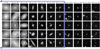 |
Fig. 1 9″.9 × 9″..9 VIS cutouts of galaxies randomly selected across different IE bins, ranging from the brightest galaxies with IE < 16 (leftmost) down to very faint systems with 24.5 < IE < 25 (rightmost). The blue arrow represents the magnitude cut used to select our parent sample. |
2 Data
The Euclid ERO programme (Euclid Early Release Observations 2024) targeted the Perseus galaxy cluster, obtaining very deep data of the central region of the cluster in 0.7 deg2, in the broad optical filter IE from the visible imager (VIS) instrument (Euclid Collaboration: Cropper et al. 2025), and the three broad filters YE, JE, and HE in the near-infrared from the Near-Infrared Spectrometer and Photometer (NISP) instrument (Euclid Collaboration: Jahnke et al. 2025).
These data were collected during the Euclid performance verification phase in September 2023 (Cuillandre et al. 2025a). All Euclid science observations adhere to a reference observing sequences (ROSs; Euclid Collaboration: Scaramella et al. 2022), which consists of four dithered exposures lasting 566 seconds each in the IE filter, and four dithered exposures of 87.2 seconds each in the YE, JE, and HE filters. Four ROSs were obtained for this field, with a total integration time of 7456.0 seconds in the IE filter and 1392.2 seconds in the YE, JE, and HE filters, achieving a depth 0.75 magnitudes deeper than that of the EWS, which relies on a single ROS (Euclid Collaboration: Scaramella et al. 2022). Therefore, these exceptional data reach a point-source depth of Ie = 27.3 (Ye, Je, He = 24.9) at 10 σ, with a 0″.16 (0″.48) full width at half maximum, and a surface brightness limit of 30.1 (29.2) mag arcsec−2. We refer the reader to Cuillandre et al. (2025a) for more details on the data reduction.
The astrometrically and photometrically calibrated imaging stacks across all four Euclid bands are accompanied by catalogues for compact sources produced using the tool SourceExtractor (Bertin & Arnouts 1996) on the ‘flattened’ stack, that is, with the low spatial frequencies removed (sky background and any Galactic cirrus or nebulae). Multi-wavelength catalogues including VIS, NISP, and ground-based Canada-France-Hawaii Telescope MegaCam photometry have been provided in Cuillandre et al. (2025b). After star–galaxy separation and limiting the analysis to sources with Ie < 23, we ended up with a parent sample of 12 086 objects, which was later used in the visual classification procedure. As shown in Fig. 1, the adopted magnitude cut is justified by the fact that sources at fainter magnitudes are compact and featureless. For the experiment, cutouts in the four Euclid bands of 9″.9 × 9″.9 (i.e. 99 × 99 pixels and 33 × 33 pixels in the VIS and NISP bands, respectively) were created using the flattened stacks.
3 Method
3.1 The visualisation tools
We used the visualisation tools prepared by Acevedo Barroso et al. (2025) to carry out the visual inspection1. The tools are based on the visualisation tools used in Savary et al. (2022) and Rojas et al. (2022), but re-implemented in the Qt 6 framework with extended functionality targeting the requirements of the Euclid ERO data. The two applications correspond to a mosaic viewer and a one-by-one sequential viewer, both presented in Fig. 2. The mosaic viewer displays rectangular mosaics of objects for the user to inspect. Then, the user is tasked with clicking on objects that show any signs of lensing. Additionally, the user is allowed to mark objects as ‘interesting, but not a lens’. This is exemplified in the left panel of Fig. 2. By contrast, the one-by-one sequential tool displays one object at the time and the user is tasked with classifying it into one of the following non-overlapping categories:
‘A’ indicates a sure lens: it shows clear lensing features and no additional information is needed.
‘B’ indicates a probable lens: it shows lensing features but additional information is required to verify it as a definite lens.
‘C’ indicates a possible lens: it shows lensing features, but they can be explained without resorting to gravitational lensing.
‘X’ indicates it is definitively not a lens.
‘Interesting’ indicates it is definitively not a lens but is interesting in some other way.
The grades A, B, and C are deemed as positive grades, whereas X and Interesting are deemed as negative. The one-by-one sequential tool is shown in the right panel of Fig. 2. Both tools allow the users to change the colour map used for the monochromatic images, as well as the function used to scale the pixel intensities. For every object to inspect, the tools generate three high-contrast images:
a monochromatic IE image at the VIS resolution of 0″.1 pixel−1;
a red-green-blue (RGB) composite image using the HE, YE, and IE bands, at the NISP resolution of 0″.3 pixel−1;
an RGB composite image using the HE, JE, and YE bands, at the NISP resolution of 0″.3 pixel−1.
Before creating the composite images, we re-projected the IE band data from the sky-coordinate system and resolution of the VIS instrument to the corresponding ones in the NISP instrument. This aligns the images and corrects for the different pixel scales between instruments. The experts were required to use the monochromatic high-resolution IE band, and the HE YE IE composite. The HE JE YE composite is not shown by default in the tools, but it is also available. Additionally, the users also have access to the individual NISP bands when using the one-by-one sequential tool. This is shown in Fig. 2.
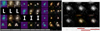 |
Fig. 2 Visualisation tools used for the visual inspection. Left panel: mosaic tool showing 12 sources in a 3 × 4 rectangular grid. The first object of the second row is marked as a lens candidate, whereas the second object of the third row is marked as interesting. Right panel: one-by-one sequential tool showing an object graded as C. Both tools show a monochromatic high-resolution IE band image, an HE YE IE RGB composite image, and a HE JE YE RGB composite image (in the second row for the one-by-one sequential tool). Both RGB composite images are at the NISP resolution. The one-by-one sequential tool also shows, in its first row, the three NISP bands: YE, JE, and HE. Users are only required to inspect the high-resolution IE monochromatic image and the HE YE IE composite image. |
3.2 The visual inspections
To make better use of the large number of strong lensing experts available for the visual inspection, we split the 41 experts into two non-overlapping teams. This allowed us to try different visual inspection schemes while still retaining enough experts per team for the classifications not to be dominated by noise. Team 1 comprises 22 experts, and Team 2 comprises 19. Both teams inspect the 12 086 cutouts described in Sect. 2, along with six extra cutouts of simulated lenses produced following the prescription of Euclid Consortium, Metcalf et al. (in prep). The introduction of simulated mocks tests the ability of the experts to identify lenses, and serves as a sanity check of their performance. The experts are not informed about the mocks in order to avoid any biases. The six simulated lenses can be seen in Fig. 3. Both teams are given two weeks per stage. There is no communication either between or within the teams, and their results are not combined until after the visual inspections are completed.
Both teams followed a two-stage approach. First, they focused on cleaning the parent sample of obvious non-lens contaminants. Then, they inspected the remaining sources in detail and settled on a final classification following the grades introduced in Sect. 3.1.
Team 1 first inspects the entire parent sample using the mosaic tool. This corresponds to 12 092 cutouts after adding the mock lenses. The experts were allowed to change the number of sources per page shown in the mosaic, with most experts observing between 20 and 42 sources per mosaic page. Afterwards, Team 1 reinspected all the objects selected in the first stage using the one-by-one sequential tool and assigning detailed classifications.
Simultaneously, Team 2 is further divided into three groups: two groups comprising six experts each and one group comprising seven. Each group inspects one third of the sources using the one-by-one sequential tool, while focusing on rejecting obvious contaminants. During the first stage, no detailed classification is required. Subsequently, all the selected sources are reinspected by Team 2 as a whole, using again the one-by-one sequential tool but assigning detailed classifications.
Afterwards, we aggregated the final classifications of each team independently. The output is a single final classification per team for every source. Thus, if more than half of the experts voted negatively, then the source was classified as a non-lens; otherwise, we classified it as the majority vote between A, B, and C. In the case of a tie between A and B, or A and C, A took precedence. This prioritisation reflects the expectation that experts will only vote for A if they are confident about the presence of lensing features. If there is a tie between B and C, we favoured C to minimise noise in the final B sample. In the event of a tie among all three positive classes, B was preferred.
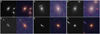 |
Fig. 3 Six simulated lenses as seen in the visualisation tools. The left side of each panel corresponds to the high-resolution IE band data, and the right to the HE YE IE composite image. The letter at the upper-left corner of each panel corresponds to the final joint grade given in the visual inspection. |
4 Visual inspection
The experts are anonymised at every stage of the analysis to avoid biasing the visual inspection results. We refer to the experts only by their expert ID, for example, ‘expert number 12’.
4.1 Team 1
The first stage of the visual inspection was completed by 20 out of the 22 experts that registered for Team 1. Figure 4 presents the number of lens candidates selected by each expert. We note that expert number 1 selected 15 σ more sources for reinspection when compared to the mean and standard deviation of the other experts from Team 1, which selected 106 ± 100 sources for reinspection. Figure 5 presents the distribution of votes with and without expert number 1. We observe that the number of sources selected only by a single expert drops by half when excluding the outlier expert. Consequently, we removed the classifications from expert number 1. This provided us with a generous selection for the second stage, in which we included every source chosen by any of the remaining experts, while also keeping the sample reasonably small. The total number of sources selected for inspection in stage 2 was 1233.
The second stage was completed by 17 out of the 22 experts. Figure A.1 presents the number of votes per grade per expert. Similarly, Table 1 presents the average number of votes per grade for every stage that used the one-by-one sequential tool. Both Fig. A.1 and Table 1 show that the experts of Team 1 were conservative when assigning the highest grade, A. This trend, however, was not the case for grades B and C, for which multiple experts assigned hundreds of votes in the 1233 sample. This indicates confusion among some experts for what constitutes a lens when the lensing features are not strikingly obvious. However, the experts with a large number of positive classifications were still a minority. Ultimately, the behaviour of all experts during the second stage was deemed acceptable and none of classifications were removed.
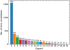 |
Fig. 4 Number of candidates selected in the first stage for reinspection by Team 1 using the mosaic tool. The experts were anonymised, and the expert IDs correspond only to the first stage of the visual inspection. |
4.2 Team 2
The first round of visual inspection was completed by 16 out of 19 experts involved in Team 2. The distribution among groups was as follows: five experts from both the first and second group, and another six from the third group. Figure A.2 and Table 1 summarise the behaviour of the experts during the inspection. The grades A and B were given to only a small number of sources and the overall proportion of positive votes was low. This is consistent with the task of removing the contaminants, which was the goal for stage 1. The visual inspection results are presented in Fig. 6. We discarded all the sources with a negative majority vote, except those that got at least one vote for A or B. This amounted to 691 sources for reinspection in stage 2.
The second stage of Team 2 was completed by 17 experts out of the 19 who registered. The grading behaviour of the experts is presented in Fig. A.3. A few of the experts gave a large number of positive grades, one grading positively 673 out of the 691. Still, most of the experts reserved the grades A and B for the few best candidates, and thus, we did not remove any experts. This is justified by the aggregation method introduced in Sect. 3.2, which relies on a majority vote to assign final grades.
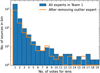 |
Fig. 5 Distribution of the number of positive votes for Team 1 before and after removing the outlier expert. Most of the sources received only one vote, and no object was selected by all the experts. |
Average number of votes per grade per expert for the inspections using the one-by-one sequential tool.
4.3 Time cost of the inspections
It took the experts of Team 1 between 1h 15m and 5h 15m to inspect the whole parent sample using the mosaic tool, with the median time being 2 h 45 m. By contrast, it took the experts from Team 2 between 1h30m to 3h30m with a median time of 2 h 15 m to inspect one third of the parent sample, but using the one-by-one sequential tool. The median time per source was 0.8 s and 2.0 s for Teams 1 and 2, respectively.
For the second stage, Team 1 experts took between 30 m and 3 h 30 m. The median time was 1 h 30 m, equivalent to 4.4 s per source. Finally, Team 2 experts took between 15 m and 2h, and the median was 45 m, which corresponds to 4.0 s per source. Overall, the time taken per source during the second stage was consistent for both teams. Given the filtering of the sample during the first stage, the time taken per source in the second stage corresponds more closely to the real time that a visual inspection would take on a preselected sample, for example the output of a convolutional neural network.
5 Results
5.1 The visual inspection candidates
We computed three grades for each source: two individual grades from Team 1 and Team 2 plus a final joint grade. The final grade of each team is determined by applying the scheme presented in Sect. 3.2 to their respective set of votes. The joint final grade is determined the same way but using the votes of both teams together in the computation, with the exception of sources that were rejected by one of the teams during the first stage. In that case, we added two negative votes to the classifications of the other team and calculated the final joint classification using the 19 votes.
Overall, we obtain three grade A, 13 grade B, and 52 grade C lens candidates from the final joint grades. We present a summary of the number of candidates per team in Fig. 7. Furthermore, we show the grade A and B candidates in Fig. 8, along with their three final grades: the final grade from Team 1, the final grade from Team 2, and the final joint grade (in yellow, cyan, and red, respectively). The grade C candidates, along with the sources selected by either team but rejected from the joint sample, are presented in a Zenodo appendix. We note that Team 1 found almost double the amount of grade A and grade B candidates, but about the same number of grade C candidates as Team 2. Moreover, all the candidates selected by Team 1 but rejected from the final sample were also rejected by Team 2 during the first stage. By contrast, most of the sources selected by Team 2 but rejected from the final sample were also rejected by Team 1 during the second stage. This suggests that using the one-by-one sequential tool to filter out the obvious non-lenses, as Team 2 did during the first stage, is in fact a more aggressive filter than using the mosaic tool to preselect candidates.
5.2 Modelling of the lens candidates
We further assessed the validity of the 16 grade A and B candidates by modelling the lens galaxy light and mass distribution, and surface brightness distribution of the lensed source. We did this using the pronto software (Vegetti & Koopmans 2009; Rybak et al. 2015a,b; Rizzo et al. 2018; Ritondale et al. 2019; Powell et al. 2021). We used a singular isothermal ellipsoid (SIE) density profile to describe the mass distribution of the galaxy, a composite of three Sérsic profiles for the lens galaxy light, and a pixelated, free-form reconstruction of the source surface brightness distribution. The parameters for the lens light and mass models are found through a non-linear optimisation using MultiNest (Feroz et al. 2009). For each set of light and mass parameters, the surface brightness distribution of the source is solved for linearly, up to some regularisation condition, which, in this case, penalises large gradients in the source. The strength of this regularisation is itself a non-linear parameter. The full model has 23 free parameters.
We used a circular mask centred on the lensing galaxy and large enough to enclose what are assumed to be lensed images. We also used the positions of these assumed lensed images as an input to the optimisation scheme. After selecting two, three, or four positions in the image plane, the non-linear optimiser will only accept models where these image plane positions have a root mean square separation in the source plane below some tolerance, in this case 1 arcsec. This removes the need to fine-tune the initial modelling conditions, since only combinations of lens parameters that focus the source are accepted. The large tolerance of 1 arcsec also prevents the subjective choice of image positions from placing strict restrictions on the model.
After the optimisation, we checked each model against three criteria to determine if its data are well described by a strong lensing model. These criteria are:
Is there an SIE critical curve that can enclose or exclude the right number of bright components in the image plane?
Is the centroid of this critical curve consistent with that of the light profile?
Is the reconstructed source surface brightness distribution consistent with a compact, focused object, inside a caustic?
Given the small sample size, the evaluation of these criteria is done in a qualitative basis through the visual inspection of the models (see Appendix B). A systematic and quantitative assessment requires evaluating these criteria against realistic simulations where the ground-truth is known, which is beyond the scope of this work.
Five of the 16 grade A and B candidates are found to have valid lens models according to the criteria above. Six candidates cannot be determined as lenses with the available data, and a final five candidates do not have valid lens models. For the five valid candidates, we measure Einstein radii in the range 0″.68–1″.24. The result for one valid candidate is shown, as an example, in Fig. 9; the rest are shown in Appendix B. The results of the visual inspection and modelling are summarized in Table 2.
 |
Fig. 6 Results from Team 2 during the first stage. Left: histogram of the ratio of negative votes versus the total number of classifications for the source. The sources with a ratio of negative votes lower than 0.5 were selected for stage 2. Right: total number of sources that received a given number of votes for a given classification. Most of the sources had zero votes for A, B, and C. All sources with at least one vote for A or B were also selected for stage 2. |
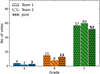 |
Fig. 7 Distribution of final grades for each team and for the joint classification. |
6 Discussion
6.1 The lens candidates in the literature
We crossmatched the sky coordinates of the 68 lens candidates against the Strong Lens Database (SLED; Vernardos et al., in prep.), a database of gravitational lenses, lens candidates, and known contaminants, encompassing more than 20000 entries. We found no matches between our sample and the database. Furthermore, the database indicates that there have been no lens searches in the area, since the closest match is more than 6° away. This is expected given that the Perseus cluster is near the Galactic plane, and thus, is not generally targeted by large-scale optical galaxy surveys.
Nonetheless, Li et al. (2024) have performed a lens search in some of the ERO fields, including the Perseus cluster, in order to test the lens detection algorithm to be used by the Chinese Space Station Telescope (CSST) team. For that purpose, they used the high-resolution media images published by ESA2. They found four lens candidates in the Perseus cluster and reported the pixel coordinates in the TIFF image. Three of those candidates are included in our parent sample and were selected by Team 1 for reinspection in the second stage. However, all of them were rejected in the second stage. A smaller committee of experts inspected the fourth candidate and ultimately rejected it. Thus, we believe that none of the Li et al. (2024) candidates in the Perseus cluster are lenses. The lack of real lenses in their sample is likely a consequence of using the lower-resolution TIFF images and the fact that their model was not trained to detect lenses in Euclid data. Therefore, the false positives in the Perseus cluster do not necessarily reflect on the potential performance of the algorithm in CSST data.
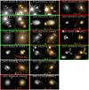 |
Fig. 8 Mosaic of the grade A and B lens candidates from the visual inspection. For each candidate we show the high-resolution IE band cutout in the left panel, and the lower-resolution HE YE IE composite image in the right panel. The final grades by Team 1, Team 2, and the final joint grade are shown in yellow, cyan, and red, respectively. No grade is shown if one of the sources was rejected by a team during the first stage of the visual inspection. The green borders highlight candidates with valid models, and red borders candidates rejected due to the modelling. |
6.2 The expected prevalence of ELSE lenses
Collett (2015, C15 hereafter) forecasts that 15 000 deg2 of Euclid imaging should contain 170000 strong gravitational lenses. Naively scaling down to the 0.7 deg2 Perseus field gives an expectation of eight galaxy-galaxy lenses, of which six should have IE < 23. We have three grade A and 13 grade B candidates, of which five have a valid lens model, and six are indeterminate. Despite the small number statistics, it is clear that our results and the C15 forecasts are broadly consistent. As well as the Poisson noise, our limited understanding of the discovery selection function, and the lack of spectroscopic redshift confirmation of our candidates makes it impossible to precisely compare our absolute number of lenses with the forecast population.
The median Einstein radius forecast in C15 is 0″.65, whereas the smallest Einstein radius of the five lenses with valid models in Sect. 5.2 is 0″.68. This tension is alleviated somewhat by accounting for the fact we only look at lenses with Ie < 23: by excluding the faintest lenses we prefer higher-mass or lower-redshift lenses, both of which result in larger Einstein radii. After applying this cut, the forecast median Einstein radius increases to 0″.75. Figure 10 shows the expected number of lenses in 0.7 deg2 of Euclid data, their Einstein radius distribution, and the Einstein radius distribution of successfully modelled ELSE candidates. The C15 forecasts assumed that the lens galaxy light would be subtracted, which is very helpful for finding small-Einstein-radius lenses: we have not done this. In future work, we will calibrate this selection function using simulations (Rojas et al., in prep.); in this study we used a toy model to estimate it. We assumed that the shape of the underlying Einstein radius population follows the Euclid forecasts of C15, and that the visual inspection introduced a selection function in the form of a step function, we detect every lens above a threshold Einstein radius (θmin) and none below this threshold. Using Bayes’ theorem, we infer P(θmin) given that we discovered five lenses and the lowest Einstein radius is in the range 0″.65–0″.70.
We used a Monte Carlo simulation to draw many realisations of five Einstein radii but varied the discovery threshold, assuming a uniform prior on the discovery threshold, θmin. We find that the threshold is  arcsec at 68% confidence. This corresponds to a forecast total population of
  lenses in the full Euclid dataset that are discoverable with visual inspection without lens light subtraction and with lens IE < 23. Moreover, scaling down the area to 0.7 deg2 the forecast predicts approximately five lenses, coinciding with the five lens candidates with good models.
Grade A and B candidates with magnitude, modelling status, and Einstein radii when available.
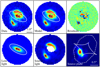 |
Fig. 9 Modelling results for one of the five valid candidates, EUCL J031741.85+412702.8. The six panels show, from left to right, top to bottom: the VIS cutout data, masked to a circle around the object; the model lens light and lensed source light distributions, convolved with the point spread function model; the normalised residuals on a colour scale between −3 σ and 3 σ; the lens light only; the lensed source light only, with the brightest parts of the lens light masked; and the reconstructed source plane model. The solid and dashed white ellipses in the image plane are the tangential and radial critical curves, with the corresponding caustics shown in the source plane. The image plane frames all have the same scale, as indicated in the first frame. |
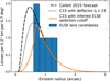 |
Fig. 10 Comparison of the number of lenses and their Einstein radius distribution of successfully modelled ELSE candidates (blue histogram), and the forecasts of Collett (2015) rescaled to 0.7 deg2 (dotted black line). The dotted black line is a prediction, not a fit. The orange ‘cutoff’ line is a modification of the Collett (2015) forecasts to account for the selection function arising from our methodology missing small-Einstein-radius lenses. |
6.3 The prevalence of ELSE lenses
We extrapolated the five lens candidates with valid lens models found in the ERO Perseus field to the entire EWS. For this, we made three key assumptions:
We have found all the discoverable lenses with IE < 23 within the ERO Perseus field.
The average number density of sources with IE < 23 in the EWS is the same as in the ERO Perseus field: ~ 17 000 extended sources per deg23.
The likelihood that a given source within the EWS exhibits lensing features mirrors that of the sources within the parent sample.
We defined a lens as discoverable if it can be identified via expert visual inspection and a valid lens model can be found for it. This assumption means that, in fact, we are mostly estimating the prevalence of larger Einstein radius lenses, which are easier to model and experts will identify more easily. However, small-Einstein-radius lenses can still be identified if the source is bright and the geometry of the lensed images is particularly evident; for example, the mock lens in the bottom right panel of Fig. 3, which has an Einstein radius of 0″.49, but also a typical quad geometry, was still graded A by the experts. Furthermore, given the increased depth of the ERO Perseus field data compared to the EWS (0.75 magnitudes), we simulated cutouts for the 16 lens candidates with the typical S/N of the EWS. We observe that the lensing features are still visible and clearly identifiable in the shallower cutouts. Consequently, we assumed that they would had been identified in the shallower EWS.
Under the key assumptions above, the prevalence of ELSE lenses in the EWS can be estimated as follows. The likelihood P(k) of finding k lenses among n trialled sources is given by the hypergeometric distribution
 (1)
(1)
where K and N are the total numbers of lenses and sources in the EWS. Using the second assumption, we estimate the total number of extended sources with IE < 23 in the 14 000 deg2 of the EWS to be N = 242 000 000. The number of trialled sources was n = 12 086, and the number of discoverable lenses was k = 5. We could then compute the posterior probability, P(K), using Bayes’ theorem (i.e. P(K|k) ∝ P(k|K)P(K)). We assumed that the prior probability of K, P(K), is such that the ratio K/N is distributed uniformly in log-space between 10−10 and unity. Overall, we expect  ELSE-type lenses in the entire EWS. The posterior distribution P(K) is presented in Fig. 11, with the 68% confidence interval highlighted in light blue. Figure 11 also shows in orange the forecast of C15 as described in the previous section, which lies inside the confidence range of our estimate, showing a good agreement between the forecast and our estimate.
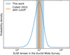 |
Fig. 11 Posterior probability density distribution of our estimation of the number of ELSE lenses in the EWS. The blue-shaded region marks the 68% confidence interval of our estimation: |


7 Conclusions
In this work, we have investigated the performance of the Euclid telescope for detecting galaxy-scale gravitational lenses. We employed 41 experts to carry out a blind visual search for lenses in the Euclid ERO data of the Perseus cluster. The search yielded 3 grade A and 13 grade B lens candidates.
We modelled the 16 candidates to test whether the observed VIS images are consistent with a single background galaxy lensed by a simple, plausible lens. We have obtained convincing models for five of the candidates. Modelling for six of the candidates produced inconclusive results, whilst five of the visual inspection candidates are definitively non-lenses according to our modelling.
We extrapolated the five candidates with valid lens models to the entire EWS and estimated the number of lenses in it that are discoverable with visual inspection and can be confirmed through modelling of the VIS data. This extrapolation yields  lenses in the full EWS. This is broadly consistent with the 170 000 forecast by C15.
Even though our magnitude cut of IE < 23 effectively removes many of the small-Einstein-radius objects, the distribution of Einstein radii in our modelled sample is still on the higher side when compared to C15, indicating that we are either unable to identify small-Einstein-radius systems in the visual inspections or unable to model them under our simplifying assumptions. Assuming a step function cutoff in Einstein radius, we inferred the cutoff point to be  arcsec; below this, our methodology is likely missing most of the lens candidates. Convolving our inferred cutoff with the Collett (2015) Euclid population, we now predict that
  galaxy-scale lenses will be detected in the whole EWS (assuming that the same visual inspection discovery and modelling methodology are performed on the entire dataset). Down-scaling to the 0.7 deg2 visually inspected in this work gives approximately five lenses, which is in perfect accordance with the five lens candidates with valid models.
This sample represents the first gravitational lenses reported in this patch of the sky, and some of the first lenses discovered with Euclid data. There is tentative evidence that we are missing small-Einstein-radius lenses, so future work will be necessary to develop identification techniques targeting small-Einstein-radius lens candidates. There are also substantial challenges in how we scale up from this field to the full dataset: blind visual inspection of 14 000 deg2 is implausible. Neural networks and citizen science are both likely to be needed to reduce the sample to a manageable size.
Even without spectroscopic confirmation of our candidates, our simple lens modelling provides compelling evidence that at least five of them are indeed strong gravitational lenses. These results are hugely promising for the future of strong lensing science with Euclid. Forecasts and early data both now point to the discovery of 105 or more gravitational lenses in the full Euclid dataset.
Data availability
Supplementary materials showing the lens candidates discovered in the search but not included in the main sample are available on Zenodo, at https://zenodo.org/records/14946028
Acknowledgements
This work has made use of the Early Release Observations (ERO) data from the Euclid mission of the European Space Agency (ESA), 2024, https://doi.org/10.57780/esa-qmocze3. The Euclid Consortium acknowledges the European Space Agency and a number of agencies and institutes that have supported the development of Euclid, in particular the Agenzia Spaziale Italiana, the Austrian Forschungsförderungsgesellschaft funded through BMK, the Belgian Science Policy, the Canadian Euclid Consortium, the Deutsches Zentrum für Luft- und Raumfahrt, the DTU Space and the Niels Bohr Institute in Denmark, the French Centre National d’Etudes Spatiales, the Fundação para a Ciência e a Tecnologia, the Hungarian Academy of Sciences, the Ministerio de Ciencia, Innovación y Universidades, the National Aeronautics and Space Administration, the National Astronomical Observatory of Japan, the Netherlandse Onderzoekschool Voor Astronomie, the Norwegian Space Agency, the Research Council of Finland, the Romanian Space Agency, the State Secretariat for Education, Research, and Innovation (SERI) at the Swiss Space Office (SSO), and the United Kingdom Space Agency. A complete and detailed list is available on the Euclid web site (www.euclid-ec.org). J. A. A. B., B. C., and F. C. acknowledge support from the Swiss National Science Foundation (SNSF). C. O’R thanks the Max Planck Society for support through a Max Planck Lise Meitner Group. C. T. and V. B. acknowledge the INAF grant 2022 LEMON. T. E. C. is funded by a Royal Society University Research Fellowship. S. H. S. thanks the Max Planck Society for support through the Max Planck Fellowship. This research is supported in part by the Excellence Cluster ORIGINS which is funded by the Deutsche Forschungsgemeinschaft (DFG, German Research Foundation) under Germany’s Excellence Strategy – EXC-2094 – 390783311. This project has received funding from the European Research Council (ERC) under the European Union’s Horizon 2020 research and innovation programme (LensEra: grant agreement No. 945536 and LENSNOVA: grant agreement No. 771776).
Appendix A Expert classifications in visual inspections
We show in this appendix the detailed classifications given by the experts when using the one-by-one sequential tool.
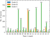 |
Fig. A.1 Classifications given by Team 1 during the second stage of the visual inspection. Each expert inspected 1221 sources and assigned the grades introduced in Sect. 3.1. Negative grades (X) were not included, for the sake of simplicity. The expert IDs correspond only to the second stage. |
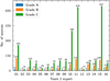 |
Fig. A.2 Classifications given by Team 2 during the first stage of the visual inspection. Each expert inspected about 4030 sources and assigned the grades introduced in Sect. 3.1. Negative grades (X) were not included, for the sake of simplicity. The expert IDs correspond only to the first stage. |
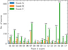 |
Fig. A.3 Classifications given by Team 2 during the second stage of the visual inspection. Each expert inspected 691 sources and assigned the grades introduced in Sect. 3.1. Negative grades (X) were not included, for the sake of simplicity. The expert numbers correspond only to the second stage. |
Appendix B Modelling results
The results of modelling all 16 grade A and B candidates are shown in Figs. B.1 to B.3.
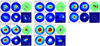 |
Fig. B.1 Modelling results for all five of the candidates that have valid lens models. Panels (A): VIS cutout data, masked to a circle around the object. Panels (B): Model lens light and lensed source light distributions, convolved with the point spread function model. Panels (C): Normalised residuals on a colour scale between −3 σ and 3 σ. Panels (D): Lens light only. Panels (E): Lensed source light only, with the brightest parts of the lens light masked. Panels (F): Reconstructed source plane model. The solid and dashed white ellipses in the image planes are the tangential and radial critical curves, with the corresponding caustics shown in the source plane. The image plane frames all have the same scale, which is indicated in the first frame. |
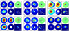 |
Fig. B.2 Modelling results for the six candidates for which we cannot determine their lensing status by modelling the current data. Mosaics follow the same layout as Fig. B.1. |
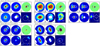 |
Fig. B.3 Modelling results for the five candidates that do not have valid lens models. Mosaics follow the same layout as Fig. B.1. |
References
- Acevedo Barroso, J. A., Clément, B., Courbin, F., et al. 2025, A&A submitted [arXiv:2503.10610] [Google Scholar]
- Auger, M. W., Treu, T., Bolton, A. S., et al. 2009, ApJ, 705, 1099 [Google Scholar]
- Bertin, E., & Arnouts, S. 1996, A&AS, 117, 393 [NASA ADS] [CrossRef] [EDP Sciences] [Google Scholar]
- Birrer, S., Welschen, C., Amara, A., & Refregier, A. 2017, J. Cosmology Astropart. Phys., 2017, 049 [Google Scholar]
- Birrer, S., Refregier, A., & Amara, A. 2018, ApJ, 852, L14 [Google Scholar]
- Cañameras, R., Schuldt, S., Shu, Y., et al. 2024, A&A, 692, A72 [NASA ADS] [CrossRef] [EDP Sciences] [Google Scholar]
- Collett, T. E. 2015, ApJ, 811, 20 [NASA ADS] [CrossRef] [Google Scholar]
- Collett, T. E., & Bacon, D. J. 2016, MNRAS, 456, 2210 [CrossRef] [Google Scholar]
- Cuillandre, J.-C., Bertin, E., Bolzonella, M., et al. 2025a, A&A, 697, A6 (Euclid on Sky SI) [Google Scholar]
- Cuillandre, J.-C., Bolzonella, M., Boselli, A., et al. 2025b, A&A, 697, A11 (Euclid on Sky SI) [Google Scholar]
- Dutton, A. A., & Treu, T. 2014, MNRAS, 438, 3594 [NASA ADS] [CrossRef] [Google Scholar]
- Euclid Collaboration (Scaramella, R., et al.) 2022, A&A, 662, A112 [NASA ADS] [CrossRef] [EDP Sciences] [Google Scholar]
- Euclid Collaboration (Cropper, M. S., et al.) 2025, A&A, 697, A2 (Euclid on Sky SI) [Google Scholar]
- Euclid Collaboration (Jahnke, K., et al.) 2025, A&A, 697, A3 (Euclid on Sky SI) [Google Scholar]
- Euclid Collaboration (Mellier, Y., et al.) 2025, A&A, 697, A1 (Euclid on Sky SI) [Google Scholar]
- Euclid Early Release Observations 2024, https://doi.org/10.57780/esa-qmocze3 [Google Scholar]
- Faure, C., Kneib, J.-P., Covone, G., et al. 2008, ApJS, 176, 19 [NASA ADS] [CrossRef] [Google Scholar]
- Feroz, F., Hobson, M. P., & Bridges, M. 2009, MNRAS, 398, 1601 [NASA ADS] [CrossRef] [Google Scholar]
- Ferreras, I., Saha, P., Leier, D., Courbin, F., & Falco, E. E. 2010, MNRAS, 409, L30 [NASA ADS] [CrossRef] [Google Scholar]
- Fleury, P., Larena, J., & Uzan, J.-P. 2021, J. Cosmology Astropart. Phys., 2021, 024 [Google Scholar]
- Garvin, E. O., Kruk, S., Cornen, C., et al. 2022, A&A, 667, A141 [NASA ADS] [CrossRef] [EDP Sciences] [Google Scholar]
- Gilman, D., Birrer, S., Nierenberg, A., & Oh, M. S. H. 2024, MNRAS, 533, 1687 [Google Scholar]
- González, J., Holloway, P., Collett, T., et al. 2025, arXiv e-prints [arXiv:2501.15679] [Google Scholar]
- Grespan, M., Thuruthipilly, H., Pollo, A., et al. 2024, A&A, 688, A34 [NASA ADS] [CrossRef] [EDP Sciences] [Google Scholar]
- Grillo, C., Pagano, L., Rosati, P., & Suyu, S. H. 2024, A&A, 684, L23 [NASA ADS] [CrossRef] [EDP Sciences] [Google Scholar]
- Hezaveh, Y. D., Marrone, D. P., Fassnacht, C. D., et al. 2013, ApJ, 767, 132 [NASA ADS] [CrossRef] [Google Scholar]
- Hogg, N. B., Fleury, P., Larena, J., & Martinelli, M. 2023, MNRAS, 520, 5982 [Google Scholar]
- Jacobs, C., Collett, T., Glazebrook, K., et al. 2019, ApJS, 243, 17 [Google Scholar]
- Keeton, C. R., Mao, S., & Witt, H. J. 2000, ApJ, 537, 697 [NASA ADS] [CrossRef] [Google Scholar]
- Li, X., Sun, R., Lv, J., et al. 2024, AJ, 167, 264 [Google Scholar]
- Marshall, P. J., Lintott, C. J., & Fletcher, L. N. 2015, ARA&A, 53, 247 [NASA ADS] [CrossRef] [Google Scholar]
- More, A., Verma, A., Marshall, P. J., et al. 2016, MNRAS, 455, 1191 [NASA ADS] [CrossRef] [Google Scholar]
- Oguri, M., & Marshall, P. J. 2010, MNRAS, 405, 2579 [NASA ADS] [Google Scholar]
- Orban de Xivry, G., & Marshall, P. 2009, MNRAS, 399, 2 [Google Scholar]
- O’Riordan, C. M., Despali, G., Vegetti, S., Lovell, M. R., & Moliné, Á. 2023, MNRAS, 521, 2342 [CrossRef] [Google Scholar]
- Paraficz, D., Rybak, M., McKean, J. P., et al. 2018, A&A, 613, A34 [NASA ADS] [CrossRef] [EDP Sciences] [Google Scholar]
- Pascale, M., Frye, B. L., Pierel, J. D. R., et al. 2025, ApJ, 979, 13 [Google Scholar]
- Pawase, R. S., Courbin, F., Faure, C., Kokotanekova, R., & Meylan, G. 2014, MNRAS, 439, 3392 [NASA ADS] [CrossRef] [Google Scholar]
- Petrillo, C. E., Tortora, C., Chatterjee, S., et al. 2019, MNRAS, 482, 807 [NASA ADS] [Google Scholar]
- Powell, D., Vegetti, S., McKean, J. P., et al. 2021, MNRAS, 501, 515 [Google Scholar]
- Refsdal, S. 1964, MNRAS, 128, 307 [NASA ADS] [CrossRef] [Google Scholar]
- Ritondale, E., Vegetti, S., Despali, G., et al. 2019, MNRAS, 485, 2179 [Google Scholar]
- Rizzo, F., Vegetti, S., Fraternali, F., & Di Teodoro, E. 2018, MNRAS, 481, 5606 [Google Scholar]
- Rojas, K., Savary, E., Clément, B., et al. 2022, A&A, 668, A73 [NASA ADS] [CrossRef] [EDP Sciences] [Google Scholar]
- Rojas, K., Collett, T. E., Ballard, D., et al. 2023, MNRAS, 523, 4413 [NASA ADS] [CrossRef] [Google Scholar]
- Rybak, M., McKean, J. P., Vegetti, S., Andreani, P., & White, S. D. M. 2015a, MNRAS, 451, L40 [Google Scholar]
- Rybak, M., Vegetti, S., McKean, J. P., Andreani, P., & White, S. D. M. 2015b, MNRAS, 453, L26 [NASA ADS] [CrossRef] [Google Scholar]
- Savary, E., Rojas, K., Maus, M., et al. 2022, A&A, 666, A1 [NASA ADS] [CrossRef] [EDP Sciences] [Google Scholar]
- Shajib, A. J., Mozumdar, P., Chen, G. C. F., et al. 2023, A&A, 673, A9 [NASA ADS] [CrossRef] [EDP Sciences] [Google Scholar]
- Sonnenfeld, A., Jaelani, A. T., Chan, J., et al. 2019, A&A, 630, A71 [NASA ADS] [CrossRef] [EDP Sciences] [Google Scholar]
- Stein, G., Blaum, J., Harrington, P., Medan, T., & Lukić, Z. 2022, ApJ, 932, 107 [NASA ADS] [CrossRef] [Google Scholar]
- Thuruthipilly, H., Zadrozny, A., Pollo, A., & Biesiada, M. 2022, A&A, 664, A4 [NASA ADS] [CrossRef] [EDP Sciences] [Google Scholar]
- Vegetti, S., & Koopmans, L. V. E. 2009, MNRAS, 392, 945 [Google Scholar]
- Vegetti, S., Koopmans, L. V. E., Bolton, A., Treu, T., & Gavazzi, R. 2010, MNRAS, 408, 1969 [Google Scholar]
- Wong, K. C., Suyu, S. H., Chen, G. C. F., et al. 2020, MNRAS, 498, 1420 [Google Scholar]
The version used for this work is available at https://github.com/ClarkGuilty/Qt-stamp-visualizer/tree/ERO_edition
About 5% of sources are cluster members and they occlude about 5% of the sky. In terms of number of sources, the effect of the cluster balances out.
All Tables
Average number of votes per grade per expert for the inspections using the one-by-one sequential tool.
Grade A and B candidates with magnitude, modelling status, and Einstein radii when available.
All Figures
|
Fig. 1 9″.9 × 9″..9 VIS cutouts of galaxies randomly selected across different IE bins, ranging from the brightest galaxies with IE < 16 (leftmost) down to very faint systems with 24.5 < IE < 25 (rightmost). The blue arrow represents the magnitude cut used to select our parent sample. |
| In the text | |
|
Fig. 2 Visualisation tools used for the visual inspection. Left panel: mosaic tool showing 12 sources in a 3 × 4 rectangular grid. The first object of the second row is marked as a lens candidate, whereas the second object of the third row is marked as interesting. Right panel: one-by-one sequential tool showing an object graded as C. Both tools show a monochromatic high-resolution IE band image, an HE YE IE RGB composite image, and a HE JE YE RGB composite image (in the second row for the one-by-one sequential tool). Both RGB composite images are at the NISP resolution. The one-by-one sequential tool also shows, in its first row, the three NISP bands: YE, JE, and HE. Users are only required to inspect the high-resolution IE monochromatic image and the HE YE IE composite image. |
| In the text | |
|
Fig. 3 Six simulated lenses as seen in the visualisation tools. The left side of each panel corresponds to the high-resolution IE band data, and the right to the HE YE IE composite image. The letter at the upper-left corner of each panel corresponds to the final joint grade given in the visual inspection. |
| In the text | |
|
Fig. 4 Number of candidates selected in the first stage for reinspection by Team 1 using the mosaic tool. The experts were anonymised, and the expert IDs correspond only to the first stage of the visual inspection. |
| In the text | |
|
Fig. 5 Distribution of the number of positive votes for Team 1 before and after removing the outlier expert. Most of the sources received only one vote, and no object was selected by all the experts. |
| In the text | |
|
Fig. 6 Results from Team 2 during the first stage. Left: histogram of the ratio of negative votes versus the total number of classifications for the source. The sources with a ratio of negative votes lower than 0.5 were selected for stage 2. Right: total number of sources that received a given number of votes for a given classification. Most of the sources had zero votes for A, B, and C. All sources with at least one vote for A or B were also selected for stage 2. |
| In the text | |
|
Fig. 7 Distribution of final grades for each team and for the joint classification. |
| In the text | |
|
Fig. 8 Mosaic of the grade A and B lens candidates from the visual inspection. For each candidate we show the high-resolution IE band cutout in the left panel, and the lower-resolution HE YE IE composite image in the right panel. The final grades by Team 1, Team 2, and the final joint grade are shown in yellow, cyan, and red, respectively. No grade is shown if one of the sources was rejected by a team during the first stage of the visual inspection. The green borders highlight candidates with valid models, and red borders candidates rejected due to the modelling. |
| In the text | |
|
Fig. 9 Modelling results for one of the five valid candidates, EUCL J031741.85+412702.8. The six panels show, from left to right, top to bottom: the VIS cutout data, masked to a circle around the object; the model lens light and lensed source light distributions, convolved with the point spread function model; the normalised residuals on a colour scale between −3 σ and 3 σ; the lens light only; the lensed source light only, with the brightest parts of the lens light masked; and the reconstructed source plane model. The solid and dashed white ellipses in the image plane are the tangential and radial critical curves, with the corresponding caustics shown in the source plane. The image plane frames all have the same scale, as indicated in the first frame. |
| In the text | |
|
Fig. 10 Comparison of the number of lenses and their Einstein radius distribution of successfully modelled ELSE candidates (blue histogram), and the forecasts of Collett (2015) rescaled to 0.7 deg2 (dotted black line). The dotted black line is a prediction, not a fit. The orange ‘cutoff’ line is a modification of the Collett (2015) forecasts to account for the selection function arising from our methodology missing small-Einstein-radius lenses. |
| In the text | |
|
Fig. 11 Posterior probability density distribution of our estimation of the number of ELSE lenses in the EWS. The blue-shaded region marks the 68% confidence interval of our estimation: |
| In the text | |
|
Fig. A.1 Classifications given by Team 1 during the second stage of the visual inspection. Each expert inspected 1221 sources and assigned the grades introduced in Sect. 3.1. Negative grades (X) were not included, for the sake of simplicity. The expert IDs correspond only to the second stage. |
| In the text | |
|
Fig. A.2 Classifications given by Team 2 during the first stage of the visual inspection. Each expert inspected about 4030 sources and assigned the grades introduced in Sect. 3.1. Negative grades (X) were not included, for the sake of simplicity. The expert IDs correspond only to the first stage. |
| In the text | |
|
Fig. A.3 Classifications given by Team 2 during the second stage of the visual inspection. Each expert inspected 691 sources and assigned the grades introduced in Sect. 3.1. Negative grades (X) were not included, for the sake of simplicity. The expert numbers correspond only to the second stage. |
| In the text | |
|
Fig. B.1 Modelling results for all five of the candidates that have valid lens models. Panels (A): VIS cutout data, masked to a circle around the object. Panels (B): Model lens light and lensed source light distributions, convolved with the point spread function model. Panels (C): Normalised residuals on a colour scale between −3 σ and 3 σ. Panels (D): Lens light only. Panels (E): Lensed source light only, with the brightest parts of the lens light masked. Panels (F): Reconstructed source plane model. The solid and dashed white ellipses in the image planes are the tangential and radial critical curves, with the corresponding caustics shown in the source plane. The image plane frames all have the same scale, which is indicated in the first frame. |
| In the text | |
|
Fig. B.2 Modelling results for the six candidates for which we cannot determine their lensing status by modelling the current data. Mosaics follow the same layout as Fig. B.1. |
| In the text | |
|
Fig. B.3 Modelling results for the five candidates that do not have valid lens models. Mosaics follow the same layout as Fig. B.1. |
| In the text | |
Current usage metrics show cumulative count of Article Views (full-text article views including HTML views, PDF and ePub downloads, according to the available data) and Abstracts Views on Vision4Press platform.
Data correspond to usage on the plateform after 2015. The current usage metrics is available 48-96 hours after online publication and is updated daily on week days.
Initial download of the metrics may take a while.