| Issue |
A&A
Volume 696, April 2025
|
|
|---|---|---|
| Article Number | A214 | |
| Number of page(s) | 22 | |
| Section | Numerical methods and codes | |
| DOI | https://doi.org/10.1051/0004-6361/202453152 | |
| Published online | 25 April 2025 | |
Euclid: Searches for strong gravitational lenses using convolutional neural nets in Early Release Observations of the Perseus field★
1 School of Physical Sciences, The Open University, Milton Keynes MK7 6AA, UK
2 Kapteyn Astronomical Institute, University of Groningen, PO Box 800, 9700 AV Groningen, The Netherlands
3 INAF – Osservatorio Astronomico di Capodimonte, Via Moiariello 16, 80131 Napoli, Italy
4 Department of Physics “E. Pancini”, University Federico II, Via Cinthia 6, 80126 Napoli, Italy
5 INFN section of Naples, Via Cinthia 6, 80126 Napoli, Italy
6 University of Trento, Via Sommarive 14, 38123 Trento, Italy
7 Dipartimento di Fisica e Astronomia, Università di Firenze, via G. Sansone 1, 50019 Sesto Fiorentino, Firenze, Italy
8 INAF-Osservatorio Astrofisico di Arcetri, Largo E. Fermi 5, 50125 Firenze, Italy
9 Technical University of Munich, TUM School of Natural Sciences, Physics Department, James-Franck-Str. 1, 85748 Garching, Germany
10 Max-Planck-Institut für Astrophysik, Karl-Schwarzschild-Str. 1, 85748 Garching, Germany
11 Departamento Física Aplicada, Universidad Politécnica de Cartagena, Campus Muralla del Mar, 30202 Cartagena, Murcia, Spain
12 Dipartimento di Fisica e Astronomia “Augusto Righi” – Alma Mater Studiorum Università di Bologna, via Piero Gobetti 93/2, 40129 Bologna, Italy
13 INAF-Osservatorio di Astrofisica e Scienza dello Spazio di Bologna, Via Piero Gobetti 93/3, 40129 Bologna, Italy
14 University of Applied Sciences and Arts of Northwestern Switzerland, School of Engineering, 5210 Windisch, Switzerland
15 David A. Dunlap Department of Astronomy & Astrophysics, University of Toronto, 50 St George Street, Toronto, Ontario M5S 3H4, Canada
16 Jodrell Bank Centre for Astrophysics, Department of Physics and Astronomy, University of Manchester, Oxford Road, Manchester M13 9PL, UK
17 Institute of Physics, Laboratory of Astrophysics, Ecole Polytechnique Fédérale de Lausanne (EPFL), Observatoire de Sauverny, 1290 Versoix, Switzerland
18 SCITAS, Ecole Polytechnique Fédérale de Lausanne (EPFL), 1015 Lausanne, Switzerland
19 Institute of Cosmology and Gravitation, University of Portsmouth, Portsmouth PO1 3FX, UK
20 Institut de Ciències del Cosmos (ICCUB), Universitat de Barcelona (IEEC-UB), Martí i Franquès 1, 08028 Barcelona, Spain
21 Institució Catalana de Recerca i Estudis Avançats (ICREA), Passeig de Lluís Companys 23, 08010 Barcelona, Spain
22 Aix-Marseille Université, CNRS, CNES, LAM, Marseille, France
23 Institut d’Astrophysique de Paris, UMR 7095, CNRS, and Sorbonne Université, 98 bis boulevard Arago, 75014 Paris, France
24 Institut de Recherche en Astrophysique et Planétologie (IRAP), Université de Toulouse, CNRS, UPS, CNES, 14 Av. Edouard Belin, 31400 Toulouse, France
25 UCB Lyon 1, CNRS/IN2P3, IUF, IP2I Lyon, 4 rue Enrico Fermi, 69622 Villeurbanne, France
26 Department of Astronomy, University of Cape Town, Rondebosch, Cape Town 7700, South Africa
27 STAR Institute, Quartier Agora – Allée du six Août, 19c 4000 Liège, Belgium
28 INFN-Sezione di Bologna, Viale Berti Pichat 6/2, 40127 Bologna, Italy
29 Universitäts-Sternwarte München, Fakultät für Physik, Ludwig-Maximilians-Universität München, Scheinerstrasse 1, 81679 München, Germany
30 Max Planck Institute for Extraterrestrial Physics, Giessenbachstr. 1, 85748 Garching, Germany
31 INFN, Sezione di Lecce, Via per Arnesano, CP-193, 73100 Lecce, Italy
32 Department of Mathematics and Physics E. De Giorgi, University of Salento, Via per Arnesano, CP-I93, 73100 Lecce, Italy
33 INAF-Sezione di Lecce, c/o Dipartimento Matematica e Fisica, Via per Arnesano, 73100, Lecce, Italy
34 Department of Physics, Oxford University, Keble Road, Oxford OX1 3RH, UK
35 Max-Planck-Institut für Astronomie, Königstuhl 17, 69117 Heidelberg, Germany
36 Department of Physics, Centre for Extragalactic Astronomy, Durham University, South Road, Durham, DH1 3LE, UK
37 Department of Physics, Institute for Computational Cosmology, Durham University, South Road, Durham DH1 3LE, UK
38 Inter-University Institute for Data Intensive Astronomy, Department of Astronomy, University of Cape Town, 7701 Rondebosch, Cape Town, South Africa
39 INAF, Istituto di Radioastronomia, Via Piero Gobetti 101, 40129 Bologna, Italy
40 Minnesota Institute for Astrophysics, University of Minnesota, 116 Church St SE, Minneapolis, MN 55455, USA
41 Dipartimento di Fisica “Aldo Pontremoli”, Università degli Studi di Milano, Via Celoria 16, 20133 Milano, Italy
42 INAF-IASF Milano, Via Alfonso Corti 12, 20133 Milano, Italy
43 Inter-University Institute for Data Intensive Astronomy, Department of Physics and Astronomy, University of the Western Cape, 7535 Bellville, Cape Town, South Africa
44 Department of Physics and Astronomy, Lehman College of the CUNY, Bronx, NY 10468, USA
45 American Museum of Natural History, Department of Astrophysics, New York, NY 10024, USA
46 Université de Strasbourg, CNRS, Observatoire astronomique de Strasbourg, UMR 7550, 67000 Strasbourg, France
47 Department of Physics, Université de Montréal, 2900 Edouard Montpetit Blvd, Montréal, Québec H3T 1J4, Canada
48 Centro de Astrofísica da Universidade do Porto, Rua das Estrelas, 4150-762 Porto, Portugal
49 Instituto de Astrofísica e Ciências do Espaço, Universidade do Porto, CAUP, Rua das Estrelas, 4150-762 Porto, Portugal
50 Dipartimento di Fisica e Scienze della Terra, Università degli Studi di Ferrara, Via Giuseppe Saragat 1, 44122 Ferrara, Italy
51 Laboratoire univers et particules de Montpellier, Université de Montpellier, CNRS, 34090 Montpellier, France
52 ESAC/ESA, Camino Bajo del Castillo, s/n., Urb. Villafranca del Castillo, 28692 Villanueva de la Cañada, Madrid, Spain
53 School of Computing and Communications, The Open University, Milton Keynes, MK7 6AA, UK
54 Laboratoire d’Astrophysique de Bordeaux, CNRS and Université de Bordeaux, Allée Geoffroy St. Hilaire, 33165 Pessac, France
55 European Space Agency/ESTEC, Keplerlaan 1, 2201 AZ Noordwijk, The Netherlands
56 School of Mathematics and Physics, University of Surrey, Guildford, Surrey, GU2 7XH, UK
57 INAF-Osservatorio Astronomico di Brera, Via Brera 28, 20122 Milano, Italy
58 IFPU, Institute for Fundamental Physics of the Universe, via Beirut 2, 34151 Trieste, Italy
59 INAF-Osservatorio Astronomico di Trieste, Via G. B. Tiepolo 11, 34143 Trieste, Italy
60 INFN, Sezione di Trieste, Via Valerio 2, 34127 Trieste TS, Italy
61 SISSA, International School for Advanced Studies, Via Bonomea 265, 34136 Trieste TS, Italy
62 Dipartimento di Fisica e Astronomia, Università di Bologna, Via Gobetti 93/2, 40129 Bologna, Italy
63 INAF – Osservatorio Astronomico di Padova, Via dell’Osservatorio 5, 35122 Padova, Italy
64 INAF – Osservatorio Astrofisico di Torino, Via Osservatorio 20, 10025 Pino Torinese (TO), Italy
65 Dipartimento di Fisica, Università di Genova, Via Dodecaneso 33, 16146 Genova, Italy
66 INFN-Sezione di Genova, Via Dodecaneso 33, 16146 Genova, Italy
67 Faculdade de Ciências da Universidade do Porto, Rua do Campo de Alegre, 4150-007 Porto, Portugal
68 Dipartimento di Fisica, Università degli Studi di Torino, Via P. Giuria 1, 10125 Torino, Italy
69 INFN-Sezione di Torino, Via P. Giuria 1, 10125 Torino, Italy
70 Centro de Investigaciones Energéticas, Medioambientales y Tecnológicas (CIEMAT), Avenida Complutense 40, 28040 Madrid, Spain
71 Port d’Informació Científica, Campus UAB, C. Albareda s/n, 08193 Bellaterra (Barcelona), Spain
72 Institute for Theoretical Particle Physics and Cosmology (TTK), RWTH Aachen University, 52056 Aachen, Germany
73 INAF – Osservatorio Astronomico di Roma, Via Frascati 33, 00078 Monteporzio Catone, Italy
74 Dipartimento di Fisica e Astronomia “Augusto Righi” – Alma Mater Studiorum Università di Bologna, Viale Berti Pichat 6/2, 40127 Bologna, Italy
75 Instituto de Astrofísica de Canarias, Calle Vía Láctea s/n, 38204, San Cristóbal de La Laguna, Tenerife, Spain
76 Institute for Astronomy, University of Edinburgh Royal Observatory, Blackford Hill, Edinburgh, EH9 3HJ, UK
77 European Space Agency/ESRIN, Largo Galileo Galilei 1, 00044 Frascati, Roma, Italy
78 Université Claude Bernard Lyon 1, CNRS/IN2P3, IP2I Lyon, UMR 5822, Villeurbanne 69100, France
79 Mullard Space Science Laboratory, University College London, Holmbury St Mary, Dorking, Surrey RH5 6NT, UK
80 Departamento de Física, Faculdade de Ciências, Universidade de Lisboa, Edifício C8, Campo Grande, 1749-016 Lisboa, Portugal
81 Instituto de Astrofísica e Ciências do Espaço, Faculdade de Ciências, Universidade de Lisboa, Campo Grande, 1749-016 Lisboa, Portugal
82 Department of Astronomy, University of Geneva, ch. d’Ecogia 16, 1290 Versoix, Switzerland
83 INAF-Istituto di Astrofisica e Planetologia Spaziali, via del Fosso del Cavaliere, 100, 00100 Roma, Italy
84 INFN-Padova, Via Marzolo 8, 35131 Padova, Italy
85 Université Paris-Saclay, Université Paris Cité, CEA, CNRS, AIM, 91191, Gif-sur-Yvette, France
86 Space Science Data Center, Italian Space Agency, via del Politecnico snc, 00133 Roma, Italy
87 Aix-Marseille Université, CNRS/IN2P3, CPPM, Marseille, France
88 FRACTAL S.L.N.E., calle Tulipán 2, Portal 13 1A, 28231 Las Rozas de Madrid, Spain
89 Institute of Theoretical Astrophysics, University of Oslo, PO Box 1029 Blindern, 0315 Oslo, Norway
90 Jet Propulsion Laboratory, California Institute of Technology, 4800 Oak Grove Drive, Pasadena, CA 91109, USA
91 Department of Physics, Lancaster University, Lancaster LA1 4YB, UK
92 Felix Hormuth Engineering, Goethestr. 17, 69181 Leimen, Germany
93 Technical University of Denmark, Elektrovej 327, 2800 Kgs. Lyngby, Denmark
94 Cosmic Dawn Center (DAWN), Denmark
95 NASA Goddard Space Flight Center, Greenbelt, MD 20771, USA
96 Department of Physics and Astronomy, University College London, Gower Street, London WC1E 6BT, UK
97 Department of Physics and Helsinki Institute of Physics, Gustaf Hällströmin katu 2, 00014 University of Helsinki, Finland
98 Université de Genève, Département de Physique Théorique and Centre for Astroparticle Physics, 24 quai Ernest-Ansermet, CH-1211 Genève 4, Switzerland
99 Department of Physics, PO Box 64, 00014 University of Helsinki, Finland
100 Helsinki Institute of Physics, Gustaf Hällströmin katu 2, University of Helsinki, Helsinki, Finland
101 NOVA optical infrared instrumentation group at ASTRON, Oude Hoogeveensedijk 4, 7991PD Dwingeloo, The Netherlands
102 Universität Bonn, Argelander-Institut für Astronomie, Auf dem Hügel 71, 53121 Bonn, Germany
103 INFN-Sezione di Roma, Piazzale Aldo Moro 2, c/o Dipartimento di Fisica, Edificio G. Marconi, 00185 Roma, Italy
104 Université Paris Cité, CNRS, Astroparticule et Cosmologie, 75013 Paris, France
105 Institut d’Astrophysique de Paris, 98bis Boulevard Arago, 75014 Paris, France
106 Institut de Física d’Altes Energies (IFAE), The Barcelona Institute of Science and Technology, Campus UAB, 08193 Bellaterra (Barcelona), Spain
107 School of Mathematics, Statistics and Physics, Newcastle University, Herschel Building, Newcastle-upon-Tyne NE1 7RU, UK
108 DARK, Niels Bohr Institute, University of Copenhagen, Jagtvej 155, 2200 Copenhagen, Denmark
109 Waterloo Centre for Astrophysics, University of Waterloo, Waterloo, Ontario N2L 3G1, Canada
110 Department of Physics and Astronomy, University of Waterloo, Waterloo, Ontario N2L 3G1, Canada
111 Perimeter Institute for Theoretical Physics, Waterloo, Ontario N2L 2Y5, Canada
112 Centre National d’Etudes Spatiales – Centre spatial de Toulouse, 18 avenue Edouard Belin, 31401 Toulouse Cedex 9, France
113 Institute of Space Science, Str. Atomistilor, nr. 409 Măgurele, Ilfov 077125, Romania
114 Dipartimento di Fisica e Astronomia “G. Galilei”, Università di Padova, Via Marzolo 8, 35131 Padova, Italy
115 Institut für Theoretische Physik, University of Heidelberg, Philosophenweg 16, 69120 Heidelberg, Germany
116 Université St Joseph; Faculty of Sciences, Beirut, Lebanon
117 Departamento de Física, FCFM, Universidad de Chile, Blanco Encalada 2008, Santiago, Chile
118 Universität Innsbruck, Institut für Astround Teilchenphysik, Technikerstr. 25/8, 6020 Innsbruck, Austria
119 Institut d’Estudis Espacials de Catalunya (IEEC), Edifici RDIT, Campus UPC, 08860 Castelldefels, Barcelona, Spain
120 Satlantis, University Science Park, Sede Bld 48940, Leioa-Bilbao, Spain
121 Institute of Space Sciences (ICE, CSIC), Campus UAB, Carrer de Can Magrans, s/n, 08193 Barcelona, Spain
122 Centre for Electronic Imaging, Open University, Walton Hall, Milton Keynes MK7 6AA, UK
123 Instituto de Astrofísica e Ciências do Espaço, Faculdade de Ciências, Universidade de Lisboa, Tapada da Ajuda, 1349-018 Lisboa, Portugal
124 Universidad Politécnica de Cartagena, Departamento de Electrónica y Tecnología de Computadoras, Plaza del Hospital 1, 30202 Cartagena, Spain
125 INFN-Bologna, Via Irnerio 46, 40126 Bologna, Italy
126 Dipartimento di Fisica, Università degli studi di Genova, and INFN-Sezione di Genova, via Dodecaneso 33, 16146 Genova, Italy
127 Infrared Processing and Analysis Center, California Institute of Technology, Pasadena, CA 91125, USA
128 Astronomical Observatory of the Autonomous Region of the Aosta Valley (OAVdA), Loc. Lignan 39, 11020 Nus (Aosta Valley), Italy
129 Aurora Technology for European Space Agency (ESA), Camino bajo del Castillo, s/n, Urbanizacion Villafranca del Castillo, Villanueva de la Cañada, 28692 Madrid, Spain
130 ICL, Junia, Université Catholique de Lille, LITL, 59000 Lille, France
131 ICSC – Centro Nazionale di Ricerca in High Performance Computing, Big Data e Quantum Computing, Via Magnanelli 2, Bologna, Italy
132 SRON Netherlands Institute for Space Research, Landleven 12, 9747 AD Groningen, The Netherlands
★★ Corresponding author; This email address is being protected from spambots. You need JavaScript enabled to view it.
Received:
25
November
2024
Accepted:
24
March
2025
Abstract
The Euclid Wide Survey (EWS) is predicted to find approximately 170 000 galaxy-galaxy strong lenses from its lifetime observation of 14 000 deg2 of the sky. Detecting this many lenses by visual inspection with professional astronomers and citizen scientists alone is infeasible. As a result, machine learning algorithms, particularly convolutional neural networks (CNNs), have been used as an automated method of detecting strong lenses, and have proven fruitful in finding galaxy-galaxy strong lens candidates, such that the usage of CNNs in lens identification has increased. We identify the major challenge to be the automatic detection of galaxy-galaxy strong lenses while simultaneously maintaining a low false positive rate, thus producing a pure and complete sample of strong lens candidates from Euclid with a limited need for visual inspection. One aim of this research is to have a quantified starting point on the achieved purity and completeness with our current version of CNN-based detection pipelines for the VIS images of EWS. This work is vital in preparing our CNN-based detection pipelines to be able to produce a pure sample of the >100 000 strong gravitational lensing systems widely predicted for Euclid. We select all sources with VIS IE < 23 mag from the Euclid Early Release Observation imaging of the Perseus field. We apply a range of CNN architectures to detect strong lenses in these cutouts. All our networks perform extremely well on simulated data sets and their respective validation sets. However, when applied to real Euclid imaging, the highest lens purity is just ∼11%. Among all our networks, the false positives are typically identifiable by human volunteers as, for example, spiral galaxies, multiple sources, and artifacts, implying that improvements are still possible, perhaps via a second, more interpretable lens selection filtering stage. There is currently no alternative to human classification of CNN-selected lens candidates. Given the expected ∼105 lensing systems in Euclid, this implies 106 objects for human classification, which while very large is not in principle intractable and not without precedent.
Key words: methods: data analysis / surveys / dark matter / large-scale structure of Universe
This paper is published on behalf of the Euclid Consortium.
© The Authors 2025
 Open Access article, published by EDP Sciences, under the terms of the Creative Commons Attribution License (https://creativecommons.org/licenses/by/4.0), which permits unrestricted use, distribution, and reproduction in any medium, provided the original work is properly cited.
This article is published in open access under the Subscribe to Open model. This email address is being protected from spambots. You need JavaScript enabled to view it. to support open access publication.
1 Introduction
Euclid (Laureijs et al. 2011; Euclid Collaboration: Mellier et al. 2025) is a European Space Agency (ESA) medium-class mission with the main objectives to study dark matter and dark energy, the dominant yet elusive components of the Universe, and address the tensions that have recently emerged within the standard cosmological model (Euclid Collaboration: Ilic’ et al. 2022). Euclid maps the evolution of mass distribution throughout cosmic time using weak lensing, baryonic acoustic oscillations, and the large-scale structure.
Strong gravitational lensing is a phenomenon where the light from a distant source, or multiple sources, is deflected by a massive foreground object, which results in the creation of distinct multiple images, arcs, or rings, depending on the nature of the source and the alignment. Strong lensing has several applications such as providing constraints on dark energy (Meneghetti et al. 2005; Suyu et al. 2010; Collett & Auger 2014; Caminha et al. 2022; Li et al. 2024), the mass distribution of galaxies (Miralda-Escude 1991; Möller et al. 2002; Limousin et al. 2005), dark matter (Vegetti et al. 2024; Powell et al. 2023), and the slope of inner mass density profile (Treu & Koopmans 2002; Koopmans et al. 2009; Zitrin et al. 2012; Spiniello et al. 2015; Li et al. 2018), which are crucial legacy science objectives of the Euclid mission.
Galaxy-scale strong lenses are rare; often only one in ≈103–104 galaxies in blank-field surveys are identified as being part of strong gravitational lensing systems (Collett 2015). To date, around a thousand gravitational lenses have been found across many heterogeneous data sets (e.g. Lehar et al. 2000; Nord et al. 2016; Shu et al. 2017; Petrillo et al. 2019a). ESA’s Euclid space telescope is expected to increase the number of potential strong gravitational lens candidates by orders of magnitude (Collett 2015). For example, it is estimated that there will be approximately 170 000 observable galaxy-galaxy lenses in the Euclid data set among over a billion potential objects (Metcalf et al. 2019). This brings about a new era for strong lensing where large relatively well-defined samples of lenses will be available. Euclid has already started to find strong gravitational lenses (e.g. Acevedo Barroso et al. 2025; O’Riordan, C. M. et al. 2025). While it is easy, in principle, to create a highly complete catalogue of strong lensing systems from Euclid, it is not at all obvious how to make this sample reliable. The most commonly used method for finding lenses in imaging surveys has been by visual inspection of candidates selected on the basis of luminosity and/or colour. However, the scale of Euclid’s data set makes classification with human volunteers alone near to impossible. We therefore require an automated approach, a task that is well suited to using machine learning.
Owing to their success in identifying strong lenses in the strong gravitational lens finding challenge (Metcalf et al. 2019), convolutional neural networks (CNNs, LeCun et al. 1989) have become widely preferred over other machine learning techniques. CNNs excel at feature learning from imaging data, and the spatial information extracted makes it useful for understanding the image content. To learn features, CNNs generally use several convolutional and pooling layers followed by fullyconnected layers in order to make a prediction. CNNs are trained by associating the given labels with the extracted features through gradient-based back-propagation (Hecht-Nielsen 1992; Buscema 1998).
CNNs are a widely-used technique for identifying strong gravitational lenses across many recent surveys (Petrillo et al. 2017, 2019a,b; Lanusse et al. 2018; Pourrahmani et al. 2018; Schaefer et al. 2018; Davies et al. 2019; Metcalf et al. 2019; Li et al. 2020; Li et al. 2021; Cañameras et al. 2020; Christ et al. 2020; Gentile et al. 2022; Rezaei et al. 2022; Andika et al. 2023b, and Nagam et al. 2023). The most popular architectures that have been used in finding strong lenses are EfficientNet (Tan & Le 2019), DenseNets (Huang et al. 2017; e.g. Nagam et al. 2023, 2024), and ResNet (He et al. 2016; e.g. Thuruthipilly et al. 2022; Storfer et al. 2022).
Here, we perform a systematic comparison of networks and training data sets, all of which are tested on a common test set. Such a study is a powerful diagnostic for identifying the strengths and weaknesses of different network architectures and the construction strategies of different training and validation data sets, and will inform the development of a robust, automated approach to produce a highly efficient lens search. Similar work by More et al. (2024) also shows a comparison and benchmarking of different networks trained on their individual training data sets. The network architectures they implement are described in Sect. 2 of More et al. (2024), and involve similar architectures to the networks we use in this work, which we describe in Sect. 3. They show that each network performs well on their own constructed test data sets compared to those from others, yet all networks perform comparably on a common test data set of (real) lenses and non-lenses. Similar to their work, we compare our networks, trained and validated on their own respective data sets, and tested on a common test set, which is, in this case, composed of real Euclid imaging, in which the point spread function (PSF) is sufficiently different to the analysis in More et al. (2024) that the present study is warranted.
The paper is structured as follows. In Sect. 2, we briefly introduce Euclid’s Early Release Observation data and describe the common test data set. In Sect. 3, we describe the various networks and the methodologies used in generating the training and validation sets. In Sect. 4, we list the performance metrics used in evaluating the various networks, and we present the results in Sect. 5. We give our conclusions in Sect. 6.
2 Early release observations
Below, we give a brief overview of the Euclid space telescope and its Early Release Observation (hereafter ERO) data (European Space Agency 2024). The ERO programme was an initiative of ESA and the Euclid Science Team, including 24 hours of observations that were taken before the start of Euclid’s nominal survey. These ERO data were not part of the nominal survey, and address legacy science rather than Euclid core science. The test set that we use for the various networks was constructed from one of the six selected ERO proposals where a visual inspection of objects was performed by a team of Euclid Consortium members to produce a truth set of lens candidates for this study. We discuss the methods used to construct this test set here.
2.1 Euclid space telescope
The Euclid space telescope consists of two major components, namely the service module and the payload module. The service module takes care of the power generation, navigation, and communication modules. The payload module of Euclid is equipped with two cameras, namely the Visual Imager (VIS, Euclid Collaboration: Cropper et al. 2025) and the Near Infrared Spectrometer and Photometer (NISP, Euclid Collaboration: Jahnke et al. 2025). The VIS camera is equipped with a single broadband filter, operating between wavelengths of 530 nm and 920 nm. Additionally, the Euclid NISP instrument provides multiband photometry in three near-infrared bands, YE, JE, and HE, operating in the 950–2020 nm wavelength range (Euclid Collaboration: Schirmer et al. 2022).
2.2 Data sets
The ERO programme committee selected six project proposals covering a total of 17 ERO fields. Euclid first released its ERO (Cuillandre et al. 2025a) data internally for its Euclid Consortium members. One among the six projects was to observe a cluster of galaxies and as a result the Perseus cluster of galaxies was selected to be observed. For this Euclid ERO programme, 0.7 deg2 of deep observations of the central region of the Perseus cluster were carried out using the broad filter in the optical band IE with the VIS instrument, and three broad near-infrared filters YE, JE, and HE with the NISP instrument. Cuillandre et al. (2025b) shows that there are ∼1000 foreground galaxies belonging to the Perseus cluster and 100 000 distant galaxies occupying the background.
The Euclid Wide Survey (EWS) is designed to image each point of the sky using a single Reference Observing Sequence (ROS; Euclid Collaboration: Scaramella et al. 2022). The observations for the ERO data of the Perseus cluster were carried out with four dithered exposures of 87.2 seconds in each of the YE, JE, and HE filters, and four dithered exposures of 566 seconds in IE. The Euclid performance verification phase was carried out in September 2023 (Cuillandre et al. 2025a), separate but in conjunction with Euclid ERO data. The Perseus cluster ERO data consisted of four ROS with a total integration time of 7456 seconds in the IE filter, and 1392.2 seconds in the YE, JE, and HE filters thereby achieving a depth 0.75 magnitudes deeper than the EWS. The Perseus cluster imaging represents an appropriate data set to perform a search for gravitational lens systems, and to prepare for future systematic investigations with the EWS data.
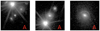 |
Fig. 1 Three grade A candidate lenses found by a visual inspection of 12 086 stamps from the Perseus cluster showing clear lensing features. Each IE-band image is 10′′ × 10′′. Detailed lens models for these candidates are shown in Appendix C of Acevedo Barroso et al. (2025). |
2.3 Construction of the common test set
The ERO data of the Perseus cluster were reserved for testing and comparing the different networks discussed in this work. A team of Euclid Consortium members performed a systematic visual inspection of the 0.7 deg2 Euclid ERO data of the Perseus cluster using both the high-resolution VIS IE-band, and the lower resolution NISP bands (Acevedo Barroso et al. 2025). Every extended source brighter than magnitude 23 in IE was inspected, which amounted to 12 086 stamps of 10′′ × 10′′ with 41 expert human classifiers.
The detailed classification scheme for classifying the sources (see Acevedo Barroso et al. 2025 for details) into one of the following non-overlapping categories, in which A, B, and C are positive grades, whereas X, and I are negative grades, is given as follows:
class A represents definite lenses showing clear lensing features;
class B indicates that lensing features are present, but cannot be confirmed without additional information;
class C denotes that lensing features are present, but can also be explained by other physical phenomena;
class X denotes a definite non-lens;
class I are interesting objects, but are definitely not lensing systems.
The visual inspection resulted in the discovery of three grade A candidates, 13 grade B candidates, and 52 grade C candidates. The 16 combined grade A and grade B candidates were modelled to assess their validity by checking that they were consistent with a single source lensed by a plausible mass distribution, for which five candidates passed this test. The three grade A candidates are shown in Fig. 1.
For this work, however, the decision was made to label the 68 combined grade A, grade B, and grade C candidates as potential lenses. Grade B and C candidates are shown in Fig. A.1. This corresponds to asking each network to select visually plausible lens candidates. Thus, the common test set to evaluate the various networks is composed of the 12 086 stamps, inclusive of the 68 lens candidates being the positives, and the remaining stamps the negatives.
3 Overview of networks
Here, we give an overview of the various networks with their respective training data sets. The networks described in this section represent our current CNN-based detection methods for finding strong lenses in Euclid. In total, 20 networks were used, of which six networks were trained with data from the same simulation sets, created using halo catalogues provided by Euclid Collaboration: Castander et al. (2025), though these training sets differ in size for each network. The remaining networks were trained on their respective training data sets, created specifically for this study using either Galaxy Zoo (Masters 2019, hereafter GZ) and/or the Kilo Degree Survey (KiDS, de Jong et al. 2013) data, which are of different sizes. The training data sets for each network are described in the following subsections. We present the results of evaluating the 20 networks on the common test set in Sect. 5, illustrating which networks are successful lens finders, and which are therefore good candidates for our automated detection pipeline.
3.1 Zoobot
Zoobot (Walmsley et al. 2023) is a Bayesian CNN pre-trained to find morphological features on over 100 M responses by GZ (Masters 2019) volunteers answering a diverse set of classification tasks on over 800 k galaxies from the Sloan Digital Sky Survey (SDSS), Hubble Space Telescope (HST), Hyper Suprime-Cam (HSC), and the Dark Energy Camera Legacy Survey (DECaLS) imaging data (Walmsley et al. 2023).
Zoobot can be trained either from scratch or fine-tuned, a method in which a pre-trained model is adapted to solve a specific task (Walmsley et al. 2022). The latter approach is the most common use of Zoobot, since it takes advantage of the learned representation of galaxy morphology. In this application to Euclid ERO data, we used both approaches. In this work, we take the EfficientNetB0 (Tan & Le 2019) architecture variant of Zoobot, pre-trained on 100 M GZ classifications, and fine-tune it to classify strong lenses in the ERO data set. Here, we fine-tune Zoobot by removing the ‘head’ of the EfficientNetB0 model and fixing the weights of the remaining layers (that is, these layers remain ‘frozen’). We add a new head to the model with outputs appropriate to the new problem of classifying strong lenses; specifically, the binary classification task where the model’s output is a predicted probability that a given input belongs to the positive class (class ‘lens’). The new head is trained to predict outputs for this new problem given the frozen representation and new labels, allowing the new head to benefit from previously learned representations. The new head is composed of two dense layers. The first dense layer has 128 units with dropout probability p = 0.2, and a rectified linear unit (ReLU) activation function. The second dense layer has two units with a softmax activation function.
Fine-tuning a classifier still requires some training examples, though less than training a classifier from scratch (You et al. 2020). A great challenge in astronomy, specifically the research area of strong gravitational lensing, is the lack of sufficiently large labelled data sets to train supervised deep learning models. Similarly to previous studies (e.g. Lanusse et al. 2018; Huertas-Company et al. 2020), the model we describe in this section was trained using simulated images with known labels described in the next section.
3.1.1 Simulated lenses for Zoobot
The data used to train Zoobot for this application were simulated Euclid images from the VIS instrument, created using the Python package Lenzer, specifically designed for this work1. To create the simulations, Lenzer required real galaxy images for the source galaxy to produce the simulated lensed light.
These needed to have at least the same spatial resolution and depth at approximately the same wavelength range as IE-band (Cropper et al. 2016) in order to simulate Euclid-like data. These requirements are fulfilled with the Cosmic Evolution Survey (COSMOS; Scoville et al. 2007) with the Advanced Camera for Surveys (ACS) Wide Field Channel of HST in the F814W filter, with an angular resolution of 0′.′09, and a pixel scale of 0′.′03. The depth and resolution are better than those estimated for Euclid: 24.5 mag at 10σ for Euclid, as opposed to 27.2 mag at 5σ for HST (Euclid Collaboration: Aussel et al. 2024). We note that the wavelength range of the IE-band includes the F814W band of HST; we applied a magnitude restriction of mF814W < 23.5 with a redshift range of 2.5 < z < 5.0, yielding a selection of 36 606 galaxies. We smoothed the selected galaxy images with a kernel given by the difference in HST ACS and VIS point spread function and resampled to give an IE-band pixel scale of 0′.′1. To simulate the lensed light, Lenzer required the Lenstronomy Python package (Birrer & Amara 2018), Skypy (Amara et al. 2021) and Speclite which is part of the Astropy package (Astropy Collaboration 2022). To obtain a list of light profiles for Lenstronomy, we draw a random rotation angle for the galaxy images in our selection and transform the rotation angle and axis ratio into complex ellipticity moduli for the light profile. Redshifts and magnitudes for the lens galaxies were sampled from a distribution of Sloan Lens ACS Survey (SLACS) lens data (Bolton et al. 2008; Shu et al. 2017). From these sampled magnitudes, the velocity dispersions of the lens galaxies, σv, were calculated using the Faber–Jackson relationship (Faber & Jackson 1976), and the Einstein radius of each lensed image, θE, was calculated using
 (1)
where DLS and DS represent the lens-source and the observersource angular diameter distances, respectively, resulting in 0.40 ≤ θE ≤ 2.1. The remaining parameters of the lensed images were randomly sampled using a uniform distribution. Finally, Gaussian noise was added in each pixel to the individual simulated lensed images to reproduce the depth of the IE-band. All simulated lenses represented strongly lensed systems. The simulated lens images were randomly added to sources extracted from two other ERO fields, NGC6397 and NGC6822, with magnitudes IE < 23. These two ERO fields do not overlap the Perseus cluster. A total of 50 000 simulated lensed images were produced. The training set was also composed of 50 000 negatives from real Euclid data. The negatives were sources extracted from the two ERO fields mentioned above, which were not used in creating the simulated lensed images.
(1)
where DLS and DS represent the lens-source and the observersource angular diameter distances, respectively, resulting in 0.40 ≤ θE ≤ 2.1. The remaining parameters of the lensed images were randomly sampled using a uniform distribution. Finally, Gaussian noise was added in each pixel to the individual simulated lensed images to reproduce the depth of the IE-band. All simulated lenses represented strongly lensed systems. The simulated lens images were randomly added to sources extracted from two other ERO fields, NGC6397 and NGC6822, with magnitudes IE < 23. These two ERO fields do not overlap the Perseus cluster. A total of 50 000 simulated lensed images were produced. The training set was also composed of 50 000 negatives from real Euclid data. The negatives were sources extracted from the two ERO fields mentioned above, which were not used in creating the simulated lensed images.
Diversity of gravitational lensing systems is important to consider, and simulations of gravitational lenses using different methods can provide a range of different lensing configurations. The second data set we used to train from scratch and fine-tune Zoobot were lens simulations with known labels, created in the same manner as above, using an elliptical Sérsic light profile, and SIE mass model for the lens galaxy, but with HST Ultra Deep Field (UDF) sources as source galaxies. Likewise, these simulations represented strongly lensed systems only. However, the simulated lensed images added to the source galaxies were produced in a different way. For a more detailed description of the simulation set, see Sect. 3 of Metcalf et al. (2019).
3.1.2 Experiments and training procedure
We thus trained the EfficientNetB0 model with four different approaches and present a comparison of results in Sect. 5. In two of the approaches, we trained the EfficientNetB0 model from scratch on two sets of simulated gravitational lenses, Lenzer and those described in Metcalf et al. (2019). We will hereafter denote these networks with E1 and E2, respectively. For the remaining two approaches, we took the pre-trained network on the GZ classifications and fine-tune it with the same two simulation sets as before. We denote the fine-tuned networks as Zoobot1 and Zoobot2, respectively.
These four networks were trained in the same fashion. The images were resized to 300 × 300 pixels and normalised to have pixel values between 0 and 1. We trained each network up to 100 epochs with train/validation/test sets split sizes of 80%/10%/10%, respectively. The test sets we describe here are not used for training, and were only used to evaluate the performance of each network on the two simulation sets. We used the binary-cross entropy loss and the adaptive moment estimation optimiser (Adam; Kingma & Ba 2015) with a learning rate of 10−4. Adam introduces an adaptive learning rate over standard optimisation methods such as stochastic gradient descent (SGD). We applied a softmax activation to each network’s output to obtain a predicted probability of the positive class (class ‘lens’). We set a probability threshold of pTHRESH = 0.5 for all networks for a given input to belong to the positive class, such that an image will be classified as a lens if the prediction of the network for the positive class is above pTHRESH. This is set by default in the Zoobot documentation but can be adapted (Walmsley et al. 2022), although we kept the default probability threshold for this work. For each network, we saved the best weights which correspond to the epoch with the minimum validation loss, and we used early stopping to end training if the validation loss ceased to converge, thereby ending further training after epoch 92 for Zoobot1. The remaining three networks were trained for 100 epochs. All Zoobot models were adapted to take the 10′′ × 10′′ images in the common test set as input.
3.2 Naberrie and Mask R-CNNs
The five networks we discuss in this section are Naberrie, based on a U-Net architecture (Ronneberger et al. 2015), and four Mask R-CNNs, or Mask Region-based CNNs, (He et al. 2017), namely MRC-95, MRC-99, MRC-995, and MRC-3. U-Net is a CNN originally designed for image segmentation (Ronneberger et al. 2015), consisting of a contracting path and expansive path which are approximately symmetrical, giving the model its U-shape. The difference between U-Net and a generic CNN is the use of up-sampling whereby the pooling layers of a generic CNN are replaced by up-convolution layers, thus increasing the resolution of the output. Similar to U-Net, the Mask R-CNNs are designed for image segmentation but they also combine this with object detection. The Mask R-CNNs are able to perform pixel-wise segmentation using the ‘Mask’ head which generates segmentation masks for each object detected (He et al. 2017).
The U-Net Naberrie is made up of three separate parts: the encoder, the decoder, and the classifier. Figure 2 shows its architecture. Naberrie takes an IE-band image of 200 × 200 pixels, corresponding to 20′′ × 20′′ with an IE-band pixel scale of 0′.′1. The encoder section is made of several convolutional layers with max-pooling and dropout applied. This produces a bottleneck that is a dimension-reduced representation of the input data. The decoder section is trained to take the bottleneck data as input and to produce an image as an output. The target for the decoder is to produce an image showing only the light from the lensed galaxy in the input image. The classifier also takes the bottleneck data as input; the goal of the classifier is to classify the input image as either a lens (1) or a non-lens (0). The classifier is made up of fully-connected layers and ReLU activation functions.
The Mask R-CNNs all had the same ResNet-50 architecture (He et al. 2016) where the default final layer for each model was replaced with a sigmoid activation to output a probability of an image belonging to class lens (1) or non-lens (0), with the rest of the model weights frozen. The main difference between the variations of the Mask R-CNNs was the threshold of the masking based on percentiles of the images (0.95, 0.99, and 0.995, respectively); MRC-3 also had a mask threshold of 0.995. For example, MRC-995 uses regions of the images above the 99.5th percentile. For more information, we refer the reader to Wilde (2023).
The simulated data used to train the models Naberrie, MRC-95, MRC-99, MRC-995, and MRC-3 were created using Lenstronomy (Birrer & Amara 2018) with lens parameters taken from Metcalf et al. (2019). The aims of these simulations were to train models that could be more interpretable than the standard CNN by providing a location for lensing features through building interpretability into the model, since the Mask R-CNNs use object detection methods, rather than interpretability techniques being used post-training (Jacobs et al. 2022; Wilde et al. 2022). The redshifts and magnitudes were sampled from the second strong gravitational lens finding challenge training data set (Metcalf et al. 2019), which involve similar but not identical lens parameters as those used in the simulations in Sect. 3.1 for networks Zoobot2 and E2. From this, the velocity dispersion was determined (Faber & Jackson 1976) and the Einstein radius calculated to be in agreement with Einstein radii reported in Sloan Lens ACS survey data (SLACS Bolton et al. 2008; Auger et al. 2009; Newton et al. 2011; Shu et al. 2017; Denzel et al. 2021). The simulations used an elliptical Sérsic light profile and an SIE mass model. Other galaxy parameters were sampled from a uniform sampling of SLACS survey data. The training set contained a total of 10 000 cutouts in the form of the strongly lensed simulations described above. Naberrie required a target of the lens light for the decoder, and the Mask region-based CNNs (Mask R-CNNs) required a mask for each galaxy. The full details of this, and the validation and test sets used, can be found in Wilde (2023).
Naberrie was trained in two stages both using 10 000 IEband 20′′ × 20′′ cutouts for 50 epochs with a learning rate of 3 × 10⁻⁴, and a batch size of 10. In the first stage, we trained the encoder and the decoder. Once these had been trained, the best weights from the epoch with the lowest validation loss are saved, and loaded into Naberrie. In the second stage, the training is done after freezing the encoder weights to the best weights from the previous stage, and replacing the decoder by the classifier. Finally, all three sections of Naberrie were assembled to form the final trained model. The Mask R-CNNs were trained using 10 000 IE-band 20′′ × 20′′ cutouts with a learning rate of 3 × 10⁻⁴, and a batch size of 10, for 50 epochs (for MRC-95, MRC-95, MRC-995) and 100 epochs (for MRC-3). The Mask R-CNN outputs a probability for each class, a mask for the detection, and a bounding box for the detection. The classifiers described in this section were trained with the binary-cross entropy loss optimised by the Adam optimisation method (Kingma & Ba 2015). The images within the common test set were resampled/resized to 200 × 200 pixels, corresponding to 0′.′1/pixel, to be taken as input by Naberrie and the Mask-RCNNs.
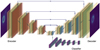 |
Fig. 2 Layers that construct the U-Net Naberrie including an encoder, a decoder, and a classifier. The arrows represent skip connections, connecting extracted features from the encoder section to the decoder section. |
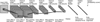 |
Fig. 3 Scheme of the architecture of the 4-layer CNN. The 4-layer CNN takes an 100 × 100 pixel IE-band image as input, and extracts features through blocks of convolution layers and max-pooling layers, with ReLU activation functions. The final fully-connected layer uses a sigmoid activation to produce a probability score as output, with 1 belonging to class lens. |
3.3 NG (Napoli-Groningen) and ResNet-18
The Napoli-Groningen network, NG, is a CNN with an architecture based on the model described in Petrillo et al. (2019a), employing a ResNet-18 architecture (He et al. 2016). The network takes an input in the form of a 200 × 200 pixel image, corresponding to 20′′ × 20′′ for an IE-band pixel scale of 0′.′1, and outputs a number between 0 and 1, which represents the probability of the image being a candidate lens. The training data consisted of approximately 6000 strong lenses, and 12 000 non-lenses. The lenses were created from r-band KiDS luminous red galaxies (LRGs) by super-imposing 106 simulated lensed objects. The simulated lensing features were mainly rings, arcs, and quads. The gravitational lens mass distribution adopted for the simulations was assumed to be that of an SIE mass model, perturbed by additional Gaussian random field fluctuations and external shear. An elliptical Sérsic brightness profile was used to represent the lensed sources, to which several small internal structures were added (such as star-formation regions), described by circular Sérsic profiles. The non-lenses in the training set are galaxies from KiDS composed of normal LRGs without lensing features, randomly selected galaxies from the survey with r < 21 magnitude, mergers, ring galaxies, and a sample of galaxies that were visually classified as spirals from a GZ project (Willett et al. 2013). NG was trained with the binary-cross entropy loss optimised by the Adam optimisation method (Kingma & Ba 2015) with a learning rate of 4 × 10⁻⁴ for 100 epochs, where, similar to Sect. 3.2, the common test set images were resized to the required 200 × 200 input size of NG. For further details see Petrillo et al. (2019a,b).
Additionally, the same ResNet architecture was trained on a different set of lens simulations described in Sect. 3 of Metcalf et al. (2019), namely ResNet-18, with the final three layers replaced by fully-connected dense layers followed by a sigmoid activation. We trained the network on 80 000 simulated strong gravitational lenses, and corresponding non-lenses, of size 10′′ × 10′′, in the same manner for NG as described above.
3.4 4-layer CNN
We test the performance of a shallow 4-layer CNN in identifying strong lens candidates in the ERO data of the Perseus cluster. The CNN architecture used, shown in Fig. 3, was an adaptation of the network developed for the morphological classification of galaxies in Domínguez Sánchez et al. (2018), and had already been tested with Euclid-like simulations (Manjón-García 2021). The network had four convolutional layers of different spacings (6×6, 5×5, 2×2, and 3×3, respectively), and two fully-connected layers. ReLU activation functions were applied after every convolutional layer, and a 2 × 2 max-pooling was applied after the second and third convolutional layers.
The training of the network was carried out following a supervised learning approach with labelled 10′′ × 10′′ IE-band images. The training data set for the network was strong lens simulations created by Metcalf et al. (2019), which include companions that are also lensed. It consisted of 60 000 images split into 90% for training and 10% for validation, with a balanced distribution of strong lenses and non-lenses. The lens simulations assumed an elliptical Sérsic light profile perturbed by an SIE mass model. We investigated training under different conditions (simulation data sets used, training set sizes, data pre-processing, small changes in the architecture and learning parameters) in order to achieve both the lowest loss and false positive rate, whilst maintaining a high true positive recovery. The best network, however, yielded many false positives when tested on the Perseus cluster, which will be described in detail in Sect. 5. The network read IE-band images of 100 × 100 pixels, corresponding to 10′′ × 10′′ in IE-band, in which the fluxes were normalised to the maximum value. In the learning process, we used a binary cross-entropy loss function optimised by the Adam stochastic optimisation method (Kingma & Ba 2015), with a learning rate of 10−3. The model was trained for 20 epochs, using a batch size of 24. In order to prevent over-fitting, several data augmentation techniques were performed during training, allowing the images to be zoomed in and out (0.75 to 1.3 times the original size), rotated, and flipped and shifted both vertically and horizontally. Finally, in the last fully-connected layer, a sigmoid activation function was used to turn the output scores into probabilities of being a lens distributed between 0 and 1, with 1 denoting the class ‘lens’.
3.5 Denselens and U-Denselens
Denselens (Nagam et al. 2023) is an ensemble of classification and regression networks to classify and rank strong lenses. Denselens is constructed with a densely connected convolutional network (DenseNets, Huang et al. 2017) architecture as a backbone in which the layers are connected in a feed-forward manner. Here, we describe the Denselens network and an adaptation of this network which we call U-Denselens, where an additional U-Net is added to the original Denselens architecture. We take the frozen weights of the pre-trained Denselens network for this application.
The Denselens network includes an ensemble of four classification prediction networks in which each network predicts an output value in the range [0, 1]. The mean of the output predictions from the four networks, Pmean, were calculated and the candidates whose predictions fall above a threshold (pTHRESH) were classified as strong lens candidates, while the rest were classified as non-lenses. We set the pTHRESH value to be 0.23 for this application to find strong lenses, since this value of pTHRESH maintained a true positive recovery of 50%. The candidates that were classified as lenses were then passed to the second set of ensemble networks comprising four CNNs, trained on the Information Content (IC) value of mock simulated lenses. The IC values used for training lenses were calculated based on Eq. (2):
![Mathematical equation: $\textrm{IC} = \left [\frac{ A_{\textrm{src,}2\sigma} }{A_\sfont{PSF}} \right] R,$](/articles/aa/full_html/2025/04/aa53152-24/aa53152-24-eq2.png) (2)
where Asrc,2σ is the total area of the lensed images above a brightness threshold in terms of noise level of 2 σ. The area of the PSF (APSF) is defined as the square of Full Width Half Maximum (FWHM) and R = (θE/Reff) is the ratio of the Einstein radius (θE) to the effective source radius (Reff). In practice, IC can be used as an effective metric to rank-order lenses that are easy to recognise for a human or CNN classifier.
(2)
where Asrc,2σ is the total area of the lensed images above a brightness threshold in terms of noise level of 2 σ. The area of the PSF (APSF) is defined as the square of Full Width Half Maximum (FWHM) and R = (θE/Reff) is the ratio of the Einstein radius (θE) to the effective source radius (Reff). In practice, IC can be used as an effective metric to rank-order lenses that are easy to recognise for a human or CNN classifier.
In addition to this, in our second network, U-Denselens (Nagam et al. 2024), we included a U-Net (Ronneberger et al. 2015) at the end of the Denselens pipeline, to further improve the accuracy in detecting strong lenses and reducing the false positive rate. The U-Net network was trained by designating all source pixels to a value of 1 and all other pixels to 0. The output of the U-Net corresponds to a map of 101 × 101 pixels. Each pixel in the output map varies in the range [0, 1] since a sigmoid function has been used as an activation function in the final layer. Using the information from the source pixels, we defined a metric, ns, which is calculated by the number of source pixels above a segmentation threshold, S THRESH. This segmentation threshold represents the pixels that are considered to belong to the source by U-Net, and which take values between 0 and 1 after re-normalising the images. Setting the threshold too low would result in selecting pixels for which the U-Net lacks confidence. Conversely, a high threshold could lead to a multitude of candidates with minimal pixels in the segmentation output. We set the S THRESH for Denselens and U-Denselens to a small value of 0.01, and we set pTHRESH = 0.18 for U-Denselens for this application to the Perseus cluster. For more information, we refer the reader to Nagam et al. (2024). The candidates that passed the pTHRESH and have ns > 0 were selected as lens candidates. The candidates that were rejected with ns = 0, were only retained if they have IC ? 88. This step of retaining based on the IC was done to reduce the rejection bias of the segmentation network since the network was not trained with all possible combinations of extremely diverse lens samples present.
KiDS data were used to create the simulated data to train Denselens and U-Denselens. The training data set comprised 10 000 samples, balanced between 5000 mock strong lenses and 5000 non-lenses. The source galaxies were modelled by sampling parameters from a Sérsic profile, such as the effective radius Reff, and the Sérsic index n. The lens galaxies were modelled with an SIE mass distribution and an elliptical Sérsic light profile. For more information on the lensing simulations used to train Denselens, see Nagam et al. (2023, 2024). All mock lenses represented strongly lensed systems. The mock lenses were randomly painted over the roughly 5000 selected LRGs from the KiDS data set. The negatives comprised 5000 galaxies, including random galaxies, sources that have been wrongly identified as mock lenses in previous tests, and also visually classified spiral galaxies from a GZ project. Each simulated mock lens and nonlens corresponded to an area of 20′′ × 20′′. The images within the common test set were resized on input to accommodate this. The training strategy of Denselens and U-Denselens, and more information regarding the simulations used for training, and validation and test sets, are explained in detail in Nagam et al. (2023, 2024), respectively.
3.6 LensCLR
Here, we explore the application of semi-supervised learning for detecting lens candidates, as it offers a compelling advantage over fully-supervised learning by leveraging both labelled and unlabelled data to enhance model performance (e.g., Stein et al. 2022; Huertas-Company et al. 2023). This approach addresses the challenge of acquiring large labelled data sets, which are often costly and time-consuming to obtain. Semi-supervised learning involves two training steps. First, the network is trained using unlabelled images to learn the underlying data patterns and structures in a self-supervised manner via contrastive learning. The aim of this process is to cluster similar images together in the latent space while pushing dis-similar images apart (Chen et al. 2020a). Then, the pre-trained network is fine-tuned for the classification task using a small number of labelled images. This strategy not only reduces labelling costs but also improves generalisation and robustness, since the models can capture a wider variety of patterns from diverse unlabelled data (Chen et al. 2020b; He et al. 2020).
Our model follows the simple framework for contrastive learning of visual representations proposed by Chen et al. (2020a). LensCLR comprised three main components: augmentation, backbone, and projector modules. For the backbone, we used EfficientNetV2B0 to transform each input image into a lower-dimensional representation, yielding a 1280-dimensional vector as output (Tan & Le 2021; Andika et al. 2023b). Following that, we attached two dense layers, each with 128 neurons, as the projector; collectively, the backbone and the projector form the encoder. Finally, the encoder learns meaningful representations by employing a contrastive loss function, associating augmented views of the same image as similar and views of different images as dissimilar (van den Oord et al. 2018).
The first phase of the training, also called pre-training or the pretext task of LensCLR, via contrastive learning, was done by using an unlabelled data set containing around 500 000 sources in the Perseus cluster. This data set, called DS1, included real galaxies, stars, quasars, photometric artefacts, and other features observed in IE images. In the training loop, batches of 512 images of 150 × 150 pixels were randomly selected from DS1 as inputs, and their fluxes were scaled to be between 0 and 1 using min-max normalisation. These images were then passed through the augmentation module, which transformed the inputs with random flips, ±π/2 rotations, and 5-pixel shifts, as well as a centre-crop to trim them to 96 × 96 pixels.
We note that augmenting sample xq produces a pair of views marked as positive (xq, xk+) if they originate from transformations of the same source. In other words, there is a (positive) similarity, since the pair of views originate from the same source with the difference being that one is augmented, and negative (xq, xk−) otherwise, since the pair of views originate from different sources and are thus dissimilar (e.g. Hayat et al. 2021). Next, these images were processed by the encoder, where the output is projected into a 128-dimensional vector: z = encoder(x). Model optimisation was then performed, starting with an initial learning rate of 10−3, by minimising the contrastive loss given by:
![Mathematical equation: $L_{q, k^+, \{k^-\}}= -\ln \left\{ \frac{ \exp[ \mathrm{sim}(\vec{z}_q , \vec{z}_{k^+})] } { \exp[ \mathrm{sim}(\vec{z}_q , \vec{z}_{k^+})] + \sum_{k^-} \exp[ \mathrm{sim} (\vec{z}_q , \vec{z}_{k^-})] }\right\}.$](/articles/aa/full_html/2025/04/aa53152-24/aa53152-24-eq3.png) (3)
(3)
We note that sim(a, b) = a · b/(τ |a| |b|) represents the cosine similarity between vectors a and b, scaled by a configurable ‘temperature’ parameter τ. This loss function, also known as information noise contrastive estimation (InfoNCE; van den Oord et al. 2018), was optimised to ensure that similar pairs (positive pairs) exhibit high similarity, whereas dissimilar pairs (negative pairs) display low similarity.
In the second phase of training, we fine-tuned LensCLR using a supervised learning approach with labelled images. The labelled data set, referred to as DS2, was derived from the strong lens simulation created by Metcalf et al. (2019), containing 50 000 strong lens and 50 000 non-lens systems of 10′′ × 10′′ in IE-band, identical to other training sets used in this work. The simulations assumed an elliptical Sérsic light profile and an SIE mass model of the lens galaxy, and a Sérsic profile for the source galaxy. For a more detailed description of the simulation set, see Sect. 3 of Metcalf et al. (2019). We split DS2 into training, validation, and test data sets with a ratio of 70%:20%:10%. After that, a modification needed to be applied to the encoder by removing the projector and replacing it with a single dense layer consisting of one neuron with a sigmoid activation function. This single dense layer later becomes the classification layer. During fine-tuning, all weights in the pre-trained encoder were frozen, and only the classification layer was trained. The objective was to differentiate between lenses and non-lenses using a binary cross-entropy loss function optimised with the Adam optimiser (Kingma & Ba 2015), and initial learning rate of 10−4.
During the training loop, we implemented a scheduler that reduces the learning rate by a factor of 0.2 if model performance did not improve over five consecutive epochs (e.g., Andika et al. 2023a). Additionally, early stopping was used if the loss did not decrease by at least 10−4 for 10 consecutive epochs. After 200 epochs, our model converged, and the optimised parameters were saved.
3.7 VGG, GNet, and ResNext
In Euclid Collaboration: Leuzzi et al. (2024), we applied three network architectures to find lenses in simulated Euclid-like images: a VGG-like network, a GNet which includes an inception module, and a residual network ResNext. We now apply all the architectures to the ERO Perseus cluster data set.
While we refer the reader to Euclid Collaboration: Leuzzi et al. (2024) for a detailed description of the architectures, we summarise their main characteristics here. The VGG-like network (inspired by Simonyan & Zisserman 2015) has ten convolutional layers alternating with five max-pooling layers, followed by two fully-connected layers. The main building block of GNet is the inception module introduced by Szegedy et al. (2015, 2016). The inception module is implemented as a series of convolutions of different sizes (1 × 1, 3 × 3, 5 × 5) run in parallel on the same image to extract features on different scales simultaneously. Our implementation of this architecture starts with two convolutional layers alternating with two max-pooling layers. After this, there is a sequence of seven inception modules, the fifth of which is connected to an additional classifier. When computing the loss function during training, the input of the fifth and of the final output layers are combined, with different weights (0.3 and 1.0, respectively). The ResNext is based on the concept of residual learning introduced by He et al. (2016) and Xie et al. (2016), and is implemented in such a way that every building block of the architecture does not have to infer the full mapping between the input and output, but only the residual mapping. This is implemented through shortcut connections (He et al. 2016). Our version of this architecture comprised two convolutional layers and four residual blocks alternating with two max-pooling layers. The final layer of all networks used the sigmoid function to provide a value in the range 0 to 1, used for the classification of the image as a lens or non-lens as a probability score, given the desired threshold (we set pTHRESH = 0.5).
We trained the networks with 100 000 Euclid-like mock images, created by Metcalf et al. (2019), using 50 000 strong lens images and 50 000 non-lens images, all of which were 10′′ × 10′′ in IE-band. The simulations were based on the halo catalogues provided by the Flagship simulation (Euclid Collaboration: Castander et al. 2025), which used an elliptical Sérsic light profile and an SIE mass model for the lens galaxy, and a Sérsic profile for the source galaxy. All networks were trained for 100 epochs, with an initial learning rate of 10−4, adjusted during training to improve convergence, depending on the trend of the validation loss function over time. We used the Adam optimiser (Kingma & Ba 2015) and the binary cross-entropy loss. The pre-processing of the images and training procedure are further detailed in Sect. 4 of Euclid Collaboration: Leuzzi et al. (2024).
3.8 Consensus-Based Ensemble Network (CBEN)
The Consensus-Based Ensemble Network (CBEN) leverages the complementary strengths of seven CNNs: ResNet-18 (He et al. 2016); EfficientNetB0 (Tan & Le 2019); EfficientNetV2 (Tan & Le 2021); GhostNet (Tan & Le 2021); MobileNetV3 (Howard et al. 2019); ReGNet (Radosavovic et al. 2020); and Squeeze-and-Excitation ResNet (SE-ResNet, Hu et al. 2018). Each of these networks has been independently trained to classify lenses. By incorporating diverse architectures within the ensemble, CBEN benefits from the varied feature extraction capabilities and decision-making heuristics of the individual models.
The standout feature of CBEN is its decision-making process, which relies on a unanimous voting mechanism, where a data sample is classified as belonging to the positive class only if all seven models independently agree on this prediction, such that the prediction, p > β, for 0 < β < 1. In that case, the model score is taken as the minimum of all model scores. Conversely, if there is any disagreement among the models, the sample is classified as belonging to the negative class, with the model score taken as the maximum of all model scores. This criterion ensures a high level of confidence and reduces the likelihood of false positives, which is critical in lens identification where the cost of a false positive is high. We investigated the performance of CBEN with β = 0.3 and β = 0.0001, hereafter CBEN-0.3 and CBEN-0.0001, respectively.
All networks were trained on mock images resembling those of Euclid IE-band, simulated in accordance with the methods described in Metcalf et al. (2019), incorporating enhanced noise and PSF modelling, using an elliptical Sérsic light profile and an SIE mass profile for the lens galaxy, and a Sérsic profile for the source galaxy. The training data set consisted of 80 000 images, split evenly with 40 000 strong lenses and 40 000 nonlenses, with an additional 10 000 samples used for validation, and another 10 000 for testing. The images were pre-processed by cropping them to dimensions of 96 × 96 pixels and normalising their pixel values to a range of [0, 1]. During training, we employed the Adam optimiser (Kingma & Ba 2015) with a learning rate of 10−4, and binary cross-entropy loss. After 100 epochs, the models with the lowest validation error were saved and tested on the common test set. The images in the common test set were pre-processed in the same way to dimensions of 96 × 96 pixels with 0′.′1/pixel.
4 Metrics used for analysis
The performance of a network can be assessed in many ways, however we focus both on the number of true positives (TPs) recovered, the and false positives (FPs) found from the common test set of 12 086 stamps from the Perseus cluster. We first define the true positive rate and false positive rate metrics (hereafter TPR and FPR, respectively), which are used to visualise a network’s performance using a Receiver Operating Characteristic curve (ROC). Then, using the ROC curve, we calculate another metric known as the Area Under the ROC curve (AUROC). Here, we give an overview of these metrics which we use to evaluate the performance of the various networks, in addition to introducing the importance of interpreting the false positives.
4.1 TPR and FPR
In our context, a true positive refers to a candidate lens correctly identified as belonging to the positive class (class ‘lens’), and a false positive represents a non-lens falsely identified as belonging to the positive class. We use the following definitions of true positive rate (TPR, also known as recall or sensitivity) and false positive rate (FPR, also known as contamination or specificity) at a given threshold:
 (4)
where NTP is the number of true positive (TP) stamps that are correctly predicted, NTN is the number of true negative (TN) stamps that are correctly predicted, and NFN indicates the number of stamps that belong to the positive group but are falsely classified as negative (false negatives, or FN). Finally, NFP represents the number of stamps that belong to the negative group but are false positives (FP). For our application to the 12 086 stamps from the Perseus cluster, TPR represents to proportion of grade A, grade B, and grade C lens candidates correctly identified, and FPR represents the proportion of stamps incorrectly classified as a lens.
(4)
where NTP is the number of true positive (TP) stamps that are correctly predicted, NTN is the number of true negative (TN) stamps that are correctly predicted, and NFN indicates the number of stamps that belong to the positive group but are falsely classified as negative (false negatives, or FN). Finally, NFP represents the number of stamps that belong to the negative group but are false positives (FP). For our application to the 12 086 stamps from the Perseus cluster, TPR represents to proportion of grade A, grade B, and grade C lens candidates correctly identified, and FPR represents the proportion of stamps incorrectly classified as a lens.
4.2 ROC
We can visualise a network’s classification performance at every possible threshold using a Receiver Operating Characteristic curve (ROC) which shows the TPR vs FPR, that were defined in the previous section. A binary classifier generally gives a probability of a candidate being a lens, pLENS, in which case a threshold is set, namely pTHRESH, and everything with pLENS > pTHRESH is classified as a lens. At pLENS = 0, all of the cases are classified as non-lenses and so TPR = FPR = 0, and at pLENS = 1, all of the cases are classified as lenses so TPR = FPR = 1. These points are always added to the ROC curve. If the classifier made random guesses then the ratio of lenses to non-lenses would be the same as the ratio of the number of stamps classified as lenses to the number of stamps classified as non-lenses and so TPR = FPR. For our application to the Perseus cluster, the best classifier will have a small FPR and a large TPR, and so the further away from this diagonal line it will be.
4.3 AUROC score
From the ROC curve described in the previous section, we can calculate the Area Under the ROC (AUROC) score, another metric which is widely used in other studies (Metcalf et al. 2019). A large AUROC score means that many true positives can be recovered at low false positive rates. A small AUROC score means that high false positive rates are required to achieve high true positive recovery. AUROC ranges between 0 and 1, where a value of AUROC close to 0.5, and below, show a poor classification, with an AUROC score of 0 meaning that the classifier is always wrong in its classification. An AUROC score of 1 represents a perfect classifier (for more information about ROC and AUROC metrics see Teimoorinia et al. 2016 and references therein). Our best classifier will have a high AUROC score.
4.4 Interpreting false positives
In addition to the important metrics defined above, we will also give an interpretation of the false positives in the results. Comparing the false positive rate, and the number of false positives (or the contamination), of each network allows us to access the classification performance when the networks, previously trained on simulations, are applied to real data. The networks with a low false positive rate have a low contamination (meaning they find few false positives). These networks therefore have a lower contamination rate, defined by NFP/NTP, and produce a more pure sample of lenses. The contamination rate is an important metric to consider, since networks with large contamination rates could find large numbers of false positives if applied to future Euclid observations, beyond which a visual inspection is infeasible.
Additionally, an investigation into the most frequent galaxy morphologies contaminating the classification result across all networks indicates which features the networks are responding to, and allows us to proceed by introducing these negatives in future training of the networks.
5 Results
Here, we attempt a systematic comparison of network performance in preparation for CNN-based detection pipelines for the VIS images of the ERO data of the Perseus cluster using the metrics defined in Sect. 4 to compute the ROC of each network. We compute the AUROC score for each network and compare the FPR and TPR of the networks. Additionally, we compare the lens misclassifications which are common to the majority of our networks.
5.1 ROC and AUROC
In total, 20 networks were trained with their respective training sets and evaluated on the common test set of 12 086 real ERO stamps from the Perseus cluster that were visually inspected. Here, we characterise and compare the performance of the various networks in terms of the ROC and AUROC score as defined in the previous section.
Figure 4 shows the ROC curves for all networks evaluated on the common test set. The random classifier (orange dotted line) serves as a reference. The ROC curves represent the proportion of the 68 lens candidates from the expert visual inspection correctly identified as lens candidates against the proportion of non-lenses in the expert visual inspection sample falsely identified as lens candidates by each network. To quantify the performance of each network, we compute the AUROC score. A perfect binary classifier would have an AUROC score of 1.0, meaning that the classifier can distinguish between all positive and negative class points.
Figure 4a shows the performance of the four EfficientNetB0 networks, of which two are pre-trained on GZ classifications and fine-tuned on the separate simulation sets described in Sect. 3.1, namely Zoobot1 and Zoobot2, shown by the red and blue lines, respectively. The remaining two networks are trained from scratch on the same two separate simulation sets, E1 and E2, shown by the green and magenta lines, respectively. The fine-tuned EfficientNetB0 networks, namely Zoobot1 and Zoobot2, appear to be effective classifiers and are more confident in ranking a candidate lens higher than a non-lens than E1 and E2. The best performing network out of the EfficientNetB0 networks is Zoobot1, which achieves an AUROC score of 0.91. The fact that Zoobot1 is confident at identifying lens candidates is most likely attributed to its pre-training on 800 k galaxy images with over 100 M volunteer responses and fine-tuning on training data sets given by Lenzer, which incorporates real Euclid images into the strong lens simulations, such that subtle effects from noise, for instance, was included in Zoobot1’s training. However, the fine-tuned EfficientNetB0 network trained on a different set of simulations, Zoobot2, only achieves an AUROC score of 0.68. This reinforces the fact that the training sample used to fine-tune the networks has a significant impact on the performance. This becomes evident when we compare the results of the Zoobot networks trained from scratch without the learned representation of galaxy morphology from GZ on the same simulation sets, namely E1 and E2, which are worse at correctly classifying the lens candidates.
Figure 4b shows the ROC curves for the networks described in Sect. 3.2, which are trained on similar simulation sets to Zoobot2 and E2. These networks do not appear to be strong classifiers. The best-performing model in Fig. 4b is MRC-3 with an AUROC score of 0.66. Although MRC-3 achieves a relatively low AUROC score, it out-performs Naberrie, which achieves an AUROC score of 0.45 and performs worse than a classifier that ranks lenses and non-lenses at random. Thus, it is possible that the network architecture is an important factor in performance, in addition to the training sample, with MRC-3’s ResNet-50 architecture out-performing the segmentation approach of U-Net in Naberrie. MRC-3 performs similarly to the pre-trained Zoobot2 network which is fine-tuned on a similar data set. It is worth noting that U-Net is a more complex architecture than the Mask R-CNN architecture, and thus the performance of Naberrie might improve with a larger training data set.
Figure 4c presents the classifier performance of the two ResNet-based architectures, NG and ResNet-18 described in Sect. 3.3 , shown in red and blue, respectively, compared to the 4-layer CNN, described in Sect. 3.4, shown in green. The performance of these three networks is relatively similar, yet better than a random classifier, with the 4-layer CNN slightly outperforming the ResNet-based networks, with an AUROC score of 0.77 as opposed to 0.71 and 0.65 for NG and ResNet-18, respectively.
The networks with a commensurate classifier performance to that of Zoobot1 are Denselens, and LensCLR, shown in Fig. 4d, with AUROC scores of 0.83 and 0.87, shown in red and green, respectively. Like Zoobot1, these networks are more confident in identifying lens candidates and ranking those higher than its non-lens counterpart. LensCLR uses a semi-supervised approach, as opposed to the fully-supervised training of all other networks presented in this work. This has proven beneficial in the network’s performance since it has been trained with and without labelled data. Additionally, Denselens uses an ensemble of networks which leads to the benefit of the capability to rankorder candidate lenses to reduce the stochastic nature of trained parameters in CNNs. As a result, Denselens benefits from its sophisticated architecture, achieving a higher AUROC score than NG, mentioned above, which is trained on similar ground-based r-band data from KiDS. However, with the addition of the U- Net, U-Denselens does not outperform its Denselens base architecture, with an AUROC score of 0.73, similar to that of NG.
The networks described in Sect. 3.7, however, perform no better than a random classifier, shown in Fig. 4e. The three networks, VGG, ResNext and GNet, are unable to classify candidate lenses higher than the non-lenses in the common test set, with ResNext achieving the highest AUROC score of 0.54, while VGG and GNet give AUROC scores of 0.51 and 0.53, respectively. We recapitulate that the training sample for a network has a significant impact in the network’s performance, yet the network architecture, training set size, and the complexity of the network can also play a crucial role. A more in-depth analysis would need to be taken to investigate the performance of these networks
Finally, Fig. 4f shows the ROC curves for CBEN evaluated at two voting values β, namely CBEN-0.3 and CBEN-0.0001, shown in red and blue, respectively. Although CBEN-0.0001 performs better than its counterpart CBEN-0.3, its increased performance is not large, achieving an AUROC of 0.76 in contrast to 0.72 for CBEN-0.3. Although both CBEN networks perform better than other networks in this study, their overall performance is only at most 76% confident at classifying a candidate lens higher than a non-lens. Though using a different training sample could increase the classifier performance of CBEN, despite the ensemble of seven CNNs assembling its sophisticated architecture, it is not as confident at classifying candidate lenses as other networks in this study of the Perseus cluster. Therefore, Zoobot1, Denselens, 4-layer CNN, and LensCLR are the best overall classifiers for this application.
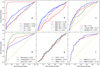 |
Fig. 4 ROC curves for the networks described in Section 3. Performance of the Zoobot networks are shown in panel (a), Naberrie and MRC networks are shown in (b), NG, 4-layer CNN, and ResNet-18 are shown in (c), and Denselens and LencCLR are shown in (d). The performance of the networks described in Sect. 3.7 are shown in (e), and (f) shows the CBEN networks at two voting values β = 0.3 and β = 0.0001, respectively. The orange diagonal line marked represents the expected performance of an entirely random classifier. The values in the legend of each subplot represent the true positive recovery for each network. Higher performance is represented in general by curves approaching the top-left corner of the plots. |
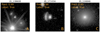 |
Fig. 5 Examples of correctly identified candidate lenses (or true positives) by Zoobot1 in the IE-band. The grade of each candidate is shown at the bottom of each subplot. Each subplot contains the predicted score, pLENS for that candidate along with the true class (with True belonging to class ‘lens’). Each candidate lens image is 10′′ × 10′′. |
5.2 TPR and FPR
The TPR and FPR, described in Sect. 4.1, are of importance in lens finding, since the number of true positives is generally low due to the fact that strong lensing affects ≈1 in 10 000 galaxies. Meanwhile, the cost of a false positive is high. Ideally, the optimal network will have a high TPR and a low FPR, but often there is a trade-off between the two quantities, so we want a network that strikes a balance between the TPR and FPR, thus finding the majority, if not all, of the lens candidates in our common test set with few false positives. In this section, we compare the TPR and FPR of our best performing networks only, but the results for all networks are presented in Table 1.
LensCLR and Zoobot1 have the highest AUC score of all networks, however, their performance is different with respect to TPR and FPR. Although LensCLR has the highest TPR of all networks finding 62/68 lens candidates with a recall score of 94%, and recovers one more true positive than Zoobot1, it also finds nearly 5 times the number of false positives, leading LensCLR to have a much higher contamination (NFP). Similarly, MRC-95 and 4-layer CNN also have high TPRs, finding 60/68 and 48/68 lens candidates, respectively, however, they also suffer from a large number of false positives.
An example of correctly identified candidate lenses using Zoobot1 for each grade, along with their predicted scores pLENS is shown in Fig. 5. Zoobot1 correctly identifies 61 out of the 68 candidate lenses giving a TPR or recall score of ≈90%. In Fig. 5, pLENS is higher for candidate lenses graded A and B than for those in grade C. For a full distribution of pLENS across all grades A, B, and C for Zoobot1, we refer the reader to Fig. B.1 (left) which shows the grade A and B lens candidates at a higher predicted score than the C grade candidates. This is in agreement with the results from the expert visual inspection where detailed lens models were fitted for all three grade A lenses and two grade B lenses. Zoobot1 is confident in correctly identifying grade A lenses and even the grade B lenses, but less confident when correctly identifying grade C lenses. In contrast, Zoobot2 recovers only 42 of the 68 lens candidates giving a recall score of only 62% which is less than the recovered candidates of Zoobot1. For a detailed distribution of pLENS predictions from Zoobot1 and Zoobot2, respectively, across grades A, B, and C, see Fig. B.1.
We are particularly interested in the FPR and the contamination of the results (NFP). For our common test set, only about two in a thousand objects are candidate lenses, meaning that the contamination will be high unless the FPR is much less than the TPR. From Table 1, Zoobot1 has an FPR of 4.55% and, in total, falsely identifies 547 non-lenses as lens candidates.
Likewise to Zoobot1, Denselens and CBEN-0.0001 have low FPRs of 4.64% and 4.85%, and find 558 and 584 false positives, respectively. Although this is a similar performance to Zoobot1, Denselens has a balance between the number of true positives and false positives, giving a TPR of just 50%, which is considerably less. Similarly, CBEN-0.0001 also has a low TPR of just 39.7%, again showing that reducing the number of false positives can also cause a decrease in recovering true positives. U-Denselens, however, with a lower pTHRESH value of 0.18 finds far fewer false positives than all other networks and achieves the lowest FPR of all networks, finding 331 false positives in total. Regardless of a low number of false positives, U-Denselens has a low TPR and recalls only 39.7% of the candidate lenses, showing that a good balance between true positives and false positives is still required for a pure and complete lens sample. Since Denselens and U-Denselens have been trained from ground-based KiDS data without fine-tuning, unlike Zoobot1, we expect the performance of these networks to improve when trained on real Euclid imaging in the future.
Our top-3 best performing networks are U-Denselens, LensCLR, and Zoobot1, which are all trained from different data sets using different strong lens simulation methods. Both U-Denselens and Zoobot1, which have low FPRs, are trained from data sets where strong lens simulations are added to real galaxies, but with the difference being that the real galaxies used to train Zoobot1 are from Euclid data. LensCLR, with a high recall, is trained from strong lens simulations described in Metcalf et al. (2019) with lens parameters comparable to those given in the SLACS survey data, likewise to many other models used in this work. Although U-Denselens achieves the lowest FPR, and thus finds the least false positives, it recovers less than 50% of the candidate lenses (true positives). In contrast to that, LensCLR, which recovers the highest number of candidate lenses of all networks, finds a large number of false positives with a high value of the FPR. Therefore, we are interested in a network with a good balance between completeness and purity, which is a network with a low FPR and high recall score. This condition is satisfied with the Zoobot1 network, which has the second lowest FPR of all networks, and a high recall score, finding just one less candidate lens than LensCLR. Thus, Zoobot1 is the best overall gravitational lens classifier in terms of a good balance between a low FPR at a high TPR in this application to the Perseus cluster imaging data. This is to be expected, since Zoobot1 has a learned representation of galaxy morphology from over 100 M GZ classifications, in addition to simulated gravitational lenses that are painted onto real data from other Euclid ERO fields. We can confidently state that fine-tuning a Zoobot model by adapting the head to solve a new task is currently the optimum method of lens finding for Euclid. Additionally, we note that increasing the pTHRESH value, rather than using the default pTHRESH = 0.5, would further decrease the FPR for Zoobot1. Increasing the pTHRESH value for this application, however, would also result in a reduced TPR, although it is possible that many grade B and grade C candidates are non-lenses, and lens modelling would be required to confirm this.
Performance metrics for the various models with their pTHRESH values, based on the common test set of 12 086 stamps.
5.3 Common lens misclassifications
Often, binary classifiers suffer from substantial false-positive classifications, or a high FPR in this field of study. In the context of lens identification, such false positives frequently occur due to images containing multiple sources, galaxies with arms or spiral galaxies, and also images with a central source and smaller surrounding sources. Therefore, a classifier might confuse these circumstances with lensing arcs or an Einstein ring.
The common galaxy morphologies occurring as false positives in the classification by all networks are spirals with prominent arms, edge-on spirals, and stamps containing multiple sources. As stated in the previous section, Zoobot1 finds a total of 547 false positives. Examples of false positives occurring in Zoobot1’s classification are shown in Fig. C.1. Figures C.2 and C.3 show example false positives found by 4-Layer CNN and U-Denselens, respectively. It is a possibility that all networks are responding to the presence of prominent arcs and Einstein rings in candidate lenses, so spiral galaxies and edge-on spirals represent the perfect lens imposters. Prominent arms in spiral galaxies can closely approximate an arc or Einstein ring in lensed images, thus confusing the classifier. Additionally, it can be seen that samples containing multiple sources, such as multiple galaxies per stamp, and clumpy galaxies, are commonly occurring false positives. A possible explanation for such a misclassification is that multiple sources occasionally align themselves so as to form what the networks have learned to identify as gravitationally lensed source image morphologies.
To reduce the number of false positives, future studies could allow such commonly misclassified image types to constitute their own class, such that classifiers are be more easily able to learn the difference between images that contain real lenses, and images that contain lens imposters. The false positives from all networks are still recognisable as such by human experts, suggesting that machine learning improvements are still possible. An alternative possibility to simply improving the CNNs is to use a second, more interpretable or astrophysically-motivated stage, which could improve the purity of the lens candidates produced by CNNs. Nevertheless, Zoobot1, Denselens and U-Denselens, and CBEN-0.0001 achieve a good FPR for this first application to real data from the Euclid ERO programme.
5.4 Contamination rate
In this section, we investigate the contamination rate, or the NFP/NTP ratio, of all networks assuming a fixed FPR of 5% for this application to the Perseus cluster data. The contamination rate is an important measure for estimating the number of sources that we would need to visually inspect for each network if applied to the remaining Euclid ERO or future Euclid observations. Although the contamination rate does not give the total number of candidates (that being TP + FP), it does provide the expected number of false positives a network will find per true positive. The choice of a low FPR of 5% as a goal is practical, rather than 100% completeness for instance. Specifically, it recognises that a visual inspector has to check all candidates, and since there will be ∼1 billion objects for the entire EWS, even a 5% FPR results in a lot of objects to inspect. Once the threshold, pTHRESH, for each network to achieve this feasibly checkable number of candidates has been established, the networks can be compared on the basis of the completeness they achieve given those thresholds.
The Euclid ERO programme covers 17 fields including the Perseus cluster and thus estimating the number of potential lens candidates from each network that would have to be inspected for the entirety of Euclid ERO, and the cost of visual inspection time, is an important consideration for assessing and comparing the performance of the networks described in this work.
CNNs are yet to be applied to the remaining 16 Euclid ERO fields which, in total, comprise a total data set size of >300 000 sources. Applying CNNs with high contamination rates to the remaining ERO fields would result in a large number of false positives found, for which, in turn, a visual inspection of potential candidate lenses for verification becomes impractical. Here, we choose a pTHRESH for each network which results in a FPR of 5%, and we compare the contamination rate for this application to our common test set of 12 086 stamps from the Perseus cluster. We limit this comparison to the networks with a contamination rate, NFP/NTP < 100, which leaves 13 of our networks. A contamination rate >100 would require a visual inspection of >100 potential candidate lenses for every true lens, which is infeasible.
Figure 6 shows the contamination rate for each network in this work applied to the Perseus cluster data for a fixed FPR of 5% with NFP/NTP < 100. As expected, Zoobot1 has the lowest contamination rate of all networks, finding nine false positives per true positive lens in the Perseus cluster. Additionally, LensCLR, Denselens, and U-Denselens find 17 and 18 false positives per true positive, respectively. Although this number of false positives per true positive might seem much higher than those found by Zoobot1, if we assume that an expert visual inspection of 1000 potential lens candidates takes 1h, then the time to verify the candidate lenses is ≈1h10min, which, for the entirety of the Perseus cluster, is feasible. Though with an increase in the time to visually inspect potential candidate lenses, Zoobot2 and NG find 24 and 33 false positives, giving a total of 1632 and 2244 false positives for the Perseus cluster, respectively.
The remaining networks, however, have much higher contamination rates ranging from ≈40 to 84 false positives for every true positive. These high contamination rates come at the expense of an increased visual inspection time, which would take expert visual inspectors many hours to verify as non-lenses. In Sect. 5.2, the 4-layer CNN performed comparatively with Denselens network in terms of AUROC score, however, here it has a contamination rate of >40 false positives for every true positive. Although the number of false positives per true positive found are less than those found by other networks in this section, and the time to visually inspect the total false positives exceeds that of Zoobot1, LensCLR, and Denselens, inspecting roughly 40 potential candidate lenses per true lens is reasonably feasible for the Perseus cluster.
In summary, the networks presented in this work with the lowest contamination rates are Zoobot1, LensCLR, and Denselens, along with its additional U-Net U-Denselens, finding fewer false positives per one true positive than the remaining networks in this work.
 |
Fig. 6 Contamination rate, or NFP/NTP ratio, of the potential candidate lens sample of each network assuming a fixed FPR of 5%. Networks with a contamination rate >100 are not included in this comparison. The value given above each network shows the number of false positives found for every true candidate lens in the Perseus cluster data. |
6 Discussion and conclusion
We have presented a systematic comparison and first attempt of applying several networks, trained from different and diverse data sets, to search for strong gravitational lens candidates, tested on a common data set from a visual inspection of candidates in Euclid ERO data of the Perseus cluster. The networks were trained on a variety of training data sets consisting of simulated lenses and simulated non-lenses, as well as real non-lenses. We used standard metrics to present the results such as ROC curves and AUROC score in Sect. 5.1, and compared examples of false positives encountered by each network. We additionally made a comparison of the results to compare the contamination rate in Sect. 5.4, or the NFP/NTP ratio, to facilitate the number of potential candidate lenses from each network that would require expert visual inspection for verification.
The main conclusions are as follows:
Many networks trained from their own data sets, comprising simulated lenses and non-lenses and/or real lenses and non-lenses, suffer from poor performance when tested on real data, finding many false positives for which a visual inspection of candidates becomes infeasible;
Zoobot1 is the overall best performing network with a balance between a high TPR and low FPR, which has been pre-trained on 800 k galaxy images with over 100 M volunteer classifications and further fine-tuned on real data from other ERO fields;
LensCLR achieves the highest recall score of all networks but this comes with the cost of a large number of false positives. Therefore, increasing the recall score can cause an increase in contamination;
Denselens achieves a low FPR with U-Denselens achieving the lowest FPR of all networks, with both networks trained from ground-based data without fine-tuning, yet with low recall scores. It is evident that reducing the FPR can decrease the number of true positives recovered;
E1 and E2, with the same architecture as Zoobot1, underperform on the common test set, implying that the nature of training, and the training sample, play a crucial role, and fine-tuning on a combination of real data and simulated gravitational lenses ultimately reduces the FPR. This requires further investigation;
The common false positives shared by all networks are spiral galaxies with prominent arms, edge-on spirals, and multiple sources, which we refer to as lens imposters.
We therefore recommend Zoobot1, LensCLR, Denselens, and U-Denselens to be used for future strong gravitational lens searches, with Zoobot1 being the optimal network for reducing the FPR whilst maintaining a high true positive recovery, of which is of high importance in strong lens finding. However, the roughly 9 : 1 false positive to true positive ratio in even our best CNN lens finding model implies that the CNNs are currently still far from being able to produce a pure sample of the >100 000 strong gravitational lensing systems widely predicted for Euclid. As previously stated, lensing affects ≈1 in 10 000 galaxies, so for the entire Euclid ERO data, our best network Zoobot1 with a 9 : 1 false positive to true positive ratio would find ≈300 lens candidates. Although a visual inspection of this number of candidates is easily attainable, we expect of the order of >106 candidates for the entirety of the EWS. This is a very large undertaking, but is still small in comparison to the size of the GZ data sets, for instance. Therefore, one approach to achieving a pure sample of >105 Euclid lensing systems is to enrol the efforts of human (possibly expert) volunteers. The fact that the false positives are still quickly identifiable by experts, and the type of false positives found by all networks are in agreement, also suggests that improvements are possible in the machine learning lens candidate selection. Additionally, this work has focused on IE-band data of the 12 086 stamps from the Perseus cluster only. The addition of the remaining YE, JE, and HE filters offers further potential improvements to the machine learning lens candidate selection, which are be imperative in searching for strong gravitational lenses in Euclid.
Acknowledgements
This work has made use of the Early Release Observations (ERO) data from the Euclid mission of the European Space Agency (ESA), 2024, https://doi.org/10.57780/esa-qmocze3. R. Pearce-Casey thanks the Science and Technology Facilities Council (STFC) for support under grant ST/W006839/1. V.B. and C.T. acknowledge the INAF grant 2022 LEMON. A.M.G. acknowledges the support of project PID2022-141915NB-C22 funded by MCIU/AEI/10.13039/501100011033 and FEDER/UE. M.W. is a Dunlap Fellow. The Dunlap Institute is funded through an endowment established by the David Dunlap family and the University of Toronto. SHS thanks the Max Planck Society for support through the Max Planck Fellowship. This project has received funding from the European Research Council (ERC) under the European Union’s Horizon 2020 research and innovation programme (LENSNOVA: grant agreement No 771776). This research is supported in part by the Excellence Cluster ORIGINS which is funded by the Deutsche Forschungsgemeinschaft (DFG, German Research Foundation) under Germany’s Excellence Strategy – EXC2094 – 390783311. L.M. acknowledges financial support from the South African Department of Science and Innovation’s National Research Foundation under the ISARP RADIOMAP Joint Research Scheme (DSI-NRF Grant Number 150551) and the CPRR Projects (DSI-NRF Grant Number SRUG2204254729) This work made use of Astropy: a community-developed core Python package and an ecosystem of tools and resources for astronomy (Astropy Collaboration 2013, 2018, 2022), NumPy (Harris et al. 2020) and Matplotlib (Hunter 2007). The Euclid Consortium acknowledges the European Space Agency and a number of agencies and institutes that have supported the development of Euclid, in particular the Agenzia Spaziale Italiana, the Austrian Forschungsförderungsgesellschaft funded through BMK, the Belgian Science Policy, the Canadian Euclid Consortium, the Deutsches Zentrum für Luftund Raumfahrt, the DTU Space and the Niels Bohr Institute in Denmark, the French Centre National d’Etudes Spatiales, the Fundação para a Ciência e a Tecnologia, the Hungarian Academy of Sciences, the Ministerio de Ciencia, Innovación y Universidades, the National Aeronautics and Space Administration, the National Astronomical Observatory of Japan, the Netherlandse Onderzoekschool Voor Astronomie, the Norwegian Space Agency, the Research Council of Finland, the Romanian Space Agency, the State Secretariat for Education, Research, and Innovation (SERI) at the Swiss Space Office (SSO), and the United Kingdom Space Agency. A complete and detailed list is available on the Euclid web site (http://www.euclid-ec.org).
Appendix A Lens candidates
We show the remaining 65 combined grade B and C lens candidates out of the total 12 086 stamps with IE < 23 mag from the Perseus cluster ERO imaging in Fig. A.1. These candidates were visually inspected by professional astronomers and full details are given in Acevedo Barroso et al. (2025). There were 13 candidates taken to be probable lenses graded B. Detailed lens models were fitted to two grade B candidates which were consistent with a single source lensed by a plausible mass distribution. There were 52 grade C candidates, all of which have lensing features present but this could be explained by other physical phenomena. However, we have included all grade C candidates in our common test set.
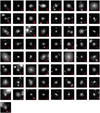 |
Fig. A.1 65 potential lens candidates considered as true positives in the common test data set in this work. The three grade A candidates are shown in Fig. 1 in the main text. 13 grade B and 52 grade C lens candidates are shown above with the respective grades shown in red in the bottom left corner of each subplot. Each image is 10′′ × 10′′. |
Appendix B Distribution of predicted scores from fine-tuning
We show the distribution of predictions, pLENS, on the 68 lens candidates given by the two fine-tuned EfficientNetB0 networks with pTHRESH = 0.5, namely Zoobot1 and Zoobot2, described in Sect. 3.1. Figure B.1 (left) shows the histogram of predicted scores for the 68 lens candidates using Zoobot1, with the grade A and B candidates shown to the right of this distribution in red and blue, respectively. These candidates are confidently classified as lenses. There is one grade B candidate that has a predicted score below the prediction threshold, thereby classified as a non-lens by Zoobot1. Figure B.1 (right) shows the predicted scores for the lens candidates using Zoobot2. Although Zoobot2 correctly classifies all grade A definite strong lens candidates, it is not as confident in its prediction of the grade B candidates. The predictions of the grade C candidates vary the most for both networks, shown in green. This is in agreement with the fact that grade C candidates are less likely to be lenses.
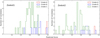 |
Fig. B.1 Distribution of predicted scores by Zoobot1 (left) and Zoobot2 (right) for lens candidates across all grades. Grade A lens candidates are confidently identified by both networks, shown to the right of the distribution in red at a high value of pLENS. Grade B predicted scores are shown in blue and are more varied for Zoobot2. The predicted scores for grade C lens candidates have the most variation amongst grades, shown in green, for both networks illustrating that Zoobot1 and Zoobot2 are not as confident in identifying grade C lens candidates. |
Appendix C False positives
Here, we show the common morphologies frequently occurring as false positives in the classification by all networks in this work. These morphologies include spiral galaxies, such as edge-on and face-on spirals, and spirals with prominent arms. Also common are stamps with multiple sources, and stamps with defective pixels that fall near the edges of the Perseus ERO footprint. Figure C.1 shows the false positives found by Zoobot1 with the predicted score, pLENS, shown in red in the top left corner of each subplot. Figure C.2 shows the false positives found by the 4-layer CNN described in Sect. 3.4, which are common to the false positives found by Zoobot1, with the respective predicted scores shown in the top left corner of each subplot. Finally, Fig. C.3 shows the false positives found by U-Denselens, described in Sect. 3.5, showing agreement in common morphologies that are misclassified as lenses to the other two networks shown here.
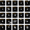 |
Fig. C.1 Example of 25 out of 547 false positives (NFP in Table 1) found by Zoobot1 in the common test set. Each panel contains the predicted score, pLENS, for each false positive, along with the true class (with False belonging to class ‘non-lens’). Each IE-band image is 10′′ × 10′′. |
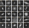 |
Fig. C.2 Example of 25 out of the 3068 false positives (NFP in Table 1) found by the 4-layer CNN with pTHRESH ≥ 0.7 in the common test set. Each panel contains the ID of the source and its corresponding predicted score, pLENS, for each false positive. There is a small fraction of stamps that fall near the borders of the Perseus footprint or with defective pixels. Each IE-band image is 10′′ × 10′′. |
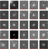 |
Fig. C.3 Example of 25 out of the 331 false positives (NFP in Table 1) found by the U-Denselens with the selection criteria in the common test set. Each panel contains the predicted score, pLENS, for each false positive along with the IC and ns. The ID of each source in shown in red in the bottom right. Frequently occurring morphologies are in agreement with other networks used in this work. Each IE-band image is 10′′ × 10′′. |
References
- Acevedo Barroso, J. A., O’Riordan, C. M., & Clément, B., e. a. 2025, A&A, 697, A14 [Google Scholar]
- Amara, A., de la Bella, L., Birrer, S., et al. 2021, J. Open Source Softw., 6, 3056 [Google Scholar]
- Andika, I. T., Jahnke, K., van der Wel, A., et al. 2023a, ApJ, 943, 150 [NASA ADS] [CrossRef] [Google Scholar]
- Andika, I. T., Suyu, S. H., Cañameras, R., et al. 2023b, A&A, 678, A103 [NASA ADS] [CrossRef] [EDP Sciences] [Google Scholar]
- Astropy Collaboration (Robitaille, T. P., et al.) 2013, A&A, 558, A33 [NASA ADS] [CrossRef] [EDP Sciences] [Google Scholar]
- Astropy Collaboration (Price-Whelan, A. M., et al.) 2018, AJ, 156, 123 [Google Scholar]
- Astropy Collaboration (Price-Whelan, A. M., et al.) 2022, ApJ, 935, 167 [NASA ADS] [CrossRef] [Google Scholar]
- Auger, M., Treu, T., Bolton, A., et al. 2009, ApJ, 705, 1099 [Google Scholar]
- Birrer, S., & Amara, A. 2018, Phys. Dark Universe, 22, 189 [NASA ADS] [CrossRef] [Google Scholar]
- Bolton, A. S., Burles, S., Koopmans, L. V. E., et al. 2008, ApJ, 682, 964 [Google Scholar]
- Buscema, M. 1998, Substance Use Misuse, 33, 233 [CrossRef] [PubMed] [Google Scholar]
- Caminha, G. B., Suyu, S. H., Grillo, C., & Rosati, P. 2022, A&A, 657, A83 [NASA ADS] [CrossRef] [EDP Sciences] [Google Scholar]
- Cañameras, R., Schuldt, S., Suyu, S., et al. 2020, A&A, 644, A163 [NASA ADS] [CrossRef] [EDP Sciences] [Google Scholar]
- Chen, T., Kornblith, S., Norouzi, M., & Hinton, G. 2020a, in Proceedings of Machine Learning Research, 119, Proceedings of the 37th International Conference on Machine Learning, eds. III, H. D., & Singh, A. (PMLR), 1597 [Google Scholar]
- Chen, T., Kornblith, S., Swersky, K., Norouzi, M., & Hinton, G. E. 2020b, in Advances in Neural Information Processing Systems, 33, eds. Larochelle, H., Ranzato, M., Hadsell, R., Balcan, M., & Lin, H. (Curran Associates, Inc.), 22243 [Google Scholar]
- Christ, C., Nord, B., Gozman, K., & Ottenbreit, K. 2020, in American Astronomical Society Meeting Abstracts, 235, 303.03 [Google Scholar]
- Collett, T. E. 2015, ApJ, 811, 20 [NASA ADS] [CrossRef] [Google Scholar]
- Collett, T. E., & Auger, M. W. 2014, MNRAS, 443, 969 [NASA ADS] [CrossRef] [Google Scholar]
- Cropper, M., Pottinger, S., Niemi, S., et al. 2016, in Space Telescopes and Instrumentation 2016: Optical, Infrared, and Millimeter Wave, 9904, eds. MacEwen, H. A., Fazio, G. G., Lystrup, M., Batalha, N., Siegler, N., & Tong, E. C. (SPIE) [Google Scholar]
- Cuillandre, J.-C., Bertin, E., Bolzonella, M., et al. 2025a, A&A, 697, A6 [Google Scholar]
- Cuillandre, J. C., Bolzonella, M., Boselli, A., et al. 2025b, A&A, 697, A11 [Google Scholar]
- Davies, A., Serjeant, S., & Bromley, J. M. 2019, MNRAS, 487, 5263 [NASA ADS] [CrossRef] [Google Scholar]
- de Jong, J. T., Verdoes Kleijn, G. A., Kuijken, K. H., & Valentijn, E. A. 2013, Exp. Astron., 35, 25 [NASA ADS] [CrossRef] [Google Scholar]
- Denzel, P., Mukherjee, S., & Saha, P. 2021, MNRAS, 506, 1815 [Google Scholar]
- Domínguez Sánchez, H., Huertas-Company, M., Bernardi, M., Tuccillo, D., & Fischer, J. L. 2018, MNRAS, 476, 3661 [Google Scholar]
- Euclid Collaboration (Schirmer, M., et al.) 2022, A&A, 662, A92 [NASA ADS] [CrossRef] [EDP Sciences] [Google Scholar]
- Euclid Collaboration (Ilic´, S., et al.) 2022, A&A, 657, A91 [CrossRef] [EDP Sciences] [Google Scholar]
- Euclid Collaboration (Scaramella, R., et al.) 2022, A&A, 662, A112 [NASA ADS] [CrossRef] [EDP Sciences] [Google Scholar]
- Euclid Collaboration (Aussel, B., et al.) 2024, A&A, 689, A274 [NASA ADS] [CrossRef] [EDP Sciences] [Google Scholar]
- Euclid Collaboration (Leuzzi, L., et al.) 2024, A&A, 681, A68 [NASA ADS] [CrossRef] [EDP Sciences] [Google Scholar]
- Euclid Collaboration (Castander, F., et al.) 2025, A&A, 697, A5 [Google Scholar]
- Euclid Collaboration (Cropper, M., et al.) 2025, A&A, 697, A2 [Google Scholar]
- Euclid Collaboration (Jahnke, K., et al.) 2025, A&A, 697, A3 [Google Scholar]
- Euclid Collaboration (Mellier, Y., et al.) 2025, A&A, 697, A1 [Google Scholar]
- European Space Agency 2024, Euclid Early Release Observations, https://doi.org/10.57780/esa-qmocze3 [Google Scholar]
- Faber, S., & Jackson, R. E. 1976, ApJ, 204, 668 [NASA ADS] [CrossRef] [Google Scholar]
- Gentile, F., Tortora, C., Covone, G., et al. 2022, MNRAS, 510, 500 [Google Scholar]
- Harris, C. R., Millman, K. J., van der Walt, S. J., et al. 2020, Nature, 585, 357 [NASA ADS] [CrossRef] [Google Scholar]
- Hayat, M. A., Stein, G., Harrington, P., Lukic´, Z., & Mustafa, M. 2021, ApJ, 911, L33 [NASA ADS] [CrossRef] [Google Scholar]
- He, K., Zhang, X., Ren, S., & Sun, J. 2016, in Proceedings of the IEEE conference on computer vision and pattern recognition, 770 [Google Scholar]
- He, K., Gkioxari, G., Dollár, P., & Girshick, R. 2017, in 2017 IEEE International Conference on Computer Vision (ICCV), 2980 [Google Scholar]
- He, K., Fan, H., Wu, Y., Xie, S., & Girshick, R. 2020, in Proceedings of the IEEE/CVF Conference on Computer Vision and Pattern Recognition (CVPR) [Google Scholar]
- Hecht-Nielsen, R. 1992, in Neural Networks for Perception (Elsevier), 65 [CrossRef] [Google Scholar]
- Howard, A., Sandler, M., Chu, G., et al. 2019, in Proceedings of the IEEE/CVF International Conference on Computer Vision, 1314 [Google Scholar]
- Hu, J., Shen, L., & Sun, G. 2018, in Proceedings of the IEEE Conference on Computer Vision and Pattern Recognition, 7132 [Google Scholar]
- Huang, G., Liu, Z., Van Der Maaten, L., & Weinberger, K. Q. 2017, in Proceedings of the IEEE Conference on Computer Vision and Pattern Recognition (CVPR), 4700 [Google Scholar]
- Huertas-Company, M., Guo, Y., Ginzburg, O., et al. 2020, MNRAS, 499, 814 [NASA ADS] [CrossRef] [Google Scholar]
- Huertas-Company, M., Sarmiento, R., & Knapen, J. H. 2023, RAS Tech. Instrum., 2, 441 [NASA ADS] [CrossRef] [Google Scholar]
- Hunter, J. D. 2007, Comput. Sci. Eng., 9, 90 [NASA ADS] [CrossRef] [Google Scholar]
- Jacobs, C., Glazebrook, K., Qin, A., & Collett, T. 2022, Astron. Comput., 38, 100535 [NASA ADS] [CrossRef] [Google Scholar]
- Kingma, D. P., & Ba, J. 2015, in 3rd International Conference on Learning Representations, ICLR 2015, San Diego, CA, USA, May 7-9, 2015, Conference Track Proceedings, eds. Bengio, Y., & LeCun, Y. [Google Scholar]
- Koopmans, L. V. E., Bolton, A., Treu, T., et al. 2009, ApJ, 703, L51 [NASA ADS] [CrossRef] [Google Scholar]
- Lanusse, F., Ma, Q., Li, N., et al. 2018, MNRAS, 473, 3895 [Google Scholar]
- Laureijs, R., Amiaux, J., Arduini, S., et al. 2011, arXiv e-prints [arXiv:1110.3193] [Google Scholar]
- LeCun, Y., Boser, B., Denker, J. S., et al. 1989, Neural Computat., 1, 541 [CrossRef] [Google Scholar]
- Lehar, J., Falco, E. E., Kochanek, C. S., et al. 2000, ApJ, 536, 584 [NASA ADS] [CrossRef] [Google Scholar]
- Li, R., Shu, Y., & Wang, J. 2018, MNRAS, 480, 431 [NASA ADS] [CrossRef] [Google Scholar]
- Li, R., Napolitano, N. R., Tortora, C., et al. 2020, ApJ, 899, 30 [Google Scholar]
- Li, R., Napolitano, N. R., Spiniello, C., et al. 2021, ApJ, 923, 16 [NASA ADS] [CrossRef] [Google Scholar]
- Li, T., Collett, T. E., Krawczyk, C. M., & Enzi, W. 2024, MNRAS, 527, 5311 [Google Scholar]
- Limousin, M., Kneib, J.-P., & Natarajan, P. 2005, MNRAS, 356, 309 [Google Scholar]
- Manjón-García, A. 2021, PhD thesis, University of Cantabria (Spain) [Google Scholar]
- Masters, K. L. 2019, Proc. Int. Astron. Union, 14, 205 [CrossRef] [Google Scholar]
- Meneghetti, Bartelmann, M., Dolag, K., et al. 2005, A&A, 442, 413 [NASA ADS] [CrossRef] [EDP Sciences] [Google Scholar]
- Metcalf, Meneghetti, M., Avestruz, C., et al. 2019, A&A, 625, A119 [NASA ADS] [CrossRef] [EDP Sciences] [Google Scholar]
- Miralda-Escude, J. 1991, ApJ, 370, 1 [Google Scholar]
- Möller, O., Natarajan, P., Kneib, J.-P., & Blain, A. 2002, ApJ, 573, 562 [Google Scholar]
- More, A., Cañameras, R., Jaelani, A. T., et al. 2024, MNRAS, 533, 525 [CrossRef] [Google Scholar]
- Nagam, B., Koopmans, L. V. E., Valentijn, E. A., et al. 2023, MNRAS, 523, 4188 [NASA ADS] [CrossRef] [Google Scholar]
- Nagam, B., Koopmans, L. V. E., Valentijn, E. A., et al. 2024, MNRAS, 533, 1426 [Google Scholar]
- Newton, E. R., Marshall, P. J., Treu, T., et al. 2011, ApJ, 734, 104 [NASA ADS] [CrossRef] [Google Scholar]
- Nord, B., Buckley-Geer, E., Lin, H., et al. 2016, ApJ, 827, 51 [NASA ADS] [CrossRef] [Google Scholar]
- O’Riordan, C. M., Oldham, L. J., Nersesian, A., et al. 2025, A&A, 694, A145 [NASA ADS] [CrossRef] [EDP Sciences] [Google Scholar]
- Petrillo, C. E., Tortora, C., Chatterjee, S., et al. 2017, MNRAS, 472, 1129 [Google Scholar]
- Petrillo, C. E., Tortora, C., Chatterjee, S., et al. 2019a, MNRAS, 482, 807 [NASA ADS] [Google Scholar]
- Petrillo, C. E., Tortora, C., Vernardos, G., et al. 2019b, MNRAS, 484, 3879 [Google Scholar]
- Pourrahmani, M., Nayyeri, H., & Cooray, A. 2018, ApJ, 856, 68 [NASA ADS] [CrossRef] [Google Scholar]
- Powell, D. M., Vegetti, S., McKean, J. P., et al. 2023, MNRAS, 524, L84 [NASA ADS] [CrossRef] [Google Scholar]
- Radosavovic, I., Johnson, J., Xie, S., Lo, W.-Y., & Dollar, P. 2020, in Proceedings of the IEEE/CVF Conference on Computer Vision and Pattern Recognition, 10428 [Google Scholar]
- Rezaei, S., McKean, J. P., Biehl, M., de Roo, W., & Lafontaine, A. 2022, MNRAS, 517, 1156 [NASA ADS] [CrossRef] [Google Scholar]
- Ronneberger, O., Fischer, P., & Brox, T. 2015, in International Conference on Medical image computing and computer-assisted intervention (Springer), 234 [Google Scholar]
- Schaefer, C., Geiger, M., Kuntzer, T., & Kneib, J.-P. 2018, A&A, 611, A2 [NASA ADS] [CrossRef] [EDP Sciences] [Google Scholar]
- Scoville, N., Aussel, H., Brusa, M., et al. 2007, ApJS, 172, 1 [Google Scholar]
- Shu, Y., Brownstein, J. R., Bolton, A. S., et al. 2017, ApJ, 851, 48 [Google Scholar]
- Simonyan, K., & Zisserman, A. 2015, in 3rd International Conference on Learning Representations, ICLR 2015, San Diego, CA, USA, May 7-9, 2015, Conference Track Proceedings [Google Scholar]
- Spiniello, C., Barnabè, M., Koopmans, L. V. E., & Trager, S. C. 2015, MNRAS, 452, L21 [Google Scholar]
- Stein, G., Blaum, J., Harrington, P., Medan, T., & Lukic´, Z. 2022, ApJ, 932, 107 [NASA ADS] [CrossRef] [Google Scholar]
- Storfer, C., Huang, X., Gu, A., et al. 2022, ApJ, submitted [arXiv:2206:02764] [Google Scholar]
- Suyu, S. H., Marshall, P. J., Auger, M. W., et al. 2010, ApJ, 711, 201 [Google Scholar]
- Szegedy, C., Liu, Wei, Jia, Yangqing, et al. 2015, in Proceedings of the IEEE conference on computer vision and pattern recognition, 1 [Google Scholar]
- Szegedy, C., Vanhoucke, V., Ioffe, S., Shlens, J., & Wojna, Z. 2016, in Proceedings of the IEEE Conference on Computer Vision and Pattern Recognition, 2818 [Google Scholar]
- Tan, M., & Le, Q. 2019, in Proceedings of the 36th International Conference on Machine Learning, 97, eds. Chaudhuri, K., & Salakhutdinov, R. (PMLR), 6105 [Google Scholar]
- Tan, M., & Le, Q. 2021, in Proceedings of Machine Learning Research, 139, Proceedings of the 38th International Conference on Machine Learning, eds. Meila, M., & Zhang, T. (PMLR), 10096 [Google Scholar]
- Teimoorinia, H., Bluck, A. F., & Ellison, S. L. 2016, MNRAS, 457, 2086 [NASA ADS] [CrossRef] [Google Scholar]
- Thuruthipilly, H., Zadrozny, A., Pollo, A., & Biesiada, M. 2022, A&A, 664, A4 [NASA ADS] [CrossRef] [EDP Sciences] [Google Scholar]
- Treu, T., & Koopmans, L. V. E. 2002, ApJ, 575, 87 [NASA ADS] [CrossRef] [Google Scholar]
- van den Oord, A., Li, Y., & Vinyals, O. 2018, arXiv e-prints [arXiv:1807.03748] [Google Scholar]
- Vegetti, S., Birrer, S., Despali, G., et al. 2024, Space Sci. Rev., 220, 58 [CrossRef] [Google Scholar]
- Walmsley, M., Scaife, A. M. M., Lintott, C., et al. 2022, MNRAS, 513, 1581 [NASA ADS] [CrossRef] [Google Scholar]
- Walmsley, M., Allen, C., Aussel, B., et al. 2023, J. Open Source Softw., 8, 5312 [NASA ADS] [CrossRef] [Google Scholar]
- Wilde, J., Serjeant, S., Bromley, J. M., et al. 2022, MNRAS, 512, 3464 [Google Scholar]
- Wilde, J. W. 2023, PhD thesis, The Open University, https://oro.open.ac.uk/94777/ [Google Scholar]
- Willett, K. W., Lintott, C. J., Bamford, S. P., et al. 2013, MNRAS, 435, 2835 [Google Scholar]
- Xie, S., Girshick, R. B., Dollár, P., Tu, Z., & He, K. 2016, in Proceedings of the IEEE Conference on Computer Vision and Pattern Recognition, 5987 [Google Scholar]
- You, K., Kou, Z., Long, M., & Wang, J. 2020, in Neural Information Processing Systems [Google Scholar]
- Zitrin, A., Rosati, P., Nonino, M., et al. 2012, ApJ, 749, 97 [NASA ADS] [CrossRef] [Google Scholar]
All Tables
Performance metrics for the various models with their pTHRESH values, based on the common test set of 12 086 stamps.
All Figures
|
Fig. 1 Three grade A candidate lenses found by a visual inspection of 12 086 stamps from the Perseus cluster showing clear lensing features. Each IE-band image is 10′′ × 10′′. Detailed lens models for these candidates are shown in Appendix C of Acevedo Barroso et al. (2025). |
| In the text | |
|
Fig. 2 Layers that construct the U-Net Naberrie including an encoder, a decoder, and a classifier. The arrows represent skip connections, connecting extracted features from the encoder section to the decoder section. |
| In the text | |
|
Fig. 3 Scheme of the architecture of the 4-layer CNN. The 4-layer CNN takes an 100 × 100 pixel IE-band image as input, and extracts features through blocks of convolution layers and max-pooling layers, with ReLU activation functions. The final fully-connected layer uses a sigmoid activation to produce a probability score as output, with 1 belonging to class lens. |
| In the text | |
|
Fig. 4 ROC curves for the networks described in Section 3. Performance of the Zoobot networks are shown in panel (a), Naberrie and MRC networks are shown in (b), NG, 4-layer CNN, and ResNet-18 are shown in (c), and Denselens and LencCLR are shown in (d). The performance of the networks described in Sect. 3.7 are shown in (e), and (f) shows the CBEN networks at two voting values β = 0.3 and β = 0.0001, respectively. The orange diagonal line marked represents the expected performance of an entirely random classifier. The values in the legend of each subplot represent the true positive recovery for each network. Higher performance is represented in general by curves approaching the top-left corner of the plots. |
| In the text | |
|
Fig. 5 Examples of correctly identified candidate lenses (or true positives) by Zoobot1 in the IE-band. The grade of each candidate is shown at the bottom of each subplot. Each subplot contains the predicted score, pLENS for that candidate along with the true class (with True belonging to class ‘lens’). Each candidate lens image is 10′′ × 10′′. |
| In the text | |
|
Fig. 6 Contamination rate, or NFP/NTP ratio, of the potential candidate lens sample of each network assuming a fixed FPR of 5%. Networks with a contamination rate >100 are not included in this comparison. The value given above each network shows the number of false positives found for every true candidate lens in the Perseus cluster data. |
| In the text | |
|
Fig. A.1 65 potential lens candidates considered as true positives in the common test data set in this work. The three grade A candidates are shown in Fig. 1 in the main text. 13 grade B and 52 grade C lens candidates are shown above with the respective grades shown in red in the bottom left corner of each subplot. Each image is 10′′ × 10′′. |
| In the text | |
|
Fig. B.1 Distribution of predicted scores by Zoobot1 (left) and Zoobot2 (right) for lens candidates across all grades. Grade A lens candidates are confidently identified by both networks, shown to the right of the distribution in red at a high value of pLENS. Grade B predicted scores are shown in blue and are more varied for Zoobot2. The predicted scores for grade C lens candidates have the most variation amongst grades, shown in green, for both networks illustrating that Zoobot1 and Zoobot2 are not as confident in identifying grade C lens candidates. |
| In the text | |
|
Fig. C.1 Example of 25 out of 547 false positives (NFP in Table 1) found by Zoobot1 in the common test set. Each panel contains the predicted score, pLENS, for each false positive, along with the true class (with False belonging to class ‘non-lens’). Each IE-band image is 10′′ × 10′′. |
| In the text | |
|
Fig. C.2 Example of 25 out of the 3068 false positives (NFP in Table 1) found by the 4-layer CNN with pTHRESH ≥ 0.7 in the common test set. Each panel contains the ID of the source and its corresponding predicted score, pLENS, for each false positive. There is a small fraction of stamps that fall near the borders of the Perseus footprint or with defective pixels. Each IE-band image is 10′′ × 10′′. |
| In the text | |
|
Fig. C.3 Example of 25 out of the 331 false positives (NFP in Table 1) found by the U-Denselens with the selection criteria in the common test set. Each panel contains the predicted score, pLENS, for each false positive along with the IC and ns. The ID of each source in shown in red in the bottom right. Frequently occurring morphologies are in agreement with other networks used in this work. Each IE-band image is 10′′ × 10′′. |
| In the text | |
Current usage metrics show cumulative count of Article Views (full-text article views including HTML views, PDF and ePub downloads, according to the available data) and Abstracts Views on Vision4Press platform.
Data correspond to usage on the plateform after 2015. The current usage metrics is available 48-96 hours after online publication and is updated daily on week days.
Initial download of the metrics may take a while.