| Issue |
A&A
Volume 692, December 2024
|
|
|---|---|---|
| Article Number | A72 | |
| Number of page(s) | 22 | |
| Section | Numerical methods and codes | |
| DOI | https://doi.org/10.1051/0004-6361/202347072 | |
| Published online | 03 December 2024 | |
HOLISMOKES
XI. Evaluation of supervised neural networks for strong-lens searches in ground-based imaging surveys
1
Max-Planck-Institut für Astrophysik,
Karl-Schwarzschild-Str. 1,
85748
Garching, Germany
2
Technical University of Munich, TUM School of Natural Sciences, Department of Physics,
James-Franck-Straße 1,
85748
Garching, Germany
3
Aix Marseille Univ, CNRS, CNES, LAM,
Marseille,
France
4
Dipartimento di Fisica, Università degli Studi di Milano,
via Celoria 16,
20133
Milano, Italy
5
INAF - IASF Milano,
via A. Corti 12,
20133
Milano, Italy
6
Purple Mountain Observatory,
No. 10 Yuanhua Road, Nanjing,
Jiangsu,
210033, PR China
7
Institute of Astronomy and Astrophysics, Academia Sinica,
11F of ASMAB, No. 1, Section 4, Roosevelt Road,
Taipei
10617, Taiwan
8
Kindai University, Faculty of Science and Engineering,
Osaka
577-8502, Japan
9
Astronomy Research Group and Bosscha Observatory, FMIPA, Institut Teknologi Bandung,
Jl. Ganesha 10,
Bandung
40132, Indonesia
10
U-CoE AI-VLB, Institut Teknologi Bandung,
Jl. Ganesha 10,
Bandung
40132, Indonesia
11
Technical University of Munich, Department of Informatics,
Boltzmann-Str. 3,
85748
Garching, Germany
12
Kavli Institute for the Physics and Mathematics of the Universe (WPI), UTIAS, The University of Tokyo,
Kashiwa, Chiba
277-8583, Japan
13
The Inter-University Centre for Astronomy and Astrophysics (IUCAA),
Post Bag 4,
Ganeshkhind,
Pune
411007, India
★ Corresponding author; This email address is being protected from spambots. You need JavaScript enabled to view it.
Received:
2
June
2023
Accepted:
21
October
2024
Abstract
While supervised neural networks have become state of the art for identifying the rare strong gravitational lenses from large imaging data sets, their selection remains significantly affected by the large number and diversity of non-lens contaminants. This work evaluates and compares systematically the performance of neural networks in order to move towards a rapid selection of galaxy-scale strong lenses with minimal human input in the era of deep, wide-scale surveys. We used multiband images from PDR2 of the Hyper-Suprime Cam (HSC) Wide survey to build test sets mimicking an actual classification experiment, with 189 securely-identified strong lenses from the literature over the HSC footprint and 70 910 non-lens galaxies in COSMOS covering representative lens-like morphologies. Multiple networks were trained on different sets of realistic strong-lens simulations and non-lens galaxies, with various architectures and data preprocessing, mainly using the deepest gri-bands. Most networks reached excellent area under the Receiver Operating Characteristic (ROC) curves on the test set of 71 099 objects, and we determined the ingredients to optimize the true positive rate for a total number of false positives equal to zero or 10 (TPR0 and TPR10). The overall performances strongly depend on the construction of the ground-truth training data and they typically, but not systematically, improve using our baseline residual network architecture presented in Paper VI (Cañameras et al., A&A, 653, L6). TPR0 tends to be higher for ResNets (≃ 10–40%) compared to AlexNet-like networks or G-CNNs. Improvements are found when (1) applying random shifts to the image centroids, (2) using square-root scaled images to enhance faint arcs, (3) adding z-band to the otherwise used gri-bands, or (4) using random viewpoints of the original images. In contrast, we find no improvement when adding g – αi difference images (where α is a tuned constant) to subtract emission from the central galaxy. The most significant gain is obtained with committees of networks trained on different data sets, with a moderate overlap between populations of false positives. Nearly-perfect invariance to image quality can be achieved by using realistic PSF models in our lens simulation pipeline, and by training networks either with large number of bands, or jointly with the PSF and science frames. Overall, we show the possibility to reach a TPR0 as high as 60% for the test sets under consideration, which opens promising perspectives for pure selection of strong lenses without human input using the Rubin Observatory and other forthcoming ground-based surveys.
Key words: gravitation / gravitational lensing: strong / methods: data analysis / cosmology: observations
© The Authors 2024
 Open Access article, published by EDP Sciences, under the terms of the Creative Commons Attribution License (https://creativecommons.org/licenses/by/4.0), which permits unrestricted use, distribution, and reproduction in any medium, provided the original work is properly cited.
This article is published in open access under the Subscribe to Open model.
Open Access funding provided by Max Planck Society.
1 Introduction
Galaxy-scale strong gravitational lenses have a number of important roles in characterizing the astrophysical processes underlying galaxy mass assembly and in constraining the cosmological framework in which these galaxies evolve (e.g., Shajib et al. 2022, and references therein). Strong lenses with time-variable background sources enable one-step measurements of cosmo-logical distances from the time delays between multiple lensed images, thus allowing constraints on the cosmic expansion rate to be obtained (e.g., Refsdal 1964; Wong et al. 2020; Shajib et al. 2023). Conducting studies with strongly lensed supernovae is one of the scientific goals of our Highly Optimized Lensing Investigations of Supernovae, Microlensing Objects, and Kinematics of Ellipticals and Spirals (HOLISMOKES, Suyu et al. 2020) program (see also Suyu et al. 2024, for a review). However, lensed supernovae are not common given the rarity of both strong lensing of galaxies and the occurrence of supernovae. There are several approaches to finding lensed supernovae. One way is to look for supernovae that are brighter than expected due to lensing magnification (e.g., Goldstein & Nugent 2017; Goldstein et al. 2019). Another way is to have a large sample of strong lenses, and to monitor these systems through either dedicated monitoring or cadenced image surveys in order to reveal supernovae occurring in the lensed galaxies (e.g., Shu et al. 2018; Craig et al. 2024). It is therefore desirable to augment existing samples of strong lenses. This effort will also be beneficial for studies of dark-matter and their deflectors (Shajib et al. 2022).
Deep, wide-scale surveys have the potential to yield large samples (~105) of strong lenses. Either alone or together, imaging and spectroscopic data sets can be relevant for this task, depending on the nature of the deflector and background source populations. For the galaxy-galaxy strong-lens category, the identification of spatially resolved multiple-lensed images forming around a central galaxy is an efficient selection technique that has been applied to several imaging surveys (e.g., Gavazzi et al. 2014; Marshall et al. 2016; Diehl et al. 2017). When the background source is compact and point-like, the lens system displays a multiple point-like lensed image. When the background source is spatially extended, the lens system displays arc-like lensed images that may even connect to form a ring. In the next years, the Euclid (Laureijs et al. 2011) and Roman telescopes (Green et al. 2012) and the Chinese Space Station Telescope (Gong et al. 2019) will significantly expand these imaging data sets in the optical and near-infrared from space. The Rubin Observatory Legacy Survey of Space and Time (LSST; Ivezić et al. 2019) will cover similar wavelengths from the ground, and in the radio, the Square Kilometer Array will complement the selection toward populations of dust-obscured higher-redshift sources mostly undetected in the optical and near-infrared (McKean et al. 2015). Since the strong-lens discovery rate scales with both depth and spatial coverage, these next-generation surveys are expected to transform the field and to increase the current sample of strong-lens candidates by at least two orders of magnitude (Collett 2015). This expected increase nonetheless relies on highly efficient, automated selection methods.
Machine learning techniques appeared in astronomy in the past decade, and supervised convolutional neural networks (CNNs; LeCun et al. 1998) have since played increasing roles in image analysis problems. Besides being used for morphological classification of galaxies (Dieleman et al. 2015; Walmsley et al. 2022), CNNs have also proven useful for estimating galaxy properties ranging from photometric redshifts (e.g. D’Isanto & Polsterer 2018; Schuldt et al. 2021a) to structural parameters (e.g., Tuccillo et al. 2018; Tohill et al. 2021; Li et al. 2022). Given the possibility to simulate large samples of strong lenses with highly realistic morphologies for training, supervised CNNs have become the state of the art for lens searches (Metcalf et al. 2019), and they have been used for lens modeling (e.g., Hezaveh et al. 2017; Schuldt et al. 2021b, 2023a; Pearson et al. 2021). Other semi-supervised and unsupervised lens-finding approaches are being developed (e.g., Cheng et al. 2020; Stein et al. 2022), but they do not yet offer a significant gain in classification accuracy.
Large samples of strong-lens candidates have been identified by applying supervised CNNs to existing surveys and by cleaning the network outputs visually (e.g., Petrillo et al. 2017; Jacobs et al. 2019a; Huang et al. 2021). Recently, Tran et al. (2022) conducted the first systematic spectroscopic confirmation of candidates selected through this process, finding a large majority of genuine strong lenses and a success rate of nearly 90%. Human inspection is nonetheless key to reaching this optimal purity. CNNs reach >99% accuracy for balanced data sets of lenses and non-lenses (e.g., Lanusse et al. 2018), but since the fraction of strong lenses only represents up to 10−3 of all galaxies per sky area, applying these networks to real survey data results in samples dominated by false positives. Nearly 97% of the candidates identified with the PanSTARRS CNN from Cañameras et al. (2020) were, for instance, discarded from the final list of high-quality candidates by visual inspection, a rate comparable to other lens finders in the literature.
Low ratios of high-quality candidates over network recommendations imply long visual inspection processes. Moreover, Rojas et al. (2023) show that grades attributed by groups of classifiers vary substantially, in particular for lenses with faint arcs and low Einstein radii, and continue to do so even when restricting to “expert classifiers”. Asking a single person to classify a sample of candidates multiple times also leads to substantial scatter in the output grades, especially for non-obvious lenses (see Shu et al. 2022; Rojas et al. 2023). Most classification biases can be minimized by requesting multiple (≳5–10) independent visual grades per candidate, but this further increases the need for human resources. The larger number of galaxies in the next-generation surveys will strongly complicate this process, even with crowdsourcing. The PanSTARRS lens finder from Cañameras et al. (2020), the DES lens finder from Jacobs et al. (2017, 2019b) and other contemporary CNN searches have typical false-positive rates of ~1–2%. For instance, when scaling the performance of the PanSTARRS lens finder to deeper, higher-quality imaging, we expect about 0.5 to 1 million CNN lens candidates to visually grade over the Rubin LSST footprint. This clearly shows the need to further test CNN selections and improve their recall (also known as the true-positive rate) with low contamination. Our subsequent strong-lens selection in Hyper-Suprime Cam imaging (Cañameras et al. 2021) already showed an improvement in this regard (see also Nagam et al. 2023).
In this work, we evaluate and compare the performance of supervised neural networks in order to reduce the need for human inspections for future surveys. In general, test sets drawn from strong-lens simulations and user-dependent selections of non-lens galaxies can only roughly mimic a classification experiment, given the variety of contaminants or image artifacts encountered in real survey data. In this study, we built representative test sets directly from survey data to robustly evaluate the actual network performance and contamination rates. We used multiband images from the Hyper-Suprime Cam Subaru Strategic Program (HSC-SSP; Aihara et al. 2018a) to train, validate, and test our networks while taking advantage of previous searches for galaxy-scale strong lenses conducted in this survey with non-machine learning techniques (Sonnenfeld et al. 2018, 2020; Wong et al. 2018; Chan et al. 2020; Jaelani et al. 2020). HSC-SSP also serves as testbed for the preparation of LSST with comparable imaging quality and a depth about 1 mag lower than the ten-year LSST stacks (for the LSST baseline design, Ivezić et al. 2019). A companion study (More et al. 2024) compares machine learning assisted strong-lens finders trained by independent teams using simulation pipelines that are not explored in this work (e.g., SIMCT, More et al. 2016). With various test sets based on real and simulated data, More et al. (2024) have gained insights on the network selection functions, and they complement this work that primarily focuses on optimizing the purity of strong-lens candidate samples.
The present paper is organized as follows. In Section 2, we introduce the overall procedure. The construction of data sets for training and testing the CNNs are described in Section 3, and the various network architectures are introduced in Section 4. Section 5 presents the tests of several neural networks and highlights the ingredients for reaching a higher performance. Section 6 further discusses the stability of the network predictions and Section 7 summarizes the results. We adopt the flat concordant ΛCDM cosmology with ΩM = 0.308 and ΩΛ = 1 – ΩM (Planck Collaboration XIII 2016) and with H0 = 72 km s−1 Mpc−1 (Bonvin et al. 2017).
2 Methodology
A comparison of algorithms for galaxy-scale lens searches was initiated by the Euclid consortium, using simulations from the Bologna lens factory project (Metcalf et al. 2019) based on the Millennium simulation (Lemson & Virgo Consortium 2006). This challenge demonstrated the higher performance of CNNs compared to traditional algorithms, not only for the classification of single-band, Euclid-like images, but also for multi-band data similar to ground-based surveys. Images for training and testing the networks were fully simulated, with the surface brightness of lens and non-lens galaxies inferred from the properties of their host dark-matter halo and semi-analytic galaxy formation models. Even though disk, bulge components, and spiral arms were also mocked up, the design of this challenge does not quantify the actual performance of lens-finding algorithms on real data. More realistics test sets drawn from observed images and including the main populations of lens-like contaminants (spirals, ring galaxies, groups) are needed to evaluate the ability of supervised neural networks in distinguishing strong lenses from the broad variety of non-lens galaxies and image artifacts present in survey data. In this paper, we aim at filling in this gap by comparing the performance of several deep learning strong-lens classifiers on real, multiband ground-based imaging observations including realistic number and diversity of lens-like galaxies that are non-lenses.
We used data from the second public data release (PDR2, Aihara et al. 2019) of the HSC-SSP. This deep, multiband survey is conducted with the wide-field HSC camera mounted on the 8.2m Subaru telescope and consists of three layers (Wide, Deep, and UltraDeep). We focused on the Wide layer which aims at imaging 1400 deg2 in the five broadband filters grizy with 5σ point-source sensitivities of 26.8, 26.4, 26.2, 25.4, and 24.7 mag, respectively. The PDR2 observations taken until January 2018 cover nearly 800 deg2 in all bands down to limiting magnitudes of 26.6, 26.2, 26.2, 25.3, and 24.5 mag in grizy, respectively, close to the survey specifications, with 300 deg2 having full-color full-depth observations. The seeing distributions have median and quartile values in arcsec of  ,
,  ,
,  ,
,  , and
, and  in g-, r-, i-, z-, and y-bands, respectively.
The tests in this paper were conducted on galaxies from HSC Wide PDR2 with at least one exposure in all five filters, including regions that do not reach full depth in all filters. Experiments were mainly conducted with the gri-bands that have optimal depth, with z-band added in some cases, and galaxies flagged with issues1 in HSC tables were discarded. We focused on the subset of extended galaxies with Kron radius larger than 0.8″ in the i-band and with i-band magnitudes lower (brighter) than 25 mag used by Schuldt et al. (2021a), in order to limit the data volume while only excluding the faintest, most compact galaxies that are unlikely to act as strong lenses. This provides a catalog of 62.5 million galaxies spanning a broad variety of morphological types. We note that this parent sample with i-band Kron radius ≥0.8″ and i < 25 mag is evenly distributed over the footprint, to account for the spatial variations in seeing and depth over the PDR2 images (see Aihara et al. 2019).
Rather than targeting all types of strong-lens configurations, which would be challenging for an individual algorithm, we focus here on the galaxy-galaxy systems which have a broad range of applications in astrophysics and cosmology. We intentionally avoid training and testing the networks on systems with complex lens potentials such as those with multiple galaxies, and systems with a main, isolated deflector and strong external shear from the lens environment. Lastly, the selection is aimed at optimizing the recall of systems with foreground luminous red galaxies (LRGs) which have the highest lensing cross-section (Turner et al. 1984), and with any type of background source. In particular, we focused on LRGs from the Sloan Digital Sky Survey (SDSS) with corresponding spectroscopic redshift and velocity dispersion measurements (Abolfathi et al. 2018) in order to simulate realistic lensed sources (which is described in more detail in Sect. 3.1.1). We intend to find the main ingredients to optimize the network contamination rates directly from the HSC images, without using strict pre-selections in color-color space, while also minimizing the need for human validation of the network outputs.
The neural networks were trained, validated and tested on image cutouts from PDR2 with constant sizes of 60 × 60 pixels (10″ × 10″), sufficient to cover the strong lensing features for galaxy-scale lenses with Einstein radii θE < 3″. Slightly different cutout sizes ranging from 50 × 50 pixels to 70 × 70 pixels were tested, but did not significantly impact the results. The GAMA09H field – which includes COSMOS – was systematically discarded for training and validation. This field was reserved for a detailed comparison of deep learning classifiers from several teams (More et al. 2024), and also used to test the dependence of the network inference on variations in seeing FWHM (see Section 6).
3 Data sets
3.1 Ground-truth data for training and validation
We followed a supervised machine learning classification procedure, by training the neural networks on various sets of strong-lens simulations and non-lens galaxies. The construction of these sets of positive and negative examples are described below. The resulting ground-truth data sets are balanced, with 50% positive and 50% negative examples.
3.1.1 Strong-lens simulations
The simulations of galaxy-scale strong gravitational lenses were obtained with the pipeline described in detail by Schuldt et al. (2021b, 2023a). Briefly, to produce highly realistic mocks capturing the properties of HSC images in the Wide layer, the pipeline paints lensed arcs on multiband HSC images of galaxies acting as strong-lens deflectors, using Singular Isothermal Ellipsoids (SIE) to model the foreground mass potentials. This approach enables the inclusion of light for neighboring galaxies and accounts for the small-scale variations in seeing and depth over the footprint. To assign a realistic SIE mass to each deflector, we focused on lens galaxies with robust spectroscopic redshifts, zspec, and velocity dispersions, vdisp, as described below. The SIE centroids, axis ratios, and position angles were then inferred from the i-band light profiles, with random perturbations following the mass-to-light offsets measured in SLACS lenses (Bolton et al. 2008). External shear was included in our simulations similarly as Schuldt et al. (2023a), using a flat distribution in shear strength between 0 and 0.1 to cover plausible values in real lens systems, and using random shear position angles. The sample of lens LRGs with zspec and vdisp measurements was selected from the SDSS catalogs. After excluding the flagged QSOs, we collected all LRGs from the BOSS (Abolfathi et al. 2018) and eBOSS (Bautista et al. 2018) catalogs with δvdisp < 100 km s−1 to cover the broadest redshift range possible. The resulting sample contains 50 220 LRGs within the HSC Wide footprint with a redshift distribution peaking at z ≃ 0.5 and extending out to z ≲ 1, and a velocity dispersion distribution peaking at vdisp ≃ 200 km s−1. In consequence, these LRGs cover the bright-end of the lens-galaxy luminosity function.
To include realistic source morphologies in our simulations we used high-resolution, high signal-to-noise ratio (S/N) images of distant galaxies from the Hubble Ultra Deep Field (HUDF; Beckwith et al. 2006) rather than simple parametric descriptions of the source light profiles. Using real sources accounts for the diversity and complexity of high-redshift galaxies. We focused on the 1574 HUDF sources with spectroscopic redshift measurements from MUSE (Inami et al. 2017), resulting in a red-shift distribution covering up to z ≃ 6, with two main peaks at z ≃ 0.5–1 and z ≃ 3–3.5. This distribution closely matches the redshift range of lensed galaxies in the test set with measured zspec. The color distribution of sources in both sets also broadly match. Before importing the HST exposures into the simulation pipeline, the neighboring galaxies around the HUDF sources with measured zspec were masked with SExtractor (Bertin & Arnouts 1996) as described in Schuldt et al. (2021b). Color corrections were also applied to match HST filter passbands to the HSC zeropoints.
The deflectors from the LRG sample were paired with random HUDF sources to satisfy specific criteria on the parameter distributions. The Einstein radius, source color, and lens redshift distributions were controled during this stage to produce different data sets (see Section 5.2). A given lens LRG was included up to four times with distinct rotations of the HSC cutouts by k × π/2, where k = 0,1,2,3; for each possible rotation of a lens LRG, a different background source and source position was paired with the LRG. For a given lens-source pair, the source was randomly placed in the source plane, over regions satisfying a lower limit on the magnification factor μ of the central pixel, and then lensed with the GLEE software (Suyu & Halkola 2010; Suyu et al. 2012). The lensed source was convolved with the subsampled PSF model for the location of the lens released in PDR22, and scaled to the HSC pixel size and to the HSC photometric zeropoints. Lensed images were finally coadded with the lens HSC cutout. To ensure that all simulations include bright, well-detected and multiple lensed images/arcs, we required that the brightest pixel over the multiple lensed images/arcs exceeds the background noise level over the lens LRG cutout by a factor (S/N)bkg,min, either in g- or i-band depending on the source color. While most lensed images are necessarily blended with the lens galaxies, we further required that the brightest pixel over the lensed images/arcs has a flux higher than the lens galaxy at that position by a factor Rsr/ls,min. For each lens-source pair, the source was randomly moved in the source plane until the lensed images satisfy these conditions; if the conditions were not satisfied after 20 iterations, then the source brightness was artificially boosted by 1 mag in each band. The procedure was repeated until reaching the maximal magnitude boost of 5 mag.
Our baseline data set includes 43 750 mock lenses with a nearly uniform Einstein radius distribution over the range 0.75″–2.5″, and with lensed images having μ ≥ 5, (S/N)bkg,min = 5, and Rsr/ls,min = 1.5 (see Fig. 1). This lower limit on θE approaches the median seeing FWHM in g- and r-bands, and helps obtain multiple images that meet our brightness and deblending criteria. The matching of lens-source pairs applied stronger weights on lens LRGs at zd > 0.7 in order to increase the relative fraction of fainter and redder lenses in the data set. Similarly, the number of red sources was boosted to increase the fraction of red lensed arcs by a factor of two compared to the original HUDF sample. None of these criteria significantly altered the final Einstein radius distribution. Other sets of simulations tested in Section 5.2 use alternative parameter distributions and different values of μ and (S/N)bkg,min, and they contain between 30 000 and 45 000 mocks.
3.1.2 Selection of non-lenses
The samples of non-lens galaxies used in our various ground-truth data sets were selected from the parent sample of galaxies with i-band Kron radius ≥0.8″ to match the restriction on the lens sample. In order to investigate the classification performance as a function of the morphological type of galaxies included in the training sets, we extracted specific samples of galaxies using publications in the literature. We focused on the galaxy types forming the majority of non-lens contaminants, in order to help the neural networks learn models that are able to identify the strong lensing features while excluding the broad variety of non-lens galaxies. In the following, we give specific details on each of these samples.
The extended arms of spiral galaxies can closely resemble the radial arcs formed by strongly lensed galaxies, especially for low inclination angles. Given that spiral arms predominantly contain young, blue stellar populations, akin to the colors of high-redshift lensed galaxies, the two types can present very similar morphologies in ground-based seeing-limited optical images. We based our selection of spirals on the catalog of Tadaki et al. (2020). This study visually identifies 1447 S-spirals and 1382 Z-spirals from HSC PDR2 images to train a CNN and find a larger sample of nearly 80 000 spirals with i < 20 mag over 320 deg2 in the Wide layer. Given the construction of their training set, the selection of Tadaki et al. (2020) is mainly sensitive to large, well-resolved spiral arms with clear winding direction. We tried various cuts on the galaxy sizes, finding that i-band Kron radii ≤2″ is an optimal cut to obtain a sufficient number of 40 000 spirals while ensuring that spiral arms fall at 1–3″ from the galaxy centroids and within our 10″ × 10″ cutouts.
The networks in our study were trained to identify the importance of strong lensing features such as point-like or arc-like lensed images around lens galaxies. To distinguish these features from isolated LRGs, we included large fractions of isolated LRGs in the data sets. To focus on the brightest, massive LRGs that are likely to act as strong lenses, we selected LRGs from the same parent sample as in our simulations. Moreover, groups of bright galaxies within 5–10″ in projection that mimic the distribution of multiple images are frequently misclassified as strong lenses. We constructed a sample of compact groups using the catalog of groups and clusters from Wen et al. (2012) based on SDSS-III. The richest structures were selected by setting the number of galaxies within a radius of r200 to N200 > 10, and by requiring at least three bright galaxies with rKron < 23 within 10″. The cutouts were then centered on the HSC galaxy closest to the position given by Wen et al. (2012). Finally, random non-lens galaxies were selected from the parent sample with i-band Kron radius ≥ 0.8″, after excluding all confirmed and candidates lenses from the literature, using our compilation up to December 2022 (Cañameras et al. 2021 and references therein). Various cuts on the r-band Kron magnitudes were tested, including the criteria r < 23 mag that covers the majority of LRG lens galaxies, but we obtained better performance for random non-lenses down to the limiting magnitude of HSC Wide.
Other classes such as edge-on galaxies, rings, and mergers can possibly confuse the neural networks (see Rojas et al. 2022) but were not directly included in the non-lens set. While citizen science projects based on SDSS (Willett et al. 2013), HST (Willett et al. 2017), and DECaLS (Walmsley et al. 2022) include such morphological types in their classification, they overlap only partially with the HSC footprint and do not provide the ≳103 examples required to further tune our data sets. Studies based on unsupervised machine learning algorithms (e.g., Hocking et al. 2018; Martin et al. 2020; Cheng et al. 2021) are allowing efficient separation of early- and late-type galaxies, but their ability to identify pure sample of rare galaxy types needs further confirmation. In the future, outlier detection could become an alternative (e.g., Margalef-Bentabol et al. 2020).
The non-lenses in our baseline ground-truth data set include 33% spirals, 27% LRGs, 6% groups, and 33% random galaxies. Other alternative data sets tested in Section 5.2 either use only one of these morphological types, or vary their relative proportion. Similar to the LRGs in the lens simulations, non-lens galaxies cover random position over the entire HSC PDR2 footprint. This ensures that galaxies in our training set sample representative seeing FWHM values and image depth, which is particularly important given that only about 40% of the area we consider reaches nominal depth in all five bands.
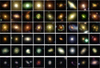 |
Fig. 1 Positive (lens) and negative (non-lens) examples in our baseline ground-truth data set. The first, second, and third rows show mock lenses with 0.75″ <θE < 1.30″, 1.30″ < θE < 1.90″, and 1.90″ < θE < 2.50″, respectively. The fourth, fifth, and sixth rows show examples of LRGs, spirals, and random galaxies from the parent sample of galaxies with i-band Kron radius ≥ 0.8″, respectively. This corresponds to the three main classes of negative examples. Cutouts have sizes of 10″ × 10″. |
3.2 Content of the test sets
The performance of our classification networks were evaluated on two specific test sets, which are also drawn from the input sample of real galaxies in HSC PDR2 with i-band Kron radius ≥0.8″. While the discussion resulting from this analysis is directly related to the construction of these test sets, we expect the results to be easily transferrable to other HSC data releases and to external surveys with comparable image depth and quality.
3.2.1 Strong lenses from the literature
Spectroscopically confirmed or high-quality candidate galaxy-scale strong lenses from the Survey of Gravitationally-lensed Objects in HSC Imaging (SuGOHI) were used to test the neural network recall (Sonnenfeld et al. 2018, 2020; Wong et al. 2018; Chan et al. 2020; Jaelani et al. 2020). These systems have been previously discovered with multiband imaging from the Wide layer using non-machine learning selection techniques followed by visual inspection from experts. As their selection relies on the combination of various techniques – such as searches for spectral lines in blended spectra, lens light subtraction and lens modeling, or crowdsourcing – these systems form a representative subset of the overall population of detectable strong lenses in HSC. We selected the highest-quality SuGOHI lenses classified as grade A or B according to the criteria listed in Sonnenfeld et al. (2018). Given our focus on galaxy-scale lenses, we visually excluded 27 systems with image separations ≫3″ typical of group-scale lenses, or with lensed arcs significantly perturbed by nearby galaxies or large-scale mass components. We checked that none of the remaining lenses contains background quasars, and we restricted to lens galaxies with i-band Kron radius above 0.8″ to match our overall search sample. This results in a sizeable set of 189 securely identified lenses from the literature. Of these, 44 are grade-A systems in the SUGOHI database, and 145 are reported as grade B. In total, 88 systems have spectroscopic redshifts for the lens galaxies, and 20 have zspec measured for both the lens and source. For the remainder of this paper, we refer to these 189 confirmed or securely identified lens candidate as our test lenses.
Some of these SuGOHI lenses and lens candidates were found in earlier data releases covering smaller areas than PDR2, but the images originally used for discovery also cover gri-bands, with depth comparable to PDR2 (see Aihara et al. 2018b, 2019). In terms of angular separation between the lens center and multiple lensed images, the various SuGOHI classification algorithms apply lens light subtraction prior to the arc identification and lens modeling steps, which presumably helps identify more compact systems (see Sonnenfeld et al. 2018). The subset with detailed lensing models nonetheless have Einstein radii in the range 0.80–1.80", which is representative of the distribution over the entire sample peaking at θE ≃ 1.2″–1.3″. This indicates that the 189 test lenses have both well-deblended lens and source components and sufficiently high S/N in gri images from the PDR2 Wide layer, and that all should be recovered via deep-learning classification of raw images. In contrast, additional lenses and lens candidates that are not detected and spatially resolved in PDR2 gri cutouts (e.g., from SDSS fiber spectra, Bolton et al. 2008; Brownstein et al. 2012; Shu et al. 2016) were discarded for testing.
3.2.2 Non-lenses in the COSMOS field
We collected a large sample of non-lens galaxies in the COSMOS field to quantify the ability of our networks to exclude the broad variety of contaminants, and to obtain the most realistic false-positive rate estimates for a real classification setup. By focusing on the well-studied COSMOS field, we can firmly exclude all strong lenses and conduct these estimates automatically. Non-lenses were selected from our parent sample with Kron radius larger than 0.8″ and without flagged cutouts. We note that these flags exclude galaxies with unreliable photometry, but do not exclude cutouts with partial coverage in one or several bands, with diffraction spikes, or other artifacts. Moreover, Aihara et al. (2019) show that a few artifacts remain in the coadded frames of the Wide layer, such as compact artifacts near static sources, and artifacts located in regions with only one or two exposures in PDR2. These were intentionally kept in our test set. All confirmed lenses and lens candidates were excluded using the MasterLens database3, Faure et al. (2008), Pourrahmani et al. (2018), Li et al. (2021), and SuGOHI papers, leaving 70910 unique non-lens galaxies.
To match our overall approach, we focused on the Wide layer and ignored COSMOS images from Deep and UDeep layers. In PDR2, the COSMOS field is observed to full-depth in all filters, which is not the case for all HSC fields included in our parent sample. We probed differences in image quality between COSMOS and the overall footprint by plotting distributions of the number of input frames per coadd and of the seeing FWHM in gri-bands, for the 70910 non-lenses in COSMOS and a random subset of our parent sample. The distributions of number of frames per band roughly match for both samples. Only the tail of ≲10% galaxies with ≤3 frames per stack disappears in the COSMOS field. The distributions of seeing FWHMs differ more strongly, since the small COSMOS field was observed with atmospheric conditions closest to the survey specifications. Fortunately, in COSMOS, the median seeing FWHMs in gri-bands closely match the values over the HSC footprint listed in Section 2, with only a smaller scatter. The quality of PDR2 images in our COSMOS test set are therefore roughly representative of the overall HSC Wide footprint.
4 The network architectures
In this section, we test state-of-the-art CNN and ResNet architectures, starting with baseline architectures and exploring variations around this baseline. We describe these architectures together with alternative group-equivariant neural networks aimed at improving the stability with respect to image rotations. More advanced supervised machine learning approaches are increasingly used in astronomy. For instance, Thuruthipilly et al. (2022) implemented self-attention-based architectures (Transformers, Vaswani et al. 2017) for lens searches using simulated data from the Bologna lens challenge. Such modern neural network models remain nonetheless prone to the class imbalance and domain adaptation issues affecting classical CNNs and further work in these directions are postponed to future studies.
4.1 Baseline convolutional neural network
We used CNN architectures inspired from AlexNet (Krizhevsky et al. 2012), with a baseline architecture comprising three convolutional layers and three fully connected (FC) hidden layers, before the single-neuron output layer resulting in the network prediction (or “score” hereafter). Rectified Linear Unit (ReLU, Nair & Hinton 2010) activation functions were placed between each of these layers to add non-linearity into the network, and sigmoid activation was applied to the last layer. The convolutional layers have kernels with sizes 11 × 11, 7 × 7, and 3 × 3, and they have 32, 64, and 128 feature maps, respectively. The feature maps in the convolutional layers were downsampled to improve invariance with respect to translation of morphological features across the input images. To that end, we used a max-pooling layer (Ranzato et al. 2007) with 2 × 2 kernels and a stride of 2 after each of the first two convolutional layers. The FC layers have 50, 30, and five neurons each, and dropout regularization (Srivastava et al. 2014) with a dropout rate of 0.5 was applied before each of these FC layers.
4.2 Baseline residual neural network
Deeper networks were trained to characterize their ability to learn the small-scale features in multiband images and to quantify their overall classification performance. We used residuals networks (ResNet, He et al. 2016), a specific type of CNNs implementing residual blocks to help train much deeper architectures without facing the problem of vanishing gradients during back-propagation. Such ResNet contain multiple building blocks, also called preactivated bottleneck residual units, separated by shortcut connections. Our baseline ResNet is inspired from the ResNet18 architecture while the deeper, standard residual networks ResNet34, ResNet50, and ResNet101 did not improve the classification accuracies substantially for the small image cutout we considered. After the input images, the network contains a first convolutional layer with a 3 × 3 kernel and 64 features maps followed by batch normalization (Ioffe & Szegedy 2015). We implemented eight blocks comprising two convolutional layers with kernels of 3 × 3 pixels, batch normalization and nonlinear ReLU activations. The blocks were grouped by two, with 64, 128, 256, and 512 feature maps per group, and strides of 1, 2, 2, and 2, respectively. Using larger kernels over the convolutional layers did not allow extraction of the small-scale strong-lens features, and we therefore kept 3 × 3 kernels. An average pooling layer with a 6 × 6 kernel was used to reduce dimensionality before flattening, and its output was passed to a FC hidden layer with 16 neurons and ReLU activation. The last layer contains a single neuron with sigmoid activation.
4.3 Group-equivariant neural network
While standard CNN and ResNet architectures account for the spatial correlations in the images, they do not ensure that network predictions are invariant to rotations and reflections. Several classification tasks have proven to benefit from neural network architectures able to directly learn equivariant representations with a limited number of trainable parameters. This is the case for the separation of radio galaxies into Fanaroff Riley types I and II, which suffers from the scarcity of labeled data and the difficulty to produce realistic simulations (e.g., Scaife & Porter 2021). To exploit the symmetries inherent to lens finding, we followed Schaefer et al. (2018) and Scaife & Porter (2021) by testing group-equivariant neural networks (G-CNNs). We used the G-CNN from Cohen & Welling (2016) implemented in the GrouPy python library4 which achieved excellent performance on the MNIST and CIFAR10 data sets.
Convolutional layers in CNNs ensure equivariance to the group of 2D translations by integers. The G-CNN architecture generalizes these properties and exploits symmetries under other groups of transformations with specific, group-equivariant convolutional layers. These layers involve multiple kernels, which are obtained by applying the transformations of the group under consideration to a single kernel. In our case, we imposed that our networks learn features equivariant to the “p4m” group of translations, mirror reflections, and rotations by k × π/2 degrees. We built our architecture using the standard G-CNN from Cohen & Welling (2016) with a first classical convolutional layer followed by three p4 convolutional layers and two fully connected layers, with ReLU activations and sigmoid activation on the last one. After the second and fourth layers, two layers were inserted to apply max-pooling over image rotations with 2 × 2 kernels and a stride of 2.
5 Tests on the classification performance
Multiple networks were trained with the various ground-truth data sets and architectures, using data set splits of 80% for training and 20% for validation. As default, we randomly shifted image centroids and we applied square-root scaling to the pixel values. We randomly initialized the network weights and trained the networks using mini-batch stochastic gradient descent with 128 images per batch. We minimized the binary cross-entropy loss computed over each batch between the ground-truth and predicted labels. This loss function is standard for binary classification problems and enables us to penalize robust and incorrect predictions. We used a learning rate of 0.0006, a weight decay of 0.001, and a momentum fixed to 0.9. Each network was trained over 300 epochs and the final model was saved at the “best” epoch corresponding to the lowest binary cross-entropy loss in the validation set. Hyperparameters were only modified for networks that showed plateaus in their training loss curves, large generalization gaps at the best epoch, or significant overfitting. In these cases, hyperparameters were optimized via a grid search, by varying the learning rate over the range [0.0001, 0.1] and the weight decay over [0.00001, 0.01], both in steps of factor 10, while keeping momentum fixed to 0.9. Networks showing no improvement after tuning these hyperparameters were discarded from the analysis.
5.1 Definition of metrics
The networks were compared based on the standard metrics used in binary classification experiments. First, the receiver operating characteristic (ROC) curves were computed using the following definitions of the true-positive rate (TPR or recall) and false-positive rate (FPR or contamination)
 (1)
(1)
and by varying the score thresholds between 0 (non-lens, or negative) and 1 (lens, or positive). The terms TP, FP, TN, and FN refer to the number of true positives, false positives, true negatives, and false negatives, respectively. This allowed us to infer the area under the ROC (AUROC) by computing the integral, in order to assess the networks, especially those approaching the ideal AUROC value of 1. Second, TPR0 and TPR10, which are the highest TPRs for a number of false positives of 0 and 10 in the ROC curve, respectively, were derived to gauge the contamination of each network. To help assess differences between panels, the ROC curves presented in the different figures systematically show two of our best networks, the baseline ResNet and the ResNet from Cañameras et al. (2021, hereafter C21). We focused our discussion on networks with excellent performance in terms of AUROC and we relied on TPR0 and TPR10 to identify the networks with lowest contamination.
5.2 Ground-truth data set
Like any supervised machine learning algorithm, our strong lens classification networks necessarily depend on the properties of galaxies included in the ground-truth data set. In this section, we determine to what extent the overall performance of our baseline CNN and ResNet vary as a function of the arbitrary construction of the data sets. We first tested the performance of networks trained on the baseline set of negative examples (setN1) and various sets of realistic mocks constructed with our simulation pipeline (sets L1 to L8), and we then tested the impact of fixing the baseline set of positive examples (set L1) and using different selections of non-lens systems (sets N1 to N7).
The baseline set of lens simulations (set L1) described in Section 3.1 contain bright arcs with μ ≥ 5, (S/N)bkg,min = 5, and Rsr/ls,min = 1.5 either in g- or i-band, a flat Einstein radius distribution over the range 0.75″–2.5″, and external shear. Specific weights were applied as a function of the source color so that the overall (V – i) distribution peaks at ≃0.2, as the input HUDF sample, but with a fraction of red sources with (V – i) ≃ 1–2.5 increased by a factor two. This helps increasing the ability of the networks to recover redder lens systems. Apart from the modifications specified below, other sets are simulated as the baseline. Set L2 is identical to set L1, but lowers the number of small-separation systems by restricting to 1.0″–2.5″. Set L3 moves the flat θE distribution to the range 0.75″–2.0″. Set L4 uses a natural Einstein radius distribution decreasing from 4200 mocks in the lowest bin 0.75″ < θE < 0.80″ to 150 mocks in the highest bin 2.45″ < θE < 2.50″. Set L5 increases the maximum number of random draws of source positions to 100 (instead of 20 in set L1) before boosting the source brightness. This boosts the source brightness more progressively than other sets, at the expense of a larger computational time, and only requests Rsr/ls,min = 1.0. The resulting mocks in set L5 resemble the baseline mocks but with fainter lensed arcs, closer to the lower limits in source brightness defined by the parameters (S/N)bkg,min, and Rsr/ls,min. SetL6 imposes criteria on the image configurations. In general, restricting the source positions to high-magnification regions closer to the caustic curves in the source plane results in larger numbers of quads and complete Einstein ring. Set L6 was constructed similarly to L1 while discarding the threshold on μ, and checking explicitly whether the lensed sources are doubly or quadruply imaged to mitigate for this effect and to obtain a balanced set of image configurations. Set L7 follows the construction of the baseline mocks but without boosting the fraction of red HUDF sources. This is the data set used by C21. SetL8 simplifies the association of lens-source pairs by discarding the boost of red sources and high-redshift lenses, and computes the brightness thresholds exclusively in the g-band. Finally, other simulations were tested such as mocks with a flat lens red-shift distribution over the range 0.2 < zd < 0.8, but these sets are not discussed below given their much lower AUROC and recall at zero contamination. We summarize the sets of mock lenses in Table 1 with a brief description for each set in the second column.
The baseline set of non-lenses (set N1) contains 33% spiral galaxies, 27% LRGs, 6% compact groups, and 33% random galaxies. We tested various sets of non-lenses differing from set N1 by selecting galaxies from the parent samples introduced in Section 3.1. Sets N2, N3, and N4 include a single type of non-lens galaxies. SetN2 contains random galaxies without r-band magnitude cuts, Set N3 only has spiral galaxies, and Set N4 joins spirals together with LRGs. SetN5 builds on set N1 by adding nearly 5000 false positives from the visual inspection campaign from C21. Set N6 groups the same morphological classes as N5 but in different proportions to improve the class balance. Overall, setN6 includes 25% spirals, 24% LRGs, 12% compact groups, 24% random galaxies, and 19% non-lenses from previous networks. Set N7 contains twice the number of galaxies as the baseline, in the same proportions as set N1. The network trained on N7 uses a duplicated version of set L1 as positive examples, in order to investigate the change in performance with a larger data sets with larger number of non-lens galaxies. We summarize the sets of non-lenses in Table 1 with a brief description for each set in the second column.
The results are summarized in Fig. 2 and Table 1. Despite our effort in restricting these tests to realistic sets of positive and negative examples, we find that our neural networks are highly sensitive to choices in the construction of the ground-truth data set. When changing the sets of mocks, we obtain similar variations in AUROC for the CNN and ResNet architectures, but the TPR0 and TPR10 values are nearly constant for the CNN and, except TPR10 for the networks trained on L5+N1, the recall at low contamination is systematically higher for the ResNet. Except for L6+N1, the no-contamination recall TPR0 remains ≳10% for the ResNet, reaching TPR0 = 42.9% for L4+N1 and TPR0 = 49.2% for the most restrictive ResNet from C21 trained on L7+N1. When varying the sets of non-lenses, the metrics show that using random galaxies over the footprint L1+N2 results in suboptimal performance, with larger contamination rates and TPR0 and TPR10 both equal to zero for the CNN. This conclusion holds for all magnitude cuts that have been applied to the set of random non-lenses. Neither the baseline CNN nor the alternative CNN architectures we tested in the following section allowed us to boost the performance without fine-tuning the ratio of galaxy types used as negative examples. In addition, using only spiral galaxies as non-lenses in L1+N3 does not perform well on the larger diversity of populations included in our test sets resulting in the lowest AUROC of Table 1. As previously discussed in Cañameras et al. (2020), the performance increase substantially when jointly boosting the fraction of usual contaminants. The data sets N1, N6, and N7 constructed in such ways are resulting in the highest low-contamination recall for the CNN, and these are the only sets providing good AUROC with the ResNet and included in Fig. 2. Over these tests, the best performance are obtained for the largest set L1+N7, which is also the data set providing the most consistent results between the CNN and the ResNet.
To conclude, we find that the curation of negative examples in the ground-truth data set to be crucial for performance optimization. In particular, a well balanced set of negative examples covering the different types of contaminants is better than a randomly selected set of negative examples.
Performance of various training data sets.
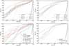 |
Fig. 2 Influence of the training data set for our baseline CNN (left, solid lines) and ResNet (right, dashed lines). We only vary the set of positive (top) and negative (bottom) examples. Networks trained on the baseline data sets (N1+L1) are plotted in dark blue. Two of the best networks from the upper-right panel, the baseline ResNet (N1+L1) and the ResNet from C21 (N1+L7), are shown as dashed gray lines in all panels for reference (except in the right-hand panels where the colors are overlaid by the ones indicated in the legend). The thick gray curve corresponds to a random classifier. Optimal performance is obtained for ground-truth data sets comprising mock lenses with bright, deblended multiple images, and large fractions of typical non-lens contaminants. The AUROC, TPR0 and TPR10 tend to be higher for the ResNet, except for data sets containing limited numbers of tricky non-lens galaxies. |
5.3 Network architectures
After characterizing the influence of the ground-truth data set, we used the baseline sets L1 and N1 to compare the performance of various network architectures. We tested several tens of network architectures obtained from variations of the baseline CNN, G-CNN and ResNet introduced in Section 4, in order to find the best network configurations for classifying small, ground-based lens image cutouts. Below, we highlight a representative subset of these tests, after excluding all architectures showing poor performance (AUROC ≲ 0.9). In particular, we start with a baseline (v1) for each of the CNN, G-CNN and ResNet as the reference architecture, and vary attributes such as the number of convolutional layers. We quantify the impact of these variations on the AUROC, TPR0 and TPR10, striving for architectures that maximize these metrics. The baseline model of each type serves only as a reference and does not need to be the optimal performing model.
The Convolutional neural networks (CNNs) are adapted from our baseline architecture that was previously applied to lens search in PanSTARRS multiband images (Cañameras et al. 2020). Apart from the items described below, all network parts are kept fixed to the baseline. To begin, CNN v2 adds a max-pooling layer after the third convolutional layer to further reduce the dimensions before flattening. CNN v3 includes a fourth convolutional layer with a kernel size of 5 × 5, while adapting the kernels of the first three layers to 11 × 11, 9 × 9, and 6 × 6. In contrary to v3, CNN v4 removes the third convolutional layer of the baseline architecture. Moreover, CNN v5 discards dropout regularization, CNN v6 only uses two FC hidden layers with larger number of neurons (1024 each), and CNN v7 uses batch normalization between each layer. Other architectures tested various number of filters in each convolutional layer, various position and number of max-pooling layers, or different number of neurons in the FC layers. We also tried to suppress all max-pooling layers, to move strides within the convolutional layers, and to change the kernel sizes in the max-pooling layers. These additional tests either showed minor differences from the baseline CNN or degraded the performance. Finally, varying dropout rates between 0.1 and 0.7 in steps of 0.1 gave similar results to dropout = 0.5.
The Residual neural networks (ResNets) are variations of the baseline architecture presented in Section 4, keeping a ResNet18-like structure with 8 blocks comprising two convolutional layers, batch normalization and ReLU activations. We successively modified different parts of the architecture to optimize the extraction of local spatial features, at the resolution of our seeing-limited images. ResNet v2 has a kernel of 5 × 5 pixels instead of 3 × 3 in the first convolutional layer before the residual blocks. ResNet v3 removes batch normalization after the first convolutional layer. ResNet v4 lowers the number of feature maps per group of two layers to 16, 32, 64, and 128. With respect to the baseline, ResNet v5 replaces the 2D average pooling with 2D maximal pooling layer before flattening. Moreover, ResNet v6 uses the lower number of filters of v4, while also removing the pooling layer and adding a new FC layer of 512 neurons. ResNet v7 sets stride = 1 instead of 2 in the second block and adds a FC layer of 128 neurons. Lastly, ResNet v8 tests the effect of applying dropout with rate of 0.5 before each FC layer.
The Group-equivariant neural networks (G-CNNs) correspond to three variants of the original G-CNN from Cohen & Welling (2016), which are better optimized for the small HSC image cutouts. G-CNN v1 has kernels of 7 × 7, 7 × 7, 5 × 5, and 3 × 3 pixels and 10, 10, 20, and 20 features maps per convolutional layer, and 64 neurons in the first FC layer before the single-neuron output layer. G-CNN v2 increases the number of feature maps to 20, 20, 40, and 40, and the number of neurons in the first FC layer to 128. G-CNN v3 is same as v1, but with 7 × 7 convolutions.
The performance with these various architectures are summarized in Figs. 3, 4 and Table 2. Overall, we obtain the best AUROC, TPR0, and TPR10 for the baseline ResNet. Such networks reaching the highest TPR0 = 30–40% are most useful to real lens searches in strongly unbalanced data sets, as they drastically limit the number of contaminants and save significant human inspection time. While only the baseline ResNet reach such elevated recall at zero contamination, all three G-CNNs and some of our CNNs and ResNets reach high TPR10 of about 50%.
In the literature, while ResNets have been often used for lens finding (e.g., Huang et al. 2021; Shu et al. 2022), their performance have been essentially evaluated on the Euclid lens-finding dataset (Metcalf et al. 2019). The ResNet from Lanusse et al. (2018) won the ground-based part of the challenge but Schaefer et al. (2018) found that deeper networks do not necessarily provide better performance. We can extend this comparison based on our new test sets drawn from real data and including representative populations of contaminants. Overall the best performance are obtained with ResNets but the improvement of ResNet architectures with respect to CNNs in terms of AUROC is clearly not systematic. Only the values of TPR0 tend to be higher for the ResNet (≃10–40%), with none of the CNN architecture we tested exceeding TPR0 ≃ 10%.
In particular, we find that CNNs with additional layers do not improve the classification. Using only two convolutional layers apparently degrades the performance (CNN v4), but we also noticed that changing the kernel size and lowering the number of filters allowed us to recover metrics similar to the baseline CNN. Moreover, our results show that fine-tuning the ResNet architecture helps improve the performance with respect to the original ResNet18. Optimizing the structure of the first layer in these ResNets to the size of input images appears to be particularly important given the lower AUROC and TPR0 in ResNets v2 and v3 with respect to the baseline. Similarly, varying the last FC layers has substantial impact (ResNets v7 and v8). The decrease in AUROC for ResNet v4 nonetheless shows that the number feature maps in the original ResNet18 architecture is well-suited for our classification problem. Finally, the three G-CNNs give remarkably stable performance in Table 2, as well as for alternative training sets, in agreement with the lower generalization gap observed in their loss curves compared to CNNs and ResNets.
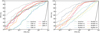 |
Fig. 3 Influence of the network architecture for our baseline data set and various CNNs (left) and ResNets (right). The baseline architectures are in dark blue. For reference, the dashed gray lines show two good networks (the baseline ResNet and the ResNet from C21). The thick gray curve corresponds to a random classifier. The best performance was obtained with the baseline ResNet. |
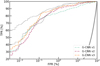 |
Fig. 4 Influence of the network architecture for our baseline data set and the group-equivariant network architectures G-CNNs adapted from Cohen & Welling (2016). For reference, the dashed gray lines show two good networks (the baseline ResNet and the ResNet from C21). The thick gray curve corresponds to a random classifier. |
Performance of various CNN and ResNet architectures.
5.4 Data processing
Image processing and image augmentation can affect the properties of the feature representation learned by the neural networks, thereby impacting their classification performance. For classification tasks working in meagre data regimes (e.g., radio galaxy classification, Aniyan & Thorat 2017; Slijepcevic et al. 2022), data augmentation is crucial in getting sizeable ground-truth data sets. In contrast, for strong-lens finding, we can rely on simulated training sets and use data augmentation to help models make stable predictions in the presence of perturbations on image centering and pixel intensity scaling. Here, we tested the impact of various data augmentation schemes using the baseline data set and the three gri-bands. The standard data processing recipe for both the baseline CNN and the baseline ResNet consists of applying random shifts sampled uniformly between −5 and +5 pixels to the image centroids, and taking the square root of pixel values (square-root scaling) after clipping negative pixels to zero. We demonstrate the importance of these two transformations in optimizing the performance, and we test a non-exhaustive list of additional data augmentation techniques.
Firstly, we evaluated the influence of centroid shifts, by training and testing on images perfectly centered on the relevant galaxy. The ROC curves in Fig. 5 show a significant drop in performance when removing the random shift in the image centroid. The AUROC of 0.9913 obtained for the baseline ResNet decreases to 0.8332 for this scenario, and both CNN and ResNet trained without random shifts have TPR0 of 0%. These results suggest that, in these cases, neural networks learn spatial offsets as a determinant feature for galaxy classification.
Secondly, we implemented different scaling and normalization schemes. To show the importance of applying a square-root scaling to individual images, we trained and tested the networks on original images from the baseline data set. The lower AUROC, TPR0, and TPR10 obtained for these networks with respect to the baseline (see Table 3) demonstrates the benefit of scaling the pixel values to boost the low-luminosity features and help learn the relevant information encoded in the lensed arcs. We tested other networks trained on alternative data sets from Section 3.1 and found systematically better performance with square-root scaling. On the contrary, using a log-scale or other approaches did not provide any improvement. A range of image normalization techniques were also tested such as scaling pixel values to the range 0–1, or normalizing images to zero mean and unit variance, and these techniques were applied either to individual images or to image batches. These processing methods were discarded from Fig. 5 as none of them reached performance comparable to the baseline networks.
Thirdly, we used various image rotation and mirroring, to help the networks learn invariance with respect to rotation and flipping operations. In the first version, we augmented the data set by loading the frames mirrored horizontally and vertically together with the original images, which resulted in three input images per object per band. In the second version, we applied random k × 90° rotations to each input object, while also loading the original and mirrored frames as described above. For the CNN, these approaches result in AUROC and TPR10 comparable to the baseline with a minor increase in TPR0 up to ≃5–10%. For the ResNet, performance are slightly lower than the baseline.
Fourthly, we tested using viewpoints (image crops) of the original images as input, following the general methodology employed in Dieleman et al. (2015) to reduce overfitting and improve rotation invariance for their galaxy morphological classifier. In the first version, we used four viewpoints of 40 × 40 pixels and random centers, corresponding to cropped version of the original images of 60 × 60 pixels in the baseline data set. Centroid positions were kept identical between bands. Depending on their position, these viewpoints cover either a fraction or the totality of the relevant lens systems and non-lens galaxies, and they have a significant mutual overlap. In that case, for a given entry in the data set, the neural networks were fed with a total of 12 input frames, corresponding to four viewpoints per band. In the second version, eight randomly centered viewpoints of 40 × 40 pixels were loaded, and we applied a random rotation by k × 90° to each viewpoint. In the third version, we also used eight viewpoints with random centroids and random rotations, but increased their size to 52 × 52 pixels. Given that our ResNet architectures are not adapted to these smaller crops, we only tested the extraction of viewpoints with the baseline CNN. Fig. 5 and Table 3 show that these approaches help boost the AUROCs, and interestingly, the TPR0 values are systematically higher than the baseline, and up to 17.5% for the first version.
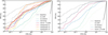 |
Fig. 5 Influence of the data augmentation procedure for our baseline data set, and for the baseline CNN (left, solid lines) and ResNet (right, dashed lines) architectures. The standard data processing plotted in dark blue consists of applying random shifts to the image centroids and square-root scaling (defined as “stretch” in the figure). The light green curves show networks trained without centroid shifts, and the dark green curves illustrate the performance without square-root scaling. The blue and brown curves correspond to networks trained on images loaded together with the frames mirrored horizontally and vertically, in each of the three gri-bands, with (brown) and without (blue) random rotations by k × π/2. The red, orange, and yellow curves in the left panel show the CNNs trained using viewpoints of the original images as inputs (see Section 5.4 for details). For reference, the dashed gray lines show two good networks (the baseline ResNet and the ResNet from C21). The thick gray curve corresponds to a random classifier. |
Tests of data processing and augmentation methods.
5.5 Number of observing bands
The influence of the observing bands was tested using the three gri-bands as baseline, and comparing with predictions obtained for combinations of one, two, or four bands. In HSC Wide, gribands have the best 5σ point-source sensitivities of 26.6, 26.2, and 26.2 mag, respectively (Aihara et al. 2019), together with a remarkably consistent depth between bands. The gri-bands will also be the deepest in the ten-year LSST stacks, about 1 mag deeper than HSC Wide according to the LSST baseline design (Ivezić et al. 2019). The z-band also considered in our analysis has a depth of 25.3 mag, and it will also be ≃1 mag shallower than gri in the final LSST stacks. For strong lenses, this redder band can play a role in identifying the signatures from the foreground galaxies with limited contamination from background lensed arcs that are mostly blue. In the LSST era, additional u-band images will reach similar depth as in the z-band, and they will play a role in identifying strong lenses. The results of our tests in Fig. 6 and Table 4 show that training the CNN jointly with the four bands helps boost the AUROC, TPR0, and TPR10 compared to the baseline CNN trained on gri. Interestingly, training either with gi- or gz-bands gives better performance than gri, with the highest TPR0 of 30.7% obtained with gz-bands. This could either be due to different image resolutions per band (see Section 6) or fluctuations in TPR0 due to the moderate number of test lenses. Other combinations of two bands give either poor AUROC ≃ 0.93 or very low recall at zero contamination. Lastly, training with one band performs much worse, with the highest AUROC obtained for the i-band, and none of the single-band networks providing high enough TPR10 ≥ 10%.
5.6 Data set size
The ideal size of the ground-truth data set depend both on the network depth and size of input images. While classical CNNs with only a couple of convolutional layers show stable performances for training sets with ≥105 images (e.g., He et al. 2020), the classification accuracies for smaller sets down to ≃104 examples deserve further tests, in particular for deeper ResNet architectures. We characterized the influence of the data set size by training and validating our CNN and ResNet on different fractions of the overall baseline data set. We used between 10% and 100% of all images, in steps of 10%, or between 7000 and 70 000 training examples. Table 5 (and Fig. 7) show that AUROCs do not smoothly increase as a function of the data set size. This is likely due to the combined effect of (1) the different training set content, (2) the stochasticity of the learning process, and (3) the finite size of our set of test lenses causing small fluctuations in TPR0 and TPR10.
The results are more stable for CNNs that have AUROC in the range 0.9426–0.9806, TPR0 ≃ 0%, and TPR10 ≃ 30–50%. The CNN with highest AUROC uses only 10% of the data set, suggesting that ≃104 examples is sufficient to train shallow networks. Many ResNets have better performance than the CNNs, with AUROC up to 0.9913 and zero-contamination recall up to 36.0% for the ResNet using the entire data set, but the scatter is also larger (e.g. AUROC of 0.8583 for a fraction of 50%). In contrast to CNNs, the ResNets tend to show an improvement in performance as a function of the number of training examples (see Table. 5). This trend is most prominent for the TPR0 values that increase from 3.7–16.4% for fractions ≤50% to 8.5–36.0% for fractions >50%.
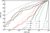 |
Fig. 6 Receiver operating characteristic curves for training with different numbers of observing bands for the baseline CNN and the training set. For reference, the dashed gray lines show two good networks (the baseline ResNet and the ResNet from C21). The thick gray curve corresponds to a random classifier. Adding z-band to the standard gri three-band input helps increase the AUROC. |
Performance as a function of the number of observing bands.
Performance for various fractions of the overall data set.
5.7 Difference images
The populations of lens and source galaxies targeted by our overall search experiment show a strong color dichotomy. As we specifically focus on foreground galaxies with the highest lensing cross-section, samples of lens galaxies are dominated by massive early-type galaxies with red colors and smooth light profiles. For deep, ground-based imaging surveys, typical galaxies magnified by these light deflectors are located at z = 1–4, an epoch dominated by bluer star-forming galaxies. For galaxy-scale systems, the signals from both components are necessarily blended to some extents. To help the networks access the signal from the lensed arcs, we attempted using difference images (DI) obtained from the subtraction of the red i-band from the blue g-band frames. The subtraction g – αi includes a rescaling term α computed as follows:
 (2)
(2)
where cModel are the composite model magnitudes obtained from the combined fit of exponential and de Vaucouleurs profiles (Lupton et al. 2001; Bosch et al. 2018). Because it is based on the cModel photometry, a accounts for the PSF FWHM in each band. To compute the difference image of each object in the baseline data set and in the test set, we used the cModel magnitudes listed in the HSC PDR2 tables. This approach only considers the central object, and difference images of the mocks were thus obtained using the photometry of the lens galaxy without arc-light contamination. For mocks in the baseline data set, Fig. 8 shows that difference images efficiently remove the lens light and help emphasize the signatures from background sources. The PSF FWHM of g- and i-band images were not matched to avoid convolution overheads and, in consequence, the central emission is oversubtracted. This artifact is mitigated by the clipping of negative pixels included in our data loader.
Figure 9 and Table 6 show the results of training the networks on the difference images alone, or after combining these frames with original images in i-band, which has the best seeing, or with the three gri-bands. We find poor classifications for networks trained, validated, and tested only with difference images due to the lack of signal from the lens galaxy and companions, residuals from differences in g- and i-band seeing, or both effects. Other approaches depend on the architecture. For the CNN, we obtain higher AUROC, TPR0, and TPR10 when using DI + gri-bands compared to the baseline. This suggests that adding input frames with clearer signal from the lensed arcs help slightly improve the recall of SuGOHI lenses. However, this gain disappears for the ResNet.
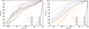 |
Fig. 7 Receiver operating characteristic curves for training with different fractions of the overall data set, for the baseline training set and for the baseline CNN (left) and ResNet (right). For reference, the dashed gray lines show two networks among the best networks from Fig. 2 (the baseline ResNet and the ResNet from C21). The thick gray curve corresponds to a random classifier. |
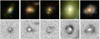 |
Fig. 8 Mosaic of difference images for mocks in the baseline data set. Top: three-color images from the original gri stacks. Bottom: corresponding difference images based on a simple subtraction of the rescaled i-band from the g-band frames. |
5.8 Masking neighbors
Our classification experiments include neighboring galaxies in the 10″ × 10″ HSC cutouts around the central galaxy or strong-lens system tabulated in our data sets. Neural networks learn the status of these nearby, unassociated galaxies during the training phase. We tried to mask the neighboring sources as part of the preprocessing of images in the training, validation, and test sets, to determine whether or not this helps the networks focus on the relevant sources and improve their performance. We used SExtractor (Bertin & Arnouts 1996) to mask galaxies that are deblended well from the central objects, which were required to be within five pixels from the cutout centers. A low number of deblending thresholds, DEBLEND_NTHRESH of 16 and a contrast parameter, DEBLEND_MINCONT of 0.01 were chosen to avoid identifying local peaks in the light distributions. We defined the masks in r-band, using the 3σ isophotes after convolving the images by Gaussian kernels with FWHM of 2 pixels. This optimal tradeoff provided adequate deblending in all three gri-bands, while smoothing the mask edges, and keeping features near the central galaxy (e.g. lensed arcs) within the masks. In some cases, interesting features were inevitably masked out with this automated procedure. We nonetheless noticed that all multiple lensed images were within the masks for nearly all SuG-OHI test lenses, and all strong-lens simulations with θE ≲ 2.0″. The lensed arcs with largest separation from the lens center were masked out for only ≃10% of mocks with θE > 2.0″.
The results in Fig. 9 and Table 6 indicate that the masking procedure improves the metrics for the CNN, but not for the ResNet. For the CNN, we obtain a substantial increase in AUROC to 0.9949, which is the highest AUROC over all tests conducted in this study, and we get a TPR10 of 50% approaching the recall of the baseline ResNet. For the ResNet, the lower performance compared to the baseline might suggest that artifacts from the masking procedure (e.g., sharp mask edges, truncated galaxy light profiles) inevitably affect the underlying model.
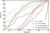 |
Fig. 9 Performance of networks trained, validated and tested on difference images g – αi alone (red), joined with images from the i-band that has the best seeing (brown), or joined with the three gri-bands (orange). Blue curves show the baseline CNN (solid) and ResNet (dashed) trained, validated and tested on gri images with neighboring galaxies masked (see Section 5.8). For reference, the dashed gray lines show two good networks (the baseline ResNet and the ResNet from C21). The thick gray curve corresponds to a random classifier. We obtain a significant improvement in AUROC for the CNN after masking companions galaxies. |
5.9 Number of output classes
To assess the influence of the number of ouput classes in the neural networks used for our classifications, we tested the baseline CNN and ResNet architectures with four classes instead of two.
The data set was kept similar to the baseline, with the first class including the baseline mocks from set L1, and the three other classes containing LRGs, spirals, and random galaxies, respectively, selected in the same way as for set N1. Given the moderate number of compact groups in our parent sample, this type of non-lens galaxies was discarded from this test. The number of elements per class was kept balanced to 24 500 examples, and architectures matched the baseline CNN and ResNet apart from the four-neuron output layer. We determined the performance of this multiclass classification using the ROC curves of class “lens”. For the CNN, we obtain AUROC, TPR0, and TPR10 of 0.9808, 12.2%, and 33.3%, respectively, while for the ResNet we find an AUROC of 0.9824, a TPR0 of 9.0%, and a TPR10 of 31.8%. Compared to binary classification, the CNN reaches higher AUROC and TPR0 but lower TPR10, and the performance globally decreases for the ResNet.
Performance of networks using difference images.
5.10 Committees of networks
Ensemble learning refers to training multiple neural networks for the same task and combining predictions from the ensemble of models. This method has proven helpful to mitigating the stochasticity of the learning process, and to lower the generalization error and variance in output scores (Hansen & Salamon 1990; Krogh & Vedelsby 1994). We applied this approach to our binary classification problem, first by training a committee of five networks with fixed architecture, ground-truth dataset and dataset split, but with different weight initialization (e.g., Schaefer et al. 2018). Secondly, we trained five networks with fixed architecture and ground-truth data, but with random split into training and validation, and with different random initialization of the networks weights. In both cases, the procedure was repeated for the CNN and ResNet. Thirdly, we used committees of the best networks from Table 1 trained on different ground-truth data sets (see Section 5.2). The output scores of the network committees were then averaged to obtain the final prediction. Other combinations of scores, for instance by taking the median, minimal, or maximal value over the five models, did not improve the performance.
Figure 10 and Table 7 show that the third approach gives the most significant boost in performance. While averaging scores from random networks in Table 1 does not systematically improve the overall metrics, selecting the networks with good performance and different internal representations turns out to be more useful. To identify the best networks to combine, we selected the 10 networks with highest AUROC in Table 1, and we counted the number of false positives and false negatives overlapping between pairs of networks. For that, we first selected for each network the 50 SuGOHI lenses with lowest scores and found that the overlap between pairs of networks varied between 30 and 40 objects. We then identified for each network the 50 non-lenses in COSMOS with highest scores and found that networks tend to be contaminated by different false positives, with only about 3–15 objects in common between pairs of networks. Given the higher overlap between false negatives found by each network than between false positives, we averaged the scores from the networks with the lowest number of false positives in common. We obtained the most significant improvement by combining the baseline ResNet, the ResNet trained on sets L4 and N1, and the ResNet from C21 trained on L7 and N1 (see Fig. 10). This committee reaches the highest TPR0 and TPR10 over our various tests, and obtaining a recall at zero contamination as high as ≃60% opens promising perspectives for pure selection of strong lenses without human input. Regarding the first two approaches, Table 7 shows a significant improvement of each metric for the CNN (as also found by Schaefer et al. 2018), but lower performance for the ResNet.
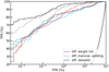 |
Fig. 10 Performance of committees of networks. The red curves show the committee of five networks with different weight initialization. The blue curves instead use fixed architecture and ground-truth data, but random split into training and validation, and different weight initialization. Black curves show a committee of networks trained on different data sets (see Section 5.10). As in previous plots, solid and dashed lines correspond to the CNN and ResNet architectures, respectively. The third approach gives the most significant boost in performance and allowed us to overcome the AUROC, TPR0 and TPR10 of the best individual networks shown as gray lines (the baseline ResNet and the ResNet from C21 |
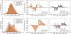 |
Fig. 11 Histograms of seeing FWHM difference between pairs of bands. In the left panels, gray histograms show the average distributions over the entire HSC PDR2 footprint, and orange filled histograms show the distributions restricted to the GAMA09H field. In addition, step histograms show the distributions for galaxies within GAMA09H assigned the 1% highest scores by the ResNet from C21. In the middle panels, orange curves show the excess of the 1% top scores, obtained from the bin-per-bin difference between the step and filled orange histograms in the left panel. Other curves in the middle and right panels show this excess distribution for other networks. |
Performance of committees of networks.
6 Discussion
After comparing the performance of various networks using fixed test sets, we explore potential biases in the network predictions. Two main effects have been identified as part of our study of the relationship between output scores and observational parameters, or image properties. First, we investigate in Section 6.1 a dependence of network scores on image quality, and second, in Section 6.2, we address a dependence on image orientation. In Section 6.3, we evaluate the properties of SuGOHI test lenses correctly and incorrectly classified by the best networks from Section 5.
6.1 Dependence on local seeing
In the Wide HSC layer, the excellent i-band seeing required for weak-lensing analyses results in significant differences with other bands. Training our supervised neural networks on these multiband images without matching the PSF per band can introduce dependencies on systematic variations in seeing FWHM (see also Li et al. 2021). In our experiments, all training images were distributed randomly over the PDR2 footprint and, for the lens simulations, local PSF models were used to paint lensed arcs with realistic angular resolutions. Although this procedure guarantees that the network inputs account for variations in image quality, it does not rule out biases in the output scores as a function of local seeing FWHMs.
To probe the dependence on the gri-band seeing, we used the GAMA09H field that shows the largest differences in seeing distributions compared to the overall footprint. The difference in seeing FWHM between pairs of bands are plotted in Fig. 11 and show a good match for g–i, but a major secondary peak in GAMA09H for the r–i distribution. This peak corresponds to locations where the r- and i-band seeing are anticorrelated with broader light profiles in r-band. In these cases, isolated LRGs appear surrounded by bluer halos due to the PSF mismatch, an artifact that closely mimics strongly lensed images blended with a central deflector. Unsurprisingly, by plotting the 1% galaxies in GAMA09H obtaining highest network scores (see Fig. 11), it appears that predictions from the ResNet of C21 heavily depend on the local seeing values. The significant excess of strong-lens candidates identified by this network for r–i FWHM above 0.4″ (compared to the distribution over the entire footprint) suggests that the underlying model tends to identify color gradients in the galaxy light profiles as lensed arcs. The baseline ResNet shows a similar distribution as the C21 ResNet, with a deficit and excess of high scores for r–i FWHMs below and above 0.4″, respectively. For the baseline ResNet, the bimodal trend also appears in the difference between g- and i-band seeing FWHMs. The baseline CNN exhibits a similar bimodality but with lower amplitude in both pairs of bands.
We investigated various methods to reduce this bimodality and obtain invariance to seeing FWHMs. A significant improvement was found by simply adding the z-band as fourth frame to the network inputs, as shown in Fig. 11 (right panel) for the baseline CNN architecture. The median seeing of 0.68″ in z-band is intermediate between the median values in i-band (0.58″) and gr-bands (≃0.76″), providing a straightforward way to help the networks classify color gradients as observational artifacts. Furthermore, providing the PSF cutouts as inputs together with the gri science frames also prove successful in removing the bimodality. This technique was previously used in supervised neural networks, for instance for estimating galaxy structural parameters (Li et al. 2022). In our case, we used the baseline ground-truth data set and we imported the HSC PDR2 PSF at the position of the central galaxy in each cutout. Zero-padding pixels were added to the 42 × 42 pixels PSF frames to match the dimension of science images. We then used our baseline architectures to train a CNN and a ResNet using a six-dimension input with the gri coadds and corresponding PSF frames. After appending the PSF frames to our test set we find AUROC, TPR0, and TPR10 of 0.9716, 23.8, and 46.6% for the CNN, comparable to our best networks and plotted in Fig. 11, and 0.9375, 22.8, and 32.3% for the ResNet, respectively. Other alternatives would be to apply random gaussian blurring as Stein et al. (2022), or to provide PSF FWHMs as numerical inputs before the FC layers, similarly to the combination of morphological parameters and multiband images used by Pearson et al. (2022) for their searches for galaxy mergers. Both approaches were discarded since the extra blur affected the recall of small-separation SuGOHI lenses, and we could not obtain competitive performance for CNNs and ResNets combining image and catalog input.
6.2 Dependence on image rotation
The variations of network output scores as a function of image orientation were characterized by classifying original HSC cutouts and cutouts rotated by k × π/2, where k = 0,1,2,3, for the 189 SuGOHI lenses in our test set. Our neural networks tend to provide classifications that are nearly invariant to image orientation for objects identified as clear lenses (mean scores μp ≃ 1) and clear non-lenses (mean scores μp ≃ 0). For instance, we find that predictions with a mean score μp < 0.1 or > 0.9 over the four image orientations, systematically have a low average scatter σp ≲ 0.02 for the baseline CNN, the baseline ResNet, and the ResNet from C21.
SuGOHI lenses with intermediate mean scores are much more sensitive to the orientation of input frames. For lenses with a mean network score μp in the range 0.1–0.9, we find a scatter σp ≃ 0.18, 0.21, and 0.16 with the baseline CNN, the baseline ResNet, and the ResNet from C21, respectively. Using G-CNN architectures allows this dependence to be significantly lower. For instance, with the G-CNN v3 that showed the highest AUROC over the three architectures we tested, the scatter decreases to σp ≃ 0.08. While G-CNNs are built to achieve rotation invariance, the scatter for G-CNNs does not decrease to zero due to the additional effect from the random centering offsets applied to images prior to classification (see Section 5.4).
6.3 Properties of false negatives and false positives
As noted in Section 5.10, there is a substantial overlap between the SuGOHI lenses assigned low scores by different neural networks. In Fig. 12, we compare the properties of test lenses that are recovered or missed by a representative selection of seven high-performing networks. These distributions are plotted for fiducial score thresholds resulting in a common recall of 50%. For each SuGOHI system, the cModel magnitudes, the Kron radius, and the photometric redshift (from the Mizuki template-fitting code of Tanaka 2015) of the foreground lens galaxy were retrieved from the pdr2_wide.forced and pdr2_wide.photoz_mizuki tables. We also relied on the strong-lens modeling neural network from Schuldt et al. (2023a) to obtain the SIE parameters and external shear for all lenses in this test set. The subset of 30 SuGOHI systems with ancillary Markov-Chain Monte-Carlo sampling-based models shows good agreement between both Einstein radius estimates, with the distribution in ΔθE having median and 1σ ranges of  (see Schuldt et al. 2023b, for a detailed comparison of modeling approaches).
Figure 12 shows that networks miss the majority of lenses with faint deflectors having i ≃ 21–22 mag. These networks are trained on various sets of mocks produced from the same parent sample of LRGs with zspec and vdisp measurements. In consequence, while the icModel distributions for the mocks and SuGOHI sample both peak at ≃19–20 mag, all i > 21 mag deflectors without SDSS spectroscopy follow-up are discarded from training. The lens (g – i) colors do not have such a discrepancy between the training and test lenses. The recall is roughly constant as a function of lens color, apart from the tail of bluer lens galaxies with (g – i) ≲ 2, which have a lower recall in four out of seven networks. In terms of lens zphot, we also obtain a stable recall up to the highest lens redshifts of zphot ≳ 0.7. This stability was however only reached after boosting the fraction of lens LRGs with zphot above the peak of the SDSS sample in our various training sets. The baseline CNN is the network showing the most significant drop in recall at zphot ≃ 0.5. The distributions of lens i-band Kron radii have stronger differences, especially at the high end > 1.3″, where the majority of lenses are missed by all seven networks. In contrast to i-band magnitudes, this bias results from the acceptance criteria of simulated arcs rather than properties of the parent LRG sample. Besides excluding mocks with multiple images buried in lens light, the Rsr/ls.min threshold also tends to discard the extended LRGs that dominate over lensed source emission for any value of μ. This explains the failure in identifying this subset of SuGOHI lenses. Since our aim is to have good overall recall on the full sample of SuGOHI, we do not further optimize the network for such a specific subset and we avoid overfitting to the subset.
The recall of SuGOHI lenses strongly varies with Einstein radius. Even though simulations for training the baseline networks and the ResNet of C21 cover the entire 0.75–2.5″ range uniformly, the recall at θE ≲ 1.2″ is < 15%. The recovery of wider image separation systems is higher, but still incomplete. Fig. 12 also includes networks trained on natural θE distribution, and on uniform distributions with θE ≥ 1″ and θE < 2″. These networks do not succeed in extracting blended lensed arc features, but we nonetheless notice an influence from the relative fraction of compact and extended image configurations in the training sets, as the recall at θE < 1.2″ increases for the ResNet trained mostly on low-θE mocks. Interestingly, the recall at small θE does not improve significantly for the network trained on difference images (not shown in Fig. 12).
We also classified the SuGOHI colors visually to assign a “red” flag to sources redder than the lens galaxy. We find that the test sample is strongly dominated by blue lensed sources, with only 10 sources marked as “red”. Despite our efforts in extending the source color distribution in the training sets, we find that the recall of red SuGOHI arcs remains low. Only the baseline ResNet, the ResNet trained on sets N1+L4, and the CNN trained on four bands are able to find three or four of these 10 sources, while other networks miss them all. This matches results for other lens-finders (e.g., Jacobs et al. 2022).
Overall, test lenses that are incorrectly classified for the fiducial score thresholds adopted in this section, tend to have properties deviating from the bulk of the mocks in the training sets (see e.g., Fig. 13 for the baseline ResNet). This common behavior for supervised machine learning algorithms can be corrected by expanding the parameter space covered by the simulations. In the future, deeper spectroscopic surveys will help in that regard, as they will provide more diverse lens and source samples for our simulation pipeline. Regarding false positives, we found that high-performing networks are contaminated by diverse, mostly distinct galaxy types. Only a few of them show apparent arc-like features, and the majority belong to morphological classes relatively less represented in our ground-truth data, such as galaxies with dust lanes, or edge-on disks. Finally, contaminants do not follow obvious trends with structural parameters.
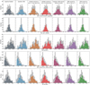 |
Fig. 12 Properties of SuGOHI lenses in our test set that are recovered (plain) or missed (steps) by our networks, for fiducial score thresholds resulting in 50% recall. The histograms for all SuGOHI lenses are plotted in light gray. From left to right, we show the baseline ResNet, the baseline CNN, the ResNet trained on sets N1+L7 (network used in C21the ResNet trained on sets N1+L4 (natural θE distribution), the baseline CNN trained on griz-bands instead of gri, the CNN trained on sets N1+L2 (θE ≥ 1″), and the CNN trained on sets N1+L3 (θE < 2″). |
7 Summary
We have conducted a systematic comparison of supervised neural networks for selecting galaxy-scale strong gravitational lenses in ground-based imaging. Identifying the main ingredients to optimize the classification performance of these networks is becoming crucial to reduce the contamination rates and the need for human resources. We used PDR2 images from the HSC Wide survey to address this issue and to prepare for the exploitation of forthcoming deep, wide-scale surveys such as Rubin LSST. A representative test set was designed with 189 strong lenses previously found in HSC and 70 910 non-lens galaxies in the COSMOS field, including a realistic number and diversity of lens-like galaxies, in order to mimic an actual classification set up. Multiple networks were trained on different sets of realistic strong-lens simulations and non-lens galaxies, with various architectures and data preprocessing, and mainly using the gri-bands that have optimal depth. These networks reached an excellent AUROC on the test set, but the recall for zero and ten false positives showed wide ranges of values. The following conclusions have been drawn:
As expected, choices in the construction of the ground-truth training data have a major impact. Optimal performance is only obtained for data sets comprising mock lenses with bright, deblended multiple images and including boosted fractions of non-lens contaminants. The AUROC, TPR0, and TPR10 are typically (but not systematically) higher for the baseline ResNet. The metrics are less affected by changes in the ground-truth data for the baseline CNN.
The best performance are obtained for the baseline ResNet which is adapted from ResNet18. We explored variations around the baseline CNN, ResNet, and G-CNN architectures, finding that while some CNNs perform better than ResNets, the TPR0 tends to be higher for ResNets (≃ 10–40%), with none of the CNNs exceeding TPR0 ≃ 10%.
We have tested a variety of data preprocessing and find that the random shifts to the image centroids and square-root scaling of the pixel values give systematic improvements in the performances of the networks. Simple augmentation procedures, such as loading the frames mirrored horizontally and vertically together with the original images, help increase the recall at low contamination for the CNN, but not for the ResNet. For CNNs, using random viewpoints of the original images as input also provide an additional gain compared to using 10″ × 10″ gri stacks. We also find an improvement when adding the z-band to gri.
The CNN shows a more stable performance than the ResNet as a function of training set size when varying between 7000 and 70 000 examples. The metrics, TPR0 in particular, raise significantly for the ResNet when increasing the number of training examples.
Using g – αi difference images to subtract emission from the main central galaxy does not improve the classification, likely due to the differences in g- and i-band seeing. However, we find that masking neighboring galaxies leads to a major gain in AUROC for the CNN.
Using committees of networks trained on different data sets, and with the lowest overlap in false positives, turns out to provide the most significant gain in performance. This results in the highest TPR0 and TPR10 over our various tests of about 60 and 80%, respectively. In addition, using committees of networks with different weight initialization does not provide such gain but helps stabilize the metrics compared to individual networks.
Moreover, despite using accurate PSF models in the lens simulations, some networks show systematic dependence with variations in seeing FWHM (see Section 6.1) and image depth (see Appendix) between observing bands over the footprint. For our baseline networks trained on gri-bands, dependencies on image quality are particularly important over regions where the r- and i-band seeing are anticorrelated, with broader light profiles in the r-band. The underlying models tend to associate such color gradients produced by the PSF mismatch with genuine strong-lensing features, leading to an excess of spurious strong-lens candidates. We investigated various methods to obtain invariance to seeing FWHMs and found excellent improvement when training either with the four griz-bands or with gri science frames together with the corresponding PSF cutouts. This illustrates that specific strategies are needed to ensure neural networks correctly account for observational effects in their underlying models.
Overall, the systematic tests presented in this paper demonstrate a feasibility of reaching a recall as high as 60% with zero contamination, which opens promising perspectives for pure selection of strong lenses without human input or with only modest human input. The conclusions drawn from this analysis are necessarily affected by the construction of our test sets and the potential fluctuations in TPR0 given the finite sample size, and they are mostly valid for bright lens samples (r < 21), while fainter systems would just degrade the performances of the algorithms. We nonetheless expect that the main results will hold for next-generation ground-based surveys with comparable image depth and quality, such as Rubin LSST. Together with new strong-lens simulations matching the image quality of these forthcoming surveys and with extensive tests of the network selection functions (e.g., More et al. 2024), these ingredients will allow optimal classification performance to be reached.
In the future, one priority will be to increase the recall of strong lenses with broader types of lens potentials, including exotic systems that are more difficult to mock up (see, e.g., Wilde et al. 2022), while maintaining low contamination rates. This could be done via novel approaches, such as combinations of unsupervised and supervised machine learning methods or anomaly detection algorithms. Storey-Fisher et al. (2021) explored anomaly detection in the same HSC data set by training a generative adversarial network on HSC Wide PDR2 multiband images. While 4500 out of their 13 000 high-anomaly objects are included in our parent sample of galaxies with Kron radius ≥0.8″, only a handful are flagged as strong-lens candidates in C21, likely due to diffraction spikes from nearby stars ratherthan the presence of lensed arcs. Further work is therefore needed to identify the rare strong gravitational lenses as systems deviating significantly from standard morphological classes.
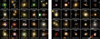 |
Fig. 13 Examples of 20 SuGOHI lenses recovered (left) and missed (right) by our baseline ResNet ranked by increasing network scores. |
Acknowledgements
We thank the referee for the detailed comments that helped improve the quality and clarity of the paper. R.C. and S.H.S. thank the Max Planck Society for support through the Max Planck Research Group for S.H.S. This project has received funding from the European Research Council (ERC) under the European Union’s Horizon 2020 research and innovation program (LENSNOVA: grant agreement No 771776). This research is supported in part by the Excellence Cluster ORIGINS which is funded by the Deutsche Forschungsgemeinschaft (DFG, German Research Foundation) under Germany’s Excellence Strategy – EXC-2094 – 390783311. S.S. has received funding from the European Union’s Horizon 2022 research and innovation programme under the Marie Skłodowska-Curie grant agreement No 101105167 — FASTIDIoUS. S.B. acknowledges the funding provided by the Alexander von Humboldt Foundation. A.T.J. is supported by the Program Riset Unggulan Pusat dan Pusat Penelitian (RU3P) of LPIT Insitut Teknologi Bandung 2023. This paper is based on data collected at the Subaru Telescope and retrieved from the HSC data archive system, which is operated by Subaru Telescope and Astronomy Data Center at National Astronomical Observatory of Japan. The Hyper Suprime-Cam (HSC) collaboration includes the astronomical communities of Japan and Taiwan, and Princeton University. The HSC instrumentation and software were developed by the National Astronomical Observatory of Japan (NAOJ), the Kavli Institute for the Physics and Mathematics of the Universe (Kavli IPMU), the University of Tokyo, the High Energy Accelerator Research Organization (KEK), the Academia Sinica Institute for Astronomy and Astrophysics in Taiwan (ASIAA), and Princeton University. Funding was contributed by the FIRST program from Japanese Cabinet Office, the Ministry of Education, Culture, Sports, Science and Technology (MEXT), the Japan Society for the Promotion of Science (JSPS), Japan Science and Technology Agency (JST), the Toray Science Foundation, NAOJ, Kavli IPMU, KEK, ASIAA, and Princeton University. This paper makes use of software developed for the LSST. We thank the LSST Project for making their code available as free software at http://dm.lsst.org. This work uses the following software packages: Astropy (Astropy Collaboration 2018), matplotlib (Hunter 2007), NumPy (Harris et al. 2020), Scipy (Virtanen et al. 2020), torch (Paszke et al. 2019).
Appendix A Dependence on image depth
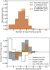 |
Fig. A.1 Histograms of the number of frames per stack in g-band. In the top panel, the gray histogram shows the average distributions over the entire HSC PDR2 footprint, and the orange filled histogram shows the distributions restricted to the GAMA09H field. In addition, the step histogram shows the distributions for galaxies within GAMA09H assigned the 1% highest scores by the ResNet from C21. In the bottom panels, orange curves show the excess of the 1% top scores, obtained from the difference between the step and filled orange histograms in the top panels, and other curves showing additional networks. |
Taking advantage of the on-going status of the HSC Wide survey, we characterized the variations of output scores as a function of image depth. For each band, the number of frames per stack was used as proxy of depth5 and we compared the distributions for galaxies over the overall footprint, within GAMA09H, and with the 1% highest scores for various networks in Fig. A.1, A.2, and A.3. While the C21 ResNet remains relatively invariant to the number of frames, the highest scores identified by the baseline CNN shows a strong excess of galaxies with ≤3 frames per stack in all three bands, suggesting that its predictions are biased for the shallowest images. The baseline ResNet shows the opposite trend in g- and r-bands, with a deficit and excess of high scores for ≤4 and >4 frames, respectively. As previously, adding z-band as input appears to naturally avoid biased predictions for galaxies without full-depth observations in gri-bands. More homogeneous coverage in later HSC releases and dedicated observing strategies for Rubin LSST will also help mitigate such biases in the future.
References
- Abolfathi, B., Aguado, D. S., Aguilar, G., et al. 2018, ApJS, 235, 42 [NASA ADS] [CrossRef] [Google Scholar]
- Aihara, H., Arimoto, N., Armstrong, R., et al. 2018a, PASJ, 70, S4 [NASA ADS] [Google Scholar]
- Aihara, H., Armstrong, R., Bickerton, S., et al. 2018b, PASJ, 70, S8 [NASA ADS] [Google Scholar]
- Aihara, H., AlSayyad, Y., Ando, M., et al. 2019, PASJ, 106, 12 [Google Scholar]
- Aniyan, A. K., & Thorat, K. 2017, ApJS, 230, 20 [Google Scholar]
- Astropy Collaboration (Price-Whelan, A.M., et al.) 2018, AJ, 156, 123 [NASA ADS] [CrossRef] [Google Scholar]
- Bautista, J. E., Vargas-Magaña, M., Dawson, K. S., et al. 2018, ApJ, 863, 110 [NASA ADS] [CrossRef] [Google Scholar]
- Beckwith, S. V. W., Stiavelli, M., Koekemoer, A. M., et al. 2006, AJ, 132, 1729 [Google Scholar]
- Bertin, E., & Arnouts, S. 1996, A&AS, 117, 393 [NASA ADS] [CrossRef] [EDP Sciences] [Google Scholar]
- Bolton, A. S., Burles, S., Koopmans, L. V. E., et al. 2008, ApJ, 682, 964 [Google Scholar]
- Bonvin, V., Courbin, F., Suyu, S. H., et al. 2017, MNRAS, 465, 4914 [NASA ADS] [CrossRef] [Google Scholar]
- Bosch, J., Armstrong, R., Bickerton, S., et al. 2018, PASJ, 70, S5 [Google Scholar]
- Brownstein, J. R., Bolton, A. S., Schlegel, D. J., et al. 2012, ApJ, 744, 41 [NASA ADS] [CrossRef] [Google Scholar]
- Cañameras, R., Schuldt, S., Suyu, S. H., et al. 2020, A&A, 644, A163 [Google Scholar]
- Cañameras, R., Schuldt, S., Shu, Y., et al. 2021, A&A, 653, L6 [NASA ADS] [CrossRef] [EDP Sciences] [Google Scholar]
- Chan, J. H. H., Suyu, S. H., Sonnenfeld, A., et al. 2020, A&A, 636, A87 [NASA ADS] [CrossRef] [EDP Sciences] [Google Scholar]
- Cheng, T.-Y., Li, N., Conselice, C. J., et al. 2020, MNRAS, 494, 3750 [NASA ADS] [CrossRef] [Google Scholar]
- Cheng, T.-Y., Huertas-Company, M., Conselice, C. J., et al. 2021, MNRAS, 503, 4446 [NASA ADS] [CrossRef] [Google Scholar]
- Cohen, T. S., & Welling, M. 2016, arXiv e-prints [arXiv:1602.07576] [Google Scholar]
- Collett, T. E. 2015, ApJ, 811, 20 [NASA ADS] [CrossRef] [Google Scholar]
- Craig, P., O’Connor, K., Chakrabarti, S., et al. 2024, MNRAS, 534, 1077 [NASA ADS] [CrossRef] [Google Scholar]
- Diehl, H. T., Buckley-Geer, E. J., Lindgren, K. A., et al. 2017, ApJS, 232, 15 [NASA ADS] [CrossRef] [Google Scholar]
- Dieleman, S., Willett, K. W., & Dambre, J. 2015, MNRAS, 450, 1441 [NASA ADS] [CrossRef] [Google Scholar]
- D’Isanto, A., & Polsterer, K.L. 2018, A&A, 609, A111 [NASA ADS] [CrossRef] [EDP Sciences] [Google Scholar]
- Faure, C., Kneib, J.-P., Covone, G., et al. 2008, ApJS, 176, 19 [NASA ADS] [CrossRef] [Google Scholar]
- Gavazzi, R., Marshall, P. J., Treu, T., & Sonnenfeld, A. 2014, ApJ, 785, 144 [Google Scholar]
- Goldstein, D. A., & Nugent, P. E. 2017, ApJ, 834, L5 [Google Scholar]
- Goldstein, D. A., Nugent, P. E., & Goobar, A. 2019, ApJS, 243, 6 [NASA ADS] [CrossRef] [Google Scholar]
- Gong, Y., Liu, X., Cao, Y., et al. 2019, ApJ, 883, 203 [NASA ADS] [CrossRef] [Google Scholar]
- Green, J., Schechter, P., Baltay, C., et al. 2012, arXiv e-prints [arXiv:1208.4012] [Google Scholar]
- Hansen, L., & Salamon, P. 1990, IEEE Trans. Pattern Anal. Mach. Intell., 12, 993 [CrossRef] [Google Scholar]
- Harris, C. R., Millman, K. J., van der Walt, S. J., et al. 2020, Nature, 585, 357 [NASA ADS] [CrossRef] [Google Scholar]
- He, K., Zhang, X., Ren, S., & Sun, J. 2016, arXiv e-prints [arXiv:1603.05027] [Google Scholar]
- He, Z., Er, X., Long, Q., et al. 2020, MNRAS, 497, 556 [NASA ADS] [CrossRef] [Google Scholar]
- Hezaveh, Y. D., Perreault Levasseur, L., & Marshall, P. J. 2017, Nature, 548, 555 [Google Scholar]
- Hocking, A., Geach, J. E., Sun, Y., & Davey, N. 2018, MNRAS, 473, 1108 [CrossRef] [Google Scholar]
- Huang, X., Storfer, C., Gu, A., et al. 2021, ApJ, 909, 27 [NASA ADS] [CrossRef] [Google Scholar]
- Hunter, J. D. 2007, Comput. Sci. Eng., 9, 90 [NASA ADS] [CrossRef] [Google Scholar]
- Inami, H., Bacon, R., Brinchmann, J., et al. 2017, A&A, 608, A2 [NASA ADS] [CrossRef] [EDP Sciences] [Google Scholar]
- Ioffe, S., & Szegedy, C. 2015, Proc. Int. Conf. Mach. Learn., 37, 448 [Google Scholar]
- Ivezić, Ž., Kahn, S. M., Tyson, J. A., et al. 2019, ApJ, 873, 111 [Google Scholar]
- Jacobs, C., Glazebrook, K., Collett, T., More, A., & McCarthy, C. 2017, MNRAS, 471, 167 [Google Scholar]
- Jacobs, C., Collett, T., Glazebrook, K., et al. 2019a, ApJS, 243, 17 [Google Scholar]
- Jacobs, C., Collett, T., Glazebrook, K., et al. 2019b, MNRAS, 484, 5330 [NASA ADS] [CrossRef] [Google Scholar]
- Jacobs, C., Glazebrook, K., Qin, A., & Collett, T. 2022, Astron. Comput., 38, 100535 [NASA ADS] [CrossRef] [Google Scholar]
- Jaelani, A. T., More, A., Oguri, M., et al. 2020, MNRAS, 495, 1291 [Google Scholar]
- Krizhevsky, A., Sutskever, I., & Hinton, G. E. 2012, in Advances in Neural Information Processing Systems, eds. F. Pereira, C. Burges, L. Bottou, & K. Weinberger (New York: Curran Associates, Inc.), 25 [Google Scholar]
- Krogh, A., & Vedelsby, J. 1994, in Proceedings of the 7th International Conference on Neural Information Processing Systems, NIPS’94 (Cambridge, MA, USA: MIT Press), 231 [Google Scholar]
- Lanusse, F., Ma, Q., Li, N., et al. 2018, MNRAS, 473, 3895 [Google Scholar]
- Laureijs, R., Amiaux, J., Arduini, S., et al. 2011, arXiv e-prints [arXiv:1110.3193] [Google Scholar]
- LeCun, Y., Bottou, L., Bengio, Y., & Haffner, P. 1998, in Proceedings of the IEEE, 2278 [Google Scholar]
- Lemson, G., & Virgo Consortium, T. 2006, arXiv e-prints [arXiv:astro-ph/0608019] [Google Scholar]
- Li, R., Napolitano, N. R., Spiniello, C., et al. 2021, ApJ, 923, 16 [NASA ADS] [CrossRef] [Google Scholar]
- Li, R., Napolitano, N. R., Roy, N., et al. 2022, ApJ, 929, 152 [NASA ADS] [CrossRef] [Google Scholar]
- Lupton, R., Gunn, J. E., Ivezic, Z., Knapp, G. R., & Kent, S. 2001, ASP Conf. Ser., 238, 269 [NASA ADS] [Google Scholar]
- Margalef-Bentabol, B., Huertas-Company, M., Charnock, T., et al. 2020, MNRAS, 496, 2346 [Google Scholar]
- Marshall, P. J., Verma, A., More, A., et al. 2016, MNRAS, 455, 1171 [NASA ADS] [CrossRef] [Google Scholar]
- Martin, G., Kaviraj, S., Hocking, A., Read, S. C., & Geach, J. E. 2020, MNRAS, 491, 1408 [Google Scholar]
- McKean, J., Jackson, N., Vegetti, S., et al. 2015, in Advancing Astrophysics with the Square Kilometre Array (AASKA14), 84 [Google Scholar]
- Metcalf, R. B., Meneghetti, M., Avestruz, C., et al. 2019, A&A, 625, A119 [NASA ADS] [CrossRef] [EDP Sciences] [Google Scholar]
- More, A., Verma, A., Marshall, P. J., et al. 2016, MNRAS, 455, 1191 [NASA ADS] [CrossRef] [Google Scholar]
- More, A., Cañameras, R., Jaelani, A. T., et al. 2024, MNRAS, 533, 525 [CrossRef] [Google Scholar]
- Nagam, B. C., Koopmans, L. V. E., Valentijn, E. A., et al. 2023, MNRAS, 523, 4188 [NASA ADS] [CrossRef] [Google Scholar]
- Nair, V. & Hinton, G. E. 2010, in, Proceedings of the 27th International Conference on Machine Learning, ICML, eds. J. Fürnkranz, & T. Joachims (USA: Omnipress), 807 [Google Scholar]
- Paszke, A., Gross, S., Massa, F., et al. 2019, arXiv e-prints, [arXiv:1912.01703] [Google Scholar]
- Pearson, J., Maresca, J., Li, N., & Dye, S. 2021, MNRAS, 505, 4362 [CrossRef] [Google Scholar]
- Pearson, W. J., Suelves, L. E., Ho, S. C. C., et al. 2022, A&A, 661, A52 [NASA ADS] [CrossRef] [EDP Sciences] [Google Scholar]
- Petrillo, C. E., Tortora, C., Chatterjee, S., et al. 2017, MNRAS, 472, 1129 [Google Scholar]
- Planck Collaboration XIII. 2016, A&A, 594, A13 [NASA ADS] [CrossRef] [EDP Sciences] [Google Scholar]
- Pourrahmani, M., Nayyeri, H., & Cooray, A. 2018, ApJ, 856, 68 [NASA ADS] [CrossRef] [Google Scholar]
- Ranzato, M. A., Boureau, Y.-L., & LeCun, Y. 2007, in Proceedings of the 20th International Conference on Neural Information Processing Systems, NIPS’07 (Red Hook, NY, USA: Curran Associates Inc.), 1185 [Google Scholar]
- Refsdal, S. 1964, MNRAS, 128, 307 [NASA ADS] [CrossRef] [Google Scholar]
- Rojas, K., Savary, E., Clément, B., et al. 2022, A&A, 668, A73 [NASA ADS] [CrossRef] [EDP Sciences] [Google Scholar]
- Rojas, K., Collett, T. E., Ballard, D., et al. 2023, MNRAS, 523, 4413 [NASA ADS] [CrossRef] [Google Scholar]
- Scaife, A. M. M., & Porter, F. 2021, MNRAS, 503, 2369 [CrossRef] [Google Scholar]
- Schaefer, C., Geiger, M., Kuntzer, T., & Kneib, J. P. 2018, A&A, 611, A2 [NASA ADS] [CrossRef] [EDP Sciences] [Google Scholar]
- Schuldt, S., Suyu, S. H., Cañameras, R., et al. 2021a, A&A, 651, A55 [NASA ADS] [CrossRef] [EDP Sciences] [Google Scholar]
- Schuldt, S., Suyu, S. H., Meinhardt, T., et al. 2021b, A&A, 646, A126 [EDP Sciences] [Google Scholar]
- Schuldt, S., Cañameras, R., Shu, Y., et al. 2023a, A&A, 671, A147 [NASA ADS] [CrossRef] [EDP Sciences] [Google Scholar]
- Schuldt, S., Suyu, S. H., Cañameras, R., et al. 2023b, A&A, 673, A33 [NASA ADS] [CrossRef] [EDP Sciences] [Google Scholar]
- Shajib, A. J., Vernardos, G., Collett, T. E., et al. 2022, ArXiv e-prints [arXiv:2210.10790] [Google Scholar]
- Shajib, A. J., Mozumdar, P., Chen, G. C. F., et al. 2023, A&A, 673, A9 [NASA ADS] [CrossRef] [EDP Sciences] [Google Scholar]
- Shu, Y., Bolton, A. S., Kochanek, C. S., et al. 2016, ApJ, 824, 86 [NASA ADS] [CrossRef] [Google Scholar]
- Shu, Y., Bolton, A. S., Mao, S., et al. 2018, ApJ, 864, 91 [NASA ADS] [CrossRef] [Google Scholar]
- Shu, Y., Cañameras, R., Schuldt, S., et al. 2022, A&A, 662, A4 [NASA ADS] [CrossRef] [EDP Sciences] [Google Scholar]
- Slijepcevic, I. V., Scaife, A. M. M., Walmsley, M., et al. 2022, MNRAS, 514, 2599 [NASA ADS] [CrossRef] [Google Scholar]
- Sonnenfeld, A., Chan, J. H. H., Shu, Y., et al. 2018, PASJ, 70, S29 [Google Scholar]
- Sonnenfeld, A., Verma, A., More, A., et al. 2020, A&A, 642, A148 [NASA ADS] [CrossRef] [EDP Sciences] [Google Scholar]
- Srivastava, N., Hinton, G., Krizhevsky, A., Sutskever, I., & Salakhutdinov, R. 2014, J. Mach. Learn. Res., 15, 1929 [Google Scholar]
- Stein, G., Blaum, J., Harrington, P., Medan, T., & Lukic, Z. 2022, ApJ, 932, 107 [NASA ADS] [CrossRef] [Google Scholar]
- Storey-Fisher, K., Huertas-Company, M., Ramachandra, N., et al. 2021, MNRAS, 508, 2946 [NASA ADS] [CrossRef] [Google Scholar]
- Suyu, S. H., & Halkola, A. 2010, A&A, 524, A94 [NASA ADS] [CrossRef] [EDP Sciences] [Google Scholar]
- Suyu, S. H., Hensel, S. W., McKean, J. P., et al. 2012, ApJ, 750, 10 [Google Scholar]
- Suyu, S. H., Huber, S., Cañameras, R., et al. 2020, A&A, 644, A162 [NASA ADS] [CrossRef] [EDP Sciences] [Google Scholar]
- Suyu, S. H., Goobar, A., Collett, T., More, A., & Vernardos, G. 2024, Space Sci. Rev., 220, 13 [NASA ADS] [CrossRef] [Google Scholar]
- Tadaki, K.-I., Iye, M., Fukumoto, H., et al. 2020, MNRAS, 496, 4276 [NASA ADS] [CrossRef] [Google Scholar]
- Tanaka, M. 2015, ApJ, 801, 20 [Google Scholar]
- Thuruthipilly, H., Zadrozny, A., Pollo, A., & Biesiada, M. 2022, A&A, 664, A4 [NASA ADS] [CrossRef] [EDP Sciences] [Google Scholar]
- Tohill, C., Ferreira, L., Conselice, C. J., Bamford, S. P., & Ferrari, F. 2021, ApJ, 916, 4 [NASA ADS] [CrossRef] [Google Scholar]
- Tran, K.-V. H., Harshan, A., Glazebrook, K., et al. 2022, AJ, 164, 148 [NASA ADS] [CrossRef] [Google Scholar]
- Tuccillo, D., Huertas-Company, M., Decencière, E., et al. 2018, MNRAS, 475, 894 [NASA ADS] [CrossRef] [Google Scholar]
- Turner, E. L., Ostriker, J. P., & Gott, J. R. I. 1984, ApJ, 284, 1 [NASA ADS] [CrossRef] [Google Scholar]
- Vaswani, A., Shazeer, N., Parmar, N., et al. 2017, Advances in Neural Information Processing Systems, eds. I. Guyon, U. V. Luxburg, S. Bengio, H. Wallach, R. Fergus, S. Vishwanathan, & R. Garnett (USA: Curran Associates, Inc.), 30 [Google Scholar]
- Virtanen, P., Gommers, R., Oliphant, T. E., et al. 2020, Nat. Methods, 17, 261 [Google Scholar]
- Walmsley, M., Lintott, C., Géron, T., et al. 2022, MNRAS, 509, 3966 [Google Scholar]
- Wen, Z. L., Han, J. L., & Liu, F. S. 2012, ApJS, 199, 34 [Google Scholar]
- Wilde, J., Serjeant, S., Bromley, J. M., et al. 2022, MNRAS, 512, 3464 [Google Scholar]
- Willett, K. W., Lintott, C. J., Bamford, S. P., et al. 2013, MNRAS, 435, 2835 [Google Scholar]
- Willett, K. W., Galloway, M. A., Bamford, S. P., et al. 2017, MNRAS, 464, 4176 [NASA ADS] [CrossRef] [Google Scholar]
- Wong, K. C., Sonnenfeld, A., Chan, J. H. H., et al. 2018, ApJ, 867, 107 [Google Scholar]
- Wong, K. C., Suyu, S. H., Chen, G. C. F., et al. 2020, MNRAS, 498, 1420 [Google Scholar]
Using the following flags in grizy-bands: cmodel_flux_flag, pixelflags_edge, pixelflags_interpolatedcenter, pixelflags_saturatedcenter, pixelflags_crcenter, pixelflags_bad, sdsscentroid_flag.
Ignoring the seeing variations over the footprint.
All Tables
All Figures
|
Fig. 1 Positive (lens) and negative (non-lens) examples in our baseline ground-truth data set. The first, second, and third rows show mock lenses with 0.75″ <θE < 1.30″, 1.30″ < θE < 1.90″, and 1.90″ < θE < 2.50″, respectively. The fourth, fifth, and sixth rows show examples of LRGs, spirals, and random galaxies from the parent sample of galaxies with i-band Kron radius ≥ 0.8″, respectively. This corresponds to the three main classes of negative examples. Cutouts have sizes of 10″ × 10″. |
| In the text | |
|
Fig. 2 Influence of the training data set for our baseline CNN (left, solid lines) and ResNet (right, dashed lines). We only vary the set of positive (top) and negative (bottom) examples. Networks trained on the baseline data sets (N1+L1) are plotted in dark blue. Two of the best networks from the upper-right panel, the baseline ResNet (N1+L1) and the ResNet from C21 (N1+L7), are shown as dashed gray lines in all panels for reference (except in the right-hand panels where the colors are overlaid by the ones indicated in the legend). The thick gray curve corresponds to a random classifier. Optimal performance is obtained for ground-truth data sets comprising mock lenses with bright, deblended multiple images, and large fractions of typical non-lens contaminants. The AUROC, TPR0 and TPR10 tend to be higher for the ResNet, except for data sets containing limited numbers of tricky non-lens galaxies. |
| In the text | |
|
Fig. 3 Influence of the network architecture for our baseline data set and various CNNs (left) and ResNets (right). The baseline architectures are in dark blue. For reference, the dashed gray lines show two good networks (the baseline ResNet and the ResNet from C21). The thick gray curve corresponds to a random classifier. The best performance was obtained with the baseline ResNet. |
| In the text | |
|
Fig. 4 Influence of the network architecture for our baseline data set and the group-equivariant network architectures G-CNNs adapted from Cohen & Welling (2016). For reference, the dashed gray lines show two good networks (the baseline ResNet and the ResNet from C21). The thick gray curve corresponds to a random classifier. |
| In the text | |
|
Fig. 5 Influence of the data augmentation procedure for our baseline data set, and for the baseline CNN (left, solid lines) and ResNet (right, dashed lines) architectures. The standard data processing plotted in dark blue consists of applying random shifts to the image centroids and square-root scaling (defined as “stretch” in the figure). The light green curves show networks trained without centroid shifts, and the dark green curves illustrate the performance without square-root scaling. The blue and brown curves correspond to networks trained on images loaded together with the frames mirrored horizontally and vertically, in each of the three gri-bands, with (brown) and without (blue) random rotations by k × π/2. The red, orange, and yellow curves in the left panel show the CNNs trained using viewpoints of the original images as inputs (see Section 5.4 for details). For reference, the dashed gray lines show two good networks (the baseline ResNet and the ResNet from C21). The thick gray curve corresponds to a random classifier. |
| In the text | |
|
Fig. 6 Receiver operating characteristic curves for training with different numbers of observing bands for the baseline CNN and the training set. For reference, the dashed gray lines show two good networks (the baseline ResNet and the ResNet from C21). The thick gray curve corresponds to a random classifier. Adding z-band to the standard gri three-band input helps increase the AUROC. |
| In the text | |
|
Fig. 7 Receiver operating characteristic curves for training with different fractions of the overall data set, for the baseline training set and for the baseline CNN (left) and ResNet (right). For reference, the dashed gray lines show two networks among the best networks from Fig. 2 (the baseline ResNet and the ResNet from C21). The thick gray curve corresponds to a random classifier. |
| In the text | |
|
Fig. 8 Mosaic of difference images for mocks in the baseline data set. Top: three-color images from the original gri stacks. Bottom: corresponding difference images based on a simple subtraction of the rescaled i-band from the g-band frames. |
| In the text | |
|
Fig. 9 Performance of networks trained, validated and tested on difference images g – αi alone (red), joined with images from the i-band that has the best seeing (brown), or joined with the three gri-bands (orange). Blue curves show the baseline CNN (solid) and ResNet (dashed) trained, validated and tested on gri images with neighboring galaxies masked (see Section 5.8). For reference, the dashed gray lines show two good networks (the baseline ResNet and the ResNet from C21). The thick gray curve corresponds to a random classifier. We obtain a significant improvement in AUROC for the CNN after masking companions galaxies. |
| In the text | |
|
Fig. 10 Performance of committees of networks. The red curves show the committee of five networks with different weight initialization. The blue curves instead use fixed architecture and ground-truth data, but random split into training and validation, and different weight initialization. Black curves show a committee of networks trained on different data sets (see Section 5.10). As in previous plots, solid and dashed lines correspond to the CNN and ResNet architectures, respectively. The third approach gives the most significant boost in performance and allowed us to overcome the AUROC, TPR0 and TPR10 of the best individual networks shown as gray lines (the baseline ResNet and the ResNet from C21 |
| In the text | |
|
Fig. 11 Histograms of seeing FWHM difference between pairs of bands. In the left panels, gray histograms show the average distributions over the entire HSC PDR2 footprint, and orange filled histograms show the distributions restricted to the GAMA09H field. In addition, step histograms show the distributions for galaxies within GAMA09H assigned the 1% highest scores by the ResNet from C21. In the middle panels, orange curves show the excess of the 1% top scores, obtained from the bin-per-bin difference between the step and filled orange histograms in the left panel. Other curves in the middle and right panels show this excess distribution for other networks. |
| In the text | |
|
Fig. 12 Properties of SuGOHI lenses in our test set that are recovered (plain) or missed (steps) by our networks, for fiducial score thresholds resulting in 50% recall. The histograms for all SuGOHI lenses are plotted in light gray. From left to right, we show the baseline ResNet, the baseline CNN, the ResNet trained on sets N1+L7 (network used in C21the ResNet trained on sets N1+L4 (natural θE distribution), the baseline CNN trained on griz-bands instead of gri, the CNN trained on sets N1+L2 (θE ≥ 1″), and the CNN trained on sets N1+L3 (θE < 2″). |
| In the text | |
|
Fig. 13 Examples of 20 SuGOHI lenses recovered (left) and missed (right) by our baseline ResNet ranked by increasing network scores. |
| In the text | |
|
Fig. A.1 Histograms of the number of frames per stack in g-band. In the top panel, the gray histogram shows the average distributions over the entire HSC PDR2 footprint, and the orange filled histogram shows the distributions restricted to the GAMA09H field. In addition, the step histogram shows the distributions for galaxies within GAMA09H assigned the 1% highest scores by the ResNet from C21. In the bottom panels, orange curves show the excess of the 1% top scores, obtained from the difference between the step and filled orange histograms in the top panels, and other curves showing additional networks. |
| In the text | |
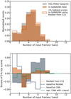 |
Fig. A.2 Same as Fig. A.1 for r-band. |
| In the text | |
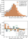 |
Fig. A.3 Same as Fig. A.1 for i-band. |
| In the text | |
Current usage metrics show cumulative count of Article Views (full-text article views including HTML views, PDF and ePub downloads, according to the available data) and Abstracts Views on Vision4Press platform.
Data correspond to usage on the plateform after 2015. The current usage metrics is available 48-96 hours after online publication and is updated daily on week days.
Initial download of the metrics may take a while.