| Issue |
A&A
Volume 697, May 2025
|
|
|---|---|---|
| Article Number | A24 | |
| Number of page(s) | 21 | |
| Section | Extragalactic astronomy | |
| DOI | https://doi.org/10.1051/0004-6361/202451615 | |
| Published online | 30 April 2025 | |
The dust polarisation and magnetic field structure in the centre of NGC253 with ALMA
1
DIFA, Università di Bologna, via Gobetti 93/2, I-40129 Bologna, Italy
2
INAF, Istituto di Radioastronomia, Via Gobetti 101, I-40129 Bologna, Italy
3
IRAP, Université de Toulouse, CNRS, CNES, UPS, (Toulouse), France
4
Department of Physics, School of Sciences and Humanities, Nazarbayev University, Astana 010000, Kazakhstan
5
LERMA, Observatoire de Paris, PSL Research University, CNRS, Sorbonne Universités, 75014 Paris, France
6
Kavli Institute for Particle Astrophysics & Cosmology (KIPAC), Stanford University, Stanford, CA 94305, USA
7
Department of Physics & Astronomy, University of South Carolina, Columbia, SC 29208, USA
8
Center for Interdisciplinary Exploration and Research in Astrophysics (CIERA) Northwestern University, Evanston, IL 60208, USA
9
Department of Astronomy, University of Maryland, College Park, MD 20742, USA
⋆ Corresponding author.
Received:
22
July
2024
Accepted:
7
March
2025
Abstract
Context. Magnetic fields (B fields) have an impact on galaxy evolution on multiple scales. They are particularly important for starburst galaxies, where they play a crucial role in shaping the interstellar medium (ISM), influencing star formation processes and interacting with galactic outflows.
Aims. The primary aim of this study is to obtain a parsec-scale map of the dust polarisation and B field structure within the central starburst region of NGC253. This includes examining the relationship between the morphology of B fields, galactic outflows, and the spatial distribution of super starclusters (SSCs), to understand their combined effects on the galaxy’s star formation and ISM.
Methods. We used ALMA full polarisation data in Bands 4 (∼145 GHz) and 7 (∼345 GHz) with a resolution of ∼25 and ∼5 pc scale, respectively. The Stokes I, Q, and U maps of the two bands have been used to compute the polarised intensity (PI), polarisation fraction (PF), B field orientation on the plane of the sky, and dispersion angle function (𝒮) maps. We computed the pixel-by-pixel uncertainties of these maps taking into account the covariance between the Stokes parameters I, Q, and U. The uncertainty allowed us to detect values of PF as low as ∼0.1% with a S/N (signal-to-noise ratio) greater than 3. Through a spectral energy distribution (SED)-fitting analysis including archival data, we investigated the main emitting components that contribute to the total and polarised emission in several areas of the starburst region.
Results. According to our SED-fitting analysis, the observed Band 4 emission is a combination of dust, synchrotron, and free-free components, while Band 7 traces only dust. The PF of the synchrotron component measures ∼2%, while that of the dust component is ∼0.3%. The B field orientation maps in both bands at a common resolution show that the same B field structure is traced by dust and synchrotron emission at scales ∼25 pc. The B field morphology suggests a coupling with the multiphase outflow, while the distribution of PF in Band 7 shows to be correlated with the presence of SSCs. We observed a significant anti-correlation between PF and column density in both Bands 4 and 7. A negative correlation between PF and 𝒮 was observed in Band 4 but was nearly absent in Band 7 at a native resolution, suggesting that the tangling of B field geometry along the plane of the sky is the main cause of depolarisation at ∼25 pc scales, while other factors play a role at ∼5 pc scales.
Key words: techniques: interferometric / techniques: polarimetric / galaxies: ISM / galaxies: magnetic fields / galaxies: starburst / galaxies: star clusters: general
© The Authors 2025
 Open Access article, published by EDP Sciences, under the terms of the Creative Commons Attribution License (https://creativecommons.org/licenses/by/4.0), which permits unrestricted use, distribution, and reproduction in any medium, provided the original work is properly cited.
This article is published in open access under the Subscribe to Open model. This email address is being protected from spambots. You need JavaScript enabled to view it. to support open access publication.
1. Introduction
Decades of observational and theoretical research have confirmed the ubiquitous existence of magnetic fields (B fields) in external galaxies (Lopez-Rodriguez et al. 2022b; Shukurov & Subramanian 2021; Beck et al. 2019; Krause 2019; Basu & Roy 2013; Moss et al. 2012). From a theoretical point of view, these fields significantly influence various astrophysical processes and thus affect the evolution of galaxies at multiple scales. Their effects include driving mass inflows of gas into the centres of galaxies (Kim & Stone 2012), and controlling the collapse of molecular clouds, which is critical for star formation (Hennebelle & Inutsuka 2019). Observations have also established a close correlation between B fields and the properties of the interstellar medium (ISM) in their host galaxies. Studies have indicated links between the strength of B fields and the star formation rate (SFR) in galaxies (Beck et al. 2019), the pitch angle of B fields and the molecular gas in spiral arms (Van Eck et al. 2015), the strength of large-scale ordered B fields and the rotational velocity of galaxies (Tabatabaei et al. 2013), as well as the strength of B fields and both gas density and SFR density (Chyży et al. 2017).
Spiral galaxies have large-scale ordered magnetic fields, with an average strength of about 5 ± 2 μG, while the total magnetic field strength (which includes both the ordered and perturbed component) is around 17 ± 14 μG (Beck et al. 2019). In face-on spiral galaxies, the magnetic field generally shows a kiloparsec-scale spiral pattern, with polarised emissions mainly aligned with interarm regions and peaking at the inner edges of spiral arms. This is due to a higher level of turbulence within the arms compared to interarm regions (Fletcher et al. 2011; Beck 2015). In edge-on spiral galaxies, the magnetic field exhibits a dual morphology: one component parallel to the disk’s midplane and another forming an X-shaped structure extending several kiloparsecs above and below the disk (Krause et al. 2020). The exact origin of the X-shaped magnetic fields in these halos remains unknown.
B fields are especially important for starburst galaxies. The strongest B fields (50–300 μG) have been observed in the core of the starburst sources (Lopez-Rodriguez 2023; Lopez-Rodriguez et al. 2021; Thompson et al. 2006). The energy densities derived from synchrotron radiation suggest that magnetic energy can exceed thermal and kinetic energies, implying that magnetic fields are essential to the dynamics and evolution of these starburst sources (Heesen et al. 2011). Far-infrared (FIR) polarimetric observations indicated an equipartition between turbulent magnetic and turbulent kinetic energy in the central ∼1 kpc galactic outflows (Lopez-Rodriguez 2023; Lopez-Rodriguez et al. 2021). The large scale B field structures in starburst systems have been observed to be aligned with the outflow activity (Heesen et al. 2011; Lopez-Rodriguez et al. 2021). This may have an effect on the galaxy’s subsequent evolution, since the outflow can drag material from the galaxy disk out into the circumgalactic medium (CGM) (Lopez-Rodriguez et al. 2021; Lopez-Rodriguez 2023), thereby enriching it (Martin-Alvarez et al. 2021). Analyses of simulations and observations of starburst systems have further suggested that B fields play an important role in the post-starburst phase, and are potentially responsible for the quenching of star formation activity by preventing the collapse of giant molecular clouds (Pattle et al. 2023; Tabatabaei et al. 2013).
Most of our knowledge of B fields in external galaxies comes from radio polarimetric observations in the 3 − 20 cm wavelength range (Stein et al. 2019; Beck 2015). At these wavelengths, the emission is dominated by synchrotron radiation arising mostly in the warm and diffuse phase of the ISM of galaxies (Beck & Wielebinski 2013). Observations of polarised light at FIR and sub-millimetre wavelengths offer an alternative probe of the magnetic field structure in colder and denser environments. In the presence of magnetic fields, the major axis of the elongated dust grains tends to align perpendicular to the B field. The physical process leading to alignment remains debated; proposed mechanisms include paramagnetic alignment (Davis & Greenstein 1951) and radiative torques (e.g. Hoang & Lazarian 2014). The thermal emission from dust in the FIR and millimetre wavelength range is thus linearly polarised, with the E-vector pointing perpendicular to the field. The measured polarisation angle (PA) rotated by 90° traces the B field orientation, projected in the plane of the sky.
Efforts to map the dust polarisation in external galaxies have significantly increased over the past decade, largely thanks to the improved resolution and sensitivity provided by the High-Angular Wideband Camera Plus (HAWC+; Harper et al. 2018; Dowell et al. 2010) onboard the Stratospheric Observatory For Infrared Astronomy (SOFIA). With HAWC+, the Survey on extragALactic magnetiSm with SOFIA (SALSA) Legacy Program (SALSA; Lopez-Rodriguez et al. 2022a) mapped the polarised dust emission from fourteen nearby galaxies (d < 20 Mpc, including NGC253) at 0.1−1 kpc scales in the 53 to 214 μm wavelength range. The first results from SALSA indicate typical polarisation fractions of 3% in galaxy disks, with starburst galaxies tending to exhibit lower polarisation fractions than normal spiral galaxies. The B field orientations inferred from the SALSA observations tend to be less ordered than the results obtained from polarised synchrotron emission at GHz frequencies (Surgent et al. 2023), suggesting that the magnetic field structure in the cold gas traced by dust polarisation may be more dominated by morphological complexity due to star formation activity and kinematic turbulence than the warmer, diffuse ISM (Borlaff et al. 2023). For the three starburst galaxies in the SALSA sample, the dust polarisation measurements indicated extraplanar B field structures perpendicular to the galaxy disk, physically associated with outflowing material in those systems (Lopez-Rodriguez et al. 2021; Lopez-Rodriguez 2023).
In this paper, we analyse polarisation observations made with the Atacama Large Millimeter Array (ALMA) Bands 4 (∼145 GHz) and 7 (∼345 GHz) across the central ∼200 pc of the nearby starburst galaxy NGC253. The primary aims of this study are to obtain a parsec-scale map of the dust polarisation and B field structure within the dense star-forming gas, and identify whether there is evidence for a physical connection between the observed magnetic field structure and dust polarisation properties and the starburst activity and/or outflow. The paper is organised as follows: we present our target and describe the ALMA observations in Sect. 2. In this Section, we describe the polarisation calibration and imaging procedures, including the method that we used to characterise the noise and hence estimate the uncertainties on the polarisation quantities that we infer. We discuss our ALMA maps of polarised intensity, polarisation fraction and B field orientations in Sect. 3, including a comparison of the polarisation properties at matched resolution. We also quantify the dispersion in the polarisation angles at the two bands. In order to interpret the polarisation results at the two ALMA bands, we performed a region-based total intensity spectral energy distribution (SED)-fitting analysis to estimate the relative contributions of dust, synchrotron and free-free emission at Band 4; this analysis is presented in Sect. 4. In Sect. 5, we discuss the observed magnetic field structure in relation to other ISM and star formation components of NGC253, the relative contributions of dust and synchrotron emission, and compare our results for the polarisation fraction and polarisation angle dispersion to Planck results for our Galaxy. We summarise our main conclusions in Sect. 6. In Appendix A we show the images of polarisation fraction and B field orientations. In Appendix B we present a table listing the results of the SED-fitting analysis. A table listing the archival data that we used for our analysis is presented, with the corresponding project codes, in Appendix C.
2. Data
2.1. Target: NGC253
NGC253 is a nearby, highly inclined, tilted, starburst galaxy (distance D = 3.5 Mpc, inclination i ∼ 78°, position angle of the long axis θ ∼ 52°; Rekola et al. 2005; Pence 1980; Lucero et al. 2015). As the nearest system hosting an exceptional multiphase galactic wind, it has been extensively studied in many wavebands, including X-ray (Strickland et al. 2000), optical (Watson et al. 1996), infrared (Sugai et al. 2003), sub-millimetre (Bolatto et al. 2013a), and GHz radio, including polarisation (Turner & Ho 1985; Heesen et al. 2009, 2011). The central starburst activity in NGC253 is fuelled by gas accretion along the bar (Paglione et al. 2004), resulting in a SFR of ≈ 2 M⊙ yr−1 (Bendo et al. 2015; Leroy et al. 2015; Ott et al. 2005) across the central few hundred parsecs. This intense star formation drives a massive outflow (Walter et al. 2017). In this region signs of shock activities have also been found (Humire et al. 2025). The mass outflow rate has been estimated to be 14−39 M⊙ yr−1 in the cool molecular phase (Krieger et al. 2019) and approximately 2.8 M⊙ yr−1 for the north-western side and around 3.2 M⊙ yr−1 for the south-eastern side in the warm ionised phase (Lopez et al. 2023). Recently, the molecular gas content of NGC253’s outflow and the nascent superstar clusters (SSCs) that account for a large fraction of the star formation activity in the nuclear starburst have been studied in detail with ALMA (e.g. Bolatto et al. 2013a; Leroy et al. 2015, 2018; Zschaechner et al. 2018; Krieger et al. 2019; Levy et al. 2021, 2022; Mills et al. 2021). These studies have shown that the outflowing molecular gas is located mostly around the edge of the wind. The most prominent outflow structure in ALMA molecular emission line maps is the south-western streamer, from which ∼350 GHz dust continuum emission has also been detected. Estimates of the molecular mass outflow rate range between ∼ 3 − 9 M⊙ yr−1 (Bolatto et al. 2013a) and ∼ 25 − 50 M⊙ yr−1 (Zschaechner et al. 2018), that is, a mass-loading factor of ∼5. The SSCs in the centre of NGC253 are young ∼0.01 − 3 Myr, with typical stellar masses of 104 − 106 M⊙ and a full width at half maximum (FWHM) sizes of 0.4 − 0.7 pc. As projected on the sky, the SSCs appear to be aligned along a thin linear structure with length ∼150 pc. Modelling of the SSCs’ morphology and kinematics suggests that they are distributed on an elliptical ring with a semimajor (semiminor) axis of 110 (60) pc, which we observe edge-on (Levy et al. 2022).
At far-infrared to radio wavelengths, NGC253’s integrated SED is well-described by a combination of synchrotron, free-free and thermal dust emission, with a very steep synchrotron spectrum at high radio frequencies (Peel et al. 2011). Thermal dust emission seems to dominate the global SED at the frequencies of ALMA Band 4 (145 GHz) and Band 7 (343.5 GHz). As one of the nearest galaxies with an extremely bright dust continuum (7.4 Jy at 353 GHz, Planck Collaboration VII 2011), NGC253 is an ideal target for extragalactic dust polarisation studies. SOFIA/HAWC+ observations by SALSA at 89 and 154 μm indicate that on ∼100 pc spatial scales, the thermal dust emission is ∼1% polarised in the central region, with higher polarisation fractions further out in the disk. The orientation of the B field inferred from the SALSA measurements suggests that the magnetic field traced by dust (Lopez-Rodriguez & Tram 2024) is preferentially aligned with the galactic disk, except in the central region where the field also shows perpendicular structure (Lopez-Rodriguez 2023; Lopez-Rodriguez et al. 2022a).
2.2. ALMA Band 4 and 7 observations
We obtained full polarisation observations of the central region of NGC253 with ALMA in Band 4 (Asayama et al. 2014) and Band 7 (Mahieu et al. 2012). The observations consisted of a single-pointing with a primary beam FWHM of ∼42 and ∼18″, respectively (see Fig. 1). The four cross-correlation visibilities (XX, XY, YX, YY) were recorded using the default frequency setup for continuum polarisation observations, time division mode (TDM), with four 2 GHz spectral windows, each divided into 64 channels. The central frequencies of the two bands are reported in Table 1. The observations were conducted with the C43-1 for Band 4 and C43-4 for Band 7, providing a nominal angular resolution of 1.7″ and 0.3″, and nominal maximum recoverable scale of ∼15″ and 3.8″, respectively.
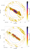 |
Fig. 1. Total intensity images. Band 4 (∼145 GHz) is shown on the top panel, Band 7 (∼345 GHz) on the bottom panel. The thick black contour corresponds to 3 × σI, while the grey thin contours correspond to [5, 7, 10, 30, 100]×σI. The concentric circles overlaid on the images are the annular regions used for the noise analysis (see Sect. 2.5). The thick and dotted blue circles correspond to 1/3 of the HPBW and the full HPBW of the image, respectively. The red circles have as radii multiples of n * 1/3 of the HPBW, where n ranges from 2 to 5. |
The observations were executed using the session observing scheme, which is standard for polarisation projects with ALMA. Sessions consist of continuous execution of the same schedule until the required parallactic angle coverage for the polarisation calibrator has been achieved. A parallactic angle coverage of more than 60 degrees is needed to ensure a proper calibration of the instrumental polarisation (see following section). In general, this coverage is achieved with two to three executions of the schedule. Table 1 reports the details of the different sessions observed and the relevant properties derived in each session for the polarisation calibrator J0006-0623 that was used for both bands. This calibrator was observed at regular intervals in the standard phase calibrator – science target loop. The phase calibrator used for both bands was the quasar J0038-2459, while flux and bandpass calibrations were performed on quasar J2258-2758, or on J0006-0623. In Band 7, observations of an additional quasar J0046-2691 were included, providing an independent check on the calibration solutions.
Properties of the observing sessions.
2.3. Calibration
The data were calibrated using the CASA software package (version 5.6.1, CASA Team 2022) and the standard calibration scripts provided by the observatory. The current calibration scheme for polarisation projects is summarised in Nagai et al. (2016) and in the ALMA polarisation casaguide1. The total intensity calibration, deriving frequency and time dependent gains, is performed for each observing execution, while the polarisation calibration is done per session (combining consecutive executions). This calibration assumes that the polarisation calibrator has no circular polarisation (Stokes V = 0) and it derives the linear polarisation properties of the calibrator as well as the instrumental polarisation from the data, exploiting the parallactic angle variation. Table 1 reports the calibrator’s linear polarisation ratio, polarisation angle and parallactic angle range determined from the different sessions. We observed a 90° wrap of the parallactic angle range in our Band 4 observations. This is due to an intrinsic variation of the calibrator’s properties at all frequencies, as reported in the monitoring survey2.
The instrumental polarisation gains that we derived (Dterms < 4% for each antenna) were applied to all sources. To confirm the quality of the calibration, an image of the polarisation calibrator for each session was made. The Stokes I flux is normalised by the calibration procedure, so we measure a peak of ∼1 Jy/beam in both bands. The Stokes V images show no signs of residual instrumental polarisation. They have a root mean square (RMS) of 0.015 mJy/beam and 0.030 mJy/beam in Band 4 and Band 7, respectively.
2.4. Full-Stokes imaging
The calibrated sessions for each band were combined and imaged using the CASA task tclean. Continuum full Stokes (I, Q, U, V) images of the target and the calibrators were obtained in multi-frequency mode (mfs), using the clarkstokes deconvolver algorithm in which a Clark clean operates separately on each Stokes plane. A Briggs weighting scheme (Briggs 1995) with robust = 0.2 and 0.5 was used for imaging of Band 4 and 7 respectively. The resulting images in Band 4 have a synthesised beam of 1.54 × 1.33″ (26.1 × 22.1 pc), with a beam position angle bpa = 81.2 deg, and in Band 7 a beam of 0.32 × 0.28″ (5.4 × 4.8 pc), with a bpa = −88.5 deg. The RMS measured in Stokes I, Q and U, are reported in Table 2; these values are consistent with expectations from the radiometer formula. Stokes I images, shown in Fig. 1, are dynamic range limited in both Bands 4 and 7 with a signal-to-noise ratio (S/N) of 500 and 180, respectively.
Properties of the final images.
In order to compare the results at the two different frequencies, we convolved the data to a common resolution of 1.54 × 1.33″ (i.e. the Band 4 resolution). Additionally, the spectral energy distribution analysis presented in Sect. 4 required us to homogenise the data at all frequencies to the resolution of the archival VLA L-band data (2.2 × 2.2″, ∼37 pc). Table 2 reports the noise characteristics of the images at the different resolutions that we use in our analysis.
2.5. Noise characterisation
From the Stokes Q and U images, we constructed images of the linearly polarised intensity  , the polarisation fraction PF = PI/I, and the polarisation angle PA = 1/2arctan(U/Q). In polarisation studies, strong assumptions are often made about the noise properties of the measurements, such as neglecting the correlation between the total and polarised intensities and between the noise in Stokes Q and U images. Nevertheless, the covariance between the Stokes parameters can have a complex effect on the non-linear quantities derived, such as PF, PI, and PA, especially at low S/N (e.g., Montier et al. 2015). For this reason, we decided to compute the uncertainties taking into account the full covariance matrix of the Stokes I, Q, and U components. This is defined as
 (1)
(1)
where σXY is the covariance between the variables X and Y. We assume that circular polarisation (i.e. Stokes V) can be neglected. We compute the uncertainties on PF, PI, and PA taking into account the full covariance matrix. In this case, the noise in our derived quantities may be defined as follows:
 (2)
(2)
![Mathematical equation: $$ \begin{aligned} \sigma _{PI}^2&= \frac{1}{PI^2} ( Q^2 \sigma _{QQ} + U^2 \sigma _{UU} + 2QU\sigma _{QU} ) \, \, \, [(MJy/sr)^2] \end{aligned} $$](/articles/aa/full_html/2025/05/aa51615-24/aa51615-24-eq4.gif) (3)
(3)
![Mathematical equation: $$ \begin{aligned}\sigma _{PA}^2&= \frac{1}{4}\frac{Q^2 \sigma _{UU} + U^2 \sigma _{QQ} - 2QU\sigma _{QU}}{(Q^2 + U^2)^2} \, \, \, [rad^2]. \end{aligned} $$](/articles/aa/full_html/2025/05/aa51615-24/aa51615-24-eq5.gif) (4)
(4)
Readers can refer to Montier et al. (2015) and appendix B1 of Planck Collaboration Int. XIX (2015) for a full discussion on the impact of noise on estimates of PF, PI, and PA.
Since the ALMA data are provided with no per-pixel estimate of the noise correlation matrix, we estimate the noise correlation matrix elements of Equation (1) by computing covariances in signal-free regions of the I, Q, and U maps. We divided the images into five annuli of increasing radius (see Fig. 1). The central region is a circle with a radius equal to one-third of the Half Power Beam Width (HPBW) of the antenna primary beam. The subsequent concentric rings are determined by circles with radii ri = n × 1/3 × HPBW, with n ranging from 2 to 5. In each region, we computed the covariance matrix excluding the pixels with total intensity greater than 0.16 mJy/beam and 0.47 mJy/beam, corresponding to three times the RMS of the total intensity Band 4 and 7 images, respectively. The covariance matrix elements thus computed for each ring are listed in Table 3. The derived values are then employed to estimate the uncertainties in PF, PI, and PA for all pixels of that ring. These values are also used to debias the measured PF, following the modified asymptotic estimator formula proposed in Plaszczynski et al. (2014). The variances of the covariance matrix elements σQQ and σUU are roughly constant in the first three rings, as it is shown on Table 3. This would suggest the absence of large systematics outside the 1/3 of the HPBW.
Elements of the noise covariance matrix.
In order to facilitate a more direct comparison of the data in the two Bands, we converted the PI and total intensity estimates and relative uncertainties to MJy/sr. The scale factors of the conversion from Jy/beam to MJy/sr are 18 310 and 431 673 for Band 4 and 7, respectively.
2.6. Ancillary data
For the SED analysis presented in Sect. 4, we assembled archival data covering the frequency range from 1.4 GHz (λ ∼ 20 cm) to 690 GHz (λ ∼ 0.4 mm) taken with ALMA and the Very Large Array (VLA). The high frequency data are taken from the ALMA archive, and have resolutions ranging from ∼1 to 1.7″. The low frequency data are taken from VLA archive, and the image at the lowest frequency (1.4 GHz) has a resolution of 2.2″. The data at all frequencies were convolved to this resolution for the SED analysis. The original resolution of each image is reported in Table C.1, as well as the largest angular scale recovered, and the corresponding project code.
The images at 22 and 33 GHz used in the SED analysis in Sect. 4 were presented by Gorski et al. (2017, 2019). The resolutions of these datasets are 0.204″ × 0.121″ and 0.096″ × 0.045″, with maximum recoverable scales of 2.4″ and 1.6″ at 22 GHz and 33 GHz, respectively.
Finally, for the comparison of the magnetic field orientation with molecular gas distribution, we used archival ALMA observations of the CO(3-2) emission in NGC253. Of the available data, presented in Leroy et al. (2018), we selected those obtained with a compact configuration providing a resolution of 0.3 × 0.4 arcsec, very similar to that of our full polarisation data in Band 7.
3. ALMA polarisation images
Our final images of the polarised intensity and polarisation fraction at both ALMA bands at their native resolution are shown in the upper panels of Figs. 2 and A.1, respectively. The upper panels of Fig. A.2 show the orientation of the B field on the plane of the sky, computed by rotating the polarisation angle (PA) by 90°. For each polarisation quantity, we also show the corresponding S/N map, computed using the uncertainty σ defined in Sect. 2.5. In the lower panel of each Figure, red empty histograms indicate the distribution of pixels with S/N in total intensity above 3. The green and blue solid histograms represent the distribution of pixels after applying an additional threshold on the corresponding polarisation quantity of 1-sigma and 3-sigma, respectively.
3.1. Polarised intensity and polarisation fraction
Figure 2 shows the polarised intensity of the galaxy at Band 4 and Band 7, for all map pixels with a I/σI > 3. The white vectors represent the orientation of the magnetic field on the plane of the sky. For clarity, one vector is shown every two pixels (for Band 4 maps) and three pixels (for Band 7 maps).
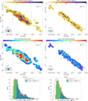 |
Fig. 2. Polarised intensity in the centre of NGC253. Upper panels: Maps of the linearly polarised intensity. The vectors indicate the magnetic field orientation and are displayed only at pixels where PI/σPI > 3. Centre panels: S/N maps of the polarised intensity with contours corresponding to [1, 3, 5, 10]×PI/σPI. White stars in the lower left panel indicate the positions of the SSCs catalogued by Leroy et al. (2018). The synthesised beam of the data is indicated in the bottom left corner, and the pixel selection threshold is shown in the top right corner. Both maps have been obtained selecting pixels with total intensity above 3σ. Bottom panels: Histograms of polarised intensity pixel values in the map. The empty histogram shows the distribution of pixels with total intensity above 3σ, while the solid green and blue histograms are the distribution of pixels with polarised intensity above 1σ and 3σ, respectively. The Band 4 and Band 7 results are shown in the top row and the bottom row, respectively. |
In Band 4, the median value of the polarised intensity is ≊0.96 MJy/sr with a standard deviation of ≊0.51 MJy/sr, measured over a region where I/σI > 3 and PI/σPI > 3. The PI map shows local maxima of PI ∼ 2.5 MJy/sr from four elongated bright spots situated to the north, south, east and west of the galaxy centre (from here after referred to as PIN, PIS, PIE and PIW). These maxima (identified in Fig. 7) do not have counterparts in total intensity.
The Band 7 observations access smaller physical scales within the starburst region. At this band, the polarised intensity distribution is more uniform, with a median of ≊ 40.28 MJy/sr and standard deviation of ≊ 13.22 MJy/sr (again considering only pixels with I/σI > 3 and PI/σPI > 3). The north and south elongated bright spots visible in Band 4 are resolved into several smaller local maxima with PI ∼ 50 MJy/sr. Particularly noteworthy are three of these maxima, two to the north and one to the south, which achieve values surpassing 80 Jy/sr. As for the Band 4 data, these local maxima do not clearly correspond to structures observed in total intensity.
Figure A.1 shows the PF maps measured in Band 4 and Band 7, superimposed with vectors that represent the orientation of the magnetic field. As in Fig. 2, signal-to-noise maps and histograms of the PF pixel values are also shown. The PF distribution measured in Band 4 with I/σI > 3 and PF/σPF > 3 has a median value of  % and standard deviation of ≊2.47%. Low PF values are concentrated in the innermost region (where the elongated bright spots in PI are located). This inner low PF area (with a median value of around 0.5%), coincides roughly with the region characterised by I/σI > 3 in Band 7.
The higher resolution of the Band 7 data allows us to study the distribution of PF in this region at spatial scales of ∼5 pc. The median computed with I/σI > 3 and PF/σPF > 3 is 1.06% with standard deviation of 0.90%. The map is not uniform, with several local minima apparently aligned along the galaxy midplane in the NE-SW direction.
In regions where I/σI > 3 and PF/σPF > 3 the minimum values of PF are 0.15% in Band 7 and 0.09% in Band 4. These values are comparable to the nominal ALMA minimum detectable degree of linear polarisation of 0.1%3.
3.2. Magnetic field orientation
In Fig. A.2, we show maps of the B field orientation as projected in the plane of the sky inferred from the Stokes Q and U of Band 4 and Band 7 images. The B field orientation is also shown as white vectors overlaid over the PI, and PF maps in Figs. 2, and A.1 in correspondence of pixels where PI/σPI > 3.
The B field structure probed by Band 4 observations is characterised by two main ordered components, one parallel to the mid-plane and one perpendicular to it. The two components meet in the central region of the galaxy, where the total intensity distribution observed in Band 4 peaks. A similar configuration has been seen in other edge-on galaxies at larger scales (∼0.1–1 kpc, Krause et al. 2020, 2006). The B field component parallel to the disk may be driven by the large-scale galactic B field, while the perpendicular component is likely driven by the galactic outflow pushed away by the starbursts activity.
The north and south maxima in the PI map align with areas where the magnetic field is perpendicular to the midplane. We discuss these regions in more detail in Sect. 4.
The orientation of the B field inferred from the Band 7 observations appears more chaotic than at Band 4. The histogram of inferred B field angles nonetheless indicates two main components that are parallel and perpendicular to the galactic midplane. This is evident in the red histogram (I/σI > 3) in the bottom right panel of Fig. A.2, where a prominent B field component with angle ∼50° can be seen, as well as a broader peak with angles ranging from −80° to −30°. This perpendicular component becomes a more obvious peak ∼ − 30° when we restrict our comparison to pixels with I/σI > 3 and PA/σPA > 3 (blue histogram in the right panel of Fig. A.2).
We note that the B field orientation that we infer in NGC253 differs from the Central Molecular Zone in our Galaxy. Both the Planck data at 850 GHz and the PILOT balloon-borne data at 240 μm (Mangilli et al. 2019) indicate a homogeneous magnetic field orientation that is tilted with respect to the Galactic plane by ≃22°. This difference could be explained by the different viewing angle or by the vastly different star formation efficiency which characterises the central regions of NGC253 and the Milky Way. Signs of a parallel and perpendicular B field component have been observed at 214 μm by the FIREPLACE survey (Butterfield et al. 2024; Paré et al. 2024).
3.3. Polarisation angle dispersion function
From our polarisation data, we also constructed a map of the polarisation angle dispersion function 𝒮, as defined in Kobulnicky et al. (1994) and Hildebrand et al. (2009). The angle dispersion function is computed as the median angular difference between a central pixel and the surrounding ones. The median is derived over an annulus of radius l (called ‘lag’) and width δl around the central pixel.
Regions where the magnetic field is well-ordered are characterised by 𝒮 ≊ 0°, while regions with irregular and disordered B fields will show progressively greater 𝒮 values. A fully random polarisation vector field will have 𝒮 ≊ 52° (Alina et al. 2016).
Maps of the polarisation angle dispersion function 𝒮 for our Band 4 and Band 7 ALMA maps are shown in Fig. 3. We chose to use a lag l and a width value corresponding to half the major axis of the clean beam of the ALMA maps (i.e. l = 0.15″ and δl = 0.15″ for Band 7 and l = 0.70″ and δl = 0.70″ for Band 4). We also computed the uncertainties of 𝒮 using Equation (9) from Planck Collaboration Int. XIX (2015).
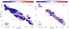 |
Fig. 3. Polarisation angle dispersion function in the centre of NGC253. Maps of the polarisation angle dispersion function obtained using the Band 4 (left) and Band 7 (right) data. Only pixels with I/σI > 3 in total intensity are shown. Vectors indicating the orientation of the B field vectors are overlaid only in correspondence of pixels where PI/σPI > 3. Yellow stars indicate the positions of the SSCs catalogued by Leroy et al. (2018). |
At Band 4, we identify three quasi-filamentary features with high values of 𝒮 (∼50°, red regions in Fig. 3), radiating out from the centre of the starburst region (referred to as SC in Sect. 4) where the perpendicular and parallel components of the polarisation vectors meet. These three regions of high values of 𝒮 (which we refer to as 𝒮-filaments) separate more extended areas where the polarisation angle directions are much more uniform (blue regions in Fig. 3).
At Band 7, the structure of 𝒮 is more complex, with an intricate web of 𝒮-filaments across the region with robust polarisation detections. Similarly to the 𝒮 distribution observed at Band 4, the 𝒮-filaments separate areas with distinct but homogeneous directions.
The complex network of 𝒮-filaments seen at Band 7 is only partially recovered at Band 4, primarily in the form of a long high 𝒮 region roughly parallel to the major axis. Due to the lower resolution, most of the structure observed in Band 7 is not discernible at Band 4.
3.4. Polarisation images at matched resolution
Measurements of polarisation properties strongly depend on resolution. To compare the results at different frequencies, we brought both images to the native resolution of the Band 4 data: 1.5″ × 1.3″. Figure 4 shows the resulting PF, 𝒮 and S/N of PF maps at both bands, overlaid with the B field orientation. The images have been masked to show only pixels characterised by I/σI > 3 in Band 7 at native resolution, while only B-filed vectors corresponding to regions where PI/σPI > 3 in both Band 4 and Band 7 are shown. The PF values of the smoothed Band 7 data have been debiased using the covariance matrix computed from the smoothed Stokes I, Q and U maps, following the same process described in Sect. 2.5. The resulting median and standard deviation values of I, PI, PF, B field orientation and 𝒮 maps are summarised in Table 4.
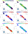 |
Fig. 4. Polarisation properties in the centre of NGC253 measured at the same resolution. Band 4 (left) and Band 7 (right) polarisation fraction (up), 𝒮 (centre) and S/N of PF (bottom) maps at the common resolution of 1.5 × 1.3″. In all panels, the inferred B field orientations are indicated with white vectors in correspondence of pixels where PI/σPI > 3 in Band 7. The images only show the central starburst region, inside the mask constructed from Band 7 data at its native resolution that includes pixels with I/σI > 3. |
Median and standard deviation values of key polarisation quantities.
Considering only pixels with I/σI > 3 and PF/σPF > 3, the PF distribution of the two images at common resolution is characterised by a median PF of 0.49 % for Band 4 and 0.39 % for Band 7. The overall PF configuration is similar in both bands when examined at the same resolution: the observed region appears more polarised at the edges of the mask, showing very low PF to the left and right of the galaxy’s centre.
The median values of 𝒮 measured at the same resolution are 27.15 degrees in Band 4 and 32.87 degrees in Band 7, indicating that there is still a slightly greater dispersion of the polarisation angles in Band 7. Overall, however, the 𝒮 maps at matched resolution are very similar, with local maxima situated in roughly the same regions of our observed field.
For the SED analysis, we smoothed the Band 4 and Band 7 images to 2.2 × 2.2″, corresponding to the resolution of the ancillary data described in Sect. 2.6. At this lower resolution, the median PF is 0.31% for Band 4 and 0.22% for Band 7. The decline in median PF with the increasing size of the observational beam is likely the result of beam depolarisation. This occurs when the polarisation and B field structures are smaller than the observational beam, such that the combination of their heterogeneous polarisation angles yields a net polarisation lower than the intrinsic value at smaller scales.
The distributions of polarisation fraction pixel values in the Band 4 and Band 7 maps at the two matched resolutions (1.5 × 1.3″ and 2.2 × 2.2″) are shown in Fig. 5. When smoothed to the same resolution, the PF distribution peaks at ∼0.3%−0.5% at both frequencies. The Band 4 distributions, however, show an extended tail of pixels with higher PF values. The pixels with high PF are mostly located in the SW edge of the regions where we have robust polarisation measurements (see Fig. 4). We discuss this feature further in Sect. 4.
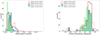 |
Fig. 5. Polarisation properties in the centre of NGC253 measured at the same resolution. Distributions of pixel values of the polarisation fraction (left panel) and B field orientation (right panel). Empty histograms represent the distributions of Band 4 pixels in the images at 1.5 × 1.3″ (pink) and at 2.2 × 2.2″ resolutions (red). The solid blue and green histograms represent the distributions at Band 7. Only pixels with S/N PF/σPF > 3 have been used for the computation of the histograms. |
The B field orientation inferred at both common resolutions is also very similar in the two bands. The histograms of the orientation of the B field (bottom panels of Fig. 5) peak strongly near ∼50°, indicating a component parallel to the galaxy midplane (characterised by a position angle of 52° ±1°, Lucero et al. 2015), with a weaker peak in both bands at ∼ − 60°, roughly orthogonal to the plane. From Fig. 4, it is evident that this perpendicular component is located in the same region at the two bands, corresponding to the local maximum of Band 4 total intensity.
The PF and B field distributions at the two bands at the same resolution do not show significant differences over most of the region that we analyse. The differences in the PF and B field distributions that are evident in Figs. A.1 and A.2 are lost when the images are convolved to a larger beam, meaning that Band 4 and Band 7 observations probe similar B field and polarisation structures at 1.3″ scales (∼25 pc).
4. SED-fitting analysis
The differences observed in the native resolution polarisation measurement at Band 4 and Band 7 are at least partially the result of the difference in resolution between the two bands. Nevertheless, the two bands may also trace different components of the ISM. The total intensity ratio between Band 4 and Band 7 in our spatially resolved data is higher than what we would expect from thermal dust emission. This indicates an additional emission component in Band 4. Previous analysis of the galaxy emission with multi frequency data also suggested a complex situation in terms of contribution of different emitting mechanisms. Peel et al. (2011) used data over the whole galaxy to determine a global spectral energy distribution (SED), which suggested the presence of free-free, dust and synchrotron emission across the 10 − 100 GHz range in the starburst region of the galaxy. Previous ALMA observations of the 99 GHz continuum and H40α emission with a spatial resolution of ∼30 pc in the central region indicated that free-free emission with an electron temperature Te = 3700 − 4500 K contributes ∼70% to the total flux at ν = 99 GHz (Bendo et al. 2015). In Humire et al. (2025) a detailed SED-fitting analysis spanning from near-UV to cm wavelengths was performed targeting at a resolution of ∼50 pc, revealing contributions of synchrotron, free-free and dust emission in the central molecular zone. Higher resolution observations at spatial scales of ∼5 pc showed a complex situation in which the relative contributions of dust, synchrotron and free-free vary spatially across the starburst region (Mills et al. 2021).
4.1. Estimating the Band 4 emission components
In order to estimate the relative contribution of the different emission mechanisms to the polarisation fraction observed in Band 4, we analysed the total intensity spectral energy distribution (SED) of the target, collecting archival data in the frequency range 1 − 300 GHz (see Table C.1 for details about the archival data used). All images were convolved to a 2.2″ round beam, corresponding to the largest beam of the available archival data, and regridded to have common pixelisation.
The SED-fitting was performed using the public code DustEMWrap (Compiègne et al. 2011)4. We constructed input SEDs using our full observed region, as well as a few regions with exceptional polarisation properties or intensities (see below for precise definitions). Our model fits describe the thermal dust emission using a Modified Black Body (MBB) and allow for contributions from synchrotron and free-free emission using the plugins provided in DustEMwrap. Since there are not noticeable signs of anomalous microwave emission (AME), we exclude any possible contribution from spinning dust. The absence of significant AME emission in NGC253 is also suggested in Mills et al. (2021) and Peel et al. (2011).
The mask used for the SED-fitting of the whole emission has been defined as the largest mask that includes pixels with I/σI > 3 in all archival images. This region is labelled SA in Fig. 7 and shown in pink contours. The variances used for the SED-fitting process are all assumed to be 0.4 × I2, where I is the total intensity of the corresponding data point.
Due to the degenerate contributions of the three processes in the frequency range 1 − 300 GHz, we fixed or restricted the range of several key physical parameters. The spectral index of the free-free emission was set to a fixed value of 0.118, a commonly observed value at sub-millimetre wavelengths (Condon 1992; Draine 2011). The temperature of dust emission was assumed to be Td = 30 K, a reasonable value for the centre of NGC253 (Melo et al. 2002; Weiß et al. 2008). For the synchrotron spectral index αsyn we tested two extreme values: 0.45 and 0.75. These values cover the typical range observed in high-density starburst galaxies (Heesen et al. 2022). The intensities of the dust, synchrotron, and free-free emission and the emissivity index βd of the MBB were allowed to vary independently during the fit. Table B.1 reports the results of the SED-fitting, quoted as a range of values obtained when adopting the two extreme values of αsyn.
The decomposition obtained for the SED of the whole starburst region is shown in the upper left panel of Fig. 6. Both fits with αsyn = 0.45 and αsyn = 0.75 are shown. The model was able to fit the data with a reduced χred2 = 0.10 and 0.07, respectively. The βd values derived from SED-fitting across various regions align with those observed in other starburst galaxies (McKay et al. 2023).
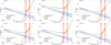 |
Fig. 6. SED-fitting analysis. The panels show the SED decomposition for the different regions (indicated in the top-left corner) discussed in Sect. 4. The observed measurements, shown by orange points with their uncertainties (±3σ) have been modelled using DustemWrap. The three fitted components: dust (in orange), synchrotron (in blue), and free-free (in green) are shown with shaded area indicating their range, assuming two different spectral index values. |
The SED-fitting results for the SA region indicate that the thermal dust emission contributes ≊90% of the Band 7 total intensity, while free-free and synchrotron contribute ≊8% and ≊1% respectively. In the spectral range 10 − 200 GHz, none of the three emission components is negligible. At Band 4, the contribution of dust, synchrotron and free-free emission to the total intensity is 22%−32%, 26%−14% and 51%−55%, respectively.
In order to estimate how the different contributions vary across the central starburst region, we repeated the analysis using a subset of pixels within different areas that are indicated in Fig. 7. These areas were selected by identifying pixels with elevated values of both total intensity and PI. Specifically, the SC area is defined by selecting the brightest 25% of pixels in the 2.2″ map of Band 4 total intensity. This area corresponds to the region where the parallel and perpendicular components of the magnetic field structure observed in Band 4 converge. The region SO is the complementary region of SC in SA. The areas labelled PIE, PIS, and PIW are identified by selecting the pixels with the highest 25% observed values of polarised intensity at Band 4. The subscripts E, S, and W denote the positions relative to the midplane of the galaxy. The SED decompositions for these regions are shown in the panels of Fig. 6. The names of the regions are indicated in the upper left corner of each panel. The SED-fitting results for these subregions are also listed in Table B.1. The overall trend observed in the SA area is roughly consistent across all other subregions, where Band 4 maps a similar contribution of free-free, synchrotron, and dust emissions, while Band 7 primarily traces dust.
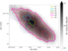 |
Fig. 7. Regions used for the SED-fitting analysis. Band 4 images of total (colour scale) and polarised (contours) intensity. The regions analysed in detail in Sect. 4 are indicated. |
4.2. Contributions to Band 4 polarisation
The above SED decomposition indicates that free-free emission, which is unpolarised (Rybicki & Lightman 1986), dominates the total Band 4 intensity. Our polarisation fraction measurements at Band 4 are thus due to a combination of synchrotron and dust emission, both polarised, diluted by the unpolarised free-free emission. However, we can use our SED decomposition results to estimate the polarisation fractions of the dust and synchrotron emission independently. We assume that only synchrotron and thermal dust contribute to the polarised emission in both ALMA bands. The polarisation fraction of the synchrotron emission is not expected to strongly vary across the frequency range of our data (see Sokoloff et al. 1998), and we assume that it is constant. Not much is known about possible frequency variations of the thermal dust polarisation fraction. The analysis of the all sky Planck data detected no systematic trend over the range 100–353 GHz, albeit with large uncertainties. Combining this result with very limited observations of specific sky regions in the FIR has led models (e.g., Hensley & Draine 2021) to assume no spectral variations of the dust polarisation fraction as long as dust particles are large enough to align with the magnetic field. Here we also follow this assumption and assume no frequency variations of the thermal dust polarisation fraction over the range observed with ALMA. Under these assumptions, the observed polarised intensities in Bands 4 and 7 can be written simply as
 (5)
(5)
where Isyn and Idust are the total intensity of the synchrotron and thermal dust emission, PFsyn and PFdust are the polarisation fraction of the synchrotron and dust emission (constant in Band 4 and 7 due to the assumptions we made), and the subscripts B4 and B7 refer to ALMA measurements in Bands 4 and 7, respectively.
The polarisation fractions can be deduced by inverting Equation (5), leading to
 (6)
(6)
 (7)
(7)
We measured PIB4 and PIB7 from the PI maps in Band 4 and Band 7, and derived the PFdust and PFsyn using the SED-fitting results for Isyn, Iff and Idust for the two bands. Inside the SA mask (pink contour in Fig. 7), the estimated polarisation fraction for the synchrotron component ranges from PFsyn = 1.78 − 3.44% (depending on the adopted synchrotron spectral index) and the dust polarisation ranges from PFdust = 0.25 − 0.27%. The measured polarisation fraction, which includes contributions from both dust and synchrotron components, is PFmeas.,B4 = 0.55% at Band 4 and PFmeas.,B7 = 0.31% at Band 7.
For all regions where we conducted the SED-fitting, the synchroton and dust polarisation fractions obtained using the above approach are listed in the last two columns of Table B.1. The reduced χ2 of the SED-fittings are also reported.
5. Discussion
5.1. Variations in the polarisation fraction
The measured polarisation fraction in Band 4 is ∼0.50%−0.70% across the starburst area, dropping to ∼0.17% in the SC region. From our SED-fitting analysis, this corresponds to PFdust of 0.25% for SA and 0.08% for SC. A decrease in the measured PF in sub-mm data is usually attributed to a gradual loss of alignment of dust grains, fluctuations in the orientation of the B field along the line-of-sight (LOS), or tangling of the B fields on scales smaller than the observational resolution, causing depolarisation (Planck Collaboration Int. XIX 2015). In addition to these effects, the observed decrease of PF in Band 4 can also be attributed to a contamination of non-polarised free-free emission, as our SED-fitting suggests. Interestingly, the decrease in polarisation fraction in the SC region is more pronounced for the dust component compared to the synchrotron component. The ratio between the polarisation fractions of the synchrotron and dust components,  , is 7–11 in the SO region, but it increases to 11–27 in the SC region. The regions PIE, PIS and PIW are all characterised by a relatively strong synchrotron component of PF. The region PIS and PIW are also characterised by a large
  ratio (around 10–18). This may be linked to the presence of the extended multi-phase outflow (see Sect. 5.2).
We can summarise the SED-fitting results as follows:
-
The different polarisation fractions observed at Band 4 and 7, after being smoothed to the same resolution, can be attributed to the distinct contributions of synchrotron, dust and free-free to the total emission, combined with the different characteristic polarisation fraction of the dust and synchrotron components at these frequencies. At Band 7, the total intensity is dominated by dust, while at Band 4 the emission is mostly due to free-free, with non-negligible, roughly equivalent contributions from dust and synchrotron. The high polarisation fraction of the synchrotron component is likely the main factor behind the higher observed polarisation fraction in Band 4.
-
In all the regions, the polarisation fraction of the synchrotron component is higher than that of the dust component. In particular, The ratio between the polarisation fractions of the synchrotron and dust components,
 , is 7.2–12.7 in the region SA, 11.0–26.8 in the SC, 6.6–11.3 in SO, 5.7–11.0 in PIE, 10.5-17.7 in PIS and 8.5-16.1 in PIW.
 -
The estimated PFdust and measured PF in Band 7 exhibit comparable values. Given the assumption of constant polarisation fraction of both the synchrotron and dust components over the frequency range 100 − 353 GHz, we can deduce that in Band 7 the polarisation fraction is due almost entirely to dust with negligible effect due to synchrotron.
-
The inferred magnetic field structure (shown in Fig. 4) is common to both bands, and thus appears relatively insensitive to the different emission processes that dominate the polarisation in the two bands.
-
The depolarisation within the central region (SC) appears to be more pronounced for the dust component than for the synchrotron component. This suggests that the degradation of the alignment of dust grains, contributing to PFdust, may play a role in the observed depolarisation. Multiple phenomena could explain the dust depolarisation in this region, including a differential tangling of the B field between dense and more diffuse part of the LOS.
5.2. The B field morphology and outflow in the centre of NGC253
The nuclear starburst of the galaxy NGC253 is responsible for launching a large multiphase outflow which extends to several kpc. This structure is detected across the electromagnetic spectrum, including X-ray (Strickland et al. 2000; Lopez et al. 2023), ionised gas (Westmoquette et al. 2011), molecular gas (Bolatto et al. 2013a; Krieger et al. 2019) and radio (Heesen et al. 2011).
The morphological structure of the outflow varies significantly depending on the observational wavelength. Optical observations (particularly Hα) and X-ray observations reveal a prominent biconical morphology that extends to several kpc in the SE and NW directions. From Hα kinematic modelling, the opening angle of the outflow is ∼60° (Westmoquette et al. 2011). Due to the orientation of the galaxy, the SE cone is more prominent and extended than the NW cone.
The molecular phase of the outflow, traced by CO(1-0) and CO(3-2) emission lines, is characterised by a more concentrated structure situated along the edges of the biconical wind. One of the most prominent structures is a south-western (SW) streamer placed along the direction of the minor axis of the starburst region (see e.g. Bao et al. 2024). Enhancements in the CO emission, such as the SW streamer and other distinct features, might be due to individual clouds that are trapped, disrupted, and ejected in the outflow (Zschaechner et al. 2018).
Radio continuum emission indicates the presence of four prominent filaments (scale height of 150 ± 20 pc) surrounding the SE and NW cone (Heesen et al. 2011). In that study, the large scale B field structure was probed by radio polarisation observations at wavelengths of 6 cm and 3 cm, with resolutions of approximately 500 pc and 120 pc, respectively. The large scale B field lines inferred from the radio data slowly open away from the midplane of the galaxy, forming a characteristic X-shaped field centred on the nucleus. The total B field strength measured in the filaments is 46 ± 10 μG, with an ordered field strength of 21 ± 5 μG, which is high enough to counteract the pressure in the nuclear outflow (Heesen et al. 2011), suggesting a role of the B field in collimating the outflow.
Figure 8 shows a three-colour, multi-wavelength view of the central region of NGC253. The X-ray (blue colour), [NII] emission line (red) and CO(3-2) (green) emissions are shown in relation to the B field structure revealed by our Band 4 ALMA data. The white contours indicate the Stokes I emission in Band 4. The B field lines inferred from our Band 4 data are shown as white vectors. The vectors are displayed every two pixels and only where PI/σPI > 3. The cyan contour highlights the regions that show outflow components, identified using [NII] and Hα line integrated intensity from VLT/MUSE data (Cronin et al. in prep.). The SW streamer location, taken from Zschaechner et al. (2018), is indicated as a red arrow and labelled as SW. In Fig. 9, the upper panel shows the same three-colour image as Fig. 8 but zoomed in to provide a closer view of the central region, while the lower panel presents the RGB image superimposed with the Band 7 B field vectors. The white stars mark the position of the SSCs identified by Leroy et al. (2018) (see also Levy et al. 2021, 2022; Mills et al. 2021), which account for a large fraction of the star formation activity in the central starburst region. Three of these SSCs (labelled 4, 5 and 14 in Leroy et al. 2018) have been observed to show P-Cygni profiles in multiple lines, which suggest the presence of small outflow activities. Furthermore, some of these SSCs (4, 6, 10, 10NE, 11, 12, and 13) host H40α emission with exceptionally broad linewidths (δvFWHM ∼ 100 − 200 km s−1), suggesting that they contribute to driving the ionised component of the multi-phase outflow (Mills et al. 2021).
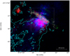 |
Fig. 8. Three-colour composite, multi-wavelength view of the central region in NGC253. Blue, red, and green show the X-ray emission from Lopez et al. (2023), optical [NII] data from Cronin et al. in prep., and CO(3-2) emission from Leroy et al. (2018), respectively. The B field lines and the emission of Stokes I flux of our ALMA Band 4 data are also shown as white vectors and yellow contours, respectively. The vectors are displayed every two pixels and only where PI/σPI > 3. The grey contours correspond to [5, 7, 10, 30, 100]×σI. The white rectangle marks the region shown on the upper panel of Fig. 9. |
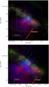 |
Fig. 9. Three-colour composite, multi-wavelength view of the central region in NGC253. Blue, red, and green show the X-ray emission from Lopez et al. 2023, optical [NII] data from Cronin et al. in prep., and CO(3-2) emission from Leroy et al. (2018), respectively. The B field lines and the emission of Stokes I emission of our ALMA Band 4 data (upper panel) and Band 7 data (lower panel) are also shown as white vectors and yellow contours, respectively. The vectors are displayed every two pixels and only where PI/σPI > 3. The grey contours correspond to [5, 7, 10, 30, 100]×σI. The red arrow marks the position of the molecular south-western streamer. The white rectangle on the upper panel marks the region shown on Fig. 8. The SSCs are marked as white stars and labelled following the notation of Leroy et al. (2018). The yellow contour mark the position of the SC region defined in Section 4. |
The base of the ionised component of the biconical outflow is a strong source of X-ray and [NII] emission. The B field inferred from our Band 4 data (Fig. 8 and upper panel of Fig. 9) seems to closely track the profile of the base of the outflow: the B-lines start to open away from the midplane at the peak position of the X-ray emission, assuming the same conical structure of the outflow. Away from the base of the outflow towards the SE, the B field lines seem to assume an ordered horizontal position relative to the midplane, until they are disrupted at the position of the SW molecular streamer. The same behaviour is observed on the northern side of the midplane, with the horizontal B-lines being disrupted towards a more vertical orientation along the direction of the SW streamer. The signal-to-noise ratio of our observations decreases away from the midplane. Consequently, it is not possible with our data to determine if the B field structure continues to follow the biconical outflow and align with the SW streamer’s direction.
Both the B field lines and the outflow cone are centred on the SC region defined in Sect. 4. This area is characterised by high molecular gas column density (as traced by the CO(3-2) map), and hosts four of the seven SSCs characterised by broad linewidth H40α emission. In the SC region, the SED-fitting analysis (see Sect. 4) also suggests a high synchrotron polarisation fraction indicating a coherent and ordered B field. A possible interpretation is that the high star formation rate drives the large scale winds which compress and order the B field, aligning it to the outflow cone. This interpretation is coherent with the picture of the SSCs characterised by broad linewidth H40α emission being the main driver of the large scale winds forming the biconical outflow.
The launch location of the wind seems to corresponds roughly to the SC region defined in Sect. 4, which is highlighted as yellow contour in both panels of Fig. 9. The highly tangled B field lines and the limited area for which we have robust Band 7 polarisation measurements complicate a more detailed comparison between the B field structure and the outflow morphology. From our data, it is not clear if the outflows due to SSCs 4, 5 and 14 in Levy et al. (2021) have a counterpart in the small scale B field morphology.
All the SSCs show a spatial relation with the measured PF in Band 7. This can be seen in the upper-right panel of Fig. A.1, where the positions of the SSCs are indicated by white stars. Locations with at least one SSC are characterised by local minima in PF measured in Band 7. Measuring the PF within one beam located on the SSCs, we get an average value below 0.4%, compared to a median PF value of 1.06% across the entire mask with I/σI > 3 and PF/σPF > 3. The correlation between local minima in PF and the position of SSCs is part of a more general relation that links the gas column density and polarisation fraction, which we discuss in the next subsection.
5.3. The PF vs NH relation
A trend for the thermal dust polarisation fraction to decrease with increasing gas column density was identified from the all-sky Planck data at 353 GHz (Planck Collaboration Int. XIX 2015), over a wide range of column densities from 1020 to 1023 H/cm2. This confirmed results from earlier ground-based observations of very bright regions that typically detected low polarisation fractions. Analysis of the Planck data revealed that the PF-NH anti-correlation extends to dense regions with no star formation. It is important to stress that since polarisation fraction measurements are positively biased upwards by noise and photon noise is always higher in low brightness regions, an anti-correlation can arise due to noise bias only. Therefore, only good quality de-biased polarisation data should be used to address this issue.
The physical origin for the anti-correlation between PF and NH is not completely clear. As dust alignment with the magnetic field could result from radiative alignment torques (RATs, e.g. Dolginov & Mitrofanov 1976; Andersson et al. 2015), the lack of photons in dark dense clouds could explain the observations. However, since polarisation sums as a spin-2 vector within the observational beam and along the LOS, the observed depolarisation could also result from the tangled structure of the magnetic field in dense regions. Additionally, since all models of dust alignment with the magnetic field predict a better alignment for large dust grains, the observed trend could also result from variations of the grain size distribution with column density. Explanations involving destruction of large dust grains (e.g. Lee et al. 2020; Hoang et al. 2021; Lopez-Rodriguez & Tram 2024) have been proposed for highly active star-forming regions.
Analysis of the all-sky Planck maps at 350 GHz did not reveal a systematic change in the relationships between the polarisation dispersion angle (see Sect. 3.3) and polarisation fraction with column density, indicating that tangling of the B field is the best explanation for the observed trend over the NH range sampled by the Planck data (Planck Collaboration Int. XIX 2015).
We used our debiased polarimetric observations and the archival ALMA observations of the CO(3-2) line (Leroy et al. 2018) to investigate the correlation between the polarisation fraction and the column density in NGC253. We calculated the column density NH from the CO(3-2) line fluxes using the relation NH2 = XCOICO(1 − 0), where XCO is the CO-to-H2 conversion factor for the CO(1-0) line integrated intensity ICO(1 − 0) (Bolatto et al. 2013b). We converted ICO(3 − 2) to ICO(1 − 0) using the empirical line ratio  . We adopted XCO = 0.5 · 1020[K km s−1 cm−2], a value consistent with other estimates for starburst galaxies (Bolatto et al. 2013b). Following Schinnerer & Leroy (2024) we assumed r31 = 0.31. We then estimated NH assuming NH ≊ 2N(H2).
Figure 10 shows the observed relation between PF and NH in our data computed at Band 4 (upper panel) and Band 7 (lower panel). The CO(3-2) data were convolved to the same resolution as the ALMA data, and only pixels with good S/N in CO(3-2) intensity (S/N > 3), Stokes I (S/N > 3) and PF (S/N > 3) are included.
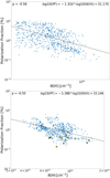 |
Fig. 10. Scatter plot of the observed polarisation fraction PF as a function of gas column density in NGC253. Band 4 data are shown on top panel, Band 7 in the bottom panel. The black line shows the trend derived from a fit to our data (see Eq. (8)). The yellow stars in the bottom panel indicate values computed at the location of the 14 SSCs (see Fig. 4). |
Our data show an anti-correlation between PF and NH given by:
 (8)
(8)
with a Pearson correlation coefficient ρ = −0.56 for Band 4, and by:
 (9)
(9)
with ρ = −0.50 for Band 7. The linear fit was done taking into account the uncertainties in PF using the orthogonal distance regression method. The trends in Fig. 10 indicate that the observed decrease of PF with NH in the Planck data continues at even higher column densities. A similar trend has been observed in Galactic cold cores and star-forming regions using JCMT and ALMA data (e.g., Koch et al. 2022; Lin et al. 2024), although it is often reported as a trend between polarisation fraction and total intensity rather than NH. We note that the values of PF observed in NGC253 across the column density range 1023 < NH < 4 × 1023 cm−2 tend to sit slightly higher than the trend line identified by Planck (Planck Collaboration Int. XIX 2015), although both our results and the Planck results show a large scatter. This discrepancy might be due to a more favourable orientation of the magnetic field direction in our observed field-of-view in NGC253.
5.4. PF versus 𝒮 relation
Recent polarisation studies also analyse the relation between PF and polarisation angle dispersion function 𝒮 (see Sect. 3.3), which quantifies the local order of PA, the magnetic field direction as projected on the sky (Alina et al. 2023; Planck Collaboration Int. XIX 2015). The all-sky maps of 𝒮 constructed from the Planck polarisation data at 350 GHz show intricate filamentary structures of high 𝒮 values that share no common structures with column density filaments, except possibly along the Galactic plane. These ridges appear to separate regions with rapidly varying polarisation angles from regions with more coherent PA. The Planck analysis showed a clear anticorrelation between PF and 𝒮, indicating that most of the variation in PF in the Planck data is depolarisation due to the tangling of the magnetic field within the beam and/or along the LOS.
In Planck Collaboration Int. XX (2015), predictions based on MHD simulations were compared to the data, showing a similar anti-correlation between PF and 𝒮, again suggesting that tangling of the field was responsible for the observed variations of PF. The simulations, however, were limited to column density values less than NH = 3 × 1022 cm−2, and the Planck data at the resolution used for polarisation analysis did not exceed NH = 1023 cm−2 where other physical effects could become important. The central starburst region of NGC253 allows us to explore a higher NH regime.
The upper and lower left panels of Fig. 11 show the correlation between PF and 𝒮 from our observations in Band 4 and Band 7. Only pixels with I/σI > 3, PF/σPF > 3 and 𝒮/σ𝒮 > 3 are included. Following Planck Collaboration Int. XIX (2015), we fit a straight line to the data in log-log given by
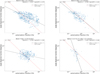 |
Fig. 11. Observed polarisation angle dispersion 𝒮 as a function of the polarisation fraction PF. Band 4 data are shown on the top left panel, Band 7 on the bottom left. On each plot, the black dashed line shows the trend derived from best fitting the data (see Equation (10)) excluding all pixels characterised by I/σI < 3, PF/σPF < 3 and 𝒮/σ𝒮 < 3, while the red line shows the best correlation obtained for the solar neighbourhood in the MW from the Planck data for reference. The upper right panel and the lower right panel shows the same plots computed in Band 4 and Band 7 smoothed at the common resolution of 1.5″ × 1.3″ using pixels belonging exclusively in the central starburst region, defined by the mask identified in Band 7 (at its native resolution) including pixels with S/N in total intensity larger than 3. On top of each panel the lag used to computed the angle dispersion function 𝒮 is indicated. |
 (10)
(10)
which we overlay on Fig. 11 in black. The linear fit was done taking into account the uncertainties in PF and 𝒮 using the orthogonal distance regression method. The correlation derived in the Planck Milky Way (MW) data is also shown on the figure as a red dotted line for reference. We find α = −0.427 and β = 1.374 for Band 4 data and α = −0.194 and β = 1.363 for Band 7 data. The Pearson correlation coefficients are ρ = −0.54 and ρ = −0.13 for Band 4 and Band 7, respectively, denoting an overall moderate anti-correlation for Band 4 and a little to no anti-correlation for Band 7.
The upper and lower right panels in Fig. 11 show the correlation between PF and 𝒮 for the two Band 4 and Band 7 images convolved to the Band 4 beam (1.5″ × 1.3″) and using a lag of 0.70″ for the 𝒮 computation. In this case, we applied the same mask used in Sect. 3.4, which only includes pixels with I/σI > 3 in Band 7 at native resolution. Additionally, we excluded all pixels with PF/σPF < 3 and 𝒮/σ𝒮 < 3. In this case, the anti-correlation is tight in both bands, with a Pearson index of −0.62 and −0.47 for Band 4 and Band 7, respectively. The anti-correlation observed at these scales at both bands is consistent with the similarities observed in maps of 𝒮 and PF, when smoothed to the same angular resolution (see Sect. 4). This indicates that the same magnetic field structure is traced by both dust and synchrotron emission in the central regions of NGC253 at ∼25 pc scales. Overall, the dependence of PF with 𝒮 and NH is quite similar to what was observed in Planck Collaboration Int. XIX (2015) in the MW.
In Band 7 at native resolution (lower left panel of Fig. 11), we see a different behaviour compared to the MW Planck results. At this scale (∼5 pc), the anticorrelation between NH and PF is still present, while we see no anticorrelation between 𝒮 and PF. This could indicate that thermal dust polarisation varies independently of the apparent B field tangling at column densities larger than NH ≃ 1023 cm−2 and scales ≲5 pc. It might suggest that, at scales of ∼5 pc in NGC253, the physical properties of the ISM, rather than the tangling of the B fields, control the observed depolarisation. Although we do not have access to ∼5 pc in Band 4 data, this divergent behaviour appears to be primarily caused by the different scales that characterise the Band 4 and Band 7 data, rather than the contributions of synchrotron and dust in these bands, since the correlation between PF and 𝒮 is recovered in Band 7 when the image is smoothed to the same resolution of Band 4, even though the slope and ρ index are different.
6. Conclusions
We have presented ALMA Band 4 (145 GHz) and Band 7 (350 GHz) polarisation measurements for the central ∼200 pc of the starburst galaxy NGC253. We have derived maps of the polarisation intensity and fraction, of the B field orientation and polarisation angle dispersion function, as well as the corresponding pixel-by-pixel signal-to-noise maps. The reported uncertainties on the polarisation results account for the covariance between the Stokes I, Q, and U parameters. The uncertainties allow us to detect PF as low as 0.1% with a S/N greater than 3. The polarisation properties measured at Bands 4 and 7 exhibit distinct characteristics, reflecting the different emission mechanisms that dominate at each band.
To evaluate the contributions of synchrotron, free-free, and dust in the region, we conducted an SED-fitting analysis using archival data from ALMA and VLA across the frequency range 1 − 350 GHz. At Band 7, the total intensity is mainly thermal dust emission, while Band 4 comprises significant contributions from free-free, dust, and synchrotron emission. By assuming a constant PF for the synchrotron and dust components in the 150 − 350 GHz range, we estimated the PF values for these components for our observed field and various smaller regions. We find that the synchrotron emission is more polarised than the dust emission in all analysed regions. This higher polarisation fraction of the synchrotron component appears to be the primary reason for the higher than expected polarisation observed in Band 4 maps, despite the significant contribution from (unpolarised) free-free emission at this frequency.
The analysis also revealed a sharp decline in PF estimates for the very centre of the starburst region (labelled as SC), which is characterised by high column density values and the presence of several super star clusters. This decline is likely caused by different factors, including significant non-polarised radiation from free-free emission and magnetic field fluctuations along the line-of-sight. The more pronounced decrease for the dust polarisation fraction in this central region suggests that differential tangling between the dense and more diffuse medium along the line of sight, and/or a dependence of the grain alignment or destruction of dust particles with environment may also play a role.
Using archival high-resolution ALMA observations of the CO(3-2) line and our debiased polarimetric data, we investigated the correlation between PF and NH in NGC253. We found a significant anti-correlation between PF and NH. This trend suggests that the decrease in PF with NH observed in Planck data (Planck Collaboration Int. XIX 2015) continues to even higher column densities.
Furthermore, the PF and the polarisation angle dispersion function 𝒮 are moderately anti-correlated in both bands when smoothed to spatial scales of ∼25 pc. At its native spatial resolution of ∼5 pc, we find no relationship between PF and 𝒮 in the Band 7 data. Our results suggest that the tangling of the B field is the main cause of the observed depolarisation at scales ∼25 pc, while other factors play a role at scales ∼5 pc. Further studies are required to test the effect of environment and spatial scale on the polarised emission of dust grains.
The similarity of the B fields orientation maps for Bands 4 and 7 images convolved at common resolution suggests that, on spatial scales ∼25 pc, the same magnetic field configuration is traced by both bands. This indicates that while the distinct contributions of synchrotron and dust influence the observed polarisation fraction characteristics, the magnetic field structures are largely unaffected at these scales.
From a qualitative analysis, the B field morphology seems to be coupled with the multi-phase outflow observed in the central region of NGC253. The B field probed by Band 4 data follows the base of the biconical outflow, mirroring its profile. The conical outflow and the B fields both seem to originate in the central region SC. This region is characterised by the presence of several super starclusters with exceptionally high broad linewidth H40α emission, which may be the main responsible in driving the ionised component of the multi-phase outflow. The high polarisation fraction of the synchrotron component estimated at the launch site of the outflow could be explained if the B fields are compressed and ordered by the strong winds produced by the SSCs. A coupling between the B field and the molecular outflow is seen mostly along the direction of the SW streamer, where the B field probed by Band 4 data seems to be disrupted on the northern sides of the midplane. Overall, our results highlight the interplay between magnetic fields, star formation, and outflows in shaping the central region of NGC253. A more quantitative analysis of the connection between the B field structure and outflow activity in NGC253 goes beyond the scope of this paper, and will be addressed in a future work.
Acknowledgments
This paper makes use of the following ALMA data: ADS/JAO.ALMA#2018.1.01358.S. ALMA is a partnership of ESO (representing its member states), NSF (USA) and NINS (Japan), together with NRC (Canada), NSTC and ASIAA (Taiwan), and KASI (Republic of Korea), in cooperation with the Republic of Chile. The Joint ALMA Observatory is operated by ESO, AUI/NRAO and NAOJ. DA acknowledges support from Nazarbayev University Faculty Development Competitive Research Grant No. 201223FD8821. ADB and SAC acknowledge partial support from grant NSF-AST 2108140.
References
- Alina, D., Montier, L., Ristorcelli, I., et al. 2016, A&A, 595, A57 [NASA ADS] [CrossRef] [EDP Sciences] [Google Scholar]
- Alina, D., Bernard, J. P., Yuen, K. H., et al. 2023, MNRAS, 518, 4466 [Google Scholar]
- Andersson, B. G., Lazarian, A., & Vaillancourt, J. E. 2015, ARA&A, 53, 501 [Google Scholar]
- Asayama, S., Takahashi, T., Kubo, K., et al. 2014, PASJ, 66, 57 [Google Scholar]
- Bao, M., Harada, N., Kohno, K., et al. 2024, A&A, 687, A43 [NASA ADS] [CrossRef] [EDP Sciences] [Google Scholar]
- Basu, A., & Roy, S. 2013, MNRAS, 433, 1675 [NASA ADS] [CrossRef] [Google Scholar]
- Beck, R. 2015, A&A Rev., 24, 4 [Google Scholar]
- Beck, R., & Wielebinski, R. 2013, Magnetic Fields in Galaxies (Dordrecht: Springer, Netherlands), 641 [Google Scholar]
- Beck, R., Chamandy, L., Elson, E., & Blackman, E. G. 2019, Galaxies, 8, 4 [NASA ADS] [CrossRef] [Google Scholar]
- Bendo, G. J., Beswick, R. J., D’Cruze, M. J., et al. 2015, MNRAS, 450, L80 [NASA ADS] [CrossRef] [Google Scholar]
- Bolatto, A. D., Warren, S. R., Leroy, A. K., et al. 2013a, Nature, 499, 450 [Google Scholar]
- Bolatto, A. D., Wolfire, M., & Leroy, A. K. 2013b, ARA&A, 51, 207 [CrossRef] [Google Scholar]
- Borlaff, A. S., Lopez-Rodriguez, E., Beck, R., et al. 2023, ApJ, 952, 4 [NASA ADS] [CrossRef] [Google Scholar]
- Briggs, D. S. 1995, Am. Astron. Soc. Meeting Abstr., 187, 112.02 [NASA ADS] [Google Scholar]
- Butterfield, N. O., Chuss, D. T., Guerra, J. A., et al. 2024, ApJ, 963, 130 [NASA ADS] [CrossRef] [Google Scholar]
- CASA Team (Bean, B., et al.) 2022, PASP, 134, 114501 [NASA ADS] [CrossRef] [Google Scholar]
- Chyży, K. T., Sridhar, S. S., & Jurusik, W. 2017, A&A, 603, A121 [NASA ADS] [CrossRef] [EDP Sciences] [Google Scholar]
- Compiègne, M., Verstraete, L., Jones, A., et al. 2011, A&A, 525, A103 [Google Scholar]
- Condon, J. J. 1992, ARA&A, 30, 575 [Google Scholar]
- Davis, L. Jr, & Greenstein, J. L. 1951, ApJ, 114, 206 [NASA ADS] [CrossRef] [Google Scholar]
- Dolginov, A. Z., & Mitrofanov, I. G. 1976, Ap&SS, 43, 291 [NASA ADS] [CrossRef] [Google Scholar]
- Dowell, C. D., Cook, B. T., Harper, D. A., et al. 2010, in Ground-based and Airborne Instrumentation for Astronomy III, eds. I. S. McLean, S. K. Ramsay, & H. Takami, SPIE Conf. Ser., 7735, 77356H [Google Scholar]
- Draine, B. T. 2011, Physics of the Interstellar and Intergalactic Medium (Princeton University Press) [Google Scholar]
- Fletcher, A., Beck, R., Shukurov, A., Berkhuijsen, E. M., & Horellou, C. 2011, MNRAS, 412, 2396 [CrossRef] [Google Scholar]
- Gorski, M., Ott, J., Rand, R., et al. 2017, ApJ, 842, 124 [CrossRef] [Google Scholar]
- Gorski, M. D., Ott, J., Rand, R., et al. 2019, MNRAS, 483, 5434 [NASA ADS] [CrossRef] [Google Scholar]
- Harper, D. A., Runyan, M. C., Dowell, C. D., et al. 2018, J. Astron. Instrum., 7, 1840008 [Google Scholar]
- Heesen, V., Krause, M., Beck, R., & Dettmar, R. J. 2009, A&A, 506, 1123 [NASA ADS] [CrossRef] [EDP Sciences] [Google Scholar]
- Heesen, V., Beck, R., Krause, M., & Dettmar, R. J. 2011, A&A, 535, A79 [NASA ADS] [CrossRef] [EDP Sciences] [Google Scholar]
- Heesen, V., Staffehl, M., Basu, A., et al. 2022, A&A, 664, A83 [NASA ADS] [CrossRef] [EDP Sciences] [Google Scholar]
- Hennebelle, P., & Inutsuka, S.-I. 2019, Front. Astron. Space Sci., 6, 5 [NASA ADS] [CrossRef] [Google Scholar]
- Hensley, B. S., & Draine, B. T. 2021, ApJ, 906, 73 [NASA ADS] [CrossRef] [Google Scholar]
- Hildebrand, R. H., Kirby, L., Dotson, J. L., Houde, M., & Vaillancourt, J. E. 2009, ApJ, 696, 567 [Google Scholar]
- Hoang, T., & Lazarian, A. 2014, MNRAS, 438, 680 [Google Scholar]
- Hoang, T., Tram, L. N., Lee, H., Diep, P. N., & Ngoc, N. B. 2021, ApJ, 908, 218 [NASA ADS] [CrossRef] [Google Scholar]
- Humire, P. K., Dey, S., Ronconi, T., et al. 2025, arXiv e-prints [arXiv:2501.15082] [Google Scholar]
- Kim, W.-T., & Stone, J. M. 2012, ApJ, 751, 124 [NASA ADS] [CrossRef] [Google Scholar]
- Kobulnicky, H. A., Molnar, L. A., & Jones, T. J. 1994, AJ, 107, 1433 [Google Scholar]
- Koch, P. M., Tang, Y.-W., Ho, P. T. P., et al. 2022, ApJ, 940, 89 [NASA ADS] [CrossRef] [Google Scholar]
- Krause, M. 2019, Galaxies, 7, 54 [NASA ADS] [CrossRef] [Google Scholar]
- Krause, M., Wielebinski, R., & Dumke, M. 2006, A&A, 448, 133 [NASA ADS] [CrossRef] [EDP Sciences] [Google Scholar]
- Krause, M., Irwin, J., Schmidt, P., et al. 2020, A&A, 639, A112 [NASA ADS] [CrossRef] [EDP Sciences] [Google Scholar]
- Krieger, N., Bolatto, A. D., Walter, F., et al. 2019, ApJ, 881, 43 [NASA ADS] [CrossRef] [Google Scholar]
- Lee, H., Hoang, T., Le, N., & Cho, J. 2020, ApJ, 896, 44 [Google Scholar]
- Leroy, A. K., Bolatto, A. D., Ostriker, E. C., et al. 2015, ApJ, 801, 25 [NASA ADS] [CrossRef] [Google Scholar]
- Leroy, A. K., Bolatto, A. D., Ostriker, E. C., et al. 2018, ApJ, 869, 126 [NASA ADS] [CrossRef] [Google Scholar]
- Levy, R. C., Bolatto, A. D., Leroy, A. K., et al. 2021, ApJ, 912, 4 [NASA ADS] [CrossRef] [Google Scholar]
- Levy, R. C., Bolatto, A. D., Leroy, A. K., et al. 2022, ApJ, 935, 19 [NASA ADS] [CrossRef] [Google Scholar]
- Lin, S.-J., Lai, S.-P., Pattle, K., et al. 2024, ApJ, 961, 117 [Google Scholar]
- Lopez, S., Lopez, L. A., Nguyen, D. D., et al. 2023, ApJ, 942, 108 [NASA ADS] [CrossRef] [Google Scholar]
- Lopez-Rodriguez, E. 2023, ApJ, 953, 113 [NASA ADS] [CrossRef] [Google Scholar]
- Lopez-Rodriguez, E., & Tram, L. N. 2024, ApJ, 975, 119 [Google Scholar]
- Lopez-Rodriguez, E., Guerra, J. A., Asgari-Targhi, M., & Schmelz, J. T. 2021, ApJ, 914, 24 [NASA ADS] [CrossRef] [Google Scholar]
- Lopez-Rodriguez, E., Clarke, M., Shenoy, S., et al. 2022a, ApJ, 936, 65 [Google Scholar]
- Lopez-Rodriguez, E., Mao, S. A., Beck, R., et al. 2022b, ApJ, 936, 92 [CrossRef] [Google Scholar]
- Lucero, D. M., Carignan, C., Elson, E. C., et al. 2015, MNRAS, 450, 3935 [NASA ADS] [CrossRef] [Google Scholar]
- Mahieu, S., Maier, D., Lazareff, B., et al. 2012, IEEE Trans. Terahertz Sci. Technol., 2, 29 [Google Scholar]
- Mangilli, A., Aumont, J., Bernard, J. P., et al. 2019, A&A, 630, A74 [NASA ADS] [CrossRef] [EDP Sciences] [Google Scholar]
- Martin-Alvarez, S., Katz, H., Sijacki, D., Devriendt, J., & Slyz, A. 2021, MNRAS, 504, 2517 [NASA ADS] [CrossRef] [Google Scholar]
- McKay, S. J., Barger, A. J., Cowie, L. L., Bauer, F. E., & Rosenthal, M. J. N. 2023, ApJ, 951, 48 [CrossRef] [Google Scholar]
- Melo, V. P., Pérez García, A. M., Acosta-Pulido, J. A., Muñoz-Tuñón, C., & Rodríguez Espinosa, J. M. 2002, ApJ, 574, 709 [NASA ADS] [CrossRef] [Google Scholar]
- Mills, E. A. C., Gorski, M., Emig, K. L., et al. 2021, ApJ, 919, 105 [NASA ADS] [CrossRef] [Google Scholar]
- Montier, L., Plaszczynski, S., Levrier, F., et al. 2015, A&A, 574, A135 [NASA ADS] [CrossRef] [EDP Sciences] [Google Scholar]
- Moss, D., Stepanov, R., Arshakian, T. G., et al. 2012, A&A, 537, A68 [NASA ADS] [CrossRef] [EDP Sciences] [Google Scholar]
- Nagai, H., Nakanishi, K., Paladino, R., et al. 2016, ApJ, 824, 132 [NASA ADS] [CrossRef] [Google Scholar]
- Ott, J., Weiss, A., Henkel, C., & Walter, F. 2005, ApJ, 629, 767 [NASA ADS] [CrossRef] [Google Scholar]
- Paglione, T. A. D., Yam, O., Tosaki, T., & Jackson, J. M. 2004, ApJ, 611, 835 [NASA ADS] [CrossRef] [Google Scholar]
- Paré, D., Butterfield, N. O., Chuss, D. T., et al. 2024, ApJ, 969, 150 [CrossRef] [Google Scholar]
- Pattle, K., Fissel, L., Tahani, M., Liu, T., & Ntormousi, E. 2023, in Protostars and Planets VII, eds. S. Inutsuka, Y. Aikawa, T. Muto, K. Tomida, & M. Tamura, ASP Conf. Ser., 534, 193 [Google Scholar]
- Peel, M. W., Dickinson, C., Davies, R. D., Clements, D. L., & Beswick, R. J. 2011, MNRAS, 416, L99 [NASA ADS] [CrossRef] [Google Scholar]
- Pence, W. D. 1980, ApJ, 239, 54 [NASA ADS] [CrossRef] [Google Scholar]
- Planck Collaboration VII. 2011, A&A, 536, A7 [NASA ADS] [CrossRef] [EDP Sciences] [Google Scholar]
- Planck Collaboration Int. XIX. 2015, A&A, 576, A104 [NASA ADS] [CrossRef] [EDP Sciences] [Google Scholar]
- Planck Collaboration Int. XX. 2015, A&A, 576, A105 [NASA ADS] [CrossRef] [EDP Sciences] [Google Scholar]
- Plaszczynski, S., Montier, L., Levrier, F., & Tristram, M. 2014, MNRAS, 439, 4048 [NASA ADS] [CrossRef] [Google Scholar]
- Rekola, R., Richer, M. G., McCall, M. L., et al. 2005, MNRAS, 361, 330 [NASA ADS] [CrossRef] [Google Scholar]
- Rybicki, G. B., & Lightman, A. P. 1986, Radiative Processes in Astrophysics (Wiley-VCH) [Google Scholar]
- Schinnerer, E., & Leroy, A. K. 2024, ARA&A, 62, 369 [NASA ADS] [CrossRef] [Google Scholar]
- Shukurov, A., & Subramanian, K. 2021, Astrophysical Magnetic Fields: From Galaxies to the Early, Cambridge AstrophysicsUniverse (Cambridge University Press) [Google Scholar]
- Sokoloff, D. D., Bykov, A. A., Shukurov, A., et al. 1998, MNRAS, 299, 189 [Google Scholar]
- Stein, Y., Dettmar, R. J., Weżgowiec, M., et al. 2019, A&A, 632, A13 [NASA ADS] [CrossRef] [EDP Sciences] [Google Scholar]
- Strickland, D. K., Heckman, T. M., Weaver, K. A., & Dahlem, M. 2000, AJ, 120, 2965 [NASA ADS] [CrossRef] [Google Scholar]
- Sugai, H., Davies, R. I., & Ward, M. J. 2003, ApJ, 584, L9 [Google Scholar]
- Surgent, W. J., Lopez-Rodriguez, E., & Clark, S. E. 2023, ApJ, 954, 53 [Google Scholar]
- Tabatabaei, F. S., Schinnerer, E., Murphy, E. J., et al. 2013, A&A, 552, A19 [NASA ADS] [CrossRef] [EDP Sciences] [Google Scholar]
- Thompson, T. A., Quataert, E., Waxman, E., Murray, N., & Martin, C. L. 2006, ApJ, 645, 186 [NASA ADS] [CrossRef] [Google Scholar]
- Turner, J. L., & Ho, P. T. P. 1985, ApJ, 299, L77 [NASA ADS] [CrossRef] [Google Scholar]
- Van Eck, C. L., Brown, J. C., Shukurov, A., & Fletcher, A. 2015, ApJ, 799, 35 [Google Scholar]
- Walter, F., Bolatto, A. D., Leroy, A. K., et al. 2017, ApJ, 835, 265 [NASA ADS] [CrossRef] [Google Scholar]
- Watson, A. M., Gallagher, J. S. I, Holtzman, J. A., et al. 1996, AJ, 112, 534 [NASA ADS] [CrossRef] [Google Scholar]
- Weiß, A., Kovács, A., Güsten, R., et al. 2008, A&A, 490, 77 [NASA ADS] [CrossRef] [EDP Sciences] [Google Scholar]
- Westmoquette, M. S., Smith, L. J., & Gallagher, J. S. I 2011, MNRAS, 414, 3719 [NASA ADS] [CrossRef] [Google Scholar]
- Zschaechner, L. K., Bolatto, A. D., Walter, F., et al. 2018, ApJ, 867, 111 [NASA ADS] [CrossRef] [Google Scholar]
Appendix A: Polarisation fraction and B field orientation images
Figure A.1 shows the PF maps measured in Band 4 and Band 7, superimposed with vectors that represent the orientation of the magnetic field. In Figure A.2, we show maps of the B field orientation as projected in the plane of the sky. The B field orientation is shown as white vectors overlaid in correspondence of pixels where PI/σPI > 3. Signal-to-noise maps and histograms of the B field orientation values are also shown at the bottom of both Figures.
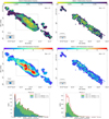 |
Fig. A.1. Polarisation fraction in the centre of NGC253. Upper panels: Maps of the polarisation fraction. The vectors indicate the magnetic field orientation and are displayed only at pixels where PI/σPI > 3. Centre panels: S/N maps of polarisation fraction with contours corresponding to [1, 3, 5, 10]×PF/σPF. White stars in the lower left panel indicate the positions of the SSCs catalogued by Leroy et al. 2018. Both maps have been obtained selecting pixels with total intensity above 3 sigma. Bottom panels: Histograms of the polarisation fraction pixel values in each map. The Band 4 and Band 7 results are shown in the left column and the right column, respectively. The plot annotations and pixel selection criteria are the same as in Figure 2. |
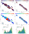 |
Fig. A.2. Magnetic field orientation in the centre of NGC253. Upper panels: Maps and corresponding vectors of the magnetic field orientation, obtained rotating the observed polarisation angle by 90 degrees. The vectors indicate the magnetic field orientation and are displayed only at pixels where PI/σPI > 3. Centre panels: S/N maps of the B field orientation with contours corresponding to [1, 3, 5, 10]×PA/σPA. White stars in the lower left panel indicate the positions of the SSCs catalogued by Leroy et al. 2018. Both maps have been obtained selecting pixels with total intensity above 3 sigma. Bottom panels: Histograms of the B field orientation pixel values in each map. Results from Band 4 and Band 7 observations are shown in the top row and the bottom row, respectively. The plot annotations and pixel selection criteria are the same as in Figure 2. |
Appendix B: SED-fitting results
Table B.1 illustrates the SED-fitting results obtained for the different areas shown in Figure 7. The SED decomposition for each region is shown in Figure 6. The SED-fitting analysis is explained in detail in Section 4.
SED-fitting results for the different regions analysed in Band 7 and Band 4.
Appendix C: ALMA and VLA archival images
For the SED analysis presented in Section 4, we assembled archival data covering the frequency range from 1.4 to 36 GHz taken with the Very Large Array (VLA)5 and from 100 to 690 GHz taken with ALMA6. The images have different resolutions reported in Table C.1, and have been convolved to the resolution of the lowest frequency (1.4 GHz) image (2.2″). The Table C.1 reports the details of the archival data.
Data used for the SED analysis in Section 4.
All Tables
All Figures
|
Fig. 1. Total intensity images. Band 4 (∼145 GHz) is shown on the top panel, Band 7 (∼345 GHz) on the bottom panel. The thick black contour corresponds to 3 × σI, while the grey thin contours correspond to [5, 7, 10, 30, 100]×σI. The concentric circles overlaid on the images are the annular regions used for the noise analysis (see Sect. 2.5). The thick and dotted blue circles correspond to 1/3 of the HPBW and the full HPBW of the image, respectively. The red circles have as radii multiples of n * 1/3 of the HPBW, where n ranges from 2 to 5. |
| In the text | |
|
Fig. 2. Polarised intensity in the centre of NGC253. Upper panels: Maps of the linearly polarised intensity. The vectors indicate the magnetic field orientation and are displayed only at pixels where PI/σPI > 3. Centre panels: S/N maps of the polarised intensity with contours corresponding to [1, 3, 5, 10]×PI/σPI. White stars in the lower left panel indicate the positions of the SSCs catalogued by Leroy et al. (2018). The synthesised beam of the data is indicated in the bottom left corner, and the pixel selection threshold is shown in the top right corner. Both maps have been obtained selecting pixels with total intensity above 3σ. Bottom panels: Histograms of polarised intensity pixel values in the map. The empty histogram shows the distribution of pixels with total intensity above 3σ, while the solid green and blue histograms are the distribution of pixels with polarised intensity above 1σ and 3σ, respectively. The Band 4 and Band 7 results are shown in the top row and the bottom row, respectively. |
| In the text | |
|
Fig. 3. Polarisation angle dispersion function in the centre of NGC253. Maps of the polarisation angle dispersion function obtained using the Band 4 (left) and Band 7 (right) data. Only pixels with I/σI > 3 in total intensity are shown. Vectors indicating the orientation of the B field vectors are overlaid only in correspondence of pixels where PI/σPI > 3. Yellow stars indicate the positions of the SSCs catalogued by Leroy et al. (2018). |
| In the text | |
|
Fig. 4. Polarisation properties in the centre of NGC253 measured at the same resolution. Band 4 (left) and Band 7 (right) polarisation fraction (up), 𝒮 (centre) and S/N of PF (bottom) maps at the common resolution of 1.5 × 1.3″. In all panels, the inferred B field orientations are indicated with white vectors in correspondence of pixels where PI/σPI > 3 in Band 7. The images only show the central starburst region, inside the mask constructed from Band 7 data at its native resolution that includes pixels with I/σI > 3. |
| In the text | |
|
Fig. 5. Polarisation properties in the centre of NGC253 measured at the same resolution. Distributions of pixel values of the polarisation fraction (left panel) and B field orientation (right panel). Empty histograms represent the distributions of Band 4 pixels in the images at 1.5 × 1.3″ (pink) and at 2.2 × 2.2″ resolutions (red). The solid blue and green histograms represent the distributions at Band 7. Only pixels with S/N PF/σPF > 3 have been used for the computation of the histograms. |
| In the text | |
|
Fig. 6. SED-fitting analysis. The panels show the SED decomposition for the different regions (indicated in the top-left corner) discussed in Sect. 4. The observed measurements, shown by orange points with their uncertainties (±3σ) have been modelled using DustemWrap. The three fitted components: dust (in orange), synchrotron (in blue), and free-free (in green) are shown with shaded area indicating their range, assuming two different spectral index values. |
| In the text | |
|
Fig. 7. Regions used for the SED-fitting analysis. Band 4 images of total (colour scale) and polarised (contours) intensity. The regions analysed in detail in Sect. 4 are indicated. |
| In the text | |
|
Fig. 8. Three-colour composite, multi-wavelength view of the central region in NGC253. Blue, red, and green show the X-ray emission from Lopez et al. (2023), optical [NII] data from Cronin et al. in prep., and CO(3-2) emission from Leroy et al. (2018), respectively. The B field lines and the emission of Stokes I flux of our ALMA Band 4 data are also shown as white vectors and yellow contours, respectively. The vectors are displayed every two pixels and only where PI/σPI > 3. The grey contours correspond to [5, 7, 10, 30, 100]×σI. The white rectangle marks the region shown on the upper panel of Fig. 9. |
| In the text | |
|
Fig. 9. Three-colour composite, multi-wavelength view of the central region in NGC253. Blue, red, and green show the X-ray emission from Lopez et al. 2023, optical [NII] data from Cronin et al. in prep., and CO(3-2) emission from Leroy et al. (2018), respectively. The B field lines and the emission of Stokes I emission of our ALMA Band 4 data (upper panel) and Band 7 data (lower panel) are also shown as white vectors and yellow contours, respectively. The vectors are displayed every two pixels and only where PI/σPI > 3. The grey contours correspond to [5, 7, 10, 30, 100]×σI. The red arrow marks the position of the molecular south-western streamer. The white rectangle on the upper panel marks the region shown on Fig. 8. The SSCs are marked as white stars and labelled following the notation of Leroy et al. (2018). The yellow contour mark the position of the SC region defined in Section 4. |
| In the text | |
|
Fig. 10. Scatter plot of the observed polarisation fraction PF as a function of gas column density in NGC253. Band 4 data are shown on top panel, Band 7 in the bottom panel. The black line shows the trend derived from a fit to our data (see Eq. (8)). The yellow stars in the bottom panel indicate values computed at the location of the 14 SSCs (see Fig. 4). |
| In the text | |
|
Fig. 11. Observed polarisation angle dispersion 𝒮 as a function of the polarisation fraction PF. Band 4 data are shown on the top left panel, Band 7 on the bottom left. On each plot, the black dashed line shows the trend derived from best fitting the data (see Equation (10)) excluding all pixels characterised by I/σI < 3, PF/σPF < 3 and 𝒮/σ𝒮 < 3, while the red line shows the best correlation obtained for the solar neighbourhood in the MW from the Planck data for reference. The upper right panel and the lower right panel shows the same plots computed in Band 4 and Band 7 smoothed at the common resolution of 1.5″ × 1.3″ using pixels belonging exclusively in the central starburst region, defined by the mask identified in Band 7 (at its native resolution) including pixels with S/N in total intensity larger than 3. On top of each panel the lag used to computed the angle dispersion function 𝒮 is indicated. |
| In the text | |
|
Fig. A.1. Polarisation fraction in the centre of NGC253. Upper panels: Maps of the polarisation fraction. The vectors indicate the magnetic field orientation and are displayed only at pixels where PI/σPI > 3. Centre panels: S/N maps of polarisation fraction with contours corresponding to [1, 3, 5, 10]×PF/σPF. White stars in the lower left panel indicate the positions of the SSCs catalogued by Leroy et al. 2018. Both maps have been obtained selecting pixels with total intensity above 3 sigma. Bottom panels: Histograms of the polarisation fraction pixel values in each map. The Band 4 and Band 7 results are shown in the left column and the right column, respectively. The plot annotations and pixel selection criteria are the same as in Figure 2. |
| In the text | |
|
Fig. A.2. Magnetic field orientation in the centre of NGC253. Upper panels: Maps and corresponding vectors of the magnetic field orientation, obtained rotating the observed polarisation angle by 90 degrees. The vectors indicate the magnetic field orientation and are displayed only at pixels where PI/σPI > 3. Centre panels: S/N maps of the B field orientation with contours corresponding to [1, 3, 5, 10]×PA/σPA. White stars in the lower left panel indicate the positions of the SSCs catalogued by Leroy et al. 2018. Both maps have been obtained selecting pixels with total intensity above 3 sigma. Bottom panels: Histograms of the B field orientation pixel values in each map. Results from Band 4 and Band 7 observations are shown in the top row and the bottom row, respectively. The plot annotations and pixel selection criteria are the same as in Figure 2. |
| In the text | |
Current usage metrics show cumulative count of Article Views (full-text article views including HTML views, PDF and ePub downloads, according to the available data) and Abstracts Views on Vision4Press platform.
Data correspond to usage on the plateform after 2015. The current usage metrics is available 48-96 hours after online publication and is updated daily on week days.
Initial download of the metrics may take a while.