| Issue |
A&A
Volume 686, June 2024
|
|
|---|---|---|
| Article Number | A274 | |
| Number of page(s) | 21 | |
| Section | Stellar structure and evolution | |
| DOI | https://doi.org/10.1051/0004-6361/202449448 | |
| Published online | 19 June 2024 | |
Molecular line polarisation from the circumstellar envelopes of asymptotic giant branch stars
1
Department of Space, Earth and Environment, Chalmers University of Technology, 412 96 Gothenburg, Sweden
e-mail: This email address is being protected from spambots. You need JavaScript enabled to view it.
2
Leiden Observatory, Leiden University, PO Box 9513 2300 RA Leiden, The Netherlands
3
Department of Molecular Astrophysics, Institute of Fundamental Physics, Consejo Superior de Investigaciones Científicas, Serrano 123, 28006 Madrid, Spain
Received:
1
February
2024
Accepted:
30
March
2024
Abstract
Context. Polarisation observations of masers in the circumstellar envelopes (CSEs) around asymptotic giant branch (AGB) stars have revealed strong magnetic fields. However, masers probe only specific lines of sight through the CSE. Non-masing molecular line polarisation observations can more directly reveal the large-scale magnetic field morphology and hence probe the effect of the magnetic field on AGB mass loss and the shaping of the AGB wind.
Aims. Observations and models of CSE molecular line polarisation can now be used to describe the magnetic field morphology and estimate its strength throughout the entire CSE.
Methods. We used observations taken with the Atacama Large Millimeter/submillimeter Array (ALMA) of molecular line polarisation in the envelope of two AGB stars: CW Leo and R Leo. We modelled the observations using the multi-dimensional polarised radiative transfer tool PORTAL.
Results. We found linearly polarised emission, with maximum fractional polarisation on the order of a few percent, in several molecular lines towards both stars. Towards R Leo, we also found a high level of linear polarisation (up to ∼35%) for one of the SiO v = 1 maser transitions. We can explain the observed differences in polarisation structure between the different molecular lines by alignment of the molecules through a combination of the Goldreich-Kylafis effect and radiative alignment effects. We specifically show that the polarisation of CO traces the morphology of the magnetic field. Competition between the alignment mechanisms allowed us to describe the behaviour of the magnetic field strength as a function of the radius throughout the circumstellar envelope of CW Leo. The magnetic field strength derived using this method is inconsistent with the magnetic field strength derived using a structure-function analysis of the CO polarisation and the strength previously derived using CN Zeeman observations. In contrast with CW Leo, the magnetic field in the outer envelope of R Leo appears to be advected outwards by the stellar wind.
Conclusions. The ALMA observations and our polarised radiative transfer models show the power of using multiple molecular species to trace the magnetic field behaviour throughout the circumstellar envelope. While the observations appear to confirm the existence of a large-scale magnetic field, further observations and modelling are needed to understand the apparent inconsistency of the magnetic field strength derived with different methods in the envelope of CW Leo.
Key words: stars: AGB and post-AGB / circumstellar matter / stars: magnetic field / stars: individual: CW Leo / stars: individual: R Leo / stars: winds / outflows
© The Authors 2024
 Open Access article, published by EDP Sciences, under the terms of the Creative Commons Attribution License (https://creativecommons.org/licenses/by/4.0), which permits unrestricted use, distribution, and reproduction in any medium, provided the original work is properly cited.
This article is published in open access under the Subscribe to Open model. This email address is being protected from spambots. You need JavaScript enabled to view it. to support open access publication.
1. Introduction
Magnetic fields have been observed in the envelopes of many evolved asymptotic giant branch (AGB) stars (Vlemmings 2019). These stars, with main-sequence masses between 1 − 8 M⊙, undergo significant mass loss that is an important source of interstellar enrichment by nucleosynthesis elements and dust (Höfner & Olofsson 2018). The winds that cause this mass loss are mainly driven by radiation pressure on the dust that forms within a few stellar radii of the stellar surface. As the surface magnetic field strength for AGB stars has been inferred to be of the order of several Gauss, magnetic fields can potentially play an important role in the initial ejection of material from the star as well as in shaping the circumstellar envelope. Additionally, at early stages after the AGB phase, magnetic fields are thought to play a role in launching collimated outflows that are important in the subsequent evolution from AGB to planetary nebula (e.g. Vlemmings et al. 2006; Perez-Sanchez et al. 2013). Only for one AGB star, χ Cyg, the magnetic field strength, which is on the order of 2 − 3 G, has been directly measured on the surface (Lèbre et al. 2014). In other cases, the magnetic field strength at the stellar surface has been estimated by extrapolating, from the circumstellar envelope (CSE) to the surface, Zeeman measurements in compact SiO, OH, and H2O masers (e.g. Vlemmings et al. 2002, 2005; Herpin et al. 2006; Leal-Ferreira et al. 2013; Gonidakis et al. 2014) or in a single case from CN (Duthu et al. 2017). In order to perform the extrapolation, multiple maser species that are excited at different locations throughout the CSE can be used, but generally a standard dipole, toroidal, solar-type, or radial magnetic field configuration is assumed. This leads to significant uncertainties, and as a result, the role of magnetic fields in supporting AGB mass loss is still unclear.
Molecular line polarisation from non-maser lines can provide further important information, as it can constrain the morphology of the magnetic fields and improve the extrapolation of the measured field strength and also directly provide constraints on the field strength and its effect on the shape of the CSE. In what is known as the Goldreich-Kylafis (GK) effect (e.g. Goldreich & Kylafis 1982), even the presence of a weak magnetic field will lead to molecular line polarisation, as the magnetic sublevels of the involved rotational states are differently populated in an anisotropic radiation field. The GK effect of the CO molecule has been observed in star-forming regions (e.g. Cortes et al. 2005; Beuther et al. 2010; Li & Henning 2011), and a recent tentative detection has been made in proto-planetary discs (Stephens et al. 2020; Teague et al. 2021). Around (post-)AGB stars, the GK effect in CO has been detected in five sources (Girart et al. 2012; Vlemmings et al. 2012; Huang et al. 2020; Vlemmings & Tafoya 2023). The same observations revealed linear polarisation in other non-masing molecular lines, such as SiO, CS, and SiS.
Around AGB stars, linear polarisation can also arise from molecular lines that originate from molecules with a preferred rotation axis caused by a strong radial infrared radiation field from the central star (Morris et al. 1985). Detailed modelling of the involved lines is needed to determine the mechanism that causes the observed polarisation. As the envelope, magnetic field, and radiation field around evolved stars can be asymmetric, multi-dimensional polarised radiative transfer is thus needed. In this paper we present observational and modelling constraints on the molecular line polarisation properties of two well-known AGB stars, CW Leo and R Leo. The stars were observed with ALMA, and the modelling was done using the PORTAL polarised radiative transfer code (Lankhaar & Vlemmings 2020).
A C-type star, CW Leo is located at a distance of 123 pc (Groenewegen et al. 2012). As the brightest source in the sky at 5 μm, out of the Solar System, its circumstellar envelope has been the focus of numerous comprehensive studies, one of which yielded the first detection of at least a fifth of the molecules known to exist in space (see a recent detailed list in McGuire 2018). This CSE has a ringed structure, as seen in dust and molecular lines (Mauron & Huggins 2000; Leão et al. 2006; Guélin et al. 2018). It was formed as a consequence of a copious mass loss at an average rate of 2 × 10⁻⁵ M⊙ yr−1 with enhanced episodic mass-loss events, probably triggered by the presence of a binary companion (Guélin et al. 2018; Velilla-Prieto et al. 2019). The CO envelope, as seen in CO J = 2 − 1, extends up to 3′, which is equivalent to ∼3.3 × 1017 cm at the adopted distance (Guélin et al. 2018). R Leo is an M-type star surrounded by a CSE of dust and, mainly, molecular gas formed at an average mass-loss rate of 1 × 10⁻⁷ M⊙ yr−1 (Ramstedt & Olofsson 2014). Its distance is uncertain, and it has been estimated to be in the range between approximately 70 to 110 pc. The lower limit of 70 pc comes from Gaia Data Release 2 (DR 2), which estimated a parallax of 14.06 ± 0.84 mas (Gaia Collaboration 2018). The upper limit of 110 pc was estimated by Haniff et al. (1995) by applying the period-luminosity relation to their interferometric observational results with the William Herschel Telescope. Gaia estimates are considerably uncertain in the case of AGB stars (Andriantsaralaza et al. 2022). In particular for R Leo, the fitting parameters of Gaia DR 2 indicate a low quality fit, and its solution should therefore be used with caution. Moreover, despite new observations, no solution was found for R Leo in the recent Gaia DR 3 (Gaia Collaboration 2021). However, based on the Gaia observations of a large sample of AGB stars, Andriantsaralaza et al. (2022) derived an updated period-luminosity relation that yielded a distance to R Leo of 100 ± 5 pc. This is the distance we adopted for this source. Based on the modelling of observations of CO J = 6 − 5 with the Caltech Submillimeter Observatory and observations of lower excitation lines of CO from the literature, Teyssier et al. (2006) estimated a CO photo-dissociation radius of 1.3 × 1016 cm.
Located sufficiently close on the sky to be observed with ALMA in a single observation, we selected these two sources as representative cases of C-type and M-type families in order to start an investigation into the effect of source chemistry (C-rich versus O-rich) on polarisation properties. However, for this, a study of a larger sample is required to arrive at any conclusions.
In Sect. 2, we present the ALMA observations and data reduction for both AGB stars. In Sect. 3, we present the observational results of the polarisation of 12CO, CS, H13CN, and SiS around CW Leo and 12CO, 29SiO, H13CN, and SiO around R Leo. The PORTAL models for both sources are presented in Sect. 4. A discussion of the results, including a structure-function analysis to determine the magnetic field strength around CW Leo, is given in Sect. 5. Finally, the conclusions are presented in Sect. 6.
2. Observations and data reduction
The observations of CW Leo and R Leo were performed with ALMA in full polarisation mode on May 20, 2018 (Project 2016.1.00251.S, PI: Vlemmings). Since both sources are relatively close to each other in the sky, both sources were observed using the same calibrators and spectral setup during the same observing session of 3.3 h. The total on source observing time for CW Leo was ∼20 min, while the time spent on R Leo was ∼60 min. The remaining time was used for observing the phase calibrator J1002+1216 and the amplitude and polarisation calibrator J0854+2006. The observations were done using four spectral windows (spw) of 1.875 GHz with 960 spectral channels each. The spws were centred on 331.1, 333.0, 343.1, and 345.0 GHz, and the resulting channel width was ∼1.7 km s−1. Calibration was done using the ALMA polarisation calibration scripts (Nagai et al. 2016). After the observations, an error in the visibility amplitude calibration was recognised in ALMA data of sources that contained strong line emission1. Considering that CW Leo fits this criterion, ALMA staff from the ESO ALMA Regional Centre performed a re-normalisation correction on our data. After that, calibration was redone using the standard procedure. A comparison between the results before and after re-normalisation indeed revealed significant differences in the total intensity spectra. The effect on the polarisation results was less significant and mostly affected the derived fractional linear polarisation. All results presented in this paper are based on the re-normalised data.
After the standard calibration, self-calibration and imaging was performed using CASA 5.7.2. Two rounds of phase-only self-calibration (with solution intervals “inf” and “int”) were done on the continuum. This increased the dynamic range on the CW Leo continuum by a factor of approximately five. On the (weaker) continuum of R Leo, the dynamic range improved by a factor of ∼3.6. The final continuum rms in Stokes I (σI) was 390 μJy beam−1 for CW Leo and 98 μJy beam−1 for R Leo. This corresponds to about three to five times the theoretical noise limit and signal-to-noise ratios of ∼2720 and ∼3080 for CW Leo and R Leo, respectively. In the Stokes Q and U continuum images, the rms noise (σQ, U) for CW Leo (R Leo) is ∼100 (37) μJy beam−1 and ∼130 (42) μJy beam−1, respectively. The Stokes V rms noise (σV) in the continuum is ∼90 and ∼34 μJy beam−1, respectively, for CW Leo and R Leo. The continuum beam sizes, using Briggs weighing and a robust parameter of 0.5, are 0.79 × 0.72″ (PA 39.0°) and 0.78 × 0.71″ (PA 46.2°) for CW Leo and R Leo, respectively.
Before producing the spectral line cubes, the continuum was subtracted using the CASA task uvcontsub. Subsequently, the spectral lines were imaged using Briggs weighing and a robust parameter of 0.5. For CW Leo, we averaged two channels, obtaining a velocity resolution of ∼3.4 km s−1. No averaging was done for R Leo, which was imaged at the native 1.7 km s−1 resolution. The σI, σQ, σU, and σV rms noise levels in a line-free channel for CW Leo (R Leo) are 2.0 (1.1) mJy beam−1, 1.5 (1.1) mJy beam−1, 1.8 (1.2) mJy beam−1, and 1.6 (1.2) mJy beam−1. At 345 GHz, the beam sizes are 0.84 × 0.75″ (PA 42.7°) and 0.83 × 0.75″ (PA 49.1°) for CW Leo and R Leo, respectively. The maximum recoverable scale in our observations is ∼7.9″. For the most extended lines, such as 12CO J = 3 − 2, this means that we resolved out a significant amount of flux. For example, compared to ALMA ACA observations of 12CO J = 3 − 2 around R Leo (Ramstedt et al. 2020), we recovered approximately half the Stokes I flux. For CW Leo, a comparison with JCMT calibration observations indicated we resolved out ∼70% of the CO emission. As the polarised emission is often more compact, this can lead to an overestimate of the polarisation fractions by a factor of two to three, but this factor will vary over the image and depends on the exact morphology of both the total intensity and polarised intensity emission. Most of the other lines are much less affected. Compared to the ACA observations of R Leo, the peak fluxes of H13CN J = 4 − 3 and 29SiO J = 8 − 7 are 14% and 7% less respectively. Considering that the absolute flux uncertainty in ALMA Band 7 is ∼10%, our observations thus likely recover most of the flux in these lines.
Finally, we produced de-biased linear polarisation maps from the Stokes Q and U image using  . The polarisation rms σP was taken to be the mean of σQ and σU. We also inspected the Stokes V circular polarisation image cubes and found that these are, for the extended molecular lines, dominated by ALMA beam effects (Hull et al. 2020). For one of the more compact maser lines, the V results appear reliable, but the limited spectral resolution does not allow for a detailed analysis of the Zeeman effect. Hence, when referring to polarisation in the rest of the paper, we mean linear polarisation, unless otherwise specified.
3. Observational results
3.1. Polarisation result overview
We detected significant (> 5σP) polarised emission towards the 338 GHz continuum of both CW Leo and R Leo, which we show in Fig. 1. The maximum fraction of continuum polarisation is 0.88% for CW Leo and 0.17% for R Leo. We detected no significant circular polarisation signal in the Stokes V continuum image, and we could place a 5σV limit on the continuum circular polarisation of 0.05% for CW Leo and 0.02% for R Leo. The continuum emission of both stars is dominated by the free-free emission from the extended stellar atmosphere. For R Leo, comparing with the high angular resolution ALMA observations at ∼230 GHz from Vlemmings (2019) and using a spectral index of 1.8 consistent with the measurements yielded an expected stellar continuum flux of ∼225 mJy. Considering we measured an integrated continuum flux of 318 mJy, dust emission contributes approximately 30% to the continuum at 338 GHz. If the polarisation of the continuum of R Leo is due to dust polarisation, this means the dust fractional polarisation is ∼0.6%. Recent ALMA high angular resolution observations of CW Leo at 258 GHz found a stellar continuum flux of ∼500 mJy (Velilla-Prieto et al. 2023). Extrapolating this measurement using a spectral index of 1.8, which we took to be the same as R Leo, means the stellar flux of CW Leo at 338 GHz is ∼810 mJy. Considering the integrated continuum flux of 1.143 Jy, this would also imply a dust contribution of 30%. Thus, if the continuum polarisation is only due to dust polarisation, the dust polarisation fraction is 3%. Because of the large uncertainty, the lack of spatial resolution, and the lack of multi-frequency observations, we cannot determine the processes responsible for the dust polarisation. Hence, we did not perform any further analysis on the continuum polarisation.
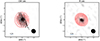 |
Fig. 1. Polarised continuum emission (greyscale) and the 338 GHz continuum contours of CW Leo (left) and R Leo (right). The polarisation peaks at 6.9 and 0.4 mJy beam−1 for CW Leo and R Leo, respectively. The contours are drawn at 0.625%, 1.25%, 2.5%, 5%, 10%, 20%, 40%, and 80% of the peak emission (1.059 and 0.302 Jy beam−1 for CW Leo and R Leo, respectively). The line segments indicate the linear polarisation direction where polarised emission is detected at > 5σP. The uncertainty on the direction is ≲6°. The segments are scaled as indicated by the horizontal bar. The filled ellipses indicate the beam size of the observations. |
Polarisation observational results.
In addition to the continuum polarisation, we measured polarisation at a level of more than 5σP for four molecular transitions around CW Leo and for five molecular transitions around R Leo. The peak fluxes (Ipeak) of the lines for which polarisation was detected as well as the maximum polarisation fraction found in the molecular line maps (Pl, max) are presented in Table 1. As discussed before, the fractional polarisation of the extended emission lines can be affected by filtering out the large-scale structure. We discuss the molecular line polarisation of both sources in more detail in the following subsections.
3.2. CW Leo
We detected significant polarisation around CW Leo for four molecular lines. The emission maps of 12CO J = 3 − 2, CS J = 7 − 6, H13CN J = 4 − 3, and SiS J = 19 − 18 are respectively shown in Figs. 2–5. The maximum fractional polarisation for the four ranges of lines are all between 1% and 2%, but as can be seen in the images, the distribution of the polarised emission and the orientation of the polarisation vectors is different for the different lines. While the polarisation vectors of the H13CN J = 4 − 3 and SiS J = 19 − 18 lines are mainly in the tangential direction, those in the CS J = 7 − 6 line display a direction that is neither tangential nor radial for R < 1.4″. We thus interpreted R = 1.4″ as the radius where the alignment mechanism for CS in particular undergoes a change. The 12CO J = 3 − 2 shows a polarisation structure that is different from all three other lines at larger (R > 1.4″) distances from the centre of the emission and a structure that is consistent with that of CS J = 7 − 6 in the inner envelope. To illustrate the different behaviour of the polarisation direction, we plotted a histogram with the deviation from the tangential direction for all polarisation vectors, shown in Fig. 6 (left), and for those vectors within R < 1.4″ in Fig. 6 (right). All the lines showed a good correspondence of polarisation structure between neighbouring channels despite the fact that the possible effect of the resolved-out large-scale emission is different for the different velocity channels and should be most pronounced closer to the stellar velocity. It is thus unlikely that the observed polarisation structure itself is strongly affected by missing flux.
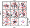 |
Fig. 2. Channel maps of the polarised CO J = 3 − 2 emission around the AGB star CW Leo. The solid red contours indicate the Stokes I total intensity emission at 5%, 10%, 20%, 40%, and 80% of the peak emission (ICO, peak = 17.89 Jy beam−1). The greyscale image is the linearly polarised emission, and the line segments denote the linear polarisation direction where emission is detected at > 5σP. The segments are scaled to the level of fractional polarisation, with the scale indicated in the bottom-right panel. The maximum polarisation is Pl, max = 1.18%. The beam size is denoted in the bottom-right panel, and all panels are labelled with the Vlsr velocity in kilometers per second. The stellar velocity is Vlsr, * = −26.5 km s−1. The dashed blue circles centred on the peak of the CO emission close to the stellar velocity indicates the radius (R ≈ 1.4″) at which we find that the direction of polarisation for CS changes from being neither tangential nor radial to predominantly tangential. |
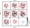 |
Fig. 3. Same as Fig. 2 but for the CS J = 7 − 6 emission around CW Leo. The peak emission is ICS, peak = 18.77 Jy beam−1. The maximum polarisation is Pl, max = 1.74%. |
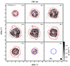 |
Fig. 4. Same as Fig. 2 but for the H13CN J = 4 − 3 emission around CW Leo. The peak emission is IHCN, peak = 38.52 Jy beam−1. The maximum polarisation is Pl, max = 1.62%. |
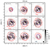 |
Fig. 5. Same as Fig. 2 for the SiS J = 19 − 18 emission around CW Leo. The peak emission is ISiS, peak = 21.01 Jy beam−1. The maximum polarisation is Pl, max = 1.47%. |
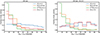 |
Fig. 6. Distribution of polarisation angles with respect to the tangential direction for the emission of CO J = 3 − 2, SiS J = 19 − 18, H13CN J = 4 − 3, and CS J = 7 − 6 around CW Leo. Left: polarisation angles taken from the entire circumstellar envelope emission. Right: polarisation angles for R < 1.4″. |
In Fig. 7 (left), we also present the azimuthally averaged Stokes I, linearly polarised flux, and fractional polarisation for the spectral channel closest to the stellar velocity (Vlsr, CW Leo = −26.5 km s−1). Here we note that for CW Leo, the relative polarisation of the H13CN line is stronger than that of the other lines. As expected, because of the averaging of polarisation structure within the observing beam, all lines show a decrease of fractional polarisation in the central beam. Outside of this, the polarisation fraction of H13CN remains fairly stable around 0.7%, while the average polarisation fraction of 12CO is much lower, but it rises steadily outwards. The fractional polarisation of CS shows a minimum around ∼1.4″, which is consistent with the observed change in morphology at that radius. Finally, the fractional polarisation of SiS behaves somewhat similar to that of H13CN, although it shows a somewhat more pronounced peak around ∼1″ before decreasing to ∼0.2%, and beyond ∼3″, it rises again to peak at ∼0.4%.
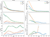 |
Fig. 7. Azimuthally averaged Stokes I (top), polarised intensity (Pl; middle), and polarisation fraction (Pl, frac; bottom), taken in the channel that includes the stellar velocity, for CW Leo (left column) and R Leo (right column). For CW Leo, we show CO J = 3 − 2, SiS J = 19 − 18, H13CN J = 4 − 3, and CS J = 7 − 6. For R Leo, we show CO J = 3 − 2, 29SiO v = 0, J = 4 − 3, and H13CN J = 4 − 3. We did not include the mostly unresolved SiO v = 1 and v = 2, J = 8 − 7 transitions. The profiles of Pl and Pl, frac include the error bars from the azimuthal averaging, and only radial points for which the S/N is greater than five are plotted. Because of the averaging, the polarisation fraction is much less than the maximum fraction detected in the image cubes for each line. Beyond one-third, the ALMA primary beam size (at R ≈ 3.0) systematic errors might start to contribute to the polarisation signal. We note that the units for the polarised intensity are different for the two middle plots for CW Leo (Jy beam−1) and R Leo (mJy beam−1). |
3.3. R Leo
Around R Leo, we found polarisation for 12CO J = 3 − 2, 29SiO v = 0, J = 8 − 7, and H13CN J = 4 − 3, as well as for the v = 1 and v = 2 SiO J = 8 − 7 transitions. Maps for the first three of these are presented in Figs. 8–10. Maps for the vibrationally excited transitions, which likely include maser amplification, are presented in Figs. A.1 and A.2. While the peak level of fractional polarisation of the H13CN around R Leo is similar to that around CW Leo, the peak fractional polarisation of the 12CO is three times higher. As the level of resolved-out flux is larger for the extended envelope of CW Leo, which means that its polarisation fraction is likely more overestimated than for R Leo, the difference between the peak fractional polarisation of the 12CO of both sources is intrinsic. The peak fractional polarisation of the SiO vibrationally excited lines is higher still, with that of the v = 1 transition reaching a level above 30%. This is consistent with previous observations of high frequency SiO masers (e.g. Vlemmings et al. 2011, 2017) and with theoretical predictions (e.g. Lankhaar & Vlemmings 2019; Lankhaar et al. 2024).
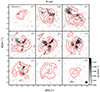 |
Fig. 8. Same as Fig. 2 but for the CO J = 3 − 2 emission around R Leo. The stellar velocity is Vlsr, * = −0.5 km s−1. The peak emission is ICO, peak = 4.66 Jy beam−1. The maximum polarisation is Pl, max = 3.90%. |
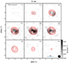 |
Fig. 9. Same as Fig. 2 but for the 29SiO v = 0, J = 8 − 7 emission around R Leo. The peak emission is I29SiO, peak = 8.49 Jy beam−1. The maximum polarisation is Pl, max = 1.57%. |
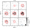 |
Fig. 10. Same as Fig. 2 but for the H13CN J = 4 − 3 emission around R Leo. The peak emission is IHCN, peak = 2.40 Jy beam−1. The maximum polarisation is Pl, max = 1.79%. |
At the same time, the direction of the polarisation vectors of 12CO around R Leo are clearly radial. As illustrated in Fig. 11, the vectors of 29SiO and H13CN are mostly tangential. For the likely masing vibrationally excited states of SiO, the detected polarisation is concentrated towards the central emission peak. This is consistent with the polarised emission originating from masers close to the central star. From positive to negative Vlsr, the polarisation vectors position angle of the v = 1 transition rotates smoothly from 36.4 ± 0.9° to 26.3 ± 1.0°, while that of the v = 2 transition rotates from 47 ± 2° to 22 ± 3°. This indicates a preferred direction of the polarised emission of SiO close to the star, but our angular resolution is not sufficient to draw any stronger conclusions. As noted before, we detected circularly polarised emission of the SiO v = 1 maser line with a (negative) peak flux of Iv = −164 ± 1 mJy beam−1. This corresponds to a circular polarisation percentage of Pv = 1.3%. As the intrinsic maser velocity width is much smaller than the spectral channel width, this percentage will be a lower limit to the actual circular polarisation. Assuming the relation between the SiO maser circular polarisation fraction and the magnetic field strength from Kemball & Diamond (1997), this corresponds to a magnetic field of B ∼ 2 − 3 G in the SiO maser region, which is consistent with previous measurements (Herpin et al. 2006). No circular polarisation above a 5σV level of 5.6 mJy beam−1 was seen for the significantly weaker v = 2 transition.
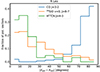 |
Fig. 11. Distribution of polarisation angles with respect to the tangential direction for the emission of CO J = 3 − 2, 29SiO v = 0, J = 8 − 7, and H13CN J = 4 − 3 around R Leo. |
The azimuthally averaged Stokes I, linear polarisation, and fractional polarisation profiles for R Leo are shown in Fig. 7 (right). For the average polarisation, it is also clear that the CO fractional polarisation of R Leo is higher than that of CW Leo, while the H13CN polarisation levels are similar. All lines show the reduced fractional polarisation towards the centre, and for both 29SiO and H13CN, the fractional polarisation appears to peak around R ∼ 1.1″ before slightly decreasing. After this decrease, the fractional polarisation of 29SiO rises sharply towards the outer edge of the 29SiO envelope, while for H13CN the polarised emission becomes too weak to be detectable. The CO polarisation extends further, but the fractional polarisation reduces after peaking at R ∼ 1.7″.
4. Polarised radiative transfer models
We simulated the emergence of polarisation of the emission from different molecules in the circumstellar envelope towards CW Leo and R Leo. The modelling of the line polarisation was performed with the PORTAL (POlarised Radiative Transfer Adapted to Lines) code (Lankhaar & Vlemmings 2020). PORTAL uses the anisotropic intensity approximation (for a thorough discussion, see Lankhaar & Vlemmings 2020) and assumes a dominant symmetry axis for the molecular species of interest. In the case of molecular lines excited in the CSE around evolved stars, the dominant symmetry axis may either be aligned with the magnetic field or the infrared radiation field, which is typically radial. Radiative alignment is expected when radiative interactions occur at a higher rate than the magnetic precession rate (∼s−1 mG−1).
PORTAL maps out the intensity and anisotropy of the radiation field at the resonant frequencies of the molecule under investigation throughout the simulation. The radiative transfer is performed using the converged output of a LIME (version 1.9.5) simulation (Brinch & Hogerheijde 2010). The radiation field (anisotropy) parameters, in conjunction with the magnetic field geometry and density profile, are subsequently used to model the molecular excitation and quantum state alignment throughout the simulation. With the molecular excitation and alignment parameters, one is able to perform a polarised ray-tracing to produce a polarised image of the region of interest.
We modelled the emergence of line polarisation in CO, CS, H13CN, SiS, and 29SiO. These molecules are exposed to a strong radiation field from the central AGB star, and as a result, transitions involving the vibrationally excited states occur at high rates, thus having a high tendency to align the molecular population. We have therefore also included the first vibrationally excited states in modelling the polarised line emission of these molecules. For CO, we included the J = 0 − 40 levels of the first two vibrational states, using the transition frequencies and Einstein coefficients from Li et al. (2015) and the collisional rate coefficients from Castro et al. (2017), assuming an ortho-to-para ratio of 3:1. For CS, we augmented the standard LAMDA datafile (Schöier et al. 2005), which includes collisional rate coefficients of Lique et al. (2006), with the first vibrationally excited state, including only its radiative coupling to the ground state and taking the radiative rates from Li et al. (2015). We used the data from Danilovich et al. (2014) to model H13CN, where we limited the vibrational excitation to the first excited bending mode. For SiS, we augmented the standard LAMDA datafile (Schöier et al. 2005), which includes collisional rate coefficients of Dayou & Balança (2006), with the first vibrationally excited state, including only its radiative coupling to the ground state and taking the radiative rates from (Li et al. 2015). Finally, to model 29SiO, we used the molecular data file from Danilovich et al. (2014).
4.1. Circumstellar envelope models
We performed radiative transfer simulations of circumstellar envelopes of CW Leo and R Leo, using parameterised models of the physical conditions relevant to the radiative transfer towards these objects. The gas density profile was modelled assuming a spherically symmetric envelope of molecular gas and dust expanding at a constant velocity (see e.g. Velilla-Prieto et al. 2019, and references therein)
 (1)
(1)
where Ṁ is the mass-loss rate, r is the radial distance to the star, v∞ is the terminal expansion velocity, and ⟨mg⟩ is the average mass of particles in the gas, for which we adopted 2.35 AMU based on a gas primarily made up of molecular hydrogen and helium. The gas kinetic temperature for CW Leo was assumed to follow the profile (Agúndez et al. 2012)
 (2a)
(2a)
where T* stands for the stellar temperature and R* is the stellar radius. For R Leo, we adopted the kinetic gas temperature profile
 (2b)
(2b)
which is based on the kinetic temperature profile for the similar relatively low mass-loss rate AGB star W Hya (Khouri et al. 2014). For both CW Leo and R Leo, we assumed a lower limit on the gas kinetic temperature of 10 K. The gas temperature was used to compute the velocity dispersion that furthermore contained a contribution from a constant turbulent velocity of 1 km s−1. The dust temperature was assumed to follow
 (3)
(3)
where Rc is the dust condensation radius, Tc is the dust condensation temperature, and qc is the parameterised power-law exponent describing the drop-off of the dust temperature. We did not find a dust temperature profile specifically tailored to R Leo, and we instead adopted the condensation temperature and radius from Ramstedt & Olofsson (2014) and the exponent from an average for M-type stars from Marengo et al. (1997). In LIME, the dust density is determined from the gas density using the gas-to-dust ratio. To enforce the absence of dust within the dust condensation radius, the gas-to-dust mass ratio was set to the arbitrarily high value of 108 for r < Rc. The radiative transfer is highly dependent on the type of dust that is present in the CSE. In the case of C-rich CSEs, such as CW Leo, we adopted the opacities for the amorphous carbon-type dust given by Suh (2000), while for O-rich CSEs, such as R Leo, we adopted the opacities for the silicate type from Suh (1999).
The gas velocity profile was assumed to only have a component in the radial direction. For the radial velocity profile, vexp, we assumed for CW Leo the profile
![Mathematical equation: $$ \begin{aligned} v_{\mathrm{exp} } = {\left\{ \begin{array}{ll} v_{\infty } \left(1-\left[\frac{R_{\mathrm{w} }-r}{R_{\mathrm{w} }}\right]^{2.5}\right) \quad&\mathrm{for} \ r \le R_{\mathrm{w} } \\ v_{\infty } \quad&\mathrm{for} \ r > R_{\mathrm{w} } \end{array}\right.}, \end{aligned} $$](/articles/aa/full_html/2024/06/aa49448-24/aa49448-24-eq6.gif) (4a)
(4a)
where Rw is the wind acceleration radius and v∞ is the terminal wind velocity. We based the CW Leo expansion profile on Agúndez et al. (2012). For R Leo, we adopted a velocity profile similar to W Hya (Khouri et al. 2014):
 (4b)
(4b)
The parameters that were used to represent CW Leo- and R Leo-like circumstellar envelopes are summarised in Table 2. We have attempted to be as representative as possible to the models that exist in the literature but have not adjusted the model parameters for the different distances that were used to derive some of the parameters.
Stellar envelope parameters.
The fractional abundances of the molecules are parameterised according to the following expressions. For the molecular abundances, we adopted a profile (Massalkhi et al. 2020; Saberi et al. 2019)
 (5a)
(5a)
where f0 is the initial abundance at the starting radius of the profile, rp is the characteristic photo-dissociation radius, and α is a parameter to model the steepness of the radial decrease around rp. In Table 3, we present the abundance parameters that were used in our simulations.
Molecular abundance profile parameters.
We used the results of Saberi et al. (2019) for the CO abundance profile. We note that they used the abundance profile
![Mathematical equation: $$ \begin{aligned} f_{\mathrm{mol} }^{\mathrm{Sab} } = f_{{0}}\exp (-\ln (2) {(r/r_{1/2})^{\alpha }}) = f_{{0}}\,\left[\frac{1}{2}\right]^{(r/r_{1/2})^{\alpha }}, \end{aligned} $$](/articles/aa/full_html/2024/06/aa49448-24/aa49448-24-eq9.gif) (5b)
(5b)
for their parameterization. We adopted their values for the photo-dissociation radius to the profile we employed (Eq. (5a)), using rp = [ln(2)]−1/αr1/2.
4.2. Line polarisation simulations: CW Leo
We modelled the polarised emission from the ALMA Band 7 transitions of the molecules CO, H13CN, SiS, and CS towards a model of a circumstellar envelope with parameters representing the CSE towards the AGB star CW Leo. The polarised emission of the molecular lines is in the direction of the molecular alignment axis. In the interstellar medium, this axis is generally aligned with respect to the magnetic field direction, as precession around the magnetic field is fast relative to the other directional radiative interactions. However, in the CSEs that we investigated, the molecular lines of interest are excited in a region close to a strong stellar radiation source, thus inducing strong vibrational radiative interactions. It is possible that the stellar radiation field, which is typically in the radial direction of the CSE, determines the molecular alignment axis if the radiative transition rates exceed the magnetic precession rate.
In Fig. 12, as a first step to investigate the dominant axis of alignment, we compare the upper levels of the investigated transitions, the radiative interaction rates to the magnetic precession rate, as a function of the distance to the central stellar object. The magnetic precession rate depends on the magnetic field strength. We give the magnetic precession rate assuming a surface magnetic field of Bsurf = 1 G, a B ∝ R−2 and a B ∝ R−3 distance relation, and Bsurf = 1 mG with a B ∝ R−1 distance relation. Whilst the magnetic precession rate is unknown, it is striking that radiative interaction rates of the molecules CS, H13CN, and SiS far exceed the radiative interaction rates of CO. Indeed, assuming a magnetic field B = 1 G (R/R*)−3, as would be typical for a dipole magnetic field, we predicted that CO molecules align themselves to the magnetic field, whilst CS, H13CN, and SiS align to the (radially directed) radiation field.
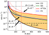 |
Fig. 12. Comparison of the radiative interaction (solid lines) and magnetic precession rates (dash-dotted lines) of the investigated molecules toward CW Leo. The magnetic precession rates are given for magnetic fields B = Bsurf(R/Rstar)−q, adopting q = 1, q = 2 and 3, where for q = 1 a Bsurf = 1 mG was adopted, while for q = 2 and 3, Bsurf = 1 G was adopted. The black curve composed of long dashes indicates the expected magnetic precession rates that explain the polarisation morphology of CS, CO, and H13CN within 1.4″. The horizontal black dotted and dash-dotted lines indicate the molecular magnetic precession rates at 1 mG and 1 μG, respectively. The vertical black and red dotted lines indicate telescope resolution and the 1.4″ radius where a polarisation morphology change was observed (see Sect. 3.2). The orange coloured region indicates the magnetic field strengths where CO would be aligned to the magnetic field but H13CN would be aligned in the radial direction along the stellar radiation field. |
Concurrently, Figs. 2–5 show an intricate polarisation morphology for CO consistent with a non-radial alignment direction. The polarisation vectors in the CS, H13CN, and SiS observations tend to be tangential in regions beyond 1.4″, which is consistent with the radial alignment direction of the molecules. For offsets less than 1.4″, a transition into a different polarisation morphology seems to emerge for CS and, to a lesser degree, SiS. Strikingly, this polarisation morphology seems to agree with the morphology obtained from CO. We took this as an indication that CO is aligned with the magnetic field throughout the CSE and that for offsets less than 1.4″, the magnetic field is also the dominant alignment direction for CS and SiS. We found that H13CN is aligned to the radiation field throughout the CSE, while CS and SiS are radiatively aligned for R > 1.4″. The different alignment properties of the molecules allowed us to estimate the magnetic field from the radiative interaction rates. For the entire (observed) CSE, we found that the magnetic field has to lie in the orange highlighted region in Fig. 12, whereas the different alignment properties for R < 1.4″ suggest magnetic field strengths of ≳20 mG [R/(1.4″)]−2 = 80 mG [R/R*]−2 for R < 1.4″.
In Fig. 13, we present PORTAL simulations of the transition lines of CS, H13CN, and SiS excited towards CW Leo. For these simulations, we assumed the alignment axis to lie in the radial direction, which is the direction expected when molecules are radiatively aligned to the central stellar radiation field. Polarisation intensities and fractions are roughly consistent with the observations for CS and SiS. For H13CN, the PORTAL simulations predict a larger region where emission is polarised at a detectable level, as well as a azimuthally averaged polarisation fraction that peaks at ∼4%. This is approximately two times higher than that seen in Fig. 7. For H13CN, we predicted a tangential polarisation morphology throughout the emission region, which is consistent with observations. Likewise, for SiS, we predicted a tangential polarisation morphology, which at offsets in excess of 1.4″ is consistent with the observations. The CS polarisation is tangential in the inner regions but also shows a 90° flip to a radial morphology in a region with relatively low polarisation yields. For offsets of less than 1.4″, we correctly predicted the tangential polarisation morphology of H13CN, while the predicted polarisation morphology of CS and SiS begins to diverge from the observed polarisation morphology. We suggest that this is an additional indication for a non-radial alignment in play that is close to the central star.
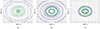 |
Fig. 13. Predicted polarised intensity contours (labelled in units of mJy beam−1) overlaid with line segments that indicate the polarisation of (a) H13CN, (b) CS, and (c) SiS emission emerging from a CSE representative of CW Leo. The polarised intensity is given at the systemic velocity channel. The symmetry axis of the molecules was chosen in the radial direction, representative of radiative alignment. The simulated data has been convolved with the synthesised beam from the observations. The panels correspond to the emission in a velocity channel centred on the stellar velocity. |
In Fig. 14, we present PORTAL simulations of CO emission excited towards CW Leo. For these simulations, we assumed the alignment axis to be determined by a dipole magnetic field. We assumed the dipole to be directed with a position angle of 125°, as was suggested by Andersson et al. (2024), and we assumed it to be inclined at 45°. Towards the systemic velocity, we predicted the polarisation morphology to adhere to a dipolar morphology, while at larger velocity offsets, the polarisation geometry becomes more intricate, with pronounced asymmetry between either sides of the dipole position angle. In addition, larger polarisation degrees are expected at large velocity offsets. Comparing the predicted polarisation morphology to the observed polarisation morphology in CO, we found only modest agreement. In Fig. B.1, we further investigate the polarisation signature of a toroidal magnetic field in the spectral lines of CO. Similar to the dipolar configuration, the symmetry axis is inclined at 45°, while the position angle is at 125°. As was the case for the dipolar polarisation morphology, only modest agreement with the observations was found. This likely indicates that the morphology of the magnetic field in the envelope of CW Leo cannot be described by a simple magnetic field geometry.
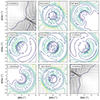 |
Fig. 14. Same as Fig. 13 but for a range of velocity channels of CO emission emerging from a CSE representative of CW Leo. The symmetry axis of the molecules was chosen to be along the magnetic field, which we assumed to be a dipole field with a position angle of 125° and inclination of 45°. For this figure, the line segments are scaled according to the polarisation fraction. |
4.3. Line polarisation simulations: R Leo
We modelled the polarised emission from the ALMA Band 7 transitions of the molecules CO, H13CN, and 29SiO towards a model of a circumstellar envelope with parameters representing the CSE towards the AGB star R Leo. As was done for CW Leo, as a first step to investigating the dominant axis of alignment, in Fig. 15 we compare the upper levels of the investigated transitions, the radiative interaction rates to the magnetic precession rate, as a function of the distance to the central stellar object. The magnetic precession rate depends on the magnetic field strength. Magnetic precession rates are given for magnetic fields B = Bsurf(R/Rstar)−q, adopting q = 1, q = 2 and 3, where for q = 1 a Bsurf = 1 mG was adopted, while for q = 2 and 3, Bsurf = 1 G was adopted. We found low rates of radiative interactions for all investigated molecules. We also found that beyond 100 AU, a magnetic field in excess of 10 μG would determine the alignment direction.
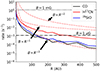 |
Fig. 15. Comparison of the radiative interaction (solid lines) and magnetic precession rates (dash-dotted lines) of the investigated molecules towards R Leo. Magnetic precession rates are given for magnetic fields B = Bsurf(R/Rstar)−q, adopting q = 2 and 3. The black dotted and dash-dotted lines indicate the molecular magnetic precession rates at 1 mG and 1 μG, respectively. |
Due to the low radiative interaction rates, we expected that the magnetic field determines the symmetry axes of the investigated molecules. Thus, the polarisation morphologies seen towards R Leo and reported in Figs. 8 and 9 suggest a radial magnetic field that is likely the result of the influence of advection due to the outflow. In Fig. 16, we present PORTAL simulations of the transition lines of CO, H13CN, and 29SiO excited towards R Leo, assuming a radial symmetry axis. We found significant (> 0.5%) polarisation for the CO in regions within 2.5″, while for H13CN and 29SiO, significant polarisation was found within 1.5″.
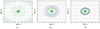 |
Fig. 16. Same as Fig. 13 but for the (a) CO, (b) H13CN, and (c) 29SiO emission emerging from a CSE representative of R Leo. The polarised intensity is given at the systemic velocity channel. The symmetry axis of the molecules was chosen in the radial direction. |
The predicted polarisation morphology appears to be consistent with the observations. Crucially, as in the observations, for CO, we predicted a radial polarisation morphology, while for H13CN and 29SiO the polarisation morphology is predicted to be tangential. The regions with significant polarisation also agree with the observations. In the observations, the polarisation degree of CO throughout the region varies strongly, which is something we did not find in our simulations. It should be noted, though, that the total intensity shows a variable emission pattern as well, which is likely due to an inhomogeneous outflow. Such clumpy structures may locally introduce an additional radiation anisotropy that results in local enhancements of the polarisation degrees. Indeed, the regions showing intensity fluctuations in the CO observations of R Leo seem to be associated with high degrees of polarisation.
5. Discussion
5.1. Comparison with previous observations
The molecular line polarisation arising from the GK effect has previously been observed for both CW Leo and R Leo respectively with the Submillimeter Array (SMA; Girart et al. 2012) and the Combined Array for Research in Millimeter-wave Astronomy (CARMA; Huang et al. 2020). The SMA CW Leo observations targeted the same molecular transitions and detected polarisation up to a level of ∼6σ at a spatial resolution of ∼1.5 × 3″. Those observations had a spectral resolution of 20 km s−1 for CO J = 3 − 2, CS J = 7 − 6, and SiS J = 19 − 18. The very different spatial and spectral resolutions as well as the limited sensitivity of the SMA observations made a direct comparison difficult. The peak polarisation levels in the SMA observations were on the order of ∼2% for CO and SiS and of ∼4% for the CS. The SiS (in the right panel of Fig. 2 in Girart et al. 2012 but wrongly identified as the middle panel in the caption) shows the same tangential morphology as seen in our observations. The polarisation of the CS (in the middle panel of Fig. 2 in Girart et al. 2012 but wrongly identified as the right panel) is, however, stronger in the SMA observations and located in a region outside of the area where the polarisation is detected in the ALMA observations. The CO polarisation was limited to a single large beam in the SMA observations and cannot be compared directly, even if the fractional polarisation is similar. The differences between the SMA and ALMA observations can likely be attributed to the relatively low significance of the polarisation signal in the SMA observations as well as the differences in resolution and spatial filtering of the emission.
The CARMA observations of R Leo (Huang et al. 2020) included the CO J = 2 − 1 and SiO v = 1, J = 5 − 4 maser line at a spatial resolution of ∼4 × 5″ and a spectral resolution of 1 km s−1. The CO polarisation was detected at a level of ∼6σ and a high fractional polarisation level of ∼10%. The fractional polarisation is expected to be higher at the lower-J transitions of CO, but considering the low significance and difference in spatial filtering, we could not make a relevant comparison. The polarisation vector direction shown in Huang et al. (2020) is consistent with a radial polarisation morphology. The SiO maser was detected with a fractional polarisation of ∼35%, similar to the level measured in our observations for the J = 8 − 7 transition. Although the direction of the polarisation reported in Table 3 of Huang et al. (2020) for the SiO maser is different, the direction seen in their Fig. 5 is fully consistent with the direction shown in our Fig. A.1. The good correspondence between the direction of polarisation of the two different maser transitions further supports the existence of a preferred magnetic field direction in the SiO maser region close to the star. Observations of the Zeeman splitting by Herpin et al. (2006) of SiO v = 1, J = 2 − 1 indicate a field strength in the SiO maser region between B = 4 − 5 G.
Continuum polarisation has also been observed in the extended dust envelope around CW Leo using SOFIA (Andersson et al. 2022) and SCUBA-2 (Andersson et al. 2024). The ALMA observations cover much less than a single, central beam of the JCTM SCUBA-2 observations. We adopted the dipole model described in Andersson et al. (2024) in our model shown in Fig. 14, but because of the large difference in scales, we could not make more than a qualitative comparison. It appears that at the scales probed by ALMA, the magnetic field morphology is more complex than a dipole field. Our continuum polarisation direction, as well as the dominant direction of the CO polarisation towards the star, is consistent with the single SCUBA-2 vector in the region probed by the ALMA observations. Unfortunately, the spatial interferometric filtering and the low surface brightness in the extended envelope at ALMA resolution did not allow us to compare the extended emission between SCUBA-2 (and SOFIA) and ALMA, even with mosaicked observations.
5.2. Anisotropic resonant scattering
In addition to the generation of linear polarisation due to the GK effect when emission passes through a magnetised molecular region, linear polarisation can also be converted into circular polarisation in an effect known as anisotropic resonant scattering (Houde et al. 2013, 2022). As a result, the linear polarisation might no longer trace the magnetic field direction.
Since the circular polarisation of the extended lines in our observations is affected by the beam squint of the ALMA antennas (see also Teague et al. 2021), we could not directly investigate anisotropic resonance scattering through a study of the circular polarisation. As argued in Vlemmings & Tafoya (2023), the possible anisotropic scattering of molecular lines in a circumstellar envelope is likely limited to that arising from the emitting region itself since the limits imposed by photo-dissociation and large velocity gradients severely reduce the available molecular column density of the foreground. In Chamma et al. (2018), the SMA polarisation observations of CW Leo were analysed, and it was concluded that significant anisotropic resonant scattering was present in all of the lines also observed with ALMA. This was based on the detection of several percent of circular polarisation in different regions of the circumstellar envelope. However, this would result in significant rotation (and complete depolarisation in some cases) of the linear polarisation vectors, with strong variation across the envelope. This would have ruled out the detection of the structured radial or tangential polarisation morphology we observed. However, we detected no sign of this behaviour in our linear polarisation maps of the CS, SiS, and H13CN. This led us to conclude that the circular polarisation detected towards CW Leo in Chamma et al. (2018) is not the results of anisotropic resonant scattering but is rather an instrumental effect. Since we did not appear to see the signatures of vector rotation towards most of the lines, we concluded that anisotropic resonant scattering likely does not affect the polarisation of our sources. A firm conclusion can only be reached when high-quality circular polarisation observations become available.
5.3. Magnetic field strength: Structure-function analysis
By assuming that the polarisation vectors of the CO J = 3 − 2 transition correspond to the large-scale magnetic field around CW Leo, we could use a structure-function analysis, often used for magnetic field studies of star-forming regions, to calculate the ratio between the turbulent and mean large-scale magnetic field strength (e.g. Hildebrand et al. 2009; Houde et al. 2009). In our analysis, we followed the equations from Koch et al. (2010) and the steps described in Vlemmings & Tafoya (2023).
Under the assumption that the turbulent field arises from transverse Alfvén waves in an environment with isotropic and incompressible turbulence in which the magnetic field is frozen into the gas, the ratio between the turbulent (Bt) and large-scale magnetic field component B0 is equal to the ratio between the turbulent line width σν and the Alfvén velocity  . Here, ρ is the density of the gas. Assuming an average density and turbulent velocity of the emitting region of the CO gas, we could then derive an estimate for the strength of the plane-of-sky component of the large-scale magnetic field. In the case that the magnetic field is not fully frozen in the gas, which is likely the case around CW Leo considering the observed morphology of the magnetic field, the derived field strength should be considered a lower limit.
Figure 17 shows the result of the structure-function analysis for the central velocity channel of the CO emission around CW Leo. The dispersion of the polarisation vectors is shown to steadily increase from the small scales until asymptotically approaching a plateau of ∼70° in a behaviour of the structure function similar to that observed for several star-forming regions (e.g. Dall’Olio et al. 2019). The structure function can be fit using the equation from Koch et al. (2010) within ≲2″, which is the characteristic length scale for variations in the large-scale magnetic field component. We found that the ratio between the turbulent and large-scale magnetic field component is  . Similar to Vlemmings & Tafoya (2023), this means that we can write the strength of the large-scale magnetic field strength as
 (6)
(6)
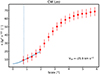 |
Fig. 17. Dispersion of the polarisation vectors (the square root of the second-order structure function), binned to the Nyquist-sampled resolution, for the central velocity channel of the CO J = 3 − 2 polarised emission around CW Leo. The error bars indicate the variance in each bin. The vertical dotted line indicates the size of the beam’s major axis. The solid line indicates the fit of the structure-function analysis described in the text. |
with the average H2 number density, nH2, in the CO region in units of particles per centimeter cubed (cm−3) and the typical turbulent velocity, vt, in kilometers per second. The adopted density corresponds to a radius of ∼250 au. Using Eq. (1) and the CW Leo mass-loss rate and expansion velocity, we can also describe the magnetic field as a function of radius in the region of the ALMA observations (between the Nyquist sampled beam and maximum recoverable scale) as B = 107 × (50/r) mG between r = 50 and 485 au. The error on the derived field strength is completely dominated by the uncertainty in the average number density and the assumption of magnetic flux freezing. A further source of uncertainty is the effect of limited angular resolution and spatial filtering (Houde et al. 2016). Following the approach outlined in Vlemmings & Tafoya (2023), the number of independent turbulent cells (N) probed by our observations was estimated using the formula from Houde et al. (2016):
 (7)
(7)
We used the approximation that the correlation length, δ, is set by the typical clump size rc ∝ r0.8, while the depth of the observed molecular layer along the line of sight, Δ′, is estimated from the total size of the CO envelope divided by the number of channels (for a derivation of both of these, see Vlemmings & Tafoya 2023). This yielded δ ∼ 300 au and Δ′∼500 au. The parameter W1 ≈ 40 au is the radius of the interferometric beam. Hence, we found N ∼ 1.2. According to Houde et al. (2016), the ratio between the turbulent and large-scale magnetic field strengths scales with  . This means that our derived magnetic field strength does not require a significant correction.
An analysis of the other velocity channels for which sufficient independent polarisation vectors were measured yielded similar field strengths to within 30%. The field strength is two to ten times higher than the line-of-sight magnetic field strength of |B|||∼2 − 9 mG estimated from Zeeman splitting of CN in the outer part (R ∼ 2500 au) of the envelope of CW Leo (Duthu et al. 2017). Since we measured the (plane-of-sky) field component in CO much closer to the star (R ∼ 250 au), the comparison between the CO estimates and possible CN Zeeman measurements implies that the magnetic field strength beyond R ∼ 250 au decreases outwards as R−q with 0.3 < q < 1.0. Taking into account the large uncertainties, this is only marginally consistent with a dominating toroidal magnetic field component at these radii (q = 1). A magnetic field frozen into the spherically expanding gas or a solar-type magnetic field (q = 2) as well as a dipole-shaped or radial magnetic field (q = 3) appear to be ruled out.
5.4. Magnetic field strength: Molecular alignment
As described in Sect. 4 and shown in Figs. 12 and 15, a comparison between the radiative excitation and magnetic precession rates for various magnetic tracers throughout the circumstellar envelope can also be used to derive an estimate of the magnetic field strength.
We present such a comparison in Fig. 18. For the relatively low-density outflow around R Leo, it is clear that the magnetic precession rate dominates the radiative rates of our observed molecular lines throughout the entire envelope, even for a very low (∼10 μG) magnetic field strength. As described in Sect. 4.3, a radial magnetic field can reproduce all observed lines. This would imply that, around R Leo, the magnetic field in much of the envelope is coupled to the outflow but that the kinetic outflow energy dominates the magnetic energy, resulting in the magnetic field lines being stretched by the predominantly radial outflow.
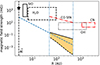 |
Fig. 18. Magnetic field strength in AGB circumstellar envelopes as a function of radial distance. The black boxes indicate the literature values reported from maser measurements (e.g. Herpin et al. 2006; Leal-Ferreira et al. 2013; Vlemmings et al. 2005; Rudnitski et al. 2010). The black star indicates the surface magnetic field measurement for the star χ Cyg (Lèbre et al. 2014). The measurements for CW Leo are indicated in red. These are the CN Zeeman measurements from Duthu et al. (2017, red dash-dotted box) and the CO structure-function analysis result reported in Sect. 5.3 (red dashed-dotted line). For the CO result, we used the relation between nH2 and R for the range of radii probed by the ALMA observations (Eq. (6)). This range is indicated by the vertical dotted lines. The stellar surface is indicated by the long-dashed vertical line. For the region probed by ALMA around CW Leo, we indicate in orange the lower (dashed) and upper (solid) magnetic field limits based on the analysis of the 12CO and H13CN radiative interaction rates. The relation between radius and magnetic field strength that fits the observations and modelled radiative rates described in Sect. 4.2 is presented as the blue dashed relation (we extrapolated out to the maximum scale probed with the ALMA polarisation observations). It is clear that this relation is not in agreement with the other magnetic field strength observations. |
For the much denser envelope of CW Leo, the different behaviour of the various molecular tracers places constraints on the magnetic field strength throughout the envelope. However, these constraints are not consistent with either the magnetic field strength determined from the structure-function analysis of the CO emission or the CN Zeeman measurements in the outer envelope (Duthu et al. 2017). Specifically, the fact that beyond ∼1.4″, the CS, SiS, and H13CN all apparently trace the direction imposed by the radiation field while the CO still traces the magnetic field seems to rule out a magnetic field strength of ≳20 μG at R ∼ 170 au and beyond. As discussed previously, the CN Zeeman observations appear to indicate |B|||∼2 − 9 mG at ∼2500 au, and the CO structure-function analysis implies |B⊥|∼19 mG at ∼250 au. Under the conditions of such a magnetic field, CS, SiS, and H13CN should also be aligned with the magnetic field in the outer envelope. One possible solution to this discrepancy is if our molecular analysis did not include all relevant molecular transitions through which the molecular alignment can occur. Should the radiative molecular alignment for the species we observed be more effective in, for example, higher vibrational transitions that were not considered, the radiative alignment rates in our models would increase. This would allow for a stronger magnetic field while maintaining the radiative alignment of CS, SiS, and H13CN in the outer envelope.
6. Conclusions
We have presented a detailed analysis of the molecular line polarisation observed with ALMA in the circumstellar envelopes of the C-type AGB star CW Leo and the M-type AGB star R Leo. In both sources, we detected line polarisation of multiple molecular lines, with fractions ranging from 1.18% for 12CO to 32.4% for one of the masing SiO lines. We also detected polarisation of the continuum, but since most dust continuum emission is filtered out by the interferometric observations, this was limited to a single beam towards the stars. Around CW Leo, the CO polarisation likely traces a complex large-scale magnetic field. Within R = 1.4″ ≈ 170 au, CS traces the same structure. The polarisation vectors of SiS and H13CN, as well as those of CS beyond 170 au, are predominantly tangential, indicating molecular alignment due to the radiation field. A structure-function analysis of the CO revealed a plane-of-sky magnetic field of ∼19 mG at R = 250 au, which would be consistent with the values obtained from CN Zeeman observations (Duthu et al. 2017). These values, however, are too high to explain the alignment of CS, SiS, and H13CN with the radiation field in the outer envelope. Additional modelling and observations are needed to solve this discrepancy. Around R Leo, the observed polarisation morphology of the CO, H13CN, and 29SiO can be explained by a large-scale magnetic field that is radially advected by the outflow. The observations and modelling presented here show that polarisation observations of multiple molecular species can be a powerful tool to determine not only the magnetic field but also the behaviour of the radiation field throughout circumstellar envelopes.
Acknowledgments
B.L. acknowledges VR support under grant No. 2021-00339. This paper makes use of the following ALMA data: ADS/JAO.ALMA#2016.1.00251.S. ALMA is a partnership of ESO (representing its member states), NSF (USA) and NINS (Japan), together with NRC (Canada), NSC and ASIAA (Taiwan), and KASI (Republic of Korea), in cooperation with the Republic of Chile. The Joint ALMA Observatory is operated by ESO, AUI/NRAO and NAOJ. The project leading to this publication has received support from ORP, that is funded by the European Union’s Horizon 2020 research and innovation programme under grant agreement No. 101004719 [ORP]. L.V.-P. acknowledges support from the grant PID2020-117034RJ-I00 funded by the Spanish MCIN/AEI/10.13039/501100011033. The computations were enabled by resources provided by Chalmers e-Commons at Chalmers. We also acknowledge support from the Nordic ALMA Regional Centre (ARC) node based at Onsala Space Observatory. The Nordic ARC node is funded through Swedish Research Council grant No 2017-00648.
References
- Agúndez, M., Fonfría, J. P., Cernicharo, J., et al. 2012, A&A, 543, A48 [NASA ADS] [CrossRef] [EDP Sciences] [Google Scholar]
- Andersson, B.-G., Lopez-Rodriguez, E., Medan, I., et al. 2022, ApJ, 931, 80 [NASA ADS] [CrossRef] [Google Scholar]
- Andersson, B. G., Karoly, J., Bastien, P., et al. 2024, ApJ, 963, 76 [NASA ADS] [CrossRef] [Google Scholar]
- Andriantsaralaza, M., Ramstedt, S., Vlemmings, W. H. T., et al. 2022, A&A, 667, A74 [NASA ADS] [CrossRef] [EDP Sciences] [Google Scholar]
- Beuther, H., Vlemmings, W. H. T., Rao, R., et al. 2010, ApJ, 724, L113 [NASA ADS] [CrossRef] [Google Scholar]
- Brinch, C., & Hogerheijde, M. R. 2010, A&A, 523, A25 [NASA ADS] [CrossRef] [EDP Sciences] [Google Scholar]
- Castro, C., Doan, K., Klemka, M., et al. 2017, Mol. Astrophys., 6, 47 [NASA ADS] [CrossRef] [Google Scholar]
- Chamma, M. A., Houde, M., Girart, J. M., et al. 2018, MNRAS, 480, 3123 [CrossRef] [Google Scholar]
- Cortes, P. C., Crutcher, R. M., & Watson, W. D. 2005, ApJ, 628, 780 [NASA ADS] [CrossRef] [Google Scholar]
- Dall’Olio, D., Vlemmings, W. H. T., Persson, M. V., et al. 2019, A&A, 626, A36 [NASA ADS] [CrossRef] [EDP Sciences] [Google Scholar]
- Danilovich, T., Bergman, P., Justtanont, K., et al. 2014, A&A, 569, A76 [NASA ADS] [CrossRef] [EDP Sciences] [Google Scholar]
- Dayou, F., & Balança, C. 2006, A&A, 459, 297 [NASA ADS] [CrossRef] [EDP Sciences] [Google Scholar]
- De Beck, E., & Olofsson, H. 2018, A&A, 615, A8 [NASA ADS] [CrossRef] [EDP Sciences] [Google Scholar]
- Duthu, A., Herpin, F., Wiesemeyer, H., et al. 2017, A&A, 604, A12 [NASA ADS] [CrossRef] [EDP Sciences] [Google Scholar]
- Gaia Collaboration (Brown, A. G. A., et al.) 2018, A&A, 616, A1 [NASA ADS] [CrossRef] [EDP Sciences] [Google Scholar]
- Gaia Collaboration (Brown, A. G. A., et al.) 2021, A&A, 649, A1 [NASA ADS] [CrossRef] [EDP Sciences] [Google Scholar]
- Girart, J. M., Patel, N., Vlemmings, W. H. T., et al. 2012, ApJ, 751, L20 [NASA ADS] [CrossRef] [Google Scholar]
- Goldreich, P., & Kylafis, N. D. 1982, ApJ, 253, 606 [NASA ADS] [CrossRef] [Google Scholar]
- Gonidakis, I., Chapman, J. M., Deacon, R. M., et al. 2014, MNRAS, 443, 3819 [NASA ADS] [CrossRef] [Google Scholar]
- Groenewegen, M. A. T., Barlow, M. J., Blommaert, J. A. D. L., et al. 2012, A&A, 543, L8 [NASA ADS] [CrossRef] [EDP Sciences] [Google Scholar]
- Guélin, M., Patel, N. A., Bremer, M., et al. 2018, A&A, 610, A4 [NASA ADS] [CrossRef] [EDP Sciences] [Google Scholar]
- Haniff, C. A., Scholz, M., & Tuthill, P. G. 1995, MNRAS, 276, 640 [NASA ADS] [CrossRef] [Google Scholar]
- Herpin, F., Baudry, A., Thum, C., et al. 2006, A&A, 450, 667 [NASA ADS] [CrossRef] [EDP Sciences] [Google Scholar]
- Hildebrand, R. H., Kirby, L., Dotson, J. L., et al. 2009, ApJ, 696, 567 [NASA ADS] [CrossRef] [Google Scholar]
- Höfner, S., & Olofsson, H. 2018, A&ARv, 26, 1 [Google Scholar]
- Houde, M., Vaillancourt, J. E., Hildebrand, R. H., et al. 2009, ApJ, 706, 1504 [NASA ADS] [CrossRef] [Google Scholar]
- Houde, M., Hezareh, T., Jones, S., et al. 2013, ApJ, 764, 24 [NASA ADS] [CrossRef] [Google Scholar]
- Houde, M., Hull, C. L. H., Plambeck, R. L., et al. 2016, ApJ, 820, 38 [NASA ADS] [CrossRef] [Google Scholar]
- Houde, M., Lankhaar, B., Rajabi, F., et al. 2022, MNRAS, 511, 295 [CrossRef] [Google Scholar]
- Huang, K.-Y., Kemball, A. J., Vlemmings, W. H. T., et al. 2020, ApJ, 899, 152 [NASA ADS] [CrossRef] [Google Scholar]
- Hull, C. L. H., Cortes, P. C., Gouellec, V. J. M. L., et al. 2020, PASP, 132, 094501 [NASA ADS] [CrossRef] [Google Scholar]
- Kemball, A. J., & Diamond, P. J. 1997, ApJ, 481, L111 [NASA ADS] [CrossRef] [Google Scholar]
- Khouri, T., de Koter, A., Decin, L., et al. 2014, A&A, 570, A67 [NASA ADS] [CrossRef] [EDP Sciences] [Google Scholar]
- Koch, P. M., Tang, Y.-W., & Ho, P. T. P. 2010, ApJ, 721, 815 [NASA ADS] [CrossRef] [Google Scholar]
- Lankhaar, B., & Vlemmings, W. 2019, A&A, 628, A14 [NASA ADS] [CrossRef] [EDP Sciences] [Google Scholar]
- Lankhaar, B., & Vlemmings, W. 2020, A&A, 636, A14 [NASA ADS] [CrossRef] [EDP Sciences] [Google Scholar]
- Lankhaar, B., Surcis, G., Vlemmings, W., & Impellizzeri, V. 2024, A&A, 683, A117 [NASA ADS] [CrossRef] [EDP Sciences] [Google Scholar]
- Leal-Ferreira, M. L., Vlemmings, W. H. T., Kemball, A., et al. 2013, A&A, 554, A134 [NASA ADS] [CrossRef] [EDP Sciences] [Google Scholar]
- Leão, I. C., de Laverny, P., Mékarnia, D., et al. 2006, A&A, 455, 187 [NASA ADS] [CrossRef] [EDP Sciences] [Google Scholar]
- Lèbre, A., Aurière, M., Fabas, N., et al. 2014, A&A, 561, A85 [NASA ADS] [CrossRef] [EDP Sciences] [Google Scholar]
- Li, H.-B., & Henning, T. 2011, Nature, 479, 499 [NASA ADS] [CrossRef] [Google Scholar]
- Li, G., Gordon, I. E., Rothman, L. S., et al. 2015, ApJS, 216, 15 [NASA ADS] [CrossRef] [Google Scholar]
- Lique, F., Spielfiedel, A., & Cernicharo, J. 2006, A&A, 451, 1125 [NASA ADS] [CrossRef] [EDP Sciences] [Google Scholar]
- Marengo, M., Canil, G., Silvestro, G., et al. 1997, A&A, 322, 924 [NASA ADS] [Google Scholar]
- Massalkhi, S., Agúndez, M., Cernicharo, J., et al. 2019, A&A, 628, A62 [CrossRef] [EDP Sciences] [PubMed] [Google Scholar]
- Massalkhi, S., Agúndez, M., Cernicharo, J., et al. 2020, A&A, 641, A57 [NASA ADS] [CrossRef] [EDP Sciences] [Google Scholar]
- Mauron, N., & Huggins, P. J. 2000, A&A, 359, 707 [Google Scholar]
- McGuire, B. A. 2018, ApJS, 239, 17 [Google Scholar]
- Morris, M., Lucas, R., & Omont, A. 1985, A&A, 142, 107 [NASA ADS] [Google Scholar]
- Nagai, H., Nakanishi, K., Paladino, R., et al. 2016, ApJ, 824, 132 [NASA ADS] [CrossRef] [Google Scholar]
- Perez-Sanchez, A. F., Vlemmings, W. H. T., Tafoya, D., et al. 2013, MNRAS, 436, L79 [NASA ADS] [CrossRef] [Google Scholar]
- Ramstedt, S., & Olofsson, H. 2014, A&A, 566, A145 [NASA ADS] [CrossRef] [EDP Sciences] [Google Scholar]
- Ramstedt, S., Vlemmings, W. H. T., Doan, L., et al. 2020, A&A, 640, A133 [EDP Sciences] [Google Scholar]
- Rudnitski, G. M., Pashchenko, M. I., & Colom, P. 2010, Astron. Rep., 54, 400 [NASA ADS] [CrossRef] [Google Scholar]
- Saberi, M., Vlemmings, W., & De Beck, E. 2019, A&A, 625, A81 [NASA ADS] [CrossRef] [EDP Sciences] [Google Scholar]
- Schöier, F. L., van der Tak, F. F. S., van Dishoeck, E. F., et al. 2005, A&A, 432, 369 [Google Scholar]
- Schöier, F. L., Ramstedt, S., Olofsson, H., et al. 2013, A&A, 550, A78 [Google Scholar]
- Stephens, I. W., Fernández-López, M., Li, Z.-Y., et al. 2020, ApJ, 901, 71 [CrossRef] [Google Scholar]
- Suh, K.-W. 1999, MNRAS, 304, 389 [NASA ADS] [CrossRef] [Google Scholar]
- Suh, K.-W. 2000, MNRAS, 315, 740 [NASA ADS] [CrossRef] [Google Scholar]
- Teague, R., Hull, C. L. H., Guilloteau, S., et al. 2021, ApJ, 922, 139 [NASA ADS] [CrossRef] [Google Scholar]
- Teyssier, D., Hernandez, R., Bujarrabal, V., et al. 2006, A&A, 450, 167 [NASA ADS] [CrossRef] [EDP Sciences] [Google Scholar]
- Velilla-Prieto, L., Cernicharo, J., Agúndez, M., et al. 2019, A&A, 629, A146 [NASA ADS] [CrossRef] [EDP Sciences] [Google Scholar]
- Velilla-Prieto, L., Fonfría, J. P., Agúndez, M., et al. 2023, Nature, 617, 696 [NASA ADS] [CrossRef] [Google Scholar]
- Vlemmings, W. 2019, IAU Symp., 343, 19 [NASA ADS] [Google Scholar]
- Vlemmings, W. H. T., & Tafoya, D. 2023, A&A, 671, A117 [NASA ADS] [CrossRef] [EDP Sciences] [Google Scholar]
- Vlemmings, W. H. T., Diamond, P. J., & van Langevelde, H. J. 2002, A&A, 394, 589 [NASA ADS] [CrossRef] [EDP Sciences] [Google Scholar]
- Vlemmings, W. H. T., van Langevelde, H. J., & Diamond, P. J. 2005, A&A, 434, 1029 [NASA ADS] [CrossRef] [EDP Sciences] [Google Scholar]
- Vlemmings, W. H. T., Diamond, P. J., & Imai, H. 2006, Nature, 440, 58 [Google Scholar]
- Vlemmings, W. H. T., Humphreys, E. M. L., & Franco-Hernández, R. 2011, ApJ, 728, 149 [Google Scholar]
- Vlemmings, W. H. T., Ramstedt, S., Rao, R., et al. 2012, A&A, 540, L3 [NASA ADS] [CrossRef] [EDP Sciences] [Google Scholar]
- Vlemmings, W. H. T., Khouri, T., Martí-Vidal, I., et al. 2017, A&A, 603, A92 [NASA ADS] [CrossRef] [EDP Sciences] [Google Scholar]
- Wittkowski, M., Chiavassa, A., Freytag, B., et al. 2016, A&A, 587, A12 [NASA ADS] [CrossRef] [EDP Sciences] [Google Scholar]
Appendix A: Maser transitions
In Figs. A.1 and A.2, we present the compact, polarised SiO maser emission observed around R Leo. These correspond to the v = 1, J = 8 − 7 and v = 2, J = 8 − 7 transitions respectively.
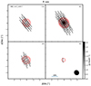 |
Fig. A.1. Same as Fig. 2 but for the SiO v = 1, J = 8 − 7 maser emission around R Leo. The peak emission is ISiOv1, peak = 12.86 Jy beam−1. The maximum polarisation is Pl, max = 32.4%. |
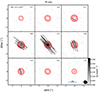 |
Fig. A.2. Same as Fig. 2 but for the SiO v = 2, J = 8 − 7 emission (which likely includes maser amplification) around R Leo. The peak emission is ISiOv1, peak = 0.72 Jy beam−1. The maximum polarisation is Pl, max = 4.92%. |
Appendix B: Polarisation signature of a toroidal magnetic field
In Fig. B.1, we present the model for the CO polarisation in the circumstellar envelope of CW Leo when assuming a purely toroidal magnetic field configuration at the same position angle and inclination as the dipole field model. We note that a purely toroidal field is likely non-physical in a circumstellar envelope, but the model represents the theoretical extreme of a magnetic field with a dominant toroidal component.
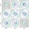 |
Fig. B.1. Same as Fig. 14 but for a range of velocity channels of CO emission emerging from a CSE representative of CW Leo. Here, the symmetry axis of the molecules was chosen to be along the magnetic field, which is assumed as a toroidal field with position angle = 125° and inclination 45°. The simulated data has been convolved with the synthesised beam from the observations. The panels are labelled with the velocity with respect to the stellar velocity. |
All Tables
All Figures
|
Fig. 1. Polarised continuum emission (greyscale) and the 338 GHz continuum contours of CW Leo (left) and R Leo (right). The polarisation peaks at 6.9 and 0.4 mJy beam−1 for CW Leo and R Leo, respectively. The contours are drawn at 0.625%, 1.25%, 2.5%, 5%, 10%, 20%, 40%, and 80% of the peak emission (1.059 and 0.302 Jy beam−1 for CW Leo and R Leo, respectively). The line segments indicate the linear polarisation direction where polarised emission is detected at > 5σP. The uncertainty on the direction is ≲6°. The segments are scaled as indicated by the horizontal bar. The filled ellipses indicate the beam size of the observations. |
| In the text | |
|
Fig. 2. Channel maps of the polarised CO J = 3 − 2 emission around the AGB star CW Leo. The solid red contours indicate the Stokes I total intensity emission at 5%, 10%, 20%, 40%, and 80% of the peak emission (ICO, peak = 17.89 Jy beam−1). The greyscale image is the linearly polarised emission, and the line segments denote the linear polarisation direction where emission is detected at > 5σP. The segments are scaled to the level of fractional polarisation, with the scale indicated in the bottom-right panel. The maximum polarisation is Pl, max = 1.18%. The beam size is denoted in the bottom-right panel, and all panels are labelled with the Vlsr velocity in kilometers per second. The stellar velocity is Vlsr, * = −26.5 km s−1. The dashed blue circles centred on the peak of the CO emission close to the stellar velocity indicates the radius (R ≈ 1.4″) at which we find that the direction of polarisation for CS changes from being neither tangential nor radial to predominantly tangential. |
| In the text | |
|
Fig. 3. Same as Fig. 2 but for the CS J = 7 − 6 emission around CW Leo. The peak emission is ICS, peak = 18.77 Jy beam−1. The maximum polarisation is Pl, max = 1.74%. |
| In the text | |
|
Fig. 4. Same as Fig. 2 but for the H13CN J = 4 − 3 emission around CW Leo. The peak emission is IHCN, peak = 38.52 Jy beam−1. The maximum polarisation is Pl, max = 1.62%. |
| In the text | |
|
Fig. 5. Same as Fig. 2 for the SiS J = 19 − 18 emission around CW Leo. The peak emission is ISiS, peak = 21.01 Jy beam−1. The maximum polarisation is Pl, max = 1.47%. |
| In the text | |
|
Fig. 6. Distribution of polarisation angles with respect to the tangential direction for the emission of CO J = 3 − 2, SiS J = 19 − 18, H13CN J = 4 − 3, and CS J = 7 − 6 around CW Leo. Left: polarisation angles taken from the entire circumstellar envelope emission. Right: polarisation angles for R < 1.4″. |
| In the text | |
|
Fig. 7. Azimuthally averaged Stokes I (top), polarised intensity (Pl; middle), and polarisation fraction (Pl, frac; bottom), taken in the channel that includes the stellar velocity, for CW Leo (left column) and R Leo (right column). For CW Leo, we show CO J = 3 − 2, SiS J = 19 − 18, H13CN J = 4 − 3, and CS J = 7 − 6. For R Leo, we show CO J = 3 − 2, 29SiO v = 0, J = 4 − 3, and H13CN J = 4 − 3. We did not include the mostly unresolved SiO v = 1 and v = 2, J = 8 − 7 transitions. The profiles of Pl and Pl, frac include the error bars from the azimuthal averaging, and only radial points for which the S/N is greater than five are plotted. Because of the averaging, the polarisation fraction is much less than the maximum fraction detected in the image cubes for each line. Beyond one-third, the ALMA primary beam size (at R ≈ 3.0) systematic errors might start to contribute to the polarisation signal. We note that the units for the polarised intensity are different for the two middle plots for CW Leo (Jy beam−1) and R Leo (mJy beam−1). |
| In the text | |
|
Fig. 8. Same as Fig. 2 but for the CO J = 3 − 2 emission around R Leo. The stellar velocity is Vlsr, * = −0.5 km s−1. The peak emission is ICO, peak = 4.66 Jy beam−1. The maximum polarisation is Pl, max = 3.90%. |
| In the text | |
|
Fig. 9. Same as Fig. 2 but for the 29SiO v = 0, J = 8 − 7 emission around R Leo. The peak emission is I29SiO, peak = 8.49 Jy beam−1. The maximum polarisation is Pl, max = 1.57%. |
| In the text | |
|
Fig. 10. Same as Fig. 2 but for the H13CN J = 4 − 3 emission around R Leo. The peak emission is IHCN, peak = 2.40 Jy beam−1. The maximum polarisation is Pl, max = 1.79%. |
| In the text | |
|
Fig. 11. Distribution of polarisation angles with respect to the tangential direction for the emission of CO J = 3 − 2, 29SiO v = 0, J = 8 − 7, and H13CN J = 4 − 3 around R Leo. |
| In the text | |
|
Fig. 12. Comparison of the radiative interaction (solid lines) and magnetic precession rates (dash-dotted lines) of the investigated molecules toward CW Leo. The magnetic precession rates are given for magnetic fields B = Bsurf(R/Rstar)−q, adopting q = 1, q = 2 and 3, where for q = 1 a Bsurf = 1 mG was adopted, while for q = 2 and 3, Bsurf = 1 G was adopted. The black curve composed of long dashes indicates the expected magnetic precession rates that explain the polarisation morphology of CS, CO, and H13CN within 1.4″. The horizontal black dotted and dash-dotted lines indicate the molecular magnetic precession rates at 1 mG and 1 μG, respectively. The vertical black and red dotted lines indicate telescope resolution and the 1.4″ radius where a polarisation morphology change was observed (see Sect. 3.2). The orange coloured region indicates the magnetic field strengths where CO would be aligned to the magnetic field but H13CN would be aligned in the radial direction along the stellar radiation field. |
| In the text | |
|
Fig. 13. Predicted polarised intensity contours (labelled in units of mJy beam−1) overlaid with line segments that indicate the polarisation of (a) H13CN, (b) CS, and (c) SiS emission emerging from a CSE representative of CW Leo. The polarised intensity is given at the systemic velocity channel. The symmetry axis of the molecules was chosen in the radial direction, representative of radiative alignment. The simulated data has been convolved with the synthesised beam from the observations. The panels correspond to the emission in a velocity channel centred on the stellar velocity. |
| In the text | |
|
Fig. 14. Same as Fig. 13 but for a range of velocity channels of CO emission emerging from a CSE representative of CW Leo. The symmetry axis of the molecules was chosen to be along the magnetic field, which we assumed to be a dipole field with a position angle of 125° and inclination of 45°. For this figure, the line segments are scaled according to the polarisation fraction. |
| In the text | |
|
Fig. 15. Comparison of the radiative interaction (solid lines) and magnetic precession rates (dash-dotted lines) of the investigated molecules towards R Leo. Magnetic precession rates are given for magnetic fields B = Bsurf(R/Rstar)−q, adopting q = 2 and 3. The black dotted and dash-dotted lines indicate the molecular magnetic precession rates at 1 mG and 1 μG, respectively. |
| In the text | |
|
Fig. 16. Same as Fig. 13 but for the (a) CO, (b) H13CN, and (c) 29SiO emission emerging from a CSE representative of R Leo. The polarised intensity is given at the systemic velocity channel. The symmetry axis of the molecules was chosen in the radial direction. |
| In the text | |
|
Fig. 17. Dispersion of the polarisation vectors (the square root of the second-order structure function), binned to the Nyquist-sampled resolution, for the central velocity channel of the CO J = 3 − 2 polarised emission around CW Leo. The error bars indicate the variance in each bin. The vertical dotted line indicates the size of the beam’s major axis. The solid line indicates the fit of the structure-function analysis described in the text. |
| In the text | |
|
Fig. 18. Magnetic field strength in AGB circumstellar envelopes as a function of radial distance. The black boxes indicate the literature values reported from maser measurements (e.g. Herpin et al. 2006; Leal-Ferreira et al. 2013; Vlemmings et al. 2005; Rudnitski et al. 2010). The black star indicates the surface magnetic field measurement for the star χ Cyg (Lèbre et al. 2014). The measurements for CW Leo are indicated in red. These are the CN Zeeman measurements from Duthu et al. (2017, red dash-dotted box) and the CO structure-function analysis result reported in Sect. 5.3 (red dashed-dotted line). For the CO result, we used the relation between nH2 and R for the range of radii probed by the ALMA observations (Eq. (6)). This range is indicated by the vertical dotted lines. The stellar surface is indicated by the long-dashed vertical line. For the region probed by ALMA around CW Leo, we indicate in orange the lower (dashed) and upper (solid) magnetic field limits based on the analysis of the 12CO and H13CN radiative interaction rates. The relation between radius and magnetic field strength that fits the observations and modelled radiative rates described in Sect. 4.2 is presented as the blue dashed relation (we extrapolated out to the maximum scale probed with the ALMA polarisation observations). It is clear that this relation is not in agreement with the other magnetic field strength observations. |
| In the text | |
|
Fig. A.1. Same as Fig. 2 but for the SiO v = 1, J = 8 − 7 maser emission around R Leo. The peak emission is ISiOv1, peak = 12.86 Jy beam−1. The maximum polarisation is Pl, max = 32.4%. |
| In the text | |
|
Fig. A.2. Same as Fig. 2 but for the SiO v = 2, J = 8 − 7 emission (which likely includes maser amplification) around R Leo. The peak emission is ISiOv1, peak = 0.72 Jy beam−1. The maximum polarisation is Pl, max = 4.92%. |
| In the text | |
|
Fig. B.1. Same as Fig. 14 but for a range of velocity channels of CO emission emerging from a CSE representative of CW Leo. Here, the symmetry axis of the molecules was chosen to be along the magnetic field, which is assumed as a toroidal field with position angle = 125° and inclination 45°. The simulated data has been convolved with the synthesised beam from the observations. The panels are labelled with the velocity with respect to the stellar velocity. |
| In the text | |
Current usage metrics show cumulative count of Article Views (full-text article views including HTML views, PDF and ePub downloads, according to the available data) and Abstracts Views on Vision4Press platform.
Data correspond to usage on the plateform after 2015. The current usage metrics is available 48-96 hours after online publication and is updated daily on week days.
Initial download of the metrics may take a while.