| Issue |
A&A
Volume 671, March 2023
|
|
|---|---|---|
| Article Number | A117 | |
| Number of page(s) | 11 | |
| Section | Stellar structure and evolution | |
| DOI | https://doi.org/10.1051/0004-6361/202244912 | |
| Published online | 13 March 2023 | |
Polarisation of molecular lines in the circumstellar envelope of the post-asymptotic giant branch star OH 17.7–2.0
Department of Space, Earth and Environment, Chalmers University of Technology, Onsala Space Observatory, 439 92 Onsala, Sweden
e-mail: This email address is being protected from spambots. You need JavaScript enabled to view it.
Received:
7
September
2022
Accepted:
30
January
2023
Abstract
Context. The role of magnetic field in shaping planetary nebulae (PNe), either directly or indirectly after being enhanced by binary interaction, has long been a topic of debate. Large-scale magnetic fields around pre-PNe have been inferred from polarisation observations of masers. However, because masers probe very specific regions, it is still unclear if the maser results are representative of the intrinsic magnetic field in the circumstellar envelope (CSE).
Aims. Molecular line polarisation of non-maser lines can provide important information about the magnetic field. A comparison between the magnetic field morphology determined from maser observations and that observed in the more diffuse CO gas can reveal if the two tracers probe the same magnetic field.
Methods. We compared observations taken with the Atacama Large Millimeter/submillimeter Array (ALMA) of molecular line polarisation around the post-asymptotic giant branch (post-AGB) or pre-PN star OH 17.7−2.0 with previous observations of polarisation in the 1612 MHz OH maser region. Earlier mid-infrared observations indicate that OH 17.7−2.0 is a young bipolar pre-PN, with both a torus and bipolar outflow cavities embedded in a remnant AGB envelope.
Results. We detect CO J = 2 − 1 molecular line polarisation at a level of ∼4% that displays an ordered linear polarisation structure. We find that, correcting for Faraday rotation of the OH maser linear polarisation vectors, the OH and CO linearly polarised emission trace the same large-scale magnetic field. A structure function analysis of the CO linear polarisation reveals a plane-of-the-sky magnetic field strength of B⊥ ∼ 1 mG in the CO region, consistent with previous OH Zeeman observations.
Conclusions. The consistency of the ALMA CO molecular line polarisation observation with maser observations indicate that both can be used to determine the magnetic field strength and morphology in CSEs. The new observations indicate that the magnetic field has a strong toroidal field component projected on the torus structure and a poloidal field component along the outflow cavity. The existence of a strong, ordered, magnetic-field around OH 17.7−2.0 indicates that the magnetic field is likely involved in the formation of this bipolar pre-PN.
Key words: stars: AGB and post-AGB / circumstellar matter / magnetic fields / stars: individual: OH 17.7−2.0
© The Authors 2023
 Open Access article, published by EDP Sciences, under the terms of the Creative Commons Attribution License (https://creativecommons.org/licenses/by/4.0), which permits unrestricted use, distribution, and reproduction in any medium, provided the original work is properly cited.
This article is published in open access under the Subscribe to Open model. This email address is being protected from spambots. You need JavaScript enabled to view it. to support open access publication.
1. Introduction
The processes involved in the formation of bipolar planetary nebulae (PNe) are still under debate (e.g. Blackman 2022). While there are strong indications that binary interaction is required (e.g. Boffin & Jones 2019, and references therein), there are also observations that show that magnetic fields appear responsible for launching collimated outflows that shape the nebula (e.g. Vlemmings et al. 2006). It is possible that binarity and magnetic fields work in tandem. In this case, the magnetic field is enhanced by the interaction between the evolved star, typically during the red-giant branch (RGB) or asymptotic-giant branch (AGB) phase of their evolution, and a companion (e.g. Nordhaus & Blackman 2006). This interaction could lead to a common-envelope evolution (CEE), where the tenuous envelope of the RGB/AGB star is ejected while accretion on the companion or evolved star core, assisted by enhanced magnetic fields, launches a bipolar outflow (e.g. Ondratschek et al. 2022). Observations of a large sample of evolved stars with fast bipolar outflows indicate that these bipolar pre-PNe likely make up the majority of the recent CEE ejection events (Khouri et al. 2021).
Strong magnetic fields have also been observed around early-AGB stars and post-AGB (pre-PN) objects that have no confirmed companion or that have not yet undergone a CEE event (e.g. Vlemmings 2019, and references therein). The origin of these fields is still unclear. The majority of the magnetic field observations around evolved stars have relied on measurements of linear and circular polarisation of masers due to the Zeeman-effect (e.g. Vlemmings et al. 2002, 2005, 2006; Bains et al. 2003; Herpin et al. 2006; Leal-Ferreira et al. 2013; Gonidakis et al. 2014). Additionally, there are observations of the surface magnetic field on one AGB star (Lèbre et al. 2014), as well as on the surface of two post-AGB stars (Sabin et al. 2015). Observations of polarised dust (e.g. Sabin et al. 2020) and radio synchrotron emission (Perez-Sanchez et al. 2013) around post-AGB stars might also indicate the involvement of magnetic fields in shaping PNe. Still, to date, the strongest evidence of the role of magnetic fields specifically around post-AGB objects comes from maser observations (e.g. Bains et al. 2003; Vlemmings et al. 2006) that provide both a magnetic field morphology and magnetic field strength. It has, however, been argued that the magnetic fields determined from maser observations are biased due to the special nature of the amplified stimulated emission that produces maser features in very specific region in the CSE (e.g. Soker 2002).
Molecular line polarisation from non-maser molecules, resulting from the Goldreich-Kylafis (GK) effect (e.g. Goldreich & Kylafis 1982; Lankhaar & Vlemmings 2020), can be used to determine if the maser magnetic field observations probe the intrinsic large-scale magnetic field. The GK effect of CO and other molecules has been observed in star forming regions, proto-planetary discs, and around a supergiant star (e.g. Li & Henning 2011; Cortés et al. 2005, 2021; Beuther et al. 2010; Vlemmings et al. 2017; Stephens et al. 2020; Teague et al. 2021). It has also been detected, using the Submillimeter Array (SMA), around the AGB stars CW Leo and IK Tau (Girart et al. 2012; Vlemmings et al. 2012) and with the Combined Array for Research in Millimeter-wave Astronomy (CARMA) towards R Leo and R Crt (Huang et al. 2020). While these observations indicated a possible large-scale magnetic field, the sensitivity of the SMA and CARMA was not sufficient for the detection of polarised molecular line emission in more than a few compact regions of the CSE. For most of the previously observed sources, no maser polarisation observations probing the same region as probed by the GK-effect exist. It has thus not been possible to compare the observations directly with maser measurements.
One of the post-AGB sources with extensive polarised OH maser observations is the pre-PN star OH 17.7−2.0. Polarisation observations mainly of the 1612 MHz OH masers around this source revealed an apparent coherent large scale structure with a magnetic field strength in the OH maser region of B ≈ 2.5 − 4.5 mG (Bains et al. 2003, herafter B03). Here, we present ALMA observations of linear polarisation due to the GK effect in the envelope of OH 17.7−2.0. In Sect. 2, we present the observations and data reduction, and in Sect. 3 we present the source, with a particular discussion regarding its distance. In Sect. 4, we present the results of the ALMA observations, and in Sect. 5 we describe a structure function analysis (SFA) we used to estimate the magnetic field strength, perform a detailed comparison with the OH maser observation of B03, and present our results on the morphology of the magnetic field around OH 17.7−2.0. We end with our conclusions in Sect. 6.
2. Observations and data reduction
The CSE of OH 17.7−2.0 was observed by ALMA in full polarisation mode on April 14 2018 over a total time of 2.5 h. The on-source time was ∼70 min. The remaining time was spent observing the phase calibrator J1832+2039 and the amplitude and polarisation calibrator J1924+2914. Four spectral windows of 1.875 GHz and 960 channels were centred on 214.6, 216.5, 228.6, and 230.5 GHz, resulting in a channel width of ∼2.6 km s−1. The observations were calibrated using the ALMA polarisation calibration scripts (Nagai et al. 2016).
Subsequent calibration, self-calibration and imaging was done using CASA 5.7.2 (McMullin et al. 2007)1. We performed two rounds of phase-only self-calibration on the compact continuum of OH 17.7−2.0, which improved the dynamic range in the continuum from ∼530 to ∼1010. The observations reach a continuum rms in Stokes I (σI) of 71 μJy beam−1. In the Stokes Q and U continuum images, the rms noise (σQ, U) is ∼13 μJy beam−1 and ∼18 μJy beam−1, respectively. We also produced the Stokes V continuum image, for which we find an rms noise σV of ∼14 μJy beam−1. While the rms in the Stokes Q, U, and V images are close to the theoretical noise limit, that of Stokes I is almost five times higher. The continuum Stokes I image is thus likely limited by dynamic range. The continuum beam size, using Briggs weighing and a robust parameter of 0.5, is 0.78 × 0.65″ (PA 75.1°).
The continuum was subtracted using the CASA task uvcontsub, and the strongest spectral lines were subsequently imaged using Briggs weighing and a robust parameter of 0.5. To improve polarisation sensitivity, we averaged two channels, obtaining a velocity resolution of ∼5.2 km s−1. The σI, σQ, σU, and σV rms noise levels in a line free channel are 0.64 mJy beam−1, 0.39 mJy beam−1, 0.38 mJy beam−1, and 0.47 mJy beam−1. The beam size at 230 GHz is 0.77 × 0.64″ (PA 77.3°). The maximum recoverable scale in our observations is ∼8.1″. From a comparison with the published CO J = 2 − 1 spectrum (Heske et al. 1990) and a visual inspection of the images, there are no indications of significant resolved out flux. Finally, linear polarisation maps were created from the Stokes Q and U images using  . The polarisation rms σP ≈ 0.5 mJy beam−1 is found from an analysis of the rms in a line free spectral channel for each spectral line individually.
3. OH 17.7–2.0
The pre-PN star OH 17.7−2.0, also known as IRAS 18276−1431, has been studied across a wide range of wavelengths. It hosts strong OH masers (e.g. Bowers 1978), while its H2O masers disappeared after a rapid flux decline between 1985 and 1990 (Engels 2002) before reappearing more than 20 years later (Wolak et al. 2013). The decrease of H2O maser emission was attributed to a recent drop in mass-loss rate caused by the star having recently left the AGB phase. Polarimetric measurements of OH masers appear to indicate that the CSE of OH 17.7−2.0 has a strong large-scale magnetic field (B03). OH 17.7−2.0 was first suggested be a bipolar nebula based on an analysis of its infrared (IR) spectral energy distribution (Le Bertre et al. 1984). Later imaging in the optical and (near-)IR confirmed this view (e.g. Sánchez Contreras et al. 2007; Gledhill et al. 2011; Lagadec et al. 2011; Murakawa et al. 2013). Observations of H2 and CO emission in the near-IR suggest a bipolar outflow velocity of ∼95 km s−1. The outflow has created bipolar outflow cavities that are ≳-pagination125 yr old and are inclined towards the line-of-sight by ∼22° (Gledhill et al. 2011). Observations of the 12CO and 13CO J = 1 − 0 emission using the Owens Valley Radio Observatory (OVRO) revealed that the source is embedded in a dense, mostly spherical, CO envelope that has an outflow velocity of ∼17 km s−1 (Sánchez Contreras et al. 2007; Sánchez Contreras & Sahai 2012). No fast outflow is detected in the sub-millimetre CO emission. In Murakawa et al. (2013), a model was created to match the near-IR spectral energy distribution and polarised emission. They conclude, assuming a distance of 3 kpc, that most of the dust resides in a torus with inner and outer radii of 30 and 1000 au. The torus has a total mass of 3.0 M⊙ and, assuming an expansion of the torus with a velocity similar to the velocities measured in the CO J = 1 − 0, an age of ∼300 yr.
With regard to the distance to OH 17.7−2.0, because foreground Faraday rotation of the linearly polarised OH maser emission affects the comparison of the absolute polarisation angle between the OH and sub-millimetre molecular line emission, we carefully assessed the distance to OH 17.7−2.0. In the literature, distances are quoted from ∼2 − 5.4 kpc. Some of the earliest distances were derived using the phase-lag method, comparing the size of the OH maser shell with the delay between the infrared and OH maser variability curve. This yielded distances ranging from 3.4 − 5.4 kpc using measurements from Bowers et al. (1983), or 2 − 5.5 kpc, using those from Herman & Habing (1985). Alternatively, the (near) kinematic distance, for a source velocity VLSR, * = 62 km s−1, gives a distance of  kpc (Reid et al. 2014). Finally, the luminosity distance, assuming a source luminosity of 6000 L⊙, is 2.94 ± 0.38 kpc (Vickers et al. 2015). In Gaia Data Release 3 (Gaia DR3, Gaia Collaboration 2021), four sources are identified within 2.5″ of the position of the sub-millimetre continuum peak found in our ALMA observations. The Gaia source identification number, offsets, and Gaia parallax results are shown in Table 1, and the positions are noted in Fig. 1. It is clear that the two first Gaia sources are not related to OH 17.7−2.0. In fact, their positions coincide exactly with the field sources seen in the near-infrared observations of Sánchez Contreras et al. (2007) and Gledhill et al. (2011). The two remaining Gaia sources correspond exactly with the scattered light emission coming from the two outflow lobes of OH 17.7−2.0 seen in the same observations. However, unsurprisingly, no reliable astrometry could be performed on these two lobes. Based on these results, we adopt the luminosity distance from Vickers et al. (2015) of D = 2.94 ± 0.38 kpc as the most reliable at the moment.
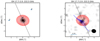 |
Fig. 1. 222.5 GHz continuum emission from OH 17.7−2.0 in red contours. The contours are drawn at 0.625, 1.25, 2.5, 5, 10, 20, 40, and 80% of the peak value of 71.8 mJy beam−1. The dashed line indicates the direction of the outflow inferred from mid-infrared continuum and H2 observations (Gledhill et al. 2011). Left: the four labelled solid circles are the sources identified by Gaia within a radius of 2.5″ of OH 17.7−2.0 (see text). The greyscale also represents the continuum emission. Right: the polarised continuum emission (greyscale) of OH 17.7−2.0. The blue line segments indicate the linear polarisation direction where polarised emission is detected at > 3σ, where the rms on the polarised emission σ = 21 μJy beam−1. This means that the uncertainty on the direction is ≲10°. The segments are scaled by the linear polarisation fraction which peaks at Pl, max = 0.47%. The filled ellipse indicates the beam size of the observations. |
Gaia results.
4. Observational results
We detected significant (> 3σ) polarised emission towards the 222.5 GHz continuum of OH 17.7−2.0. The maximum fraction of continuum polarisation is 0.47%. This is a lower fraction than the continuum polarisation detected with ALMA towards the post-AGB object OH 231.8+4.2 (Sabin et al. 2020) (at ∼345 GHz). We detect no circular polarisation signal in the Stokes V continuum image, so can place a 3σ limit on the continuum circular polarisation of 0.58%.
Molecular line linear polarisation is detected (at > 5σ) for four of the five strongest molecular transitions detected in our observations. The five transitions, all detected with a peak emission of > 0.1 Jy beam−1, are presented with their peak fluxes and maximum linear polarisation fraction (and 5σ polarisation upper limit towards the peak of the line emission, in cases of non-detection) in Table 2. Channel maps of the four lines for which polarisation was detected, CO J = 2 − 1, 29SiO J = 5 − 4, SiO J = 5 − 4, and SO J = 5 − 4, are shown in Figs. 2, A.1–A.3, respectively. In addition to the linear polarisation, we also investigated the circular polarisation we detected for any of the molecular lines. Compact, negative, Stokes V emission was detected in four channels towards the peak of the Stokes I emission of CO J = 2 − 1. The (absolute) maximum fractional circular polarisation Pv, max = 0.41%. The other lines did not display significant Stokes V emission. Currently, the minimum detectable degree of circular polarisation, defined as three times the systematic calibration uncertainty, is 1.8%2, compared to 0.1% for linear polarisation. As the measured level of the CO circular polarisation is below this, the circular polarisation is likely a result of the systematic calibration uncertainties. Still, we briefly discuss the measurement in Sect. 5.2 in relation to possible contributions from anisotropic resonance scattering (Houde et al. 2013, 2022).
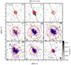 |
Fig. 2. Channel maps of polarised CO J = 2 − 1 emission around the post-AGB star OH 17.7−2.0. The Stokes I total intensity emission is indicated by the solid red contours at 2.5, 5, 10, 20, 40, and 80% of the peak emission (ICO, peak = 1.04 Jy beam−1). The linearly polarised emission is shown as a greyscale map, and the blue line segments denote the linear polarisation direction when the polarised emission > 5σP. The uncertainty on the polarisation direction is thus ≲7°. The segments are scaled to the level of fractional polarisation with the scale indicated in the bottom left panel. The maximum polarisation Pl, max = 4.1%. The panels are labelled with the VLSR velocity in km s−1, and the beam size is shown in the bottom right panel. The stellar velocity VLSR, * = 62.0 km s−1. The dashed line indicates the direction of the outflow of OH 17.7−2.0, as in Fig. 1. |
OH 17.7−2.0 line polarisation.
Only for the CO J = 2 − 1 do we detect significant polarisation across several consecutive velocity channels and in extended regions of more than 3″ in size. The polarisation direction for the CO appears to curve from an angle of ∼120° towards the south along the outflow axis, to ∼35° towards the north. This means it goes from being nearly perpendicular to the outflow to being nearly parallel to the outflow. In contrast, the 29SiO v = 0, J = 5 − 4 has, at blue-shifted velocities, polarisation vectors that lie at and angle of approximately 45° with respect to the outflow axis. Around VLSR = 68.5 km s−1, the detected polarisation is perpendicular to the outflow. Polarisation of SiO v = 0, J = 5 − 4 is only detected in one area, at VLSR = 68.3 km s−1; this is towards the north on the outflow axis, where the polarisation is perpendicular to the outflow. Finally, the SO J = 5 − 4 also only displays one region of significant polarisation, at VLSR = 56.1 km s−1, with a direction similar to that of the CO at the same velocity.
5. Discussion
5.1. Continuum polarisation
As seen in Fig. 1 (right), the continuum polarisation is confined to a small area slightly offset from the continuum peak. While the central star contributes to the emission, the largest contribution comes from the circumstellar dust. Considering our spatial resolution is not sufficient to resolve details in the continuum emission, and there are no observations at other frequencies that can be used to constrain the dust properties or the alignment mechanism, we do not provide an in-depth analysis of the dust polarisation. As shown in Vlemmings et al. (2017) for the supergiant VY CMa, for example, the dust polarisation is likely due to alignment of the dust particles with the magnetic field. In Fig. 3, we compare the continuum polarisation direction with those of the CO J = 2 − 1 emission in spectral channels close to the systemic velocity. As seen in the comparison, the direction of the polarisation is completely consistent within the polarisation direction uncertainties, indicating that the origin of the polarisation in the molecular lines and continuum is related.
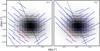 |
Fig. 3. Zoomed-in view of continuum emission (grey scale) of OH 17.7−2.0 with the blue line segments denoting the linear polarisation of CO J = 2 − 1 for the two channels around the systemic velocity (labelled in km s−1 in the top right corner). The dashed red line segments indicate the linear polarisation direction of the continuum polarisation. The black dashed line indicates the direction of the bipolar outflow. |
5.2. Anisotropic resonant scattering
Anisotropic resonant scattering can affect the polarisation properties of molecular line emission when it passes through a magnetised molecular region in the foreground between the source and the telescope (Houde et al. 2013, 2022). It can also occur in the emitting molecular line region itself. This process results in a transformation from linear to circular polarisation. Consequently, the linear polarisation direction is potentially no longer directly related to the magnetic field direction.
Since the emitting CO region around evolved stars is limited by CO photo-dissociation in the outer CSE, there is unlikely to be a large column of CO molecules in the foreground towards the source. Additionally, the large velocity gradient in an expanding CSE, towards all but the extreme velocities, further reduces the foreground column of gas at the emitting velocity towards most lines of sight. Thus, anisotropic resonance scattering of the polarised CO line emission from CSEs is likely limited to the scattering that occurs in the emitting region itself.
If anisotropic resonance scattering affects the linearly polarised emission detected in our observations, we expect a component of circular polarisation in the affected regions. Although, as described in Sect. 2, the level of circular polarisation observed for the CO J = 2 − 1 emission is below the level that is considered significant in light of ALMA systematic circular polarisation calibration errors, we still compare the detected circular polarisation of ∼0.4% to the observed linear polarisation. As can be seen in Fig. 4, the circular polarisation is confined to the central part of the emission, with a size of approximately one interferometric beam. The linear polarisation vectors trace a smooth curved pattern through the region where there is a potential detection of circular polarisation. In the same region where the circular polarisation occurs, the direction of the continuum and CO linear polarisation is consistent (Fig. 3), which implies that there is no extra rotation of the polarisation vectors. We conclude that anisotropic resonant scattering does not affect our measurements.
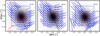 |
Fig. 4. Zoomed-in view of central region of CO J = 2 − 1 emission previously shown in Fig. 2. The greyscale indicates the Stokes I emission and the blue line segments indicate the linearly polarisation direction. The red dashed contours represent the (negative) Stokes V emission at −8, −6, and −4σ, where σ = 0.4 mJy beam−1. The outflow direction is indicated by the dashed line. The blue box indicates the region of the 1612 MHz OH masers for which a linear polarisation map is presented in B03 (their Fig. 7). The majority of the OH masers are located within ∼0.4″ of the centre of the map. The channel velocity in km s−1 is given the top right corner of each panel. |
5.3. Magnetic field strength: Structure function analysis
Similarly to what is often done in studies of magnetic fields during star formation (e.g. Hildebrand et al. 2009; Koch et al. 2010; Houde et al. 2016; Dall’Olio et al. 2019) we used the CO polarisation observations to provide an estimate of the magnetic field strength through a structure function analysis (SFA). The SFA analysis relates the dispersion of polarisation vectors at the smallest scales to the turbulent motions in the magnetised gas to provide the ratio between the turbulent and mean large scale magnetic field strength. The SFA can thus be used to characterise turbulence. Under the assumption that the magnetic field is frozen into the gas, that the turbulent field arises from transverse Alfvén waves, and that the turbulence is isotropic and incompressible, the ratio between the turbulent and mean large-scale magnetic field strength determined using a SFA analysis can also be used to estimate the magnetic field strength.
In the following, we repeat the equations for the SFA from Koch et al. (2010). In the SFA, the dispersion of polarisation vectors is determined using the following equation:
 (1)
(1)
where χ(ri) is the polarisation angle at the position ri = (xi, yi),  , lk indicates the binning interval of the scale (taken in arcseconds), and N(lk) are the numbers of points averaged in each bin. It was shown in Hildebrand et al. (2009) that for a smooth magnetic field component B0 and a small-scale turbulent magnetic field component Bt, the structure function, on scales between the smallest turbulent scale and the characteristic length scale for variations in the large scale component, can be described with:
 (2)
(2)
Here, m is the slope of the linear dispersion term of the large scale field B0 and σM(lk) propagates the observational uncertainties on the polarisation vectors in the binning. The term b is then related to the ratio between the turbulent and large scale magnetic field strengths through
 (3)
(3)
Under the assumptions introduced previously, the ratio between the turbulent and large-scale magnetic field component is equal to the ratio between the turbulent line width σν and the Alfvén velocity  , with ρ the density of the gas. Using the turbulent velocity and average density in the CO emitting region allows us to determine the magnetic field strength in the plane of the sky. This strength will be a lower limit in the case the magnetic field is not fully frozen into the gas.
The result of the SFA for two spectral channels, with the CO gas at VLSR = 57.3 km s−1 and 62.4 km s−1 around OH 17.7−2.0 are shown in Fig. 5. As expected, the dispersion of the polarisation vectors increase from a smaller to a larger scale. For the channel close to the stellar velocity, the dispersion subsequently decreases steeply due to the aligned polarised emission at a larger radius towards the northeast. The structure function is fitted using Eq. (3) within ≲2.3″ (three synthesised beams), which we take to correspond to a characteristic length scale for variations in the large-scale magnetic field component. We note that for both velocity channels, the polarisation vector dispersion at the smallest scales available in our observations is ∼20°. The analysis provides a ratio between the turbulent and large scale magnetic field component  , and 0.14 ± 0.01 for the two channels, respectively. This means that the large-scale magnetic field strength for both channels is
![Mathematical equation: $$ \begin{aligned} B_0 = [2.3, 1.6] \left(\frac{\langle n_{\rm H_2}\rangle }{10^5}\right)^{1/2} \frac{v_{\rm t}}{1.0}\,\mathrm{mG}. \end{aligned} $$](/articles/aa/full_html/2023/03/aa44912-22/aa44912-22-eq9.gif) (4)
(4)
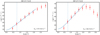 |
Fig. 5. Dispersion of polarisation vectors (the square root of the second-order structure function) binned to the Nyquist sampled resolution, for two velocity channels of the CO J = 2 − 1 polarised emission around OH 17.7−2.0. The error bars indicate the variance in each bin. The vertical dotted line indicates the size of the beam major axis. The solid line indicates the fit of the structure function analysis described in the text. |
Here, vt is the turbulent velocity in the CO gas, taken to be 1.0 km s−1 derived from CO radiative transfer modelling of AGB envelopes (e.g. Vlemmings et al. 2021). From similar models, the average H2 number density nH2 in the CO region is assumed to be 105 cm−3. These assumptions, as well as the assumption that the magnetic field is frozen into the gas, dominate the uncertainty in the magnetic field strength. Similar results are obtained for the other channels for which a SFA could be performed. The polarised emission of the other molecular lines is limited to compact regions not much larger than our interferometric beam, and hence a SFA was not possible.
Houde et al. (2016) showed that a combination of the resolution of the observations and interferometric spatial filtering affect the results from the SFA. In Sect. 2 we show that the maximum recoverable scale of our observations (∼8.1″) is sufficiently large that spatial filtering does not affect our analysis. In order to determine the effect of the beam size, we estimate the number of independent turbulent cells (N) probed by our observations using the formula from Houde et al. (2016):
 (5)
(5)
Here, δ is the correlation length of the turbulent field, W1 is the radius of the interferometric beam (we use  times an average FWHM beam size of 0.72″) and Δ′ is the depth of the observed molecular layer along the line of sight. For a source at D = 2.94 kpc, our beam radius is W1 ∼ 900 au. We estimated the depth Δ′ from the total size of the CO envelope (∼18 000 au) divided by the number of channels, yielding Δ′∼1800 au (although, considering the spherically expanding CSE, this value actually varies across the envelope). Finally, we estimate the correlation length δ to be similar to the size of the molecular clumps that make up the envelope. Richards et al. (2012) derived, from H2O maser measurements, that these clumps start out with a size of the order of the stellar radius and expand for increasing distance to the star. Combined with CO observations and models (e.g. Olofsson et al. 1996), Richards et al. (2012) suggested that the clump size rc appears to scale with the distance from the star r being rc ∝ r0.8. Applying these estimates to the CO J = 2 − 1 gas around OH 17.7−2.0 yields a size of ∼850 au. Hence, taking δ ∼ 850 au, W1 ∼ 900 au, and Δ′∼1800 au we find N ∼ 2.7. As the ratio between the turbulent and large-scale magnetic field strengths scales approximately with
  , our magnetic field estimate would be overestimated by a factor of ∼1.7. Considering the various uncertainties in all the different assumptions, we conclude that the order-of-magnitude strength of the plane-of-sky component of the magnetic field that permeates the CO emitting region is B⊥ ∼ 1 mG.
We can compare these results with the OH maser Zeeman measurements from B03. The Zeeman measurements of the paramagnetic OH molecule provide an estimate of the total magnetic field strength of B = 2.5 − 4.6 mG. Since our measurement estimates the plane of the sky component of the magnetic field, the CO results are fully consistent with the OH Zeeman measurements.
5.4. Comparison with OH linear polarisation results
As previously indicated, a large-scale magnetic field was mapped around OH 17.7−2.0 using OH maser observations (B03). This allows for a direct comparison between the magnetic field traced in individual 1612 MHz OH maser clumps and that in the more diffuse CO gas. The area covered by the OH masers is shown in a zoomed-in image of the three central velocity channels of our CO observations in Fig. 4. First, the maser positions were aligned with the CO observations by assuming that the centre of the maser shell fitted in B03 coincides with the peak of the continuum emission from our observations. Subsequently, each maser spot in Table 4 of B03 was identified with the nearest 0.1″ pixel and nearest velocity channel in our observations. For pixels that contained multiple maser spots, a weighted average OH maser polarisation angle was calculated. Subsequently, the mean angle was subtracted from both the OH polarisation angle (⟨χOH⟩ = 70.7°) and CO polarisation angle (⟨χCO⟩ = 81.6°) distributions. This was done because the OH maser polarisation angle is likely significantly affected by Faraday rotation (see below). The absolute angle difference |Δχ|=|(χOH − ⟨χOH⟩) − (χCO − ⟨χCO⟩)| is shown in Fig. 6.
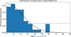 |
Fig. 6. Distribution of absolute angle difference between 1612 MHz OH masers (B03) and CO polarisation direction. The mean difference, which can be affected by Faraday rotation, has been removed (see text). The solid black line indicates a normal distribution, and σ = 22.5°, which corresponds to the best-fit normal distribution. The dashed line represents a uniform distribution of angle differences. |
We find that the angle difference distribution can be best described by a normal distribution with a standard deviation σ = 22.5°. This is similar to the dispersion angle of the CO at the smallest scales as found in the SFA analysis in Sect. 5.3. Hence, considering the similarity between the angle difference distribution and the dispersion in the angle expected to occur in both the OH masing gas and CO gas as a result of turbulence, we can confidently state that the magnetic field traced by the more diffuse CO gas and the OH maser clumps behaves similarly.
5.5. Magnetic field morphology
The OH maser observations of B03 indicated that a large-scale magnetic field is present around OH 17.7−2.0. The OH polarisation was attributed to emission from elliptically polarised σ components that are the result of Zeeman splitting. This means that the polarisation vectors are perpendicular to the magnetic field direction. However, because foreground Faraday rotation is significant at OH maser frequencies, it was not possible to relate the polarisation direction with, for example, the outflow direction or inferred toroidal structure. Because the CO observations correspond to higher frequency emission (∼230 GHz) compared to the OH maser observations at 1612 MHz, foreground Faraday rotation will be significantly less for our CO observations. We can estimate the Faraday rotation by using the best distance estimate (2.94 kpc, see Sect. 3), a typical value for the interstellar magnetic field of 2 μG (Sun et al. 2008) and an average electron number density ne = 0.01066 cm−3 on the line of sight to OH 17.7−2.0 (Yao et al. 2017). For the 1612 MHz OH masers, this implies a Faraday rotation of ΔΦ = 102° while for CO the rotation would be negligible (< 0.005°). Comparing this with the difference in mean angle between the OH and CO polarisation vectors found in Sect. 5.4 of ∼ − 11°; this would imply an intrinsic angle difference of ∼91°. This is remarkably close to perpendicular and strongly implies a relation between the polarisation measured on the masers and in the CO envelope. Considering the OH polarisation is perpendicular to the magnetic field, the CO polarisation is parallel to the magnetic field. Thus, the curvature in the CO polarisation going from being perpendicular to the outflow to being nearly parallel to the outflow implies that we are tracing a dominant toroidal magnetic field component towards the south of the continuum peak and a helical or nearly poloidal field component towards the northern part of the outflow. This is likely the result of the inclination of the outflow, which was estimated to be ∼22° with the blueshifted outflow in the north and the redshifted outflow in the south (Gledhill et al. 2011). Towards the south, we thus mostly probe gas in front of the outflow cavity, while in the north we probe part of the outflow cavity itself. Such a morphology is similar to that of magnetically driven outflow models such as a magnetic tower jet (e.g. Huarte-Espinosa et al. 2012), a configuration that was also inferred for the post-AGB object OH 231.8+4.2 (Sabin et al. 2020). As already noted in B03, the magnetic energy dominates the mechanical energy in the regions probed by the OH masers, and, considering the similar field strength estimated from the CO observations, the same holds true for the gas probed by the CO emission.
6. Conclusions
We have observed molecular line polarisation in the CSE of the post-AGB (or pre-PN) star OH 17.7−2.0 using ALMA. The observations of the polarisation arising from the GK-effect have allowed us to determine the magnetic field strength in the CO-emitting region using an SFA. The strength of the magnetic field component in the plane of the sky was found to be ∼1 mG, which is consistent with previous Zeeman measurements using OH masers (B03). A comparison between the OH maser and CO linear polarisation vectors indicates that, although the OH maser polarisation direction is strongly affected by foreground Faraday rotation, the magnetic field in the OH masers and in the CO gas is likely the same. This confirms that the magnetic field properties, except for the absolute magnetic field direction on the sky, derived from OH masers are representative of the large-scale circumstellar magnetic field. The magnetic field structure derived from the ALMA CO observations is similar to that expected for a magnetically driven outflow. As previously noted from the OH Zeeman observations, the magnetic energy also dominated the energy budget in the envelope. More detailed observations of the outflow launching region around OH 17.7−2.0 are needed to firmly identify the mechanism responsible for the structures seen around this pre-PN star. The observations presented here show that molecular line polarisation observations, of both maser and non-maser species, are invaluable to determine the role of magnetic fields during the late stages of stellar evolution.
The data were checked against an error in visibility amplitude calibration (https://almascience.eso.org/news/amplitude-calibration-issue-affecting-some-alma-data), but ALMA staff from the ESO ALMA Regional Centre determined that a correction was not necessary.
ALMA Cycle 9 Technical handbook.
Acknowledgments
We thank the referee, Martin Houde, for comments that improved the paper. This paper makes use of the following ALMA data: ADS/JAO.ALMA#2016.1.00251.S. ALMA is a partnership of ESO (representing its member states), NSF (USA) and NINS (Japan), together with NRC (Canada), NSC and ASIAA (Taiwan), and KASI (Republic of Korea), in cooperation with the Republic of Chile. The Joint ALMA Observatory is operated by ESO, AUI/NRAO and NAOJ. The project leading to this publication has received support from ORP, that is funded by the European Union’s Horizon 2020 research and innovation programme under grant agreement No. 101004719 [ORP]. We also acknowledge support from the Nordic ALMA Regional Centre (ARC) node based at Onsala Space Observatory. The Nordic ARC node is funded through Swedish Research Council grant No. 2017-00648.
References
- Bains, I., Gledhill, T. M., Yates, J. A., et al. 2003, MNRAS, 338, 287 [NASA ADS] [CrossRef] [Google Scholar]
- Beuther, H., Vlemmings, W. H. T., Rao, R., et al. 2010, ApJ, 724, L113 [NASA ADS] [CrossRef] [Google Scholar]
- Blackman, E. G. 2022, Proc. IAU, 366, 281 [NASA ADS] [Google Scholar]
- Boffin, H. M. J., & Jones, D. 2019, The Importance of Binaries in the Formation and Evolution of Planetary Nebulae (Springer Nature Switzerland AG) [Google Scholar]
- Bowers, P. F. 1978, A&AS, 31, 127 [NASA ADS] [Google Scholar]
- Bowers, P. F., Johnston, K. J., & Spencer, J. H. 1983, ApJ, 274, 733 [NASA ADS] [CrossRef] [Google Scholar]
- Cortés, P. C., Crutcher, R. M., & Watson, W. D. 2005, ApJ, 628, 780 [NASA ADS] [CrossRef] [Google Scholar]
- Cortés, P. C., Sanhueza, P., Houde, M., et al. 2021, ApJ, 923, 204 [CrossRef] [Google Scholar]
- Dall’Olio, D., Vlemmings, W. H. T., Persson, M. V., et al. 2019, A&A, 626, A36 [NASA ADS] [CrossRef] [EDP Sciences] [Google Scholar]
- Engels, D. 2002, A&A, 388, 252 [NASA ADS] [CrossRef] [EDP Sciences] [Google Scholar]
- Gaia Collaboration (Brown, A. G. A., et al.) 2021, A&A, 649, A1 [NASA ADS] [CrossRef] [EDP Sciences] [Google Scholar]
- Girart, J. M., Patel, N., Vlemmings, W. H. T., et al. 2012, ApJ, 751, L20 [NASA ADS] [CrossRef] [Google Scholar]
- Gledhill, T. M., Forde, K. P., Lowe, K. T. E., et al. 2011, MNRAS, 411, 1453 [CrossRef] [Google Scholar]
- Goldreich, P., & Kylafis, N. D. 1982, ApJ, 253, 606 [NASA ADS] [CrossRef] [Google Scholar]
- Gonidakis, I., Chapman, J. M., Deacon, R. M., et al. 2014, MNRAS, 443, 3819 [NASA ADS] [CrossRef] [Google Scholar]
- Herman, J., & Habing, H. J. 1985, A&AS, 59, 523 [NASA ADS] [Google Scholar]
- Herpin, F., Baudry, A., Thum, C., et al. 2006, A&A, 450, 667 [NASA ADS] [CrossRef] [EDP Sciences] [Google Scholar]
- Heske, A., Forveille, T., Omont, A., et al. 1990, A&A, 239, 173 [NASA ADS] [Google Scholar]
- Hildebrand, R. H., Kirby, L., Dotson, J. L., et al. 2009, ApJ, 696, 567 [NASA ADS] [CrossRef] [Google Scholar]
- Houde, M., Hezareh, T., Jones, S., et al. 2013, ApJ, 764, 24 [NASA ADS] [CrossRef] [Google Scholar]
- Houde, M., Hull, C. L. H., Plambeck, R. L., et al. 2016, ApJ, 820, 38 [NASA ADS] [CrossRef] [Google Scholar]
- Houde, M., Lankhaar, B., Rajabi, F., et al. 2022, MNRAS, 511, 295 [CrossRef] [Google Scholar]
- Huang, K.-Y., Kemball, A. J., Vlemmings, W. H. T., et al. 2020, ApJ, 899, 152 [NASA ADS] [CrossRef] [Google Scholar]
- Huarte-Espinosa, M., Frank, A., Blackman, E. G., et al. 2012, ApJ, 757, 66 [NASA ADS] [CrossRef] [Google Scholar]
- Koch, P. M., Tang, Y.-W., & Ho, P. T. P. 2010, ApJ, 721, 815 [NASA ADS] [CrossRef] [Google Scholar]
- Khouri, T., Vlemmings, W. H. T., Tafoya, D., et al. 2021, Nat. Astron., 6, 275 [NASA ADS] [CrossRef] [Google Scholar]
- Lagadec, E., Verhoelst, T., Mékarnia, D., et al. 2011, MNRAS, 417, 32 [NASA ADS] [CrossRef] [Google Scholar]
- Lankhaar, B., & Vlemmings, W. 2020, A&A, 636, A14 [NASA ADS] [CrossRef] [EDP Sciences] [Google Scholar]
- Leal-Ferreira, M. L., Vlemmings, W. H. T., Kemball, A., et al. 2013, A&A, 554, A134 [NASA ADS] [CrossRef] [EDP Sciences] [Google Scholar]
- Le Bertre, T., Epchtein, N., & Nguyen-Q-Rieu 1984, A&A, 138, 353 [NASA ADS] [Google Scholar]
- Lèbre, A., Aurière, M., Fabas, N., et al. 2014, A&A, 561, A85 [NASA ADS] [CrossRef] [EDP Sciences] [Google Scholar]
- Li, H.-B., & Henning, T. 2011, Nature, 479, 499 [NASA ADS] [CrossRef] [Google Scholar]
- McMullin, J. P., Waters, B., Schiebel, D., Young, W., & Golap, K. 2007, in Astronomical Data Analysis Software and Systems XVI, eds. R. A. Shaw, F. Hill, & D. J. Bell, ASP Conf. Ser., 376, 127 [Google Scholar]
- Murakawa, K., Izumiura, H., Oudmaijer, R. D., et al. 2013, MNRAS, 430, 3112 [NASA ADS] [CrossRef] [Google Scholar]
- Nagai, H., Nakanishi, K., Paladino, R., et al. 2016, ApJ, 824, 132 [NASA ADS] [CrossRef] [Google Scholar]
- Nordhaus, J., & Blackman, E. G. 2006, MNRAS, 370, 2004 [NASA ADS] [CrossRef] [Google Scholar]
- Olofsson, H., Bergman, P., Eriksson, K., et al. 1996, A&A, 311, 587 [NASA ADS] [Google Scholar]
- Ondratschek, P. A., Röpke, F. K., Schneider, F. R. N., et al. 2022, A&A, 660, L8 [NASA ADS] [CrossRef] [EDP Sciences] [Google Scholar]
- Perez-Sanchez, A. F., Vlemmings, W. H. T., Tafoya, D., et al. 2013, MNRAS, 436, L79 [NASA ADS] [CrossRef] [Google Scholar]
- Reid, M. J., Menten, K. M., Brunthaler, A., et al. 2014, ApJ, 783, 130 [Google Scholar]
- Richards, A. M. S., Etoka, S., Gray, M. D., et al. 2012, A&A, 546, A16 [NASA ADS] [CrossRef] [EDP Sciences] [Google Scholar]
- Sabin, L., Wade, G. A., & Lèbre, A. 2015, MNRAS, 446, 1988 [NASA ADS] [CrossRef] [Google Scholar]
- Sabin, L., Sahai, R., Vlemmings, W. H. T., et al. 2020, MNRAS, 495, 4297 [NASA ADS] [CrossRef] [Google Scholar]
- Sánchez Contreras, C., & Sahai, R. 2012, ApJS, 203, 16 [NASA ADS] [CrossRef] [Google Scholar]
- Sánchez Contreras, C., Le Mignant, D., Sahai, R., et al. 2007, ApJ, 656, 1150 [CrossRef] [Google Scholar]
- Soker, N. 2002, MNRAS, 336, 826 [NASA ADS] [CrossRef] [Google Scholar]
- Stephens, I. W., Fernández-López, M., Li, Z.-Y., et al. 2020, ApJ, 901, 71 [CrossRef] [Google Scholar]
- Sun, X. H., Reich, W., Waelkens, A., et al. 2008, A&A, 477, 573 [NASA ADS] [CrossRef] [EDP Sciences] [Google Scholar]
- Teague, R., Hull, C. L. H., Guilloteau, S., et al. 2021, ApJ, 922, 139 [NASA ADS] [CrossRef] [Google Scholar]
- Vickers, S. B., Frew, D. J., Parker, Q. A., et al. 2015, MNRAS, 447, 1673 [NASA ADS] [CrossRef] [Google Scholar]
- Vlemmings, W. 2019, IAU Symp., 343, 19 [NASA ADS] [Google Scholar]
- Vlemmings, W. H. T., Diamond, P. J., & van Langevelde, H. J. 2002, A&A, 394, 589 [NASA ADS] [CrossRef] [EDP Sciences] [Google Scholar]
- Vlemmings, W. H. T., van Langevelde, H. J., & Diamond, P. J. 2005, A&A, 434, 1029 [NASA ADS] [CrossRef] [EDP Sciences] [Google Scholar]
- Vlemmings, W. H. T., Diamond, P. J., & Imai, H. 2006, Nature, 440, 58 [Google Scholar]
- Vlemmings, W. H. T., Ramstedt, S., Rao, R., et al. 2012, A&A, 540, L3 [NASA ADS] [CrossRef] [EDP Sciences] [Google Scholar]
- Vlemmings, W. H. T., Khouri, T., Martí-Vidal, I., et al. 2017, A&A, 603, A92 [NASA ADS] [CrossRef] [EDP Sciences] [Google Scholar]
- Vlemmings, W. H. T., Khouri, T., & Tafoya, D. 2021, A&A, 654, A18 [NASA ADS] [CrossRef] [EDP Sciences] [Google Scholar]
- Wolak, P., Szymczak, M., Bartkiewicz, A., et al. 2013, ATel, 5211, 1 [NASA ADS] [Google Scholar]
- Yao, J. M., Manchester, R. N., & Wang, N. 2017, ApJ, 835, 29 [NASA ADS] [CrossRef] [Google Scholar]
Appendix A: Polarisation maps for three further molecules
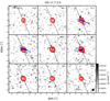 |
Fig. A.1. Same as Fig. 2, but for 29SiO v = 0, J = 5 − 4 emission around OH 17.7-2.0. The peak emission is I29SiO, peak = 0.31 Jy beam−1. The maximum polarisation fraction Pl, max = 4.7%. |
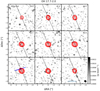 |
Fig. A.2. Same as Fig. 2, but for SiO v = 0, J = 5 − 4 emission around OH 17.7-2.0. The peak emission is ISiO, peak = 0.49 Jy beam−1 and the maximum polarisation fraction Pl, max = 2.9%. |
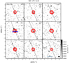 |
Fig. A.3. Same as Fig. 2, but for SO J = 5 − 4 emission around OH 17.7-2.0. The peak emission is ISO, peak = 0.12 Jy beam−1 and the maximum polarisation fraction Pl, max = 2.2%. |
All Tables
All Figures
|
Fig. 1. 222.5 GHz continuum emission from OH 17.7−2.0 in red contours. The contours are drawn at 0.625, 1.25, 2.5, 5, 10, 20, 40, and 80% of the peak value of 71.8 mJy beam−1. The dashed line indicates the direction of the outflow inferred from mid-infrared continuum and H2 observations (Gledhill et al. 2011). Left: the four labelled solid circles are the sources identified by Gaia within a radius of 2.5″ of OH 17.7−2.0 (see text). The greyscale also represents the continuum emission. Right: the polarised continuum emission (greyscale) of OH 17.7−2.0. The blue line segments indicate the linear polarisation direction where polarised emission is detected at > 3σ, where the rms on the polarised emission σ = 21 μJy beam−1. This means that the uncertainty on the direction is ≲10°. The segments are scaled by the linear polarisation fraction which peaks at Pl, max = 0.47%. The filled ellipse indicates the beam size of the observations. |
| In the text | |
|
Fig. 2. Channel maps of polarised CO J = 2 − 1 emission around the post-AGB star OH 17.7−2.0. The Stokes I total intensity emission is indicated by the solid red contours at 2.5, 5, 10, 20, 40, and 80% of the peak emission (ICO, peak = 1.04 Jy beam−1). The linearly polarised emission is shown as a greyscale map, and the blue line segments denote the linear polarisation direction when the polarised emission > 5σP. The uncertainty on the polarisation direction is thus ≲7°. The segments are scaled to the level of fractional polarisation with the scale indicated in the bottom left panel. The maximum polarisation Pl, max = 4.1%. The panels are labelled with the VLSR velocity in km s−1, and the beam size is shown in the bottom right panel. The stellar velocity VLSR, * = 62.0 km s−1. The dashed line indicates the direction of the outflow of OH 17.7−2.0, as in Fig. 1. |
| In the text | |
|
Fig. 3. Zoomed-in view of continuum emission (grey scale) of OH 17.7−2.0 with the blue line segments denoting the linear polarisation of CO J = 2 − 1 for the two channels around the systemic velocity (labelled in km s−1 in the top right corner). The dashed red line segments indicate the linear polarisation direction of the continuum polarisation. The black dashed line indicates the direction of the bipolar outflow. |
| In the text | |
|
Fig. 4. Zoomed-in view of central region of CO J = 2 − 1 emission previously shown in Fig. 2. The greyscale indicates the Stokes I emission and the blue line segments indicate the linearly polarisation direction. The red dashed contours represent the (negative) Stokes V emission at −8, −6, and −4σ, where σ = 0.4 mJy beam−1. The outflow direction is indicated by the dashed line. The blue box indicates the region of the 1612 MHz OH masers for which a linear polarisation map is presented in B03 (their Fig. 7). The majority of the OH masers are located within ∼0.4″ of the centre of the map. The channel velocity in km s−1 is given the top right corner of each panel. |
| In the text | |
|
Fig. 5. Dispersion of polarisation vectors (the square root of the second-order structure function) binned to the Nyquist sampled resolution, for two velocity channels of the CO J = 2 − 1 polarised emission around OH 17.7−2.0. The error bars indicate the variance in each bin. The vertical dotted line indicates the size of the beam major axis. The solid line indicates the fit of the structure function analysis described in the text. |
| In the text | |
|
Fig. 6. Distribution of absolute angle difference between 1612 MHz OH masers (B03) and CO polarisation direction. The mean difference, which can be affected by Faraday rotation, has been removed (see text). The solid black line indicates a normal distribution, and σ = 22.5°, which corresponds to the best-fit normal distribution. The dashed line represents a uniform distribution of angle differences. |
| In the text | |
|
Fig. A.1. Same as Fig. 2, but for 29SiO v = 0, J = 5 − 4 emission around OH 17.7-2.0. The peak emission is I29SiO, peak = 0.31 Jy beam−1. The maximum polarisation fraction Pl, max = 4.7%. |
| In the text | |
|
Fig. A.2. Same as Fig. 2, but for SiO v = 0, J = 5 − 4 emission around OH 17.7-2.0. The peak emission is ISiO, peak = 0.49 Jy beam−1 and the maximum polarisation fraction Pl, max = 2.9%. |
| In the text | |
|
Fig. A.3. Same as Fig. 2, but for SO J = 5 − 4 emission around OH 17.7-2.0. The peak emission is ISO, peak = 0.12 Jy beam−1 and the maximum polarisation fraction Pl, max = 2.2%. |
| In the text | |
Current usage metrics show cumulative count of Article Views (full-text article views including HTML views, PDF and ePub downloads, according to the available data) and Abstracts Views on Vision4Press platform.
Data correspond to usage on the plateform after 2015. The current usage metrics is available 48-96 hours after online publication and is updated daily on week days.
Initial download of the metrics may take a while.