| Issue |
A&A
Volume 697, May 2025
|
|
|---|---|---|
| Article Number | A206 | |
| Number of page(s) | 16 | |
| Section | Interstellar and circumstellar matter | |
| DOI | https://doi.org/10.1051/0004-6361/202450330 | |
| Published online | 21 May 2025 | |
Gas infall via accretion disk feeding Cepheus A HW2
1
INAF, Osservatorio Astronomico di Cagliari,
via della Scienza 5,
09047
Selargius,
Italy
2
Max-Planck-Institut für Radioastronomie,
Auf dem Hügel 69,
53121
Bonn,
Germany
3
Département d’Astronomie, Université de Genève,
Chemin Pegasi 51,
1290
Versoix,
Switzerland
4
Space Research Center (CINESPA), School of Physics, University of Costa Rica,
11501
San José,
Costa Rica
5
INAF-Osservatorio Astrofisico di Arcetri,
Largo E. Fermi 5,
50125
Firenze,
Italy
6
Instituto de Radioastronomía y Astrofísica UNAM,
Apartado Postal 3-72 (Xangari),
58089
Morelia, Michoacán,
Mexico
7
INAF – Istituto di Radioastronomia & Italian ALMA Regional Centre,
Via P. Gobetti 101,
40129
Bologna,
Italy
8
NRAO,
520 Edgemont Road,
Charlottesville,
VA
22903,
USA
9
Institut de Ciéncies de l’Espai (ICE-CSIC), Can Magrans s/n,
08193,
Bellaterra, Barcelona,
Spain
10
Institut d’Estudis Espacials de Catalunya (IEEC),
Barcelona,
Spain
11
Instituto de Astronomía Téorica y Experimental (IATE, CONICET-UNC),
Córdoba,
Argentina
12
INAF – Osservatorio Astronomico di Capodimonte,
salita Moiariello 16,
80131
Napoli,
Italy
13
Faculty of Physics, University of Duisburg-Essen,
Lotharstra β e 1,
47057
Duisburg,
Germany
★ Corresponding author: alberto.sanna@inaf.it
Received:
11
April
2024
Accepted:
19
February
2025
The star-forming region Cepheus A hosts a very young star, called HW2, that is the second closest to us growing a dozen times more massive than our Sun. The circumstellar environment surrounding HW2 has been the subject of extensive debate on the possible presence of an accretion disk, whose existence is at the foundation of our current paradigm of star formation. Here, we look to answer this long-standing question by resolving the gaseous disk component and its kinematics through sensitive observations at centrimetre (cm) wavelengths of hot ammonia (NH3) with the Jansky Very Large Array. We mapped the accretion disk surrounding HW2 at radii between 200 and 700 au, showing how fast circumstellar gas collapses and slowly orbits to pile up near the young star at very high rates of 2 × 10⁻³ M⊙ yr−1. These results, corroborated by state-of-the-art simulations, show that an accretion disk is still efficient in terms of focusing huge mass-infall rates near the young star, even after this star had already achieved a large mass of 16 M⊙.
Key words: circumstellar matter / stars: formation / stars: kinematics and dynamics / stars: massive / stars: protostars
© The Authors 2025
 Open Access article, published by EDP Sciences, under the terms of the Creative Commons Attribution License (https://creativecommons.org/licenses/by/4.0), which permits unrestricted use, distribution, and reproduction in any medium, provided the original work is properly cited.
This article is published in open access under the Subscribe to Open model. Subscribe to A&A to support open access publication.
1 Introduction
The large reservoir of interstellar gas needed to build up a massive star dozens of times more massive than our Sun is known to pile up over wide regions of the order of a parsec (pc). However, it is only within circumstellar regions as large as a few hundred astronomical units (au) across that the gas will be ultimately collected to accrete onto a ‘small’ proto-star, with diameter of only about a million kilometers. Resolving the properties of the gas flow as it streams in the inner region (of a few hundreds of au) from a very young star, it has been an observational challenge since a long time. This is especially true for the most massive stars that are found much further away from Earth than Solar-type stars (e.g., Cesaroni et al. 2007; Beltrán & de Wit 2016). The circumstellar regions where gas collapses onto a plane, and orbits faster as it is pulled inwards by the central star’s gravity, are generally referred to as the accretion disk, which is the physical structure that ultimately conveys mass onto Solar-type stars (e.g., Dauphas & Chaussidon 2011). In recent decades, this general picture of disk-mediated accretion has been much questioned when applied to the formation of massive stars, where a large mass reservoir of several tens of solar masses has to focus near the star and sustain mass infall rates exceeding 10−4 M⊙ yr−1. Under these conditions, the disk stability can be severely affected by local fragmentation, tidal interactions with nearby cluster members, and powerful stellar feedback, for example, as suggested both theoretically and observationally (e.g., Meyer et al. 2018; Oliva & Kuiper 2020; Maud et al. 2017; Goddi et al. 2020; Johnston et al. 2020; Sanna et al. 2021). As such, a general consensus has not been reached yet, even for those massive stars at smaller distances from the Sun.
At a trigonometric distance of 700 pc from the Sun (Moscadelli et al. 2009; Dzib et al. 2011), Cepheus A is the second-nearest star-forming site where massive young stars of ten (or more) solar masses are born (Kun et al. 2008). In the innermost regions of Cepheus A, there is an outstanding bright and compact radio source, called ‘HW2’ after Hughes & Wouterloot (Hughes & Wouterloot 1984; Garay et al. 1996; Rodriguez et al. 1994; Curiel et al. 2006), that was soon recognized to pinpoint a newly born massive star, whose own luminosity dominates that of the whole region of several thousands of solar luminosities (e.g., De Buizer et al. 2017). The environment surrounding HW2 has been the target of many studies aimed to verify star formation theories in past years, because its close distance to the Sun provides a preferred test laboratory. Nevertheless, these studies have been contradictory at the very least, some suggesting the presence of a circumstellar disk (e.g., Patel et al. 2005; Torrelles et al. 2007; Jiménez-Serra et al. 2009; Ahmadi et al. 2023) while others have attributed it to a chance superposition of different protostellar cores (e.g., Brogan et al. 2007; Comito et al. 2007). Ultimately, two main questions remain open, namely, whether HW2 forms via disk accretion or, alternatively, whether this lack challenges our understanding of how massive stars gather their large masses when they are still very young (e.g., Goddi et al. 2020).
In late spring 2019, we performed high-sensitivity Very Large Array (VLA) observations at wavelengths near 1 centimetre (cm) of the hot ammonia (NH3) line emission, which is excited in the circumstellar gas around HW2. When talking about hot gaseous ammonia, we are referring to emission from those transitions excited at kinetic temperatures above 100 K, such as the metastable (J = K) inversion transitions with J higher than 3 observable at radio wavelengths (e.g., Ho & Townes 1983). Their detection is a signpost of dense and warm gas heated in the vicinity of a young massive star (e.g., Cesaroni et al. 1992; Goddi et al. 2015). The idea behind this project is to search via hot ammonia for direct evidence of an accretion disk surrounding HW2 by resolving physical scales of the order of 100 au.
2 Observations and data reduction
We conducted spectroscopic VLA observations in band K (18.0–26.5 GHz) of the Galactic star-forming region Cepheus A. Observations were carried out under program 19A-248 on 2019 at four epochs of 2.5 hours each, on April 27, June 24, 26, and 27. The array used 27 antennas in B configuration to make observations during the first three epochs, with baselines approximately ranging from a minimum of 10 kλ to a maximum of 830 kλ. At the last epoch, the array started moving to the largest configuration with baselines extending up to 1.5 Mλ. Observation information is summarised in Table A.1.
We made use of a mixed correlator (WIDAR) set-up consisting of three basebands: a single baseband sampled at 8 bits and 1.0 GHz wide, along with two basebands sampled at three bits of 2.0 GHz each (Perley et al. 2011). These basebands were centred at frequencies of 24.170, 22.210, and 20.000 GHz, respectively. The first set-up was used to cover the NH3 (1, 1) to (5, 5) metastable inversion transitions (Table A.2) with five spectral windows, each 16 MHz wide, and 384 channels of 41.7 kHz. These settings provide a velocity coverage of 200 km s−1 near each line, wide enough to encompass their hyperfine structure, and a narrow velocity resolution of 0.5 km s−1 to sample the range of ammonia emission, of the order of 10 km s−1 (Torrelles et al. 2007). Spectral windows of 128 MHz and 64 channels were used to fill all basebands for the continuum measurement.
The VLA visibility data were calibrated with the Common Astronomy Software Applications (CASA) package version 5.3.0 (CASA Team 2022) and processed through the scripted pipeline (version 1.4.2, which uses the Perley-Butler 2017 flux density scale). Manual flagging was performed on each scheduling block separately. We imaged the five spectral line windows with the task tclean of CASA combining the four scheduling blocks and processing the uv-data with natural weightings to maximize the sensitivity to the ammonia emission. Image cubes were used to select the line-free channels from a spectrum integrated over a circular area of 3″ in size, which was centred on the target source. These channels were input into the task imcontsub of CASA to subtract a constant continuum level (fitorder = 0) from the image cubes, obtaining a continuum-free dataset for each ammonia line. All spectral line images discussed in the paper were obtained by applying natural weightings to maximize the array sensitivity and retrieve faint emission at increasing distances from the star. The image produced with continuum spectral windows was self calibrated to improve on the map dynamic range (peak of 11 mJy beam−1) and uses Briggs’s robust weightings (ℜ = 1) to minimize beam side lobes.
The synthesised beams are ![$\[0^{\prime\prime}_\cdot452 \times 0^{\prime\prime}_\cdot285\]$](/articles/aa/full_html/2025/05/aa50330-24/aa50330-24-eq1.png) at −75.8° and
at −75.8° and ![$\[0^{\prime\prime}_\cdot512 \times 0^{\prime\prime}_\cdot306\]$](/articles/aa/full_html/2025/05/aa50330-24/aa50330-24-eq2.png) at −71.9° for the line and continuum maps, respectively, with position angles measured east of north. The line imaging achieves a root-mean-square (rms) thermal noise of approximately 0.9 mJy beam−1 per resolution unit, corresponding to a brightness temperature of about 15 K at the given beam. Continuum imaging achieves a rms thermal noise of approximately 5 μJy beam−1, with the continuum central frequency set at 21.8 GHz.
at −71.9° for the line and continuum maps, respectively, with position angles measured east of north. The line imaging achieves a root-mean-square (rms) thermal noise of approximately 0.9 mJy beam−1 per resolution unit, corresponding to a brightness temperature of about 15 K at the given beam. Continuum imaging achieves a rms thermal noise of approximately 5 μJy beam−1, with the continuum central frequency set at 21.8 GHz.
3 Results
In Fig. 1, we present three plots summarizing the kinematic information inferred from the ammonia line imaging. Firstly, we identified three ranges of velocity, 5 to 6 km s−1 wide, which are associated with three different spatial distributions of gas near the young star. These velocities are referred to as the red-shifted (from +3.9 to −1.7 km s−1), systemic (from −2.24 to −7.3 km s−1), and blue-shifted ranges (from −7.8 to −12.9 km s−1). Altogether, they encompass the whole range of emission of dense molecular gas, from +4 to −13 km s−1 approximately, as reported in larger scale observations of the past (e.g., Jiménez-Serra et al. 2009, and references therein).
Beginning with the upper panel, we compared two maps of the NH3 (5, 5) emission integrated in velocity (i.e., a moment-zero map), which were obtained from two distinct velocity intervals taken consecutive (marked in red and white). The interval at higher velocities (red-dashed contours) is characterised by molecules observed in absorption only, whose peak is centred above the previously identified star position Curiel et al. (2006). These velocities are red-shifted with respect to the systemic velocity (Vsys) of the region at nearly −4.5 km s−1 (Sanna et al. 2017). In the upper and middle panels of Fig. 1, white contours are used to draw emission integrated over the velocity range centred on the systemic velocity and 6 km s−1 wide. This emission is characterized by two approximately symmetric lobes (hereafter, the bulk emission) to the south-east and north-west of the central absorption region, which is still visible at these velocities (white-dashed contours). In the red-shifted map, the absorption region has an elongated spatial morphology connecting the bulk emission to the south of the star position, with a deconvolved (Gaussian) size of ![$\[0^{\prime\prime}_\cdot26 \times 0^{\prime\prime}_\cdot6\]$](/articles/aa/full_html/2025/05/aa50330-24/aa50330-24-eq3.png) at a position angle of 101° ± 4°. In the middle panel, the integrated map at red-shifted velocities is replaced by one at blue-shifted (lower) velocities, where ammonia is observed in emission only (blue contours). The blue-shifted emission is characterized by an arched spatial morphology that bridges the bulk emission to the north of the star position.
at a position angle of 101° ± 4°. In the middle panel, the integrated map at red-shifted velocities is replaced by one at blue-shifted (lower) velocities, where ammonia is observed in emission only (blue contours). The blue-shifted emission is characterized by an arched spatial morphology that bridges the bulk emission to the north of the star position.
The bottom panel gives the full kinematic information of the bulk and blue-shifted velocities integrated together via a (coloured) first-moment map overplotted on moment-zero (black) contours. The moment-zero map shows a nearly complete ring of ammonia emission surrounding the absorption region: moving outward from the absorption centre, the ring has a minimum radius of nearly 200 au and can be detected up to radii between 600 and 700 au, at the current sensitivity (cf. linear scale in the panel). The first-moment map is evaluated within the 4 σ contour of the moment-zero map and its local weighted velocity is quantified by the colour scale to the right, ranging from −13.9 to −4.3 km s−1. There is a regular change seen in the gas velocity across the ring, whose apparent pattern is the combination of two velocity components, counterclockwise rotation, and infall motions, as explained later on in this work. We can show that a similar velocity pattern is observed with different ammonia lines at decreasing excitation energies, as proof of an intrinsic gas property (Fig. 2). The ammonia emission appears fainter to the south-west in correspondence to the red-shifted absorption, where it is only faintly detected through the (2, 2) and (4, 4) inversion lines showing a closed ring. In the following, we generally refer to the NH3 molecular ring as the accretion disk.
We can demonstrate that the accretion disk encircles the region near HW2 where the bright radio emission was discovered by overplotting maps of ammonia and centimeter continuum (Fig. B.1). The latter is a tracer of thermal bremsstrahlung emission from hydrogen gas ionized along a protostellar jet. This radio thermal jet is a prototypical example of the kind that was first resolved in the early 1990s (Rodriguez et al. 1994), recently shown to arise at physical scales of only 20 au from HW2 (Carrasco-González et al. 2021). The correspondence between the molecular ring centre with the bright radio continuum from the protostellar jet provides direct explanation for the ammonia absorption, which arises from gas distributed further away from the star and in foreground against the continuum. This feature, as well as others discussed in the following sections, are explained in the cartoon in Fig. 3.
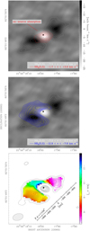 |
Fig. 1 Accretion disk in ammonia surrounding HW2 (black star). Top: moment zero maps of the (5, 5) inversion line evaluated within two velocity ranges, as indicated on the bottom right (beam size on the bottom panel). White contours and grey background quantify the line brightness about the systemic velocity, whereas the red-dashed contours the red-shifted absorption observed against the central region. Contours start at 3 σ increasing by 1 σ of 1.8 mJy beam−1 km s−1; dashed (negative) contours start at −3 σ decreasing by 2 σ. Middle: similar to the top panel, but with the moment zero map at red-shifted velocities replaced by one at blue-shifted velocities. Bottom: moment zero (black contours) and first moment (colours) maps obtained by combining the systemic and blue-shifted ranges, with velocities quantified by the colour wedge to the right. Same contour levels as the upper panels, with 1 σ of 2.6 mJy beam−1 km s−1. A linear scale is drawn along a position angle of 134° east of north and all panels show the same field. |
NH3 line fitting
To derive the physical conditions of ammonia gas, we made use of the brightness ratio between three inversion transitions, the (2, 2), (4, 4), and (5, 5). Their state belongs to the subgroup of NH3 molecules whose hydrogen spins are antiparallel, that are named para-NH3 and correspond to quantum numbers K ≠ 3n (n an integer). Alternatively, states with all hydrogen spins parallel are named ortho-NH3 (K = 3n). Changes of spin orientation are not allowed via radiative or collisional transitions, which makes of para- and ortho-NH3 two distinct species that do not mix (e.g., Ho & Townes 1983). For this reason, the (3, 3) inversion transition was neglected from the spectral fitting. For our purposes, emission coming from the (1, 1) inversion transition was also excluded due to its low excitation energy, of only 23.8 K, which implies heavy contamination from cold gas belonging to the diffuse envelope at large distances from the star (e.g., Mangum et al. 2013).
We extracted three spectra per transition from three distinct circular areas with a diameter equal to the beam major axis (of 316 au), which optimises the signal-to-noise ratio (S/N) and angular resolution (Fig. 4). We drew the best fit to the line passing through the absorption peak and the peaks of the bulk emission and centred the pointings along this line. To compare the lobes of the bulk emission, two pointings were equally spaced by 380 au from the absorption peak, where a third pointing was set (grey shades in Fig. 4). The spectral resolution was Hanning-smoothed to improve on the sensitivity.
In Figs. A.1 and A.2, we plot four spectra, including the (3, 3) inversion transition, to emphasise the existence of two overlapping velocity components at the position of absorption, which were detected both in the para- and ortho-species (single components detected elsewhere). Each spectrum shows similar properties consisting of two blended peaks of absorption, between −8 and +4 km s−1, with a first component peaking near the negative systemic velocity (Vsys) and a second component at positive red-shifted velocities. These two components are treated separately in the following. Notably, in Fig. A.1 we also plot theoretical positions of the satellite hyperfine lines of NH3 for each velocity component (green and magenta separately), as computed from analytic formulas in Kisliuk & Townes (1950). Hyperfines are neglected in the following because they are heavily affected by the noise, which prevents their positive detection and fit.
We applied the same approach for spectral fitting followed by Sanna et al. (2021), which also accounts for the continuum level. Firstly, we searched for best guesses of the gas physical conditions by means of Weeds, a package of the Grenoble Image and Line Data Analysis Software (GILDAS – Maret et al. 2011). We sought to reproduce the NH3 spectra both in emission and absorption. Weeds generates synthetic spectra of a given molecular species whose energy levels are populated by thermal distribution, after fixing five parameters: (i) the intrinsic full width at half maximum (FWHM) of the spectral lines; (ii) the line offset with respect to the rest velocity in the region; (iii) the spatial extent (FWHM) of the emitting region, approximated to a Gaussian brightness profile; (iv) the rotational temperature; and (v) the column density of the emitting gas. Parameters (i) and (ii) were tested separately by fitting a Gaussian profile to each inversion line.
Secondly, we processed the initial parameters into MCWeeds exploiting a Bayesian statistical analysis for an automated fit of the spectral lines (Giannetti et al. 2017). We minimised the difference between the observed and computed spectra via Monte Carlo Markov chains, deriving the best-fit parameters with their statistical uncertainties. To reproduce the central absorption, we set the background continuum temperature based on the 22.2 GHz flux density inside the pointing area (of 7.3 mJy), but we assigned an effective size equal to the A-array beam (of 80 mas). In doing so, we accounted for the fact that 22.2 GHz observations by Curiel et al. (2006) detected same peak fluxes (within uncertainties) at the resolution of the longest VLA baselines, which is evidence of compact emission. This assumption is further supported by the fit convergence a posteriori.
The following (standard) caveats also apply. Synthetic spectra were produced under the working hypothesis of a single excitation temperature and column density (per velocity component) and were assumed to be uniform along the line-of-sight; on the contrary, the latter crosses portions of gas at different distances from the star, where we would otherwise expect a smooth change in the gas physical conditions (e.g., streamline in Fig. 3). Different transitions are also forced to have same linewidth, assuming that each spectral component is excited within the same parcel of gas. These approximations will be disregarded in our analysis due to the negligible discrepancies between observed and fitted line profiles.
In Table A.3, we list the results of the NH3 spectral fitting for the three pointings to the eastern side, western side, and in front of the young star (column 1). Columns 2 and 3 quantify the (projected) linear distance of each pointing from the star position and extent of the integrated areas, respectively. Columns 4 to 7 list the best fit parameters of the gas emission output by MCWeeds with their statistical uncertainties. Column 8 specifies the opacity computed by Weeds for the NH3 (5, 5) line imaged in the main figures. In Fig. A.2, we also show the same absorption spectra of Fig. A.1, but also include the continuum level for completeness.
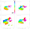 |
Fig. 2 Comparison of the NH3 gas kinematic among the inversion lines from (2, 2) to (5, 5), as indicated in the top left with upper excitation energies. Each panel shows a first-moment map of a given line (colour map) with overplotted its moment zero contours. Moments are calculated over the same velocity range (see Fig. 1) and the velocity scale is quantified by the colour wedge in the top left panel. Positive contours start at 3 σ and increase by 1 σ of 2.6 mJy beam−1 km s−1; negative (dashed) contours start at −3 σ by steps of −2 σ. The first-moment maps are evaluated within the 4 σ contour of their moment zero map; the thick red contour draws the 3 σ contour of the NH3 (5, 5) map for comparison with other lines. Same field of view and resolution as in Fig. 1 (beam size shown in the top-left panel). |
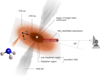 |
Fig. 3 Cartoon of the star formation scenario around HW2, where the observer is placed to the right for clarity. The line-of-sight to HW2, slightly above the disk mid-plane by 26° (Sanna et al. 2017), crosses a column of NH3 gas infalling in front of a region of bright continuum emission, confined inside the inner 200 au. At larger radii, the observer maps emission from NH3 gas (molecular structure sketched to the left), which is both infalling (vr) by gravity toward the central star and rotating (vϕ) at sub-Keplerian velocities. Atomic (ionised) gas is also ejected away along the general direction of the system angular momentum, with a lobe of blue-shifted (approaching to the observer) gas to the north and one of red-shifted (receding) gas to the south (e.g., Gómez et al. 1999). |
4 Discussion
The relative brightness of the centimeter ammonia lines provides a sensitive thermometer for the circumstellar gas, as emission at different excitation energies can be used to find the best description for the gas conditions locally, under the assumption of thermodynamic equilibrium (e.g., Ho & Townes 1983; Walmsley & Ungerechts 1983; Mangum et al. 2013). This assumption is satisfied at the high particle densities (in excess of 107 cm−3) expected around a massive star across its equatorial plane, at radii of thousands of au and below (e.g., Sanna et al. 2021). In Fig. 4, we summarise this analysis based on the line brightness ratio of the (2, 2), (4, 4), and (5, 5) ammonia para lines. At the frequency of each ammonia transition, we produced integrated spectra extracted from three pointings placed at the peaks of emission and absorption (grey circles in Fig. 4), which are representative of gas seen at the two opposite sides with respect to the central star and along its direction, respectively (the latter sketched in Fig. 3). In the contour map of Fig. 4, we also show that the spatial extent of ammonia correlates with the morphology of the dust emission (red contours) imaged at comparable resolution by Beuther et al. (2018), likely indicating copious evaporation from dust grain mantles where the ammonia molecules are synthesized. As an example, the side panels in Fig. 4 display spectra of the (5, 5) transition at the higher excitation temperature of 296 K, whereas the blue profiles draw the final synthetic spectra obtained from the line fitting (best-fit parameters in the corners).
The spectral line fitting delivers twofold information, about the NH3 physical conditions and its kinematics as well (Table A.3). Firstly, at the eastern and western sides of the accretion disk, at an average radius of 380 au from the central star, gas is warmed up to comparable temperatures of approximately 170 K, although the eastern side attains twice as much column (thus material) and linewidth than the western side. This discrepancy cannot be reconciled even within a 3 σ uncertainty. This finding was already noticed in the past and interpreted as evidence of two distinct hot molecular cores, with information lacking on the kinematic pattern of gas at high angular resolution (Brogan et al. 2007; Comito et al. 2007). Our observations can now separate the line emission and absorption properly and probe a continuous physical structure instead. In turn, these results suggest a much higher gas turbulence on one disk side, which (as we show below) has a counterpart in the smoothed velocity gradient observed to the east of the star than to the west (see Sect. 4.1).
Secondly, by looking through the column of NH3 gas directly in front of the young star, we can distinguish two, blended, velocity components, whose peak velocities are both red-shifted with respect to the systemic velocity and whose physical conditions differ. Labeled ‘component 2’, the most red-shifted component (by 5.7 km s−1) is warmer and has a column density almost two times larger than the colder, less red-shifted component (by 0.4 km s−1), labeled as ‘component 1’. This evidence suggests we are probing two different portions of gas that overlap along the line-of-sight, with the warmer (closer to the star) gas component infalling at higher velocities in the star direction than the colder component. This scenario of infalling gas can be better understood when we add the kinematic information coming from the first-moment ammonia map, which, in turn, provides a second indirect proof of infall and is discussed in the following section.
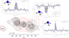 |
Fig. 4 Gas physical conditions near HW2. Bottom left: spatial extent of the NH3 (5, 5) bulk emission (black contours, same as Fig. 1) as compared to the dust emission (red contours) mapped in continuum at 1.37 mm by Beuther et al. (2018). Red contours start from a threshold of 27 mJy beam−1 increasing by a factor 2. The equatorial reference frame is rotated clockwise by 44° to align the (projected) outflow direction with the vertical axis of the plot (linear scale to the bottom). Large grey spots mark the loci where side spectra were integrated. Side panels: spectra of the local NH3 (5, 5) emission (grey histograms) extracted at the position of the peaks of emission and absorption. In each panel, the blue profile draws the best fit spectrum to the NH3 emission with fitted parameters of excitation temperature (T) and column density (N) written in the corners. The systemic velocity (Vsys) of circumstellar gas is marked with a red, vertical, dotted line and the 3D molecular structure is sketched. |
4.1 Kinematic toy model
In order to interpret the kinematic pattern of NH3 gas around HW2, we have built up a toy model presented in the right panel of Fig. 5. This model reproduces the velocity field of an ideal, razor-thin disk that has a radius comparable to the extent of the ammonia emission (700 au) and where we mask out the inner region of absorption (200 au). The local velocity vector computed from the model is the composition of two free parameters of counterclockwise rotation and radial motion of gas collapse. The magnitudes of rotation and infall are given as fractions of the local values of Keplerian (vK) and free-fall (vf f) velocities, respectively, which only depend on the gravitational field strength centrally. The observer measures the velocity component projected along the line-of-sight (VLSR), via the line’s Doppler shift, which we analytically derive after taking into account the orientation of the disk plane in space (by setting the disk inclination, i = 64°, and position angle, P.A. = 134°, estimated from Sanna et al. 2017). For a direct comparison with observations, we also (i) accounted for the same systemic velocity, (ii) we smoothed the velocity pattern spatially within a kernel equal to the beam size, and (iii) only plotted the range of integrated velocities exploited in the first-moment map.
We searched for couples of rotation (vϕ) and infall (vr) values whose line-of-sight projection reproduces the observed first-moment map. Their values were chosen among realistic combinations of Keplerian (VKep) and free-fall (Vff) fractions, respectively, whose magnitudes are functions of the disk radius and the central mass only. The analysis was carried out by considering two possible values for the central mass inside the absorption region, of 12 and 16 M⊙, which best fit the spectral energy distribution towards Cepheus A, as measured by De Buizer et al. (2017).
In Figs. A.3 and A.4, we show a number of combinations for the percentage of Keplerian and free-fall velocities producing a given kinematic pattern along the line-of-sight (VLSR). These combinations explain how the VLSR changes across the ring by increasing (and decreasing) either one or the other quantity. There are two characteristic features that constrain the underlying velocity field once the central mass is known, namely, the position angle of the region of (relatively) bluish emission and the magnitude of the line-of-sight velocities. We explicitly note that according to the colour scaled used, regions of reddest emission are those where the line-of-sight velocity is comparable to the systemic velocity (of −4.5 km s−1) and, thus, the gas motion in the local standard of rest is nearly zero along the line of sight. As a rule of thumb, we note that: (1) when decreasing the percentage of Keplerian velocity, the bluish region of emission shifts clockwise along the ring; whereas (2) when increasing the percentage of free-fall velocity, the bluish velocities increase in absolute magnitude. Our observations show that bluish velocities are bracketed inside the second quadrant with an abrupt reddish gradient crossing over the first quadrant (Fig. 2).
This qualitative analysis shows that each different combination of infall and rotation around HW2 produces an unique velocity pattern, which can be compared with the observations to explain the gas motion around the young star. At first sight, this comparison allows us to exclude, for instance, the possibility of fast rotation close to centrifugal equilibrium for radii larger than 200 au, while it also implies the existence of large infall motions dominating the gas kinematics at this distance from the star. In particular, in the right panel of Fig. 5, we list the set of parameters that best match the observed ammonia map (left panel). The ammonia pattern is reproduced for gas that is collapsing close to free-fall and rotating at 40% (±10%) the Keplerian value at a given radius. In fact, by assuming higher fractions of Keplerian rotation, bluish velocities largely encompass the third quadrant as well, which is at variance with observations; whereas values lower than 30% the Keplerian rotation underestimate the region of bluish emission (Figs. A.3 and A.4). Our toy model also supports that the velocity magnitudes can be better reproduced by setting a central mass of 16 M⊙ (Fig. A.4), as opposed to a smaller value of 12 M⊙ which fails to (Fig. A.3). Accordingly, De Buizer et al. (2017) obtained lower χ2 fitting values for a stellar mass of 16 M⊙ than 12 M⊙, by modelling the spectral energy distribution from Cepheus A.
To further support the model consistency, in the left panel of Fig. A.5 we show the full range of velocities predicted to the south-west of the star position, where the absorption feature suggests strongly red-shifted motions. According to the toy model, in this spatial region the local velocity vector should be almost aligned with the line of sight and oriented away from the observer, with velocities higher than −2.5 km s−1 and below +5 km s−1 approximately. This expected velocity range corresponds to that covered by the ammonia absorption, in agreement with our observation (Fig. A.1).
Interestingly, looking at the left panel of Fig. 5, the third quadrant shows a much smoother velocity gradient than the first quadrant, as compared to the model expectations to the right. This finding is directly related to the broad linewidths detected on the eastern side of the accretion disk with respect to the western narrow linewidths. Because both disk sides have similar temperatures, this difference in linewidth has to be related to a higher degree of gas turbulence on the eastern side. Moreover, the higher gas column density on the eastern disk side indicates a gas density approximately twice as high, assuming that the disk structure is mostly uniform all around and that the relative abundance between NH3 and H2 molecules is comparable on both disk sides. We suggest that the cause behind this difference might be an external injection of mass to the eastern disk side. In this scenario, the accretion disk must be continuously replenished of fresh material to sustain the ongoing mass infall towards HW2. Indeed, in the recent literature, there is growing evidence to support streamlines of gas and dust, referred to as streamers, connecting the inner circumstellar regions of young stars with the surrounding envelope (e.g., Akiyama et al. 2019; Pineda et al. 2020; Garufi et al. 2022). In this respect, and in support of our hypothesis, we note that a clear streamline of molecular gas is evident in the sub-arcsecond millimeter maps by Ahmadi et al. (2023, in particular, in their Figs. 2 and A.1). This emission appears to connect with the eastern side of the accretion disk surrounding HW2.
Finally, we explicitly recall that the purpose of the toy model represented in Fig. 5 is to reproduce the pattern of velocities observed in ammonia with basic assumptions. These assumptions cannot account for the spatial morphology and brightness of ammonia emission whose explanations (in terms of physical and environmental conditions) goes beyond the scope of the current toy model. On the contrary, this toy model is highly valuable in guiding us to constrain a ‘more realistic’ scenario, discussed via independent simulations in the following.
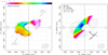 |
Fig. 5 Comparison between observations (left panel) and a toy model (right panel) which reproduces the line-of-sight velocity pattern of ammonia. Left: same as the bottom panel of Fig. 1, but with the axes labelled in astronomical units and offsets counted from the star position. A grid is drawn at steps of 200 au for a direct comparison with the right panel and the quadrants are labelled. The third quadrant shows a velocity gradient that is much smoother than in the first quadrant due to ammonia linewidths being twice as broad (Fig. 4). Right: similar to the left panel, but with the colour map obtained from the toy model of a razor thin disk with the same geometry of circumstellar gas around HW2 and convolved with the same instrumental beam. Model parameters are written in the top-left, with the velocity vectors sketched in the fourth quadrant. |
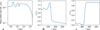 |
Fig. 6 Kinematic properties of the accretion disk according to the simulation that resembles our observations the most, taken after t = 9.62 kyr from its beginning. From left to right, the panels show the dependence with radius of the (a) mass infall rate, the (b) azimuthal velocity as a fraction of the Keplerian value, and the (c) radial velocity as a fraction of the free-fall value. |
4.2 Simulations
Notably, we find that the kinematic pattern observed around HW2 is indeed predicted by recent ab initio simulations of the formation of stars as massive as HW2. In order to provide a theoretical ground validating our interpretation independently, we searched a recently published catalog of numerical simulations (Oliva & Kuiper 2023a,b). These simulations start from the gravitational collapse of a cloud core threaded by an uniform magnetic field initially, whose outcome will ultimately be a massive (proto)star surrounded by an accretion disk and a magnetically driven outflow. The gas and dust were modelled along with the stellar evolution (Hosokawa & Omukai 2009) by accounting for non-ideal magneto-hydrodynamic effects (Mignone et al. 2007), Ohmic dissipation (Machida et al. 2007), self-gravity (Kuiper et al. 2010), and radiation transport approximated via gray flux-limited diffusion (Kuiper et al. 2020). The spatial domain was sampled through an axis-symmetric grid in spherical coordinates, with 224 and 40 cells in the radial and polar directions, respectively, and increasing the radial dimension logarithmically with distance.
Simulations in the catalog explore several possible precollapse conditions for massive star formation, varying the initial mass of the cloud, density and angular momentum distributions, and the initial magnetic field strength. In order to identify a set of simulations approximating our observations more closely, we constrained candidates to have an accreted stellar mass similar to HW2, with a Keplerian disk size equal or smaller than 200 au, as well as to drive a highly collimated jet. The best match was found for an initial cloud core of 100 M⊙ enclosed within 0.1 pc, whose density distribution is a power law with radius as ρ ∝ r−2. The angular momentum is calculated assuming initial solid body rotation with a rotational-to-gravitational-energy ratio of 4%. The initial magnetic field strength is set to 68 μG corresponding to a mass-to-flux ratio of 20 times the critical value (below which magnetic fields prevent collapse).
The steep density profile triggers the cloud to rapidly collapse when the system is left to evolve freely, while the angular momentum transport towards the centre slowly builds up an accretion disk. After 9.62 kyr from the start, the young star has already reached a mass of 16 M⊙, which is consistent with that of HW2. Despite the high stellar mass, the system is still young (i.e., without photo-ionization) because of the strong accretion rates reached at this early stage that, in turn, depend on the initial conditions of the collapse. The current mass of the accretion disk amounts to 2.2 M⊙ within a radius of 700 au, of which 1.6 M⊙ is enclosed within a Keplerian radius of 240 au only, indicating a disk-to-star mass ratio of 10–14%. This conclusion is in good agreement with recent estimates of the inner gas mass surrounding HW2, between 0.8–2.6 M⊙, obtained through interferometric observations of millimeter dust emission (Beuther et al. 2018; Gieser et al. 2021; Ahmadi et al. 2023).
In Figs. 6 and 7, we plot a number of results from the selected simulation for comparison. Beginning with Fig. 6, the left panel (a) shows the theoretical mass infall rate calculated along the equatorial plane as a function of the radial distance from the star, whose values are in excellent agreement with our measurement of 2.0 · 10−3 M⊙ yr−1 (see below). In the middle panel (b) of the same figure, we show the percentage of Keplerianity with radius. The flow in the innermost ~250 au of the disk is nearly Keplerian and decreases to 30–40% the Keplerian value for radii between 400 and 700 au, in good agreement with our findings. In the right panel (c), we plot the radial velocity of gas as a function of the disk radius. A decrease in Keplerianity corresponds a steep increase of the radial component of gas collapse, which approaches theoretical free-fall at 300 au, which is in good agreement with our observations. Finally, in Fig. 7 we present a 3D synthetic image of the velocity along the line-of-sight (vLSR), tracing material surrounding the young star within 700 au and using a similar colour scale as in Fig. 5. In the spatial range traced by ammonia emission (and absorption), the simulations, toy model, and observations are all consistent with each other. In particular, the left panel of Fig. 7 shows the sharp transition in the disk pattern where the gas kinematics changes from a sub-Keplerian regime to a Keplerian one within about 200 au from the star. For completeness, in the right panel of Fig. A.5, we also show the full kinematic pattern of gas around the young star, tracing the higher velocities (in absolute value) that are associated with the inner Keplerian rotation.
5 Mass infall rate in the inner disk regions
Having information about the magnitude of infall velocity at a given disk radius, together with the physical conditions of local gas, we are in a position to calculate the amount of gas mass crossing the disk per unit time towards the central star, as follows. We first considered a flow of mass, M, and average density, ρ, moving through a spherical shell with radius, R, and thickness, dR, over a time interval, dt. The total mass crossing the shell per unit time is, ![$\[\dot{\text{M}}=4 ~\pi ~\text{R}^{2} \cdot(\mathrm{dR} / \mathrm{dt}) \cdot \rho\]$](/articles/aa/full_html/2025/05/aa50330-24/aa50330-24-eq4.png) . Now, we consider an inward motion with vr = dR/dt that only flows through a small solid angle Ω, such as the opening angle of a flared disk. Then, we can rewrite
. Now, we consider an inward motion with vr = dR/dt that only flows through a small solid angle Ω, such as the opening angle of a flared disk. Then, we can rewrite ![$\[\dot{\text{M}}\]$](/articles/aa/full_html/2025/05/aa50330-24/aa50330-24-eq5.png) in convenient units:
in convenient units:
![$\[\left[\frac{\dot{\mathrm{M}}_{\mathrm{in}}}{\mathrm{M}_{\odot} ~\mathrm{yr}^{-1}}\right]=1.5 \cdot 10^{-4}\left[\frac{\mathrm{R}}{100 ~\mathrm{au}}\right]^2 \cdot\left[\frac{\mathrm{v}_{\mathrm{r}}}{10 \mathrm{~km} \mathrm{~s}^{-1}}\right] \cdot\left[\frac{\mathrm{n}_{\mathrm{H}_2}}{10^8 \mathrm{~cm}^{-3}}\right] \cdot\left[\frac{\Omega}{4 \pi}\right],\]$](/articles/aa/full_html/2025/05/aa50330-24/aa50330-24-eq6.png) (1)
(1)
where nH2 refers to the volume density of molecular hydrogen, which is the most abundant molecule by orders of magnitude.
In Eq. (1), each variable can be quantified based on the results of our observations. We solve Eq. (1) for a distance Rx = 380 au at the position of our western measurement of NH3 physical conditions. At this distance from the star, the theoretical free-fall velocity amounts to 8.6 km s−1. To estimate the volume density of molecular hydrogen at Rx, we refer to the sketch in Fig. A.6 and reason as follows. As a common assumption, we consider a flared disk where the ratio between the disk height (Hi) at varying radii (Ri) is constant, ![$\[\frac{\mathrm{H}_{\mathrm{i}}}{\mathrm{R}_{\mathrm{i}}}=\tan \alpha=K\]$](/articles/aa/full_html/2025/05/aa50330-24/aa50330-24-eq7.png) . The disk height along the line-of-sight through Rx is:
. The disk height along the line-of-sight through Rx is: ![$\[\mathrm{H}_{\mathrm{x}}=\sqrt{\mathrm{R}_{\mathrm{x}}^{2}+\mathrm{x}^{2}}\]$](/articles/aa/full_html/2025/05/aa50330-24/aa50330-24-eq8.png) . K, which depends on the projection x along the disk plane. Alternatively, we can write the ratio between Hx and x as:
. K, which depends on the projection x along the disk plane. Alternatively, we can write the ratio between Hx and x as:
![$\[\frac{\mathrm{H}_{\mathrm{x}}}{\mathrm{x}}=\tan \theta=\sqrt{1+\frac{\mathrm{R}_{\mathrm{x}}^2}{\mathrm{x}^2}} \cdot \mathrm{~K}.\]$](/articles/aa/full_html/2025/05/aa50330-24/aa50330-24-eq9.png) (2)
(2)
Notably, the right hand side of this equation is always greater than K, meaning that (1) the angle θ is greater than α, which is the flaring angle, and (2) θ increases as the projection x decreases. Also, x has an upper limit set by the geometry of the ammonia disk (RNH3 = 700 au) and the position of our measurement (Rx = 380 au), so that, ![$\[\mathrm{x}_{\text {max }}=\sqrt{\mathrm{R}_{\mathrm{NH}_{3}}^{2}-\mathrm{R}_{\mathrm{x}}^{2}}=587 ~\mathrm{au}\]$](/articles/aa/full_html/2025/05/aa50330-24/aa50330-24-eq10.png) and tan θ = 1.19 · K. Thus, we can calculate an upper limit to the disk path crossed by the line-of-sight through the Rx position, of:
and tan θ = 1.19 · K. Thus, we can calculate an upper limit to the disk path crossed by the line-of-sight through the Rx position, of:
![$\[2 \times \text{p}_\text{x}<2 \cdot \frac{\text{x}_{\max }}{\cos ~26^{\circ}}=1306 ~\mathrm{au},\]$](/articles/aa/full_html/2025/05/aa50330-24/aa50330-24-eq11.png) (3)
(3)
where the factor of 2 accounts for both positive and negative heights with respect to the disk mid-plane. In conclusion, by dividing the (lower) western column density of 3.98 · 1016 cm−2 for this path and accounting for a NH3-to-H2 abundance ratio of 3 · 10−9, we derive a lower limit to the local H2 volume density of 6.8 · 108 cm−3. The abundance ratio is a conservative upper limit inferred by comparing the higher value of NH3 column, of 7.08 · 1016 cm−2, with the peak column density of molecular hydrogen, of 2.1 · 1025 cm−2, as measured at comparable resolution through millimeter continuum emission (Beuther et al. 2018, their Table A.1).
The column of warm ammonia gas that we have detected in absorption along the line-of-sight comprises gas coming from an outer disk layer above the mid-plane by 26° (Figs. 3 and A.6). Its column density is more rarefied by an order of magnitude than that of the emission measured by looking through the disk plane directly (at Rx = 380 au in Fig. A.6), although the path intercepted by the line-of-sight to the centre is of the same order of magnitude as pmax. This evidence suggests that the disk should be flared by an opening angle of Ω ≤ 2 × 26° ≈ 60°.
Finally, plugging in these numbers in Eq. (1), we find that at an average distance of 380 au from the star, the inward stream of gas, flowing at a radial velocity of 8.6 km s−1, induces a mass infall rate of 2.0 · 10−3 M⊙ yr−1. This result only decreases by a factor of 1.5 when replacing the theoretical free-fall velocity with the peak value of the most red-shifted component measured along the line of sight (Table A.3) of 5.7 km s−1 (being the line-of-sight average).
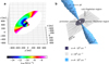 |
Fig. 7 3D view of the accretion disk kinematics as obtained from the selected simulation, taken after t = 9.62 kyr from its beginning. To the left, panel (a) shows the theoretical pattern of line-of-sight velocities within a similar range as Fig. 5 for a direct comparison, including also the inner disk regions where the rotation curve becomes Keplerian (masked by absorption in our observations). To the right, panel (b) shows the entire disk and jet structures produced by the selected simulation, where the reference levels of hydrogen volume density are listed for the accretion disk (Keplerian and sub-Keplerian regions separately) and the jet. |
6 Conclusions
We report on spectroscopic, B-configuration Jansky Very Large Array (VLA) observations of hot ammonia emission near 1 cm towards Cepheus A HW2. We targeted the metastable inversion transitions up to the (5, 5) line and map a ring of ammonia gas between radii of about 700 au and down to 200 au from HW2, as part of its accretion disk. Ammonia is detected both in emission and absorption, the latter seen in foreground against the bright radio continuum of the radio thermal jet driven by HW2.
We resolved the gas kinematics across the ring which we interpret via both a toy model and a direct comparison with independent ab initio simulations. This analysis shows that the velocity field traced by ammonia is a composition of slow rotation and prominent infall motions that still overtake centrifugal equilibrium at disk radii of only a few hundreds of au. At this distance from the star, gas slowly orbits at a few 10% the Keplerian value around a central mass of 16 M⊙, which is consistent with the spectral energy distribution from the region. In particular, our simulations predict a similar scenario as observed around HW2 when the system is still very young, of the order of 10 kyr, and a Keplerian regime is only reached in the innermost 200 au accordingly.
We measured the ammonia physical conditions across the ring by fitting together the (2, 2), (4, 4), and (5, 5) ammonia para lines and inferring gas temperatures above 170 K for disk radii smaller than 380 au. This analysis also suggests a higher degree of gas turbulence on one disk side than to the other, which might be related to a streamer of dense gas detected in previous millimeter observations of Cepheus A. In particular, we analytically derived the mass infall rate of gas streaming through the disk at a radius of 380 au, whose high value of 2 × 10⁻³ M⊙ yr−1 is in agreement with what the prediction given in our independent simulations.
Finally, we recall that two independent detections of luminosity bursts have been reported from as many young and massive stars (Caratti o Garatti et al. 2017; Hunter et al. 2017). These observations are proof of episodic events of stellar accretion, where a circumstellar disk can suddenly convey a mass as high as a few Jupiter masses (≈ 3 × 10⁻³ M⊙) onto the star. If these findings imply the existence of an accretion disk indirectly, they also require the mass infall rates to be of the same order of the accreted mass. Indeed, we can prove observationally that similar infall rates can be efficiently sustained by an accretion disk, such as the one we observe around the nearby HW2. In doing so, we have been able to settle a dispute that has long questioned the existence of an accretion disk around one of the closest massive forming stars to the Sun and which has also (because of HW2’s preferred position) cast doubt on the accretion mechanism itself.
Acknowledgements
Comments from an anonymous referee, which helped improving our paper, are gratefully acknowledged. This paper makes use of data obtained with the Karl G. Jansky Very Large Array, operated by the National Radio Astronomy Observatory (NRAO). The NRAO is a facility of the National Science Foundation operated under cooperative agreement by Associated Universities, Inc. This paper makes use of the Grenoble Image and Line Data Analysis Software (GILDAS) – https://www.iram.fr/IRAMFR/GILDAS. A.S. acknowledges financial support from the INAF-Minigrant 2022 “Feasibility project for the ngVLA: a Science Case with Masers” (ngVLAmas, P.I.: A. Sanna). A.O. acknowledges financial support from the State Secretariat for Education, Research and Innovation of the Swiss Confederation via their program “Swiss Government Excellence Scholarships for Foreign Students 2023/2024”, the Office of International Affairs and External Cooperation of the University of Costa Rica, and the European Research Council (ERC) under the European Union’s Horizon 2020 research and innovation program (grant agreement No. 833925, project STAREX). C.C.-G. acknowledges support from UNAM DGAPA-PAPIIT grant IG101224 and from CONAHCyT Ciencia de Frontera project ID 86372. G.S acknowledges the project PRIN-MUR 2020 MUR BEYOND-2p “Astrochemistry beyond the second period elements” (Prot. 2020AFB3FX) and the INAF-Minigrant 2023 “TRacing the chemIcal hEritage of our originS: from proTostars to planEts” (TRIESTE, PI: G. Sabatini). J.M.T. acknowledges partial support from the PID2023-146675NB grant funded by MCIN/AEI/10.13039/501100011033, and by the program Unidad de Excelencia María de Maeztu CEX2020-001058-M. A.C.G. acknowledges support from PRIN-MUR 2022 20228JPA3A “The path to star and planet formation in the JWST era” (PATH) funded by NextGeneration EU, by INAF-GoG 2022 “NIR-dark Accretion Outbursts in Massive Young stellar objects” (NAOMY), and by Large Grant INAF 2022 “YSOs Outflows, Disks and Accretion: towards a global framework for the evolution of planet forming systems” (YODA).
Appendix A Additional material
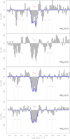 |
Fig. A.1 Integrated spectra of the NH3 line emission (gray) evaluated over the central absorption region. From top to bottom are displayed spectra of the inversion lines from (2, 2) to (5, 5) as labelled on the bottom right. The absorption feature near the systemic velocity of the region, indicated with a dotted red line (Vsys), is the combination of two, distinct, velocity components. Theoretical positions of the satellite hyperfine lines (HF) are approximately indicated for both components in green and magenta separately, whereas the blue profile draws the best fit spectrum to the ammonia para lines. |
VLA settings for experiment 19A-248 observed during spring and early summer 2019.
Observed ammonia lines.
Physical parameters obtained by fitting the NH3 spectra between 23-25 GHz.
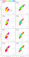 |
Fig. A.3 Different fractions of Keplerian (vKep) and free-fall (vff) velocities which can affect the appearance of the kinematic pattern observed in ammonia, assuming a central mass of 12 M⊙. Same symbols as in Fig. 5. |
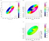 |
Fig. A.5 Full velocity field of circumstellar gas around HW2, as predicted by the toy model (panel a) and the simulations (panels b and c). These plots are produced under the same conditions as in the right panel of Fig. 5 (for the toy model) and Fig. 7a (for the simulations), but show the full range of gas velocities expected theoretically. In particular, in panel a), velocities coloured from orange to magenta cover the range of absorption observed in the ammonia spectra. Panel b) shows the simulated velocities plotted with the same colour scale of the toy model to the left, for comparison. We explicitly note that the toy model and simulations predict consistent velocities with each other (cf. Figs. 5 and 7a). Panel c) shows the simulated velocities with a larger velocity range, to include the innermost and fastest (Keplerian) velocities not covered by the toy model. |
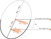 |
Fig. A.6 Sketch for calculating the maximum path of the NH3 column density measured by an observer who is looking through the disk at different positions. For instance, when an observer to the right looks at the position Rx on the eastern disk side, its line-of-sight crosses a path which is 2 × px long, where the angle θ is always greater than the flaring angle α. |
Appendix B Radio continuum
In Fig. B.1 we present a summary of the radio continuum imaging. The top panel shows the appearance of the continuum map at 1.3 cm, as obtained from the line free channels of the current ammonia dataset. The middle panel shows the spectral index map of the continuum at 1.3 cm in the region of ammonia absorption, where the nominal uncertainty is better than 0.01 thanks to the high signal-to-noise ratio. The lower panel shows the appearance of the continuum map at 3.6 cm from archival data (Curiel et al. 2002), whose angular resolution is two times better than that of the upper panel and whose absolute position has been registered for the secular motion of the star forming region (as derived from Moscadelli et al. 2009). The spectral index map, generated following Sanna et al. (2018), shows values between −0.1 and 0.5, as expected for a radio thermal jet. This result confirms that the bright continuum background, against which ammonia lines are observed in absorption, originates from the compact ejected gas driven by HW2 (Carrasco-González et al. 2021).
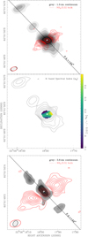 |
Fig. B.1 Thermal radio jet emission (grey shades) driven by HW2 (white star) compared with the spatial distribution of the NH3 emission (red contours). Top: radio continuum emission at 1.3 cm (K band), obtained from the same NH3 dataset, overplotted on the (5, 5) inversion line emission near the systemic velocity. Radio continuum levels start at 7 σ increasing by factors of 2 (1 σ of 5 μJy beam−1). The dotted black line traces the mean jet axis at a position angle of 44° for comparison. Synthesized beams on the bottom left. Middle: In-band spectral index map (colours) measured from the K-band radio continuum (black contours, same as upper panel). Values according to the colour wedge to the right. Bottom: Similar to the upper panel but for the radio continuum emission at 3.6 cm (X band; see Appendix B) and a field of view two times smaller. Radio continuum levels start at 5 σ increasing at steps of 3 σ (1 σ of 36 μJy beam−1). |
References
- Ahmadi, A., Beuther, H., Bosco, F., et al. 2023, A&A, 677, A171 [NASA ADS] [CrossRef] [EDP Sciences] [Google Scholar]
- Akiyama, E., Vorobyov, E. I., Liu, H. B., et al. 2019, AJ, 157, 165 [NASA ADS] [CrossRef] [Google Scholar]
- Beltrán, M. T., & de Wit, W. J. 2016, A&A Rev., 24, 6 [CrossRef] [Google Scholar]
- Beuther, H., Mottram, J. C., Ahmadi, A., et al. 2018, A&A, 617, A100 [NASA ADS] [CrossRef] [EDP Sciences] [Google Scholar]
- Brogan, C. L., Chandler, C. J., Hunter, T. R., Shirley, Y. L., & Sarma, A. P. 2007, ApJ, 660, L133 [Google Scholar]
- Caratti o Garatti, A., Stecklum, B., Garcia Lopez, R., et al. 2017, Nat. Phys., 13, 276 [Google Scholar]
- Carrasco-González, C., Sanna, A., Rodríguez-Kamenetzky, A., et al. 2021, ApJ, 914, L1 [CrossRef] [Google Scholar]
- CASA Team (Bean, B., et al.) 2022, PASP, 134, 114501 [NASA ADS] [CrossRef] [Google Scholar]
- Cesaroni, R., Walmsley, C. M., & Churchwell, E. 1992, A&A, 256, 618 [NASA ADS] [Google Scholar]
- Cesaroni, R., Galli, D., Lodato, G., Walmsley, C. M., & Zhang, Q. 2007, in Protostars and Planets V, eds. B. Reipurth, D. Jewitt, & K. Keil, 197 [Google Scholar]
- Comito, C., Schilke, P., Endesfelder, U., Jiménez-Serra, I., & Martín-Pintado, J. 2007, A&A, 469, 207 [NASA ADS] [CrossRef] [EDP Sciences] [Google Scholar]
- Curiel, S., Trinidad, M. A., Cantó, J., et al. 2002, ApJ, 564, L35 [Google Scholar]
- Curiel, S., Ho, P. T. P., Patel, N. A., et al. 2006, ApJ, 638, 878 [NASA ADS] [CrossRef] [Google Scholar]
- Dauphas, N., & Chaussidon, M. 2011, Annu. Rev. Earth Planet. Sci., 39, 351 [Google Scholar]
- De Buizer, J. M., Liu, M., Tan, J. C., et al. 2017, ApJ, 843, 33 [Google Scholar]
- Dzib, S., Loinard, L., Rodríguez, L. F., Mioduszewski, A. J., & Torres, R. M. 2011, ApJ, 733, 71 [NASA ADS] [CrossRef] [Google Scholar]
- Garay, G., Ramirez, S., Rodriguez, L. F., Curiel, S., & Torrelles, J. M. 1996, ApJ, 459, 193 [NASA ADS] [CrossRef] [Google Scholar]
- Garufi, A., Podio, L., Codella, C., et al. 2022, A&A, 658, A104 [CrossRef] [EDP Sciences] [Google Scholar]
- Giannetti, A., Leurini, S., Wyrowski, F., et al. 2017, A&A, 603, A33 [NASA ADS] [CrossRef] [EDP Sciences] [Google Scholar]
- Gieser, C., Beuther, H., Semenov, D., et al. 2021, A&A, 648, A66 [EDP Sciences] [Google Scholar]
- Goddi, C., Zhang, Q., & Moscadelli, L. 2015, A&A, 573, A108 [NASA ADS] [CrossRef] [EDP Sciences] [Google Scholar]
- Goddi, C., Ginsburg, A., Maud, L. T., Zhang, Q., & Zapata, L. A. 2020, ApJ, 905, 25 [NASA ADS] [CrossRef] [Google Scholar]
- Gómez, J. F., Sargent, A. I., Torrelles, J. M., et al. 1999, ApJ, 514, 287 [CrossRef] [Google Scholar]
- Ho, P. T. P. & Townes, C. H. 1983, ARA&A, 21, 239 [NASA ADS] [CrossRef] [Google Scholar]
- Hosokawa, T., & Omukai, K. 2009, ApJ, 691, 823 [Google Scholar]
- Hughes, V. A., & Wouterloot, J. G. A. 1984, ApJ, 276, 204 [NASA ADS] [CrossRef] [Google Scholar]
- Hunter, T. R., Brogan, C. L., MacLeod, G., et al. 2017, ApJ, 837, L29 [NASA ADS] [CrossRef] [Google Scholar]
- Jiménez-Serra, I., Martín-Pintado, J., Caselli, P., et al. 2009, ApJ, 703, L157 [CrossRef] [Google Scholar]
- Johnston, K. G., Hoare, M. G., Beuther, H., et al. 2020, A&A, 634, L11 [NASA ADS] [CrossRef] [EDP Sciences] [Google Scholar]
- Kisliuk, P. P., & Townes, C. H. 1950, J. Res. Natl. Bureau Standards, 44, 611 [Google Scholar]
- Kuiper, R., Klahr, H., Beuther, H., & Henning, T. 2010, ApJ, 722, 1556 [NASA ADS] [CrossRef] [Google Scholar]
- Kuiper, R., Yorke, H. W., & Mignone, A. 2020, ApJS, 250, 13 [Google Scholar]
- Kun, M., Kiss, Z. T., & Balog, Z. 2008, Star Forming Regions in Cepheus, ed. B. Reipurth, 136 [Google Scholar]
- Machida, M. N., Inutsuka, S.-i., & Matsumoto, T. 2007, ApJ, 670, 1198 [NASA ADS] [CrossRef] [Google Scholar]
- Mangum, J. G., Darling, J., Henkel, C., et al. 2013, ApJ, 779, 33 [CrossRef] [Google Scholar]
- Maret, S., Hily-Blant, P., Pety, J., Bardeau, S., & Reynier, E. 2011, A&A, 526, A47 [NASA ADS] [CrossRef] [EDP Sciences] [Google Scholar]
- Maud, L. T., Hoare, M. G., Galván-Madrid, R., et al. 2017, MNRAS, 467, L120 [NASA ADS] [Google Scholar]
- Meyer, D. M. A., Kuiper, R., Kley, W., Johnston, K. G., & Vorobyov, E. 2018, MNRAS, 473, 3615 [NASA ADS] [CrossRef] [Google Scholar]
- Mignone, A., Bodo, G., Massaglia, S., et al. 2007, ApJS, 170, 228 [Google Scholar]
- Moscadelli, L., Reid, M. J., Menten, K. M., et al. 2009, ApJ, 693, 406 [NASA ADS] [CrossRef] [Google Scholar]
- Oliva, G. A., & Kuiper, R. 2020, A&A, 644, A41 [NASA ADS] [CrossRef] [EDP Sciences] [Google Scholar]
- Oliva, A., & Kuiper, R. 2023a, A&A, 669, A80 [NASA ADS] [CrossRef] [EDP Sciences] [Google Scholar]
- Oliva, A., & Kuiper, R. 2023b, A&A, 669, A81 [NASA ADS] [CrossRef] [EDP Sciences] [Google Scholar]
- Patel, N. A., Curiel, S., Sridharan, T. K., et al. 2005, Nature, 437, 109 [CrossRef] [Google Scholar]
- Pearson, J. C., Müller, H. S. P., Pickett, H. M., Cohen, E. A., & Drouin, B. J. 2010, J. Quant. Spec. Radiat. Transf., 111, 1614 [NASA ADS] [CrossRef] [Google Scholar]
- Perley, R. A., Chandler, C. J., Butler, B. J., & Wrobel, J. M. 2011, ApJ, 739, L1 [Google Scholar]
- Pineda, J. E., Segura-Cox, D., Caselli, P., et al. 2020, Nat. Astron., 4, 1158 [NASA ADS] [CrossRef] [Google Scholar]
- Rodriguez, L. F., Garay, G., Curiel, S., et al. 1994, ApJ, 430, L65 [NASA ADS] [CrossRef] [Google Scholar]
- Sanna, A., Moscadelli, L., Surcis, G., et al. 2017, A&A, 603, A94 [NASA ADS] [CrossRef] [EDP Sciences] [Google Scholar]
- Sanna, A., Moscadelli, L., Goddi, C., Krishnan, V., & Massi, F. 2018, A&A, 619, A107 [NASA ADS] [CrossRef] [EDP Sciences] [Google Scholar]
- Sanna, A., Giannetti, A., Bonfand, M., et al. 2021, A&A, 655, A72 [NASA ADS] [CrossRef] [EDP Sciences] [Google Scholar]
- Torrelles, J. M., Patel, N. A., Curiel, S., et al. 2007, ApJ, 666, L37 [Google Scholar]
- Walmsley, C. M., & Ungerechts, H. 1983, A&A, 122, 164 [Google Scholar]
All Tables
VLA settings for experiment 19A-248 observed during spring and early summer 2019.
All Figures
|
Fig. 1 Accretion disk in ammonia surrounding HW2 (black star). Top: moment zero maps of the (5, 5) inversion line evaluated within two velocity ranges, as indicated on the bottom right (beam size on the bottom panel). White contours and grey background quantify the line brightness about the systemic velocity, whereas the red-dashed contours the red-shifted absorption observed against the central region. Contours start at 3 σ increasing by 1 σ of 1.8 mJy beam−1 km s−1; dashed (negative) contours start at −3 σ decreasing by 2 σ. Middle: similar to the top panel, but with the moment zero map at red-shifted velocities replaced by one at blue-shifted velocities. Bottom: moment zero (black contours) and first moment (colours) maps obtained by combining the systemic and blue-shifted ranges, with velocities quantified by the colour wedge to the right. Same contour levels as the upper panels, with 1 σ of 2.6 mJy beam−1 km s−1. A linear scale is drawn along a position angle of 134° east of north and all panels show the same field. |
| In the text | |
|
Fig. 2 Comparison of the NH3 gas kinematic among the inversion lines from (2, 2) to (5, 5), as indicated in the top left with upper excitation energies. Each panel shows a first-moment map of a given line (colour map) with overplotted its moment zero contours. Moments are calculated over the same velocity range (see Fig. 1) and the velocity scale is quantified by the colour wedge in the top left panel. Positive contours start at 3 σ and increase by 1 σ of 2.6 mJy beam−1 km s−1; negative (dashed) contours start at −3 σ by steps of −2 σ. The first-moment maps are evaluated within the 4 σ contour of their moment zero map; the thick red contour draws the 3 σ contour of the NH3 (5, 5) map for comparison with other lines. Same field of view and resolution as in Fig. 1 (beam size shown in the top-left panel). |
| In the text | |
|
Fig. 3 Cartoon of the star formation scenario around HW2, where the observer is placed to the right for clarity. The line-of-sight to HW2, slightly above the disk mid-plane by 26° (Sanna et al. 2017), crosses a column of NH3 gas infalling in front of a region of bright continuum emission, confined inside the inner 200 au. At larger radii, the observer maps emission from NH3 gas (molecular structure sketched to the left), which is both infalling (vr) by gravity toward the central star and rotating (vϕ) at sub-Keplerian velocities. Atomic (ionised) gas is also ejected away along the general direction of the system angular momentum, with a lobe of blue-shifted (approaching to the observer) gas to the north and one of red-shifted (receding) gas to the south (e.g., Gómez et al. 1999). |
| In the text | |
|
Fig. 4 Gas physical conditions near HW2. Bottom left: spatial extent of the NH3 (5, 5) bulk emission (black contours, same as Fig. 1) as compared to the dust emission (red contours) mapped in continuum at 1.37 mm by Beuther et al. (2018). Red contours start from a threshold of 27 mJy beam−1 increasing by a factor 2. The equatorial reference frame is rotated clockwise by 44° to align the (projected) outflow direction with the vertical axis of the plot (linear scale to the bottom). Large grey spots mark the loci where side spectra were integrated. Side panels: spectra of the local NH3 (5, 5) emission (grey histograms) extracted at the position of the peaks of emission and absorption. In each panel, the blue profile draws the best fit spectrum to the NH3 emission with fitted parameters of excitation temperature (T) and column density (N) written in the corners. The systemic velocity (Vsys) of circumstellar gas is marked with a red, vertical, dotted line and the 3D molecular structure is sketched. |
| In the text | |
|
Fig. 5 Comparison between observations (left panel) and a toy model (right panel) which reproduces the line-of-sight velocity pattern of ammonia. Left: same as the bottom panel of Fig. 1, but with the axes labelled in astronomical units and offsets counted from the star position. A grid is drawn at steps of 200 au for a direct comparison with the right panel and the quadrants are labelled. The third quadrant shows a velocity gradient that is much smoother than in the first quadrant due to ammonia linewidths being twice as broad (Fig. 4). Right: similar to the left panel, but with the colour map obtained from the toy model of a razor thin disk with the same geometry of circumstellar gas around HW2 and convolved with the same instrumental beam. Model parameters are written in the top-left, with the velocity vectors sketched in the fourth quadrant. |
| In the text | |
|
Fig. 6 Kinematic properties of the accretion disk according to the simulation that resembles our observations the most, taken after t = 9.62 kyr from its beginning. From left to right, the panels show the dependence with radius of the (a) mass infall rate, the (b) azimuthal velocity as a fraction of the Keplerian value, and the (c) radial velocity as a fraction of the free-fall value. |
| In the text | |
|
Fig. 7 3D view of the accretion disk kinematics as obtained from the selected simulation, taken after t = 9.62 kyr from its beginning. To the left, panel (a) shows the theoretical pattern of line-of-sight velocities within a similar range as Fig. 5 for a direct comparison, including also the inner disk regions where the rotation curve becomes Keplerian (masked by absorption in our observations). To the right, panel (b) shows the entire disk and jet structures produced by the selected simulation, where the reference levels of hydrogen volume density are listed for the accretion disk (Keplerian and sub-Keplerian regions separately) and the jet. |
| In the text | |
|
Fig. A.1 Integrated spectra of the NH3 line emission (gray) evaluated over the central absorption region. From top to bottom are displayed spectra of the inversion lines from (2, 2) to (5, 5) as labelled on the bottom right. The absorption feature near the systemic velocity of the region, indicated with a dotted red line (Vsys), is the combination of two, distinct, velocity components. Theoretical positions of the satellite hyperfine lines (HF) are approximately indicated for both components in green and magenta separately, whereas the blue profile draws the best fit spectrum to the ammonia para lines. |
| In the text | |
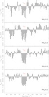 |
Fig. A.2 Similar to Fig. A.1 but with the continuum level included for comparison. |
| In the text | |
|
Fig. A.3 Different fractions of Keplerian (vKep) and free-fall (vff) velocities which can affect the appearance of the kinematic pattern observed in ammonia, assuming a central mass of 12 M⊙. Same symbols as in Fig. 5. |
| In the text | |
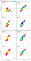 |
Fig. A.4 Similar to Fig. A.3, but for a central mass of 16 M⊙. |
| In the text | |
|
Fig. A.5 Full velocity field of circumstellar gas around HW2, as predicted by the toy model (panel a) and the simulations (panels b and c). These plots are produced under the same conditions as in the right panel of Fig. 5 (for the toy model) and Fig. 7a (for the simulations), but show the full range of gas velocities expected theoretically. In particular, in panel a), velocities coloured from orange to magenta cover the range of absorption observed in the ammonia spectra. Panel b) shows the simulated velocities plotted with the same colour scale of the toy model to the left, for comparison. We explicitly note that the toy model and simulations predict consistent velocities with each other (cf. Figs. 5 and 7a). Panel c) shows the simulated velocities with a larger velocity range, to include the innermost and fastest (Keplerian) velocities not covered by the toy model. |
| In the text | |
|
Fig. A.6 Sketch for calculating the maximum path of the NH3 column density measured by an observer who is looking through the disk at different positions. For instance, when an observer to the right looks at the position Rx on the eastern disk side, its line-of-sight crosses a path which is 2 × px long, where the angle θ is always greater than the flaring angle α. |
| In the text | |
|
Fig. B.1 Thermal radio jet emission (grey shades) driven by HW2 (white star) compared with the spatial distribution of the NH3 emission (red contours). Top: radio continuum emission at 1.3 cm (K band), obtained from the same NH3 dataset, overplotted on the (5, 5) inversion line emission near the systemic velocity. Radio continuum levels start at 7 σ increasing by factors of 2 (1 σ of 5 μJy beam−1). The dotted black line traces the mean jet axis at a position angle of 44° for comparison. Synthesized beams on the bottom left. Middle: In-band spectral index map (colours) measured from the K-band radio continuum (black contours, same as upper panel). Values according to the colour wedge to the right. Bottom: Similar to the upper panel but for the radio continuum emission at 3.6 cm (X band; see Appendix B) and a field of view two times smaller. Radio continuum levels start at 5 σ increasing at steps of 3 σ (1 σ of 36 μJy beam−1). |
| In the text | |
Current usage metrics show cumulative count of Article Views (full-text article views including HTML views, PDF and ePub downloads, according to the available data) and Abstracts Views on Vision4Press platform.
Data correspond to usage on the plateform after 2015. The current usage metrics is available 48-96 hours after online publication and is updated daily on week days.
Initial download of the metrics may take a while.