| Issue |
A&A
Volume 697, May 2025
|
|
|---|---|---|
| Article Number | A107 | |
| Number of page(s) | 19 | |
| Section | Numerical methods and codes | |
| DOI | https://doi.org/10.1051/0004-6361/202449619 | |
| Published online | 12 May 2025 | |
Deep learning interpretability analysis for carbon star identification in Gaia DR3
1
Department of Physics, Hebei Normal University,
Shijiazhuang
050024,
China
2
Guo Shoujing Institute for Astronomy, Hebei Normal University,
Shijiazhuang
050024,
China
3
CAS Key Laboratory of Optical Astronomy, National Astronomical Observatories,
Beijing
100101,
China
4
University of Chinese Academy of Sciences,
Beijing
100049,
China
5
Nanjing Institute of Astronomy and Optical Technology, University of Chinese Academy of Sciences,
Nanjing
211135,
China
6
School of Physics, Astronomy and Mathematics, University of Hertfordshire,
College Lane,
Hatfield
AL10 9AB,
UK
★ Corresponding authors; This email address is being protected from spambots. You need JavaScript enabled to view it.
; This email address is being protected from spambots. You need JavaScript enabled to view it.
; This email address is being protected from spambots. You need JavaScript enabled to view it.
Received:
15
February
2024
Accepted:
17
December
2024
Abstract
Context. A large fraction of asymptotic giant branch (AGB) stars develop carbon-rich atmospheres during their evolution. Based on their color and luminosity, these carbon stars can easily be distinguished from many other kinds of stars. However, numerous G, K, and M giants also occupy the same region as carbon stars on the HR diagram. Despite this fact, their spectra exhibit differences, especially in the prominent CN molecular bands.
Aims. We aim to distinguish carbon stars from other kinds of stars using Gaia’s XP spectra while providing attributional interpretations of key features that are necessary for identification and even discovering new key spectral features.
Methods. We propose a classification model named “GaiaNet”, an improved one-dimensional convolutional neural network specifically designed for handling Gaia’s XP spectra. We utilized SHapley Additive exPlanations (SHAP), an approach for interpretability based on game theoretic, to determine SHAP values for each feature in a spectrum, enabling us to explain the output of the GaiaNet model and provide further meaningful analysis.
Results. Compared to four traditional machine learning methods, the GaiaNet model exhibits an average classification accuracy improvement of approximately 0.3% on the validation set, with the highest accuracy reaching 100%. Utilizing the SHAP model, we present a clear spectroscopic heatmap highlighting molecular band absorption features primarily distributed around CN773.3 and CN895.0, and we summarize five key feature regions for carbon star identification. Upon applying the trained classification model to the CSTAR sample with Gaia “xp_sampled_mean” spectra, we obtained 451 new candidate carbon stars as a by-product.
Conclusions. Our algorithm is capable of discerning subtle feature differences from low-resolution spectra of Gaia, thereby assisting us in effectively identifying carbon stars with typically higher temperatures and weaker CN features while providing compelling attributive explanations. The interpretability analysis of deep learning holds significant potential in spectral identification.
Key words: methods: analytical / methods: data analysis / catalogs
© The Authors 2025
 Open Access article, published by EDP Sciences, under the terms of the Creative Commons Attribution License (https://creativecommons.org/licenses/by/4.0), which permits unrestricted use, distribution, and reproduction in any medium, provided the original work is properly cited.
This article is published in open access under the Subscribe to Open model. This email address is being protected from spambots. You need JavaScript enabled to view it. to support open access publication.
1 Introduction
Carbon stars, first recognized by Secchi (1869), exhibit an inversion of the C/O ratio (C/O > 1). In contrast to other stars, carbon stars possess carbon-enriched atmospheres. The enrichment can originate from mass transfer in binary systems or the activation of the third dredge-up (TDU) process during their asymptotic giant branch (AGB) evolution phase (Gaia Collaboration 2023). The carbon stars that arise in binary systems likely inherited atmospheric carbon through mass transfer from their AGB companion, which has since evolved into a white dwarf (Abia et al. 2002). These carbon stars are known as “extrinsic” carbon stars. However, the carbon enrichment of cool and luminous carbon stars (N-type) is caused by the pollution of nuclear helium fusion products transported from the inner to the outer layers during their AGB phase (Gaia Collaboration 2023). This process transports carbon from the interior region to the stellar surface, leaving the outer layers rich in carbon-containing molecules and dust particles. Thus, their spectra show C2 and CN molecular bands stronger than usual in stars cooler than 3800 K (i.e., GBP − GRP ≥ 2; Gaia Collaboration 2023). These carbon stars are called “intrinsic” carbon stars.
The spectra of carbon stars exhibit absorption characteristics due to carbon-containing compounds of CH, C2, and CN. The presence and intensity of these spectral features provide valuable insights into the atmospheric conditions and chemical processes within these stars. Because they tend to be in a late evolution stage of stellar mass loss, carbon stars are important contributors to the interstellar medium and serve as a good references for studying a variety of physical processes that affect the end of the life of low-mass stars (Gaia Collaboration 2023).
Traditionally, identifying and classifying carbon stars relied on parametric measurements and manual checking of their spectra. Ji et al. (2016) identified 894 carbon stars from the Large Sky Area MultiObject Fiber Spectroscopy Telescope (LAMOST) DR2 by measuring multiple line indices from the stellar spectra. Abia et al. (2022) reported the identification of 2660 new carbon star candidates through 2MASS photometry, Gaia astrometry, and their location in the Gaia–2MASS diagram. Li et al. (2023) distinguished carbon stars from M-type giants by selecting spectral indices satisfying the criterion [CaH3 − 0.8 × CaH2 − 0.1]< 0. Gaia Collaboration (2023) screened carbon stars by measuring the carbon molecular band head strength, resulting in a final selection of 15 740 high-quality “golden sample” carbon stars. Lebzelter et al. (2023) classified 546 468 carbon star candidates using a method guided by narrow-band photometry (Palmer & Wing 1982). Their specific object study (SOS) module examines this feature in an automated way by computing the pseudo-wavelength difference between the two highest peaks in each Gaia DR3 RP spectrum, taking the median value of the results and storing it in the parameter of median_delta_wl_rp. They assumed all stars with median_delta_wl_rp> 7 to be C-rich stars. Li et al. (2024) identified 3546 carbon stars through line indices and near-infrared color-color diagrams. Through visual inspection of these spectra, they further subclassified them into C−H, C−R, C−N, and Ba stars.
To date, many machine learning methods have been used to identify carbon stars based on their spectra. Si et al. (2014) applied the label propagation algorithm to search for 260 new carbon stars from the Sloan Digital Sky Survey (SDSS) DR8. Si et al. (2015) applied the efficient manifold ranking algorithm to search for 183 carbon stars from the LAMOST pilot survey. Li et al. (2018) identified 2651 carbon stars in the spectra of more than seven million stars using an efficient machine learning algorithm for LAMOST DR4. Sanders & Matsunaga (2023) investigated the use of unsupervised learning algorithms to classify the chemistry of long-period variables (Lebzelter et al. 2023) from Gaia DR3’s BP/RP spectra (also called XP spectra; Carrasco et al. 2021) into O-rich and C-rich groups. They also employed a supervised approach to separate O-rich and C-rich sources using broadband optical and infrared photometry. In all, they tagged a total of 23 737 C-rich classifications based on the BP/RP spectra and identified a small population of C-rich stars in the Galactic bar-bulge region.
In recent years, the application of interpretable analysis techniques in astronomy has shown great potential. Qin et al. (2019) used a random forest (RF) algorithm deriving rank features, then picked out 15 269 Am candidates from the early-type stars of LAMOST DR5. He et al. (2022) successfully distinguished between red giant branch (RGB) and red clump (RC) stars using the XGBoost algorithm (Chen & Guestrin 2016) and used the SHAP interpretable model (Lundberg & Lee 2017) to obtain the top features that the XGBoost selected. Shang et al. (2022) used machine learning algorithms to search for class-one and class-two chemical peculiars (CP1 and CP2). Finally, they presented a catalog of 6917 CP 1 and 1652 CP 2 new candidate sources using XGBoost followed by the visual investigation and listed the spectral features for separating CP1 from CP2 using SHAP.
Before this work, searching for carbon stars based on Gaia spectra was mainly done by obtaining the matching giant star spectra with an RF classifier (Breiman 2001) and then screening out carbon stars with strong CN molecular bands by measuring the molecular band head strength (Gaia Collaboration 2023). Most of the carbon stars identified in this manner belong to the N-type. Although this method can easily pick out the carbon stars with obvious spectral features, it misses those that exhibit relatively weak molecular bands. These carbon stars are mixed with non-carbon stars in the band head strength diagrams, which makes it difficult to identify them using this method. As an improvement of the method, our proposed algorithm can be used to identify the carbon stars that exhibit relatively weak molecular bands from their spectra in a quantitative manner.
In this work, we explore the significant potential of a deep learning model enhanced with the SHAP algorithm for identifying carbon stars using their Gaia DR3 XP spectra. In Sect. 2, we cover the source of the data, the preparation of the training set, and the data processing methods. In Sect. 3, we introduce the proposed deep learning classification model, important model parameters, the SHAP interpretability model, and the evaluation index. In Sect. 4, we show how well the model performs with a validation set and how it compares to other classification models, demonstrating the effectiveness of the model interpretation and key features as well as the newly discovered carbon star candidates. In Sect. 5, we compare the results with others, and we analyze and interpret the spectral features. Finally, a general summary is provided in Sect. 6.
2 Data
2.1 CSTAR sample of Gaia DR3
Gaia Data Release 3 (Gaia DR3) has been released in 2022, and its mean BP/RP spectral data was released in May of the same year, including four folders on the archive: rvs_mean_spectrum, xp_continuous_mean_spectrum, xp_sampled_mean_spectrum and xp_summary. The spectra we adopt are from xp_sampled_mean_spectrum1, which has 34 468 373 BP/RP externally calibrated sampled mean spectra. All mean spectra were sampled to the same set of absolute wavelength positions, viz. 343 values from 336 to 1020 nm with a step of 2 nm (i.e., corresponding to a wavelength range of 3360 to 109 200 Å in steps of 20 Å). To standardize the data scale range, we normalized the raw spectral data as
![Mathematical equation: $\[x^*=\frac{x-x_{\min }}{x_{\max }-x_{\min }},\]$](/articles/aa/full_html/2025/05/aa49619-24/aa49619-24-eq1.png) (1)
(1)
where x represents the original spectrum, the xmin and xmax respectively indicate the minimum and maximum value of the x, and the normalized spectrum is denoted as x*.
Min-max normalization is a data standardization method that maps the data to a 0–1 range in equal proportion, thus changing the distribution of the raw data. It only scales the spectrum without altering its original structural representation. It also accelerates the convergence rate of the deep learning model’s loss function, thereby enhancing the efficiency and speed of achieving the optimal solution, which might otherwise be hard to converge.
Gaia Collaboration (2023) (hereafter referred to as C2023) released a batch of “golden samples”, which include the “golden sample” of carbon stars. Their ESP-ELS module attempted to flag these suspected carbon stars. The module is based on a RF classifier trained on the synthetic BP and RP spectra and a sample of Galactic carbon stars (Abia et al. 2020) obtained from the Gaia low-resolution spectra (R = λ/δλ ≈ 25–100; Carrasco et al. 2021). In total, 386 936 targets received the “CSTAR” tag (i.e., the potential carbon star candidates). However, most of these stars are M stars rather than carbon stars, with only a small fraction exhibiting significant C2 and CN molecular bands. The majority of candidate carbon stars have GBP − GRP > 2 mag and have colors consistent with M stars (Gaia Collaboration 2023).
As shown in Table 1, C2023 considered four molecular band heads in order to further screen for reliable carbon stars. Finally, they selected 15 740 golden sample carbon stars based on the strongest CN molecular band features. Most of these golden sample carbon stars are AGB stars where the enriched carbon was produced and then dredged up from its interior region. In other words, they are cold and bright N-type carbon stars. The calculation formula for the four molecular band head strengths is as follows:
![Mathematical equation: $\[R_{\lambda_2}=\frac{f\left(\lambda_2\right)}{g_{\lambda_1, \lambda_3}\left(\lambda_2\right)},\]$](/articles/aa/full_html/2025/05/aa49619-24/aa49619-24-eq2.png) (2)
(2)
where f (λ2) is the flux measured at the top of the band head of the molecular band, and gλ1, λ3 is the value linearly interpolated between wavelengths λ1 and λ3 (Gaia Collaboration 2023).
The reason C 2023 did not select C2 molecular band strengths as filtering criterion may be twofold: firstly, the C2 features in the spectra are significantly weaker compared to CN features; secondly, more than half of the golden sample carbon stars lack prominent C2 features in their spectra after visual inspection. Therefore, C2 features lack clear distinction, as can also be seen in the band head strengths diagram of Fig. 4.
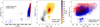 |
Fig. 1 Main parameters of CSTAR_XPM sample. Panel a: Teff and log g diagram of CSTAR_XPM. Panel b: Spatial location and density distribution of CSTAR_XPM and random sample in the GBP − GRP and log g plane. The random sample (gray) is randomly selected from xp_sampled_mean. CSTAR_XPM stars are located in the giant star branch, with most having 2 < GBP − GRP < 5 mag; Panel c shows the distribution of golden sample carbon stars (red) and non-golden sample carbon stars (blue) in CSTAR_XPM. |
Four molecular band head positions used to identify carbon stars.
2.2 Training data
After cross-matching the source_id of CSTAR with the spectral data of the xp_sampled_mean_spectrum library in Gaia DR3, we obtained 83 028 spectra. These spectra were used to verify the feasibility of our algorithm, which we refer to as CSTAR_XPM (CSTAR sample with xp_sampled_mean spectra). Of these, 8288 belong to the 15 740 golden sample of carbon stars and 74 740 are non-golden sample. We respectively refer to them as CSTAR_XPM_G (for the golden sample of CSTAR_XPM) and CSTAR_XPM_nonG (for the non-golden sample of CSTAR_XPM).
Considering that the Teff provided by Gaia DR3 may not be reliable, in Fig. 1, we also plotted the GBP − GRP (not dereddened) and log g diagrams of all CSTAR_XPM in order to get a basic idea of the physical properties and evolutionary state of these sources. Since a large proportion of the sources are missing Teff and log g, we plotted 3245 CSTAR_XPM_G sources, 47 290 CSTAR_XPM_nonG sources, and 6763 random sample sources. It is clear that the CSTAR_XPM_nonG and CSTAR_XPM_G are spatially intermingled in the distribution and are difficult to distinguish from each other.
From the panel a and c of Fig. 1, we noted that a few targets (19) of CSTAR_XPM_G have a log g greater than 3 and Teff hotter than 6000 K. However, their GBP − GRP is around 3, and their spectra are typical of AGB carbon stars (showing strong CN bands), which is quite unexpected. Although the possibility of them being extrinsic carbon stars (e.g., dwarf carbon stars) cannot be ruled out, C2023 mentioned that the Teff of these targets tends to be overestimated. Therefore, it is more likely that these are due to stellar parameter determination errors.
To further ensure the purity of the carbon star sample, we visually checked all CSTAR_XPM_G spectra. We found that some spectra exhibit significant contamination, which may be due to the signal-to-noise (S/N) problem, and some spectra exhibit insignificant CN characteristics. These spectra would have troubled the purity of our training set. Therefore, we need to eliminate these problematic spectra. We show the XP spectra of a standard carbon star and some of the deleted problematic stars in Fig. 2. After screening we selected 8176 carbon stars as the positive training sample, which showed significant CN molecular band characteristics.
We then randomly selected 9000 spectra out of 74 740 CSTAR_XPM_nonG as “negative sample”, the majority of which are M-type stars (Gaia Collaboration 2023). First, we made sure that none of the 9000 spectra are included in several known common carbon star lists (solar neighborhood carbon stars: Abia et al. 2020; Galactic carbon stars: Alksnis et al. 2001; carbon stars in the Large Magellanic Cloud (LMC): Kontizas et al. 2001; carbon stars in the Small Magellanic Cloud (SMC): Morgan & Hatzidimitriou 1995), and that none of them were labeled C* by SIMBAD or listed as “Carbon” by LAMOST’s pipeline. Second, here we must mention our training method. We randomly trained several models based on the above dataset. We identified false positive (FP) spectra resulting from obvious model misclassification, where the true category was 0 (other stars), but the model predicted category 1 (carbon star). We iteratively added these spectra to our “negative sample” dataset, finding that this data enhancement method significantly improved the model’s generalization capability. Finally, during the visual examination of the “negative sample”, we found that many spectra exhibited relatively obvious and prominent molecular bands, particularly the two strong CN molecular bands. Therefore, to further ensure the purity of the “negative sample” and ensure that the model could learn the correct features, we calculated the band head strength for all spectra according to the method provided in C2023. We screened out all the suspicious potential carbon stars under the two conditions of R773.3 ≥ 1.03 and R895.0 ≥ 1.10, which are almost the weakest CN molecular band strength conditions. We obtained 2255 spectra in total, and then carefully identified the weak CN band head by eye to exclude the interference of possible M and K type giant stars. The reason is that the absorption of M and K giants at the TiO5 (7126–7135 Å; Li et al. 2023) position is more abundant, and may exhibit a pseudo-R773.3 molecular band strength. Through this checking process, we eliminate 885 objects that exhibit weaker CN molecular bands relative to the cold and bright golden sample of carbon stars. We showed six representative spectra in Fig. 3.
We note that these spectra only show weak CN molecular bands, which does not mean that they are all potential carbon stars, we just try to eliminate carbon star contamination as much as possible to obtain pure giant star sample. We also searched and excluded the problematic spectra with condition R773.3 > 1.10 or R895.0 > 1.30, as some of the problematic spectra may have large R773.3 or R895.0. Then we screened the obtained spectra three times to ensure that the spectra do not show any carbon characteristics, and we then added some FP spectra that were apparently misclassified by the model mentioned above. Finally, we kept 8556 training negative sample, which can be confidently identified as non-carbon stars. We plotted the molecular band head strength distribution of the sample in Fig. 4.
All the samples we used are summarized in Table 2, and their relationships are illustrated in Fig. 5.
We finally got 16 732 stars as training sample, the total number of which is approximately 20.15% of the total number of CSTAR_XPM sample. This training sample is used to verify the accuracy of our classification model and the explanatory performance of the interpretable model. We speculate that there may be some additional carbon stars in CSTAR_XPM_nonG, so we applied the trained model to this sample.
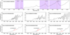 |
Fig. 2 Images of normalized XP spectra of CSTAR_XPM_G. Upper panel shows a standard carbon star with four molecular band ranges marked in purple, and the red dotted line indicating the top of the band head. Middle panel shows three problematic spectra, while the bottom panel presents three spectra with very weak CN773.3 molecular band features. |
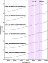 |
Fig. 3 Six representative XP spectra from the 885 objects removed. The two prominent CN bands (purple areas) are located at the 7165–8108 Å and 8160–9367 Å ranges. The red dashed lines mark the top of the band head. The spectra are normalized and offset from one another by k × 1.0 + 0.2 for clarity (where k is an integer that varies from 0 to 6 from the bottom to the top spectrum). |
3 Method
3.1 GaiaNet
Convolutional neural network (CNN; LeCun et al. 1998) is proposed by the concept of perceptual field in biology. By setting several convolution kernels of different sizes, the model can effectively capture a wider range of global and local information, thereby enhancing the feature extraction of the input signal. The neural network model proposed in this work is named “GaiaNet”.
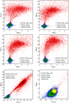 |
Fig. 4 Alternative view from the C2023 sample of the 74 740 CSTAR_XPM_nonG (blue) flagged by ESP-ELS, 8176 selected positive training sample stars (red) from CSTAR_XPM_G, 8556 selected negative training sample stars (green) from CSTAR_XPM_nonG, and 885 deleted stars (yellow). The gray dashed line in the last subplot represents the boundary for the weakest CN strength. |
3.1.1 The structure of GaiaNet
The model is a “light-weight” one-dimensional CNN, an improvement based on the TextCNN model proposed in Kim (2014). The main reason for choosing this algorithm is that the flexible-sized convolution kernel of the 1D CNN can effectively capture and extract detail and overall key features when sliding the convolution in one direction, such a working characteristic makes the model more convincing and interpretable.
There is experimental evidence that extending the depth of a 1D convolutional model can effectively enhance the model’s fitting and feature learning capabilities (Chen 2015). A parallel CNN structure consisting of multiple sets of convolution kernels of different sizes can effectively capture key features of different sizes and achieve similar effects to ensemble learning. We have drawn on these advantages, which are well reflected in the improvement of our model. We first modified the size of the convolution kernel in the input layer so that it can receive one-dimensional data (i.e., data of shape 1 × 343). We added regularization units consisting of batch normalization (BN; Ioffe & Szegedy 2015) and dropout. Both methods are effective in improving the generalization of the model. For the data in each batch, the BN layer first normalizes them. The formula for BN is as follows:
![Mathematical equation: $\[\hat{x}=\frac{x-\mu_B}{\sqrt{\sigma_B^2+\epsilon}},\]$](/articles/aa/full_html/2025/05/aa49619-24/aa49619-24-eq3.png) (3)
(3)
where x denotes the input data, μB and ![Mathematical equation: $\[\sigma_{B}^{2}\]$](/articles/aa/full_html/2025/05/aa49619-24/aa49619-24-eq4.png) are the mean and variance of the data within that batch, respectively, and ϵ is a very small constant to prevent division-by-zero errors. The normalized data are then linearly transformed by a set of learnable parameters (γ and β), which can be optimized by a back-propagation algorithm to obtain the final output, y:
are the mean and variance of the data within that batch, respectively, and ϵ is a very small constant to prevent division-by-zero errors. The normalized data are then linearly transformed by a set of learnable parameters (γ and β), which can be optimized by a back-propagation algorithm to obtain the final output, y:
![Mathematical equation: $\[y=\gamma \hat{x}+\beta.\]$](/articles/aa/full_html/2025/05/aa49619-24/aa49619-24-eq5.png) (4)
(4)
The BN layer avoids drastic changes in the input data distribution caused by parameter updates in the preceding model layer and “pulls” the data back into a stable distribution space. Experimental results indicate that it stabilizes the network, effectively accelerates the training and convergence processes, and enhances the classification accuracy of the model.
Dropout is a commonly used regularization method to avoid overfitting deep network models (Hinton et al. 2012). dropout reduces the risk of model overfitting by randomly discarding the outputs of neurons to reduce the complex dependencies within the network during model training. It is implemented by temporarily erasing the output of a neuron with probability p:
![Mathematical equation: $\[y_i= \begin{cases}\frac{x_i}{1-p}, & \text { with probability } 1-p \\ 0, & \text { with probability } p\end{cases}\]$](/articles/aa/full_html/2025/05/aa49619-24/aa49619-24-eq6.png) (5)
(5)
where xi denotes the original output of neuron i and yi denotes the output of neuron i after dropout. During the training phase, each neuron is randomly selected and turned off with a probability of p and retained with a probability of 1 − p. The retained neuron needs to be scaled by dividing its output value by 1 − p to keep the expectation of the output value constant. We add dropout before the final fully connected layer of the model to prevent overfitting and to improve the model’s generalization.
The 1 × 1 convolution (Lin et al. 2013) can further deepen the network, effectively reduce the number of parameters in the overall convolution layer of the model, enhance the model’s nonlinear fitting ability, allow for flexible dimensioning up and down the feature map, and enable cross-channel information interaction and integration. Global averaging pooling replaces the original practice of stitching the maximum pooled feature maps directly into the fully connected layer. These feature maps are passed through the global average pooling (GAP; Lin et al. 2013) layer and then concatenated to the linear layer to give the corresponding categories. The purpose of this is to share information from the multi-channel feature maps so that they can all contribute to the final result, which is one of the main innovations of this model. The formula is
![Mathematical equation: $\[y_i=\frac{1}{H} \sum_{j=1}^H x_{i, j} \quad i \in[1, n].\]$](/articles/aa/full_html/2025/05/aa49619-24/aa49619-24-eq7.png) (6)
(6)
The GAP is handled with parameters xi,j denotes the feature map value at the j-th row position of the i-th input tensor, and H denotes the height of the tensor. The global averaging pooling calculates the average of all pixel points within a single tensor activation feature map.
We conducted extensive comparative experiments, and the results indicate that balancing the depth and width of the network, combined with the above improvements, can significantly enhance the model’s performance. The flowchart of the model is presented in Fig. A.1 and the overall structure of the model is shown in Fig. A.2.
Sample sets used to validate our algorithm.
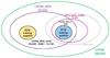 |
Fig. 5 Venn diagram of the relationship of all samples in CSTAR (green frame). Spectra used are from CSTAR_XPM (purple frame, left in the figure). CSTAR_XPM_G is a cross between CSTAR_XPM and golden sample of carbon stars (purplish-red frame, right in the figure), and CSTAR_XPM_nonG is the complement of CSTAR_XPM and CSTAR_XPM_G. Negative sample (yellow) is selected from CSTAR_XPM_nonG, and positive sample (blue) is selected from CSTAR_XPM_G. Gray ellipse frame indicates range of possible carbon stars. |
3.1.2 Important model parameters
The output layer of our model finally passes through a Sigmoid activation function (Lippmann 1987), which is an “S”-type function that converts the real values of the output into a 0–1 probability distribution to represent the confidence level of a positive case. We usually set 0.5 as the threshold value, case greater than the threshold being classified as positive, and case less than or equal to the threshold being classified as negative. It is in line with the 0,1 label defined when we process secondary classification tasks. We used the binary cross-entropy loss (BCELoss; Krogh & Hertz 1991) function to measure the difference between the model output and the true label, which can be interpreted as a maximum likelihood estimate, maximizing the probability of the observed data and finally converging the loss by an optimizer. It is a natural pairing with the Sigmoid activation function when dealing with dichotomous problems, which makes the model output easier to interpret and understand. The formula for calculating the loss of the output from the Sigmoid activation function using BCELoss is
![Mathematical equation: $\[\mathcal{L}=-\frac{1}{N} \sum_{i=1}^N\left[y_i \log \left(\hat{y}_i\right)+\left(1-y_i\right) \log \left(1-\hat{y}_i\right)\right],\]$](/articles/aa/full_html/2025/05/aa49619-24/aa49619-24-eq8.png) (7)
(7)
where N represents the number of input cases in a batch, yi denotes the true label of the ith case, and ![Mathematical equation: $\[\hat{y}_{i}\]$](/articles/aa/full_html/2025/05/aa49619-24/aa49619-24-eq9.png) signifies the predicted probability (model output value) of the ith case. The p-parameter of the dropout layer is also an important parameter, which refers to the proportion of randomly “lost” neurons. The output of our several parallel neural network structures is then spliced together to obtain a vector that is finally discarded with a given p-ratio after the dropout layer. This approach promotes the model’s generalization, effectively avoids model overfitting, and achieves a good integrated learning effect.
signifies the predicted probability (model output value) of the ith case. The p-parameter of the dropout layer is also an important parameter, which refers to the proportion of randomly “lost” neurons. The output of our several parallel neural network structures is then spliced together to obtain a vector that is finally discarded with a given p-ratio after the dropout layer. This approach promotes the model’s generalization, effectively avoids model overfitting, and achieves a good integrated learning effect.
In addition, it is important to balance the size of the convolution kernels. As larger kernels can effectively expand the model’s receptive field and capture features in a broader context, while smaller kernels excel at capturing local details. Therefore, we need to strike a good balance between the whole and the local depending on the actual task.
Furthermore, the batch_size refers to the number of input cases in a batch used to update the model parameters during each iteration. A larger batch_size can speed up convergence by reducing the frequency of parameter updates. Conversely, a smaller batch_size often improves the model’s generalization ability by introducing more variability into each batch, thereby preventing overfitting to the training set. However, the choice of batch_size should be comprehensively considered based on factors such as dataset size, task complexity, memory limitations, and computational resources.
The number of epochs for training is a critical hyperparameter that requires careful consideration. Excessive epochs can lead to overfitting, where the model performs well on the training set with good loss convergence but poorly on the validation set due to decreasing accuracy rates with increasing training epochs. On the other hand, insufficient epochs may result in underfitting, causing the model to inadequately learn key information and perform poorly on the actual test set. Therefore, it is crucial to select an reasonable number of epochs based on factors such as model capacity, data volume, and task complexity.
There are several parameters that play a crucial role in the stochastic gradient descent (SGD) optimization algorithm during the training phase of the model. The lr (learning rate) is a factor that controls the step size of the model weights update, which represents the size of the updated weights at each iteration. A large learning rate may lead to fast convergence of the model during training, but may also lead to the model skipping the optimal solution. A smaller learning rate may result in slower convergence of the model, but it is more likely to achieve a better optimal solution. In our practical tests, we opted for a smaller learning rate to avoid missing the global optimal solution. During the SGD training shown in Fig. 6, the size of each step is fixed, but with the introduction of the momentum learning algorithm, the movement of each step depends not only on the magnitude of the current gradient but also on the accumulation of past velocities. “Momentum” uses historical gradient information to adjust the direction and speed of parameter updates (Polyak 1964), thus accelerating the convergence process of SGD and reducing oscillations during the gradient update process. It can be seen as an inertia introduced to leverage the previous gradient information in parameter updates. The core idea of momentum is to introduce an accumulated gradient history variable, which is similar to momentum in physics and records the direction and velocity of the previous gradient’s motion. During each iteration of the update, the momentum algorithm considers not only the current gradient but also the trends of previous gradients. This allows the parameters to be updated with a certain “momentum” in the direction of the gradient, resulting in faster crossing of flat areas and less invalid oscillation. The parameter update formula in the momentum algorithm is shown below:
![Mathematical equation: $\[v_{t+1}=\mu v_t-\varepsilon \nabla f\left(\theta_t\right),\]$](/articles/aa/full_html/2025/05/aa49619-24/aa49619-24-eq10.png) (8)
(8)
![Mathematical equation: $\[\theta_{t+1}=\theta_t+v_{t+1},\]$](/articles/aa/full_html/2025/05/aa49619-24/aa49619-24-eq11.png) (9)
(9)
where ϵ > 0 represents the learning rate, μ ∈ [0, 1] is the momentum parameter, and f (θt) is the gradient at θt (Sutskever et al. 2013). Our practical tests showed that using this combination of learning rate and momentum parameter significantly improved model accuracy and accelerated the convergence of model loss.
Weight decay is a regularization technique that reduces the complexity of the model by reducing the size of the weights. It applies an L 2 regularization penalty to the weight parameters in the loss function to prevent overfitting so that larger weights are penalized more during training, thus encouraging the model to learn a simpler weight distribution.
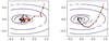 |
Fig. 6 Binary loss function depicted by contour line. The left panel shows the update path of standard SGD, while the right panel shows the path with momentum. The momentum-based update is smoother, more stable, and converges more easily to the global optimum. |
3.2 SHAP
SHAP is an interpretable model based on the game theory principles approach to explain the output of any machine learning model. It connects optimal credit allocation with local explanations using the classic Shapley values from game theory and their related extensions. SHAP can give the extent to which each input feature affects the output of the model and offer a comprehensive and interpretable analysis of the anticipated results of the entire model (Lundberg & Lee 2017). The Shapley value is a concept in game theory that measures the contribution of each player to the cooperative game. In machine learning, different features can be viewed as different “players”, and the combination of their values forms a “cooperative game”. Using the principle of equivalent assignment of Shapley values, we can calculate the contribution or importance of each input feature to the overall model output, and assign a relative contribution score to each feature. In this work, we extend the Shapley value to deep learning models. The prediction value of the model is interpreted as the sum of the importance of each input feature. The relation between the predicted value and importance scores is performed below:
![Mathematical equation: $\[f(x)=g\left(x^{\prime}\right)=\phi_0+\sum_{i=1}^M \phi\left(x_i^{\prime}\right).\]$](/articles/aa/full_html/2025/05/aa49619-24/aa49619-24-eq12.png) (10)
(10)
Specifically, for a deep learning model f : X → Y, where X denotes the input features and Y denotes the class or real value of the output, M is the number of features. The explanation model g(x′) matches the original model f(x) when x = hx(x′), where ϕ0 = f(hx(0)) represents the model output with all simplified inputs toggled off (i.e., missing). SHAP defines the Shapley value for an input xi ∈ X as ![Mathematical equation: $\[\phi(x_{i}^{\prime})\]$](/articles/aa/full_html/2025/05/aa49619-24/aa49619-24-eq13.png) , which represents the marginal contribution of feature xi to the model prediction.
, which represents the marginal contribution of feature xi to the model prediction.
The Shapley value of each feature represents the degree of its influence on the predicted outcome of a single input case. The calculation of the Shapley value is based on combinatorial game theory, which takes into account the interactions between each feature and other features and assigns the final predicted outcome to each feature. For a specific case, the calculation of the Shapley value ![Mathematical equation: $\[\phi(x_{i}^{\prime})\]$](/articles/aa/full_html/2025/05/aa49619-24/aa49619-24-eq14.png) of feature xi is performed below:
of feature xi is performed below:
![Mathematical equation: $\[\phi\left(x_i^{\prime}\right)=\sum_{S \subseteq X \backslash x_i^{\prime}} \frac{|S|!(M-|S|-1)!}{M!}\left[f\left(x_S \cup x_i^{\prime}\right)-f\left(x_S\right)\right],\]$](/articles/aa/full_html/2025/05/aa49619-24/aa49619-24-eq15.png) (11)
(11)
where ![Mathematical equation: $\[S \subseteq X \backslash x_{i}^{\prime}\]$](/articles/aa/full_html/2025/05/aa49619-24/aa49619-24-eq16.png) is any possible subset of all input features excluding
is any possible subset of all input features excluding ![Mathematical equation: $\[x_{i}. f(x_{S} \cup x_{i}^{\prime})\]$](/articles/aa/full_html/2025/05/aa49619-24/aa49619-24-eq17.png) represents the output obtained by adding feature xi to the subset S. f(xS) represents the output obtained by using the subset S for prediction, and the result of subtracting the two values represents the effect of the addition of feature xi on the model output. And the |S|!(M − |S| − 1)! \ M! represents the weight. The overall equation represents the calculated contribution for each feature subset S. This is the contribution from adding feature xi to the feature subset S. Finally, the contribution of each feature subset S is summed to obtain the Shapley value of the feature xi.
represents the output obtained by adding feature xi to the subset S. f(xS) represents the output obtained by using the subset S for prediction, and the result of subtracting the two values represents the effect of the addition of feature xi on the model output. And the |S|!(M − |S| − 1)! \ M! represents the weight. The overall equation represents the calculated contribution for each feature subset S. This is the contribution from adding feature xi to the feature subset S. Finally, the contribution of each feature subset S is summed to obtain the Shapley value of the feature xi.
This method allows us to compare the Shapley values of different features to determine how much they affect the output of the model. It has been flexibly applied to various deep learning models, including CNNs, recurrent neural networks (Werbos 1988), and others. We use the SHAP in our model to interpret the key features that affect the model output. In addition, SHAP provides several visualization tools and methods that helped us understand the model better.
3.3 Evaluation index
In addition to the accuracy criterion, we also introduce other evaluation metrics such as recall and precision to effectively measure the model’s data mining performance during dataset validation. We define TP (true positive) as the number of cases whose categories are true and predicted categories are also positive, FN (false negative) as the number of cases whose categories are true but predicted categories are negative, FP (false positive) as the number of cases whose categories are false but predicted categories are positive, and TN (true negative) as the number of cases whose categories are false and predicted categories are also negative.
Accuracy refers to the proportion of the number of accurate cases classified by all categories to the total number of cases. We calculated it as
![Mathematical equation: $\[Accuracy=\frac{T P+T N}{T P+T N+F P+F N}.\]$](/articles/aa/full_html/2025/05/aa49619-24/aa49619-24-eq18.png) (12)
(12)
Precision refers to the proportion of the number of correctly predicted positive cases to the total number of predicted positive cases. It is calculated as
![Mathematical equation: $\[Precision=\frac{T P}{T P+F P}.\]$](/articles/aa/full_html/2025/05/aa49619-24/aa49619-24-eq19.png) (13)
(13)
Recall refers to the proportion of correctly predicted positive cases relative to all actual positive cases. It is calculated as
![Mathematical equation: $\[Recall=\frac{T P}{T P+F N}.\]$](/articles/aa/full_html/2025/05/aa49619-24/aa49619-24-eq20.png) (14)
(14)
We also used a confusion matrix to be able to see the performance of the model more intuitively, as it effectively illustrates the distribution across different classes. For our carbon star data mining work, the idea is to have as many TP cases as possible and as few FN cases as possible (i.e., as large a recall rate as possible), so we used this as our main validation set diagnostic.
3.4 Resampling technique
The resampling technique (Efron 1979) is an important data processing method used to solve the problem of imbalance in the categories of a dataset. For example, when the number of positive cases is slightly less than the number of negative cases, resampling techniques can be used to increase the number of positive cases. This is done by randomly copying or generating new positive cases, thus making the number of positive and negative cases consistent and balanced. This can effectively prevent the models from “collapsing” into categories with large case sizes during training.
4 Results
After validation with several sets of parameters in Sect. 3.1.2, we fixed the training parameters of the model as follows: p = 0.4, lr = 0.005, momentum = 0.9, weight_decay = 0.001.
4.1 Analysis and experiments on the dataset
Almost all N-type carbon stars are in the AGB evolution stage, where the carbon abundances in their atmosphere were produced in the stellar interiors, and were brought to the surface by the TDU process. Almost all of them are intrinsic, thermally pulsing AGB stars (i.e., TP-AGB stars with large luminosities; Abia et al. 2002). This kind of carbon star typically exhibit stronger C2 and CN molecular bands than usual stars with temperatures below 3800 K (Gaia Collaboration 2023). Of course, there are also some kinds of carbon stars with relatively high surface temperatures, whose spectral types can be K or even G, and they are often extrinsic carbon stars. However, there is a large number of giant stars with the spectral type G, K, and M, which have similar colors, surface temperatures, and luminosities to the carbon stars, making it impossible to distinguish between the carbon stars and other giants just from the HR diagrams, but now possible through Gaia’s spectroscopy. Lebzelter et al. (2023) and Sanders & Matsunaga (2023) have demonstrated its potential for separating C-rich and O-rich stars.
We found that almost all of the CSTAR_XPM_nonG are M giants through the GBP − GRP and log g diagram (see Fig. 1), and their distribution overlaps with the region where the golden carbon stars located. To obtain reliable luminosity and color parameters, we corrected the photometric data with 3D interstellar extinction (Green et al. 2019), and then a color-magnitude diagram is shown in Fig. 7.
After the extinction correction, we calculate the absolute magnitudes (MG)0 and the intrinsic color index of (GBP − GRP)0 for 4002 positive sample stars, 6761 negative sample stars, and 64761 stars of CSTAR_XPM sample, respectively. Most of the CSTAR_XPM stars have 1 < (GBP − GRP)0 < 3 and (MG)0 < 2 mag, and most of the carbon stars have 2 < (GBP − GRP)0 < 4 and (MG)0 < −1 mag. This suggests that the CSTAR_XPM_G sample may consist mostly of brighter and cooler N-type carbon stars. From the corrected color-magnitude diagram, we also found that about half of the negative sample stars have a (GBP − GRP)0 ≥ 1.6, while the (GBP − GRP)0 of M giants should usually be larger than 1.6. We estimated that there are about half of the G and K giants in the CSTAR_XPM_nonG, which is corroborated by our later cross-matched results with the LAMOST DR10 spectroscopic data in Sect. 5.1. Hence, the CSTAR sample also includes a large mixture of other types of stars, rather than overwhelmingly M stars. In addition, a portion of the CSTAR_XPM_G has (GBP − GRP)0 < 2 and relatively lower luminosities. If these sources are located in the crowded regions of the Galactic plane where the dust distribution is complex and non-uniform, the true interstellar medium does not follow a simple Gaussian process (Green et al. 2019). In this case, their extinction must be treated with caution. If their color index estimates are correct, as suggested by Fig. 11 of Li et al. (2024), they are most likely extrinsic warm carbon stars with spectral types of G- or K-like Ba stars. It can be seen that there is a slightly clearer distinction between positive sample and negative sample in the color magnitudes, but some of the stars are still mixed together. However, elemental abundances are also reflected in the spectra (Abia et al. 2002). Specifically, the carbon stars are characterized by the strong absorption lines of carbon molecules in their spectra. This offers the possibility of a spectroscopic data-driven approach to distinguish the two directly from the stellar spectra. C2023 proposed screening carbon stars by R773.3 and R895.0, it could be partially contaminating and would result in the loss of some potential carbon stars through our inspection.
As mentioned in Sect. 2.2, we carefully selected a negative sample of 8556 spectra from CSTAR_XPM_nonG and a positive sample of 8176 spectra from CSTAR_XPM_G. We equalized the number of positive and negative samples by randomly adding positive spectra using the resampling techniques. Thus, we constructed a training dataset through careful visual inspection and machine ranking to ensure better distinction for deep learning and provide meaningful, interpretable analysis.
4.1.1 Model validation
We randomly selected 70% of the datasets to train the classification model, and the remaining 30% was used as the validation set to measure the model’s performance as the epochs increased.
The best performance of the model occurs when the epochs are 9, 16, 17, 18, and 19. The final recall rate in the validation dataset is 100%, the accuracy is also 100%. The confusion matrix is shown in Fig. 8, showing that our model has extremely high accuracy and reliability for classifying all stars in the validation dataset. Our model can easily distinguish the spectra of cold and bright carbon stars with strong carbon molecular bands from the spectra of giant stars of G, K, M types. We provide the necessary comparisons and explanations in Sect. 4.2.
We also plot the change in the correctness of the training and validation sets and the number of FP, and FN spectra as the training epochs increase, as shown in Fig. 9. The best performance on the validation set (30%) is 100% accurate, with excellent convergence and no overfitting of the model.
 |
Fig. 7 Distribution of CSTAR_XPM and the training sample on (MG)0 versus the (GBP − GRP)0 diagram. All the samples have been corrected for 3D extinction. Panel a: Distribution of the CSTAR sample. Panel b: Distribution of the training sample. Panel c: Distribution of carbon stars from the training sample. Panel d: Distribution of non-carbon stars from the training sample. |
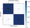 |
Fig. 8 Confusion matrix of our model predicted on the validation set. Label 0 represents a non-carbon star, and label 1 represents a carbon star. |
4.1.2 Comparison with other algorithms
In the past decades, many machine learning includes integrated learning methods (KNN: Cover & Hart 1967; SVM: Cortes & Vapnik 1995; RF: Breiman 2001; XGBoost: Chen & Guestrin 2016, etc.) have been successfully applied to stellar spectral classification and physical parameter estimation. In contrast, CNNs are well known to have been used with great success in the field of image recognition, so we see the potential for the use of one-dimensional convolutional deep learning networks in spectral recognition.
In Table 3, we compiled a comparison of the accuracy (%), recall, and error rate (%) of several common machine learning classification models with our model on the performance of the validation set.
Recall is a very important evaluation index that effectively measures the rate of retaining positive sample. Our model retains all stars of positive sample and demonstrates approximately a 0.43% improvement over other algorithms, resulting in an overall accuracy increase of about 0.3%. The reason for the error rate of 0 in the validation set is likely to be the excellent overall architecture of our model, which is mainly reflected in the natural advantages of the convolutional model in feature extraction, as well as some necessary innovative improvements. On the other hand, we have conducted “expert” screening and purification of the training data to exclude erroneous spectra and ensure the high purity and reliability of the training data, combined with some necessary data enhancement methods to ensure that the model can learn the appropriate information. Though of course, The spectra of positive sample exhibit strong CN molecular bands, making them easily distinguishable from negative sample.
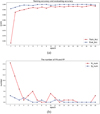 |
Fig. 9 GaiaNet’s performance with the change of epoch numbers. Panel a: accuracy of the model on the training set (red) and validation set (blue); Panel b: number of misclassified spectra of the model on the validation set. |
Models’ performance on a 30% validation set.
4.2 Model interpretation and key features
As an extension of the Shapley value in machine learning, SHAP value is used to quantify the effect of features on our model’s output (i.e., the confidence of a carbon star as mentioned in Sect. 3.1.2). We consider each wavelength in a spectrum as a feature, and the corresponding flux to each wavelength as the feature value. The SHAP model can explain the model output by calculating a SHAP value for each feature of a given spectrum, which indicates the importance impact or contribution of the feature to the model output. A positive SHAP value indicates that the feature contributes positively to the model’s prediction of the spectrum being a carbon star, while a negative value means it contributes negatively. The larger the absolute SHAP value, the greater the impact of the feature on the model output. For a spectrum, the sum of SHAP values of each feature can be used to approximate the output of the classification model. We can also calculate the distribution of the most important features based on the statistics of SHAP values from a large sample.
To get an overview of which features are most important and intuitively understand the influence of them on the model prediction results, we randomly selected 1024 carbon stars of positive sample and 1024 non-carbon stars of negative sample as background spectra of the deep explainer interpreter of SHAP, calculated the SHAP values of these spectra, and plotted in Fig. 10. The top 30 most important features were shown in this beeswarm plot, which were ranking by the sum of absolute SHAP value magnitudes of them over all 2048 spectra, and uses SHAP values to show the distribution of the impacts each feature has on the model output. For a particular feature, SHAP first normalizes its values across all spectra, and the normalized feature values are then mapped onto a color gradient bar. The feature point is assigned different colors from blue to red. The color blue represents a feature point value that is relatively small, and red means that a feature point value is relatively large.
Therefore, the beeswarm plot provides an intuitive reflection of how the feature influences the output results for different values, visualizing the link between feature values and model interpretation. As shown in the figure, we can see that the wavelength range 8900–9000 Å is the location of the peak arising from the molecular band head. The larger the values of these feature points are, the more positively the model predicts carbon stars. Near 8100 Å and 9300 Å are the locations of the troughs arising from CN molecular absorption bands. The smaller these feature values are, the more positively the model predicts carbon stars. It is evident that the most striking distinguishing feature is the presence of these two troughs.
To better illustrate the differences in key feature contributions within a single spectrum, the background spectrum for calculating SHAP values can be chosen as the smooth pseudo-continuum after polynomial fitting using the approach of Zhang et al. (2021). It serves as a baseline and reference for individually calculating the SHAP value of each feature in each spectrum. Contrasting with such a baseline allows for a clearer identification of the trough and peak features in each spectrum. Subsequently, we can generate an intuitive and clear feature distribution heatmap for given spectrum shown in Fig. 11, which facilitates the easy location of the key spectral features concerned by our model.
However, if we want to get a more statistically significant and reach a quantified conclusion, we need statistical information on the SHAP values of a large enough sample. For this purpose, we calculate the average SHAP values of each feature for all positive and negative samples. As shown in Fig. 12, the interpretation ranges of positive features for the positive sample are consistent with the CN features. It is mainly distributed in the ranges 9140–9440 Å, 7900–8360 Å, 8820–9060 Å, and 7600–7820 Å, showing that relatively large SHAP values were assigned to both peak and trough ranges in the CN molecular bands. However, compared with the positive carbon star sample, the average SHAP values in these regions of the negative sample are much smaller. In addition, the negative sample showed a very strong negative contribution in the range 8420–8900 Å, which is the most significant distinguishing feature of this sample. We note that the average SHAP values of the positive sample is also negative in the 8420–8620 Å region. We suspect that this is related to the absorption feature of Ca II (8484–8662 Å), which is considered by the model to be a negative feature. We can see that the location of the model’s main concern is the strong CN molecular band feature at the red end of the spectrum, which is consistent with the actual interpretation in Sect. 5.3. Next, we showcase these key features.
The sum of SHAP values in Fig. 12 represents the sum of the average SHAP values across the feature dimensions of positive or negative sample. For the positive sample, the sum of SHAP values is 0.99894. We summarize the main feature regions of the golden sample of carbon stars, which serves as the basis for our subsequent identification work. We calculated the sum of SHAP values over five main intervals listed in Table 4. Among them, the range 6780–7460 Å includes the peak characteristic of 6780–6920 Å and the absorption trough characteristic of 7000–7460 Å.
The reason our model only identifies the prominent CN features in the red end of the positive sample spectra, while almost failing to detect the C2 features in the blue end, can be attributed to two factors. Firstly, the flux values in the blue end are too small relative to the entire spectrum, making the C2 features much less significant compared to the prominent CN features. Secondly, C2023 filtered golden sample carbon stars in relatively cold (most of them have GBP − GRP > 2; Gaia Collaboration 2023) CSTAR sample based on the prominent CN features rather than the much weaker C2 features. This results in more than half of the targets in the golden sample of carbon stars having almost no C2 features.
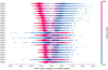 |
Fig. 10 Contribution ranking of features to the model result based on SHAP values. Each point represents a feature from the spectrum. The horizontal axis shows the SHAP values, while the vertical axis ranks the top 30 spectral features for identifying carbon stars, from most to least important. The color of each point indicates the size of the feature value. |
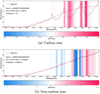 |
Fig. 11 Feature heatmaps for individual spectral interpretations. The baseline is a background pseudo-continuum used to compute SHAP values, highlighting spectral features. The color indicates the SHAP value size: redder features contribute positively, while bluer ones contribute negatively to the model’s interpretation of carbon stars. The sum of SHAP values approximates the model output, with a larger sum indicating a stronger likelihood of the spectrum being identified as a carbon star. |
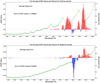 |
Fig. 12 Average SHAP values per feature with a 20 Å wavelength bin size. Red and blue indicate positive and negative SHAP values, respectively. For comparison, the average spectra of positive and negative samples are overlaid as green scatter points. The upper panel highlights the two prominent CN bands with gray shading. |
Wavelength range and SHAP value score of the five most important features from the positive sample.
4.3 451 new carbon star candidates
We combined the model training and validation accuracy, as well as the changes in FP and FN in Sect. 4.1.1, and ultimately determined the training epoch number of the model as 16. We applied the model trained based on the dataset provided in Sect. 2.2 to the 74 740 stars of CSTAR_XPM_nonG, and 451 new carbon star candidates were obtained. The spectra of these stars exhibit relatively prominent CN molecular bands compared to typical giant stars but are weaker than most golden sample stars. Their spectra show reduced flux at the blue end and hardly any significant C2 features are visible. In Fig. 13 we show some spectra of these stars.
The color-magnitude diagram and distribution position of the CN band head strengths are shown in Fig. 14. The colormagnitude map shows that our new carbon star candidates occupy the location of the carbon star golden sample but mainly concentrate in the hotter regions. From the strength map, our new carbon star candidates mainly occupy the position of weak CN band carbon stars mentioned in C2023.
The spatial distribution of the candidates is shown in Fig. 15. Since the positive sample comes from the golden sample of carbon stars, they are distributed throughout the Galactic disk, the LMC, and the SMC. However, these new candidates are primarily distributed in the dense Galactic inner disk, an area characterized by substantial amounts of interstellar dust that contribute to increased extinction. Consequently, the observed degradation of their spectral shape, particularly at the blue end, is likely caused by a lower S/N or observation in crowded and highly reddened sky regions (Lebzelter et al. 2023). This also explains why many of them became hotter ((GBP − GRP)0 < 2) after 3D extinction correction (Green et al. 2019). If their color index estimates are correct, similar to the study of C-rich stars in the Milky Way’s bar-bulge (Sanders & Matsunaga 2023), these stars are likely to be the result of binary evolution. However, the possibility of single star evolution cannot be ruled out due to the possible extinction errors.
After cross-matching our 451 new carbon star candidates with LAMOST DR10, four common sources were obtained, two of which were labeled as carbon stars by LAMOST’s pipeline (Wei et al. 2014). Cross-matching with SIMBAD yielded 73 common sources, 28 of which were labeled as C* in the main_type or other_types attribute.
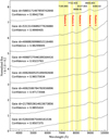 |
Fig. 13 XP spectra of eight candidate carbon stars similar to the normalization manner in Fig. 3. The yellow areas highlight key features we summarized. The blue dashed line marks the position of CN troughs, and the red indicates the peaks. |
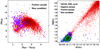 |
Fig. 14 Color-magnitude diagram (dereddened) of the new candidates (shown on the left) and the molecular band head strength of the new candidates (shown on the right). |
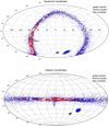 |
Fig. 15 Spatial distributions of our results drawn in equatorial and Galactic coordinates. The gray spots denote the 15 400 golden sample of carbon stars. The blue spots represent the 8176 positive sample from CSTAR_XPM_G. The red spots are the 451 new carbon star candidates from CSTAR_XPM_nonG. |
5 Discussion and analysis
Following Wallace (1962), we plot all the CN absorption line positions as dotted lines at the red end of the spectrum in Figs. B.1 and B.2.
5.1 Cross-match with LAMOST DR10
We cross-matched the RA and Dec of all the 83028 CSTAR_XPM sample stars with the catalog of low-resolution spectra from LAMOST DR10, to obtain the subclass types given by the LAMOST’s pipeline (Wei et al. 2014). There are 442 sources labeled as carbon stars, and 1131 are not. Among the sources not labeled as carbon stars, there are 351 G-type stars (31%), 232 K-type stars (20.5%), and 509 M-type stars (45%), the vast majority of them come from CSTAR_XPM_nonG.
To better understand the formation of characteristic troughs in the Gaia XP spectra of carbon stars, the LAMOST spectrum of the same source was drawn in Fig. B.1 to determine the CN absorption position. Using the fast Fourier transform and interpolation method of Zhang et al. (2021), the LAMOST spectrum was convolved to the resolution of the approximate Gaia XP spectra to show the difference in the absorption region under different resolutions. We also plotted the same figures for common sources of G-, K-, and M-type stars as a comparison to illustrate the areas of feature differentiation.
We found that the most significant feature shared by the negative sample of G-, K-, and M-type stars compared with the positive sample of carbon stars is the Ca II line absorption feature in the range of 8484–8662 Å (Li et al. 2023), which can also be identified in the Gaia XP spectra. When the temperature is low, near the M type, the prominent TiO5 (7126–7135 Å; Li et al. 2023) and K I (7664.9–7699.0 Å; Lépine et al. 2003) absorption line features are prominent and also visible in the LAMOST and Gaia XP spectra after resolution reduction. During the change of spectral type from M to G, the absorption characteristics of TiO5 and KI gradually weaken in the spectra until they almost disappear. This trend is consistent with the gradual approach of the negative shape values at TiO 5 and KI towards zero in Fig. 16. However, carbon stars exhibit broader and deeper CN absorption features at 6900–7300 Å, and 7900–8300 Å, and a set of three peak tops at 6830 Å, 7780 Å, and 9000 Å (Sanders & Matsunaga 2023). While M-type non-carbon stars also display peak structures, such as the peak tops at 7050 Å and 7600 Å, their positions are entirely different. Therefore, both the characteristic peaks and troughs in the spectra of carbon stars are crucial distinguishing features from other types of stars.
From Fig. 16 we calculate SHAP values for the obtained G-, K-, and M-type stellar spectra separately and then statistically. we can see that the absorption characteristics near 8300 Å and 9400 Å are gradually enhanced and the sum of SHAP values increases with temperature increase. Therefore, we hypothesize that in the CSTAR_XPM_nonG-, G-, and K-type stars are more likely to be carbon star candidates. After a visual inspection of the 1131 stars, we estimate that G stars may contain 10% candidates and K-type stars may contain 2.6% candidates. The reason is that if a low-temperature star has a high C abundance, its redend molecular band characteristics will be more obvious. It will be easier to select by the method of C2023. On the contrary, if at high-temperature conditions, the carbon molecular band characteristics would be relatively weak. In other words, if a source can still show the carbon characteristics at high temperatures, its C abundance can be considerable.
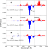 |
Fig. 16 Average distribution of SHAP values per feature for the G, K, and M types. The wavelength range is intercepted from 6500 to 10 000 Å. |
5.2 Comparison with the results of Sanders & Matsunaga (2023)
Lebzelter et al. (2023) released a candidate catalog of 1 720 588 long-period variables (LPVs). After cross-matching with Gaia DR3 data, we found that there are 13 513 stars in the golden sample of carbon stars and only 1289 stars in CSTAR_XPM_nonG are classified as LPVs. Based on the UMAP unsupervised algorithm, Sanders & Matsunaga (2023) have presented 23737 C-rich candidates from the LPV candidate catalog above. There are 40 of the above 1289 LPVs in the list of our 451 new carbon star candidates, and 26 are also identified as C-rich stars by Sanders & Matsunaga (2023). There are 20 common objects between our above 40 candidates and 26 C-rich stars of Sanders & Matsunaga (2023), where six objects are not included in our results. We show the heatmaps of these six objects in Fig. D.1.
The majority of the golden sample carbon stars are TP-AGB stars, typical of long-period variable stars, so it is not surprising that they are overwhelmingly classified as LPVs by Sanders & Matsunaga (2023). However, the proportion of CSTAR_XPM_nonG stars labeled as LPV candidates is quite small. This may be attributed, to their low S/N ratio, a relative lack of data points in the Gaia G time series, small variability amplitudes, or short periods. This would lead to their nondetection as period signals by the SOS module of Lebzelter et al. (2023). On the other hand, they have not yet evolved to the TP-AGB phase with periodic variability, which is consistent with their location site on the HR diagram (Fig. 7). Regarding why only a few dozen of the 1289 LPVs in the CSTAR_XPM_nonG are classified as C-rich stars, this is likely due to selection effects. In CSTAR_XPM, the majority of C-rich LPVs were selected by the algorithm of C2023 and included in the golden sample, resulting in the remaining 1289 stars being predominantly O-rich LPVs, as well as some C-rich LPVs with weak carbon spectral features that were not detected by the algorithm. Therefore, mining possible carbon stars from CSTAR_XPM_nonG is not a simple task. Our candidates contain the vast majority of C-rich stars identified by Sanders & Matsunaga (2023), which demonstrates the high completeness of our method. The other six stars are significantly different from the golden sample, but there is no denying that they still are possible carbon stars. Our model scores them with a not-low confidence level, just not above the 0.5 threshold (see Sect. 3.1.2). Although the positive sample our model learned is from the golden sample of carbon stars with strong molecular bands, it is still able to identify quite a few carbon stars exhibiting relatively weak CN molecular band features. This demonstrates the good generalization ability of our model and encourages future systematic exploration of carbon stars across all of Gaia’s XP spectra.
5.3 Explanation of key features
The position of the CN absorption lines with a wavelength greater than 6900 Å in the literature (Wallace 1962) are marked in Fig. B.2.
From the figure, we can see that there are some differences in the shape of the molecular absorption band regions in the spectrum at different resolutions. The continuous and dense CN absorption line region in the LAMOST spectrum shows the form of wide and deep CN characteristic troughs in the Gaia spectrum, such as Feature 5 and Feature 2. We posit that this is the combined absorption effect of superimposed multiple molecular absorption lines in the spectrum at Gaia spectral resolution, we call it the “mixed-molecular-absorption-band” in the Gaia spectrum. It can be seen that Feature 1 and Feature 2 are consistent with the dense CN absorption line regions, except for the small SHAP value assigned by the absorption region of Feature 5, which may be caused by the weaker signal flux values in the spectra compared to Feature 1 and Feature 2.
As for the peaks observed in the spectra, they are a reflection of the relative decrease of opacity. When the molecular absorption on both sides of the peak becomes stronger, it will increase opacity and thus form the characteristic trough. Consequently, the region with less opacity stands out as a peak in the spectrum. Hence, the characteristic peaks of Feature 3 and Feature 4 in the shadow region are are also meaningful for distinguishing the positive and negative samples.
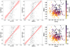 |
Fig. 17 Relationship between band head strengths and confidence level, and with the sum of SHAP values. |
5.4 Reliability analysis of new candidates
To verify the reliability of the new candidates, we mainly analyzed the relationship between the molecular band head strengths (R773.3 and R895.0) and the confidence levels, as well as the relationship between the strengths and the sum of SHAP values. We also calculated the average sum of SHAP values for the new candidates in Fig. C.1.
From Fig. 17, it is clear that there is an approximately linear relationship between the strengths and the confidence, SHAP value given by the models. Moreover, it is evident that smaller values of R773.3 and R895.0 correspond to lower confidence and SHAP values from the color-coded scatter plots. Conversely, as the values of R773.3 and R895.0 increase, so do their confidence and SHAP scores (dark color). Such strong positive correlations prove that our candidates should be reliable.
5.5 Origins of the new carbon star candidates
Since the absolute magnitudes of our new carbon star candidates are all less than three, according to the dividing line at (MG)0 = 5.0 mag between carbon dwarfs and carbon giants proposed by Li et al. (2024), we have selected carbon giants. Additionally, only 40 of these candidates have been reported as LPV candidates by Lebzelter et al. (2023). This implies that many of them might not have evolved to the TP-AGB phase with intense TDU episodes, or alternatively, they could be TP-AGB stars but whose S/N ratio or observed amplitudes are insufficient for detection by the algorithm. The smaller amplitudes might not only be related to the evolutionary state of the stars but could also be influenced by observations in crowded regions, where the light curves of variable stars may be compressed, leading to measured amplitudes smaller than their true values (Lebzelter et al. 2023), and potentially resulting in a poor S/N ratio.
Extinction correction in crowded and highly reddened sky regions must be treated with caution. If the color index corrections for the candidates are accurate, their bluer colors ((GBP − GRP)0 < 2) compared to the positive sample likely indicate that they are extrinsic carbon stars (products of binary evolution). Nevertheless, it cannot be excluded that some of these stars are in the TP-AGB phase. Their weaker carbon spectral features may result from temperature and metallicity effects. A higher temperature promotes the dissociation of carbon-bearing molecules in stellar atmosphere, while a higher metallicity can directly influence the C/O ratio, which determines the global spectral shape of carbon stars (Abia et al. 2002). Additionally, they might be newly formed carbon stars that have undergone limited evolution (hence warmer) with a few thermal pulses (TPs). Fewer TDU episodes imply that the dredged-up carbon in their atmospheres remains at relatively low levels but is already sufficient to establish a C/O ratio larger than unity (Abia et al. 2002; Herwig 2005). In contrast to the evolved N-type carbon stars (C/O ratio significantly exceeding unity), that have a more pronounced mass loss (Vassiliadis & Wood 1993) and become optically obscured due to dust formation, these “young” carbon stars appear to be more valuable for abundance analysis (Abia et al. 2002). Furthermore, the limited amount of dredged-up carbon could also be due to the weak TDU strength in low-mass stars (Sanders & Matsunaga 2023). Finally, it is worth noting that their weak spectral carbon features may also be attributed to the lower S/N ratio or to observations in crowded or highly reddened sky regions, rather than a genuinely low carbon abundance in their atmospheres.
6 Conclusions
In this work, we have demonstrated the capability of the proposed GaiaNet model in classifying carbon stars within the CSTAR_XPM sample. Additionally, we have provided compelling feature attributional interpretations for the model’s outputs using the SHAP method. This “magic” empowers the originally incomprehensible black-box model with the ability to proactively “speak up” and make its discriminations traceable. Our main results and conclusions are as follows:
- (i)
The method presented in C2023 for calculating the strength of molecular bands has proven effective in selecting carbon stars with strong CN features. However, it lacks effectiveness in identifying hotter carbon stars with weaker CN features and may introduce contamination. In contrast, the proposed GaiaNet model demonstrates a superior capability in robustly distinguishing between carbon and non-carbon stars from the training datasets. In particular, it is able to identify carbon stars with weak CN features from CSTAR_XPM_nonG. Compared to four conventional machine learning methods, the GaiaNet model exhibits an average accuracy improvement of approximately 0.3% on the validation set, with the highest accuracy reaching up to 100%. The flexible parameter architecture provides the model with an enhanced fitting capability and stability through the incorporation of operations such as 1 × 1 convolution, GAP, BN, and dropout layers. Furthermore, optimized training methods, including momentum and weight decay, were employed. By utilizing deep learning models with varying convolution kernels during the 1D convolution process, the GaiaNet model effectively captures both local and global features from low-resolution smoothed spectra. Coupled with the nonlinear capabilities provided by an appropriate model’s depth, the model possesses natural advantages in handling Gaia’s XP spectra;
- (ii)
We utilized SHAP for feature attributional interpretation with the GaiaNet classification model based on a positive sample. We presented clear feature heatmaps for each spectrum, which serve as a basis for judgment and identification of each spectrum. Based on the statistical analysis of SHAP values from the spectra, we found that the C2 features provide only a weak signal at the blue end of low flux values and have a minimal presence in many cold carbon stars. Therefore, they were not selected by our model. We summarized five key spectral feature regions: 6780–7460 Å, 7600–7820 Å, 7900–8360 Å, 8820–9060 Å, and 9140–9560 Å. Among them, the 7900–8360 Å and 9140–9560 Å regions are the most obvious trough areas. These two regions contribute over 80% of the SHAP value due to CN molecular absorption. The 7600–7820 Å and 8820–9060 Å regions contribute about 16% and are also important distinguishing features due to the peak areas from the strong CN molecular absorption on both sides. The 6780–7460 Å region contains relatively weak peaks and troughs, making the smallest contribution (less than 4%). We hypothesize that this is related to the spectral values, which seem to be addressable through improved spectral normalization methods. These results suggest that our model can effectively learn and capture the key distinguishing features that are consistent with CN molecular absorption lines and visual identifications by astronomers in the classification of carbon star spectra. These five key feature regions will be essential for future systematic mining of carbon stars from Gaia’s XP spectra;
- (iii)
We identified 451 new carbon star candidates from CSTAR_XPM_nonG using the trained classification model. Compared to the band head strength calculation method, our approach effectively detects more carbon star candidates that have weaker CN features than those found in the golden sample of carbon stars. These candidates align with the weak CN feature carbon stars depicted in Fig. 21 of C2023. The weaker CN features might be a function of temperature and metallicity effects because many of these stars become bluer according to their corrected colors ((GBP − GRP)0 < 2), and they show stronger negative contributions caused by Ca II absorption features near 8500 Å A based on the statistical analysis of SHAP values compared to the positive sample. Moreover, most of them are not classified as LPVs by Lebzelter et al. (2023), indicating that they could be extrinsic carbon stars. However, the possibility that they are AGB carbon stars with less evolution (limited TPs or mild TDU events) cannot be ruled out. Their observed weak carbon spectral features may suggest a small amount of dredged-up carbon, with the C/O ratio not significantly larger than one. However, caution must be taken when analyzing these candidates, as they are mainly located in the crowded region of Galactic inner disk;
- (iv)
We cross-matched the 451 new candidates with LAMOST DR10, resulting in a total of four common sources. Among them, two were identified as carbon stars by the LAMOST 1D pipeline. By cross-matching with the SIMBAD database, we obtained 73 common sources. Among these, 28 had already been reported as carbon stars or carbon star candidates in previous work. To compare the results in Sanders & Matsunaga (2023), we constructed a reference sample containing 1289 LPVs. In this work, we have discovered 40 potential carbon stars from the 1289 LPVs, and they identified 26 C-rich stars, which includes only six stars that are not among our candidates. This is due to the significantly different spectral features of the six stars from the positive sample, which results in their confidence being lower than 0.5. Furthermore, the assigned confidence and SHAP values for each spectrum were used to quantify the model’s output, revealing a strong correlation with the band head strengths of R773.3 and R895.0. This suggests that the classification model primarily focuses on the crucial CN features, and the learned features make sense. Hence, our model can efficiently learn the key features between carbon and non-carbon stars in the CSTAR_XPM sample, and the model’s reliability is further validated.
Due to the limited diversity of the positive training sample, there are still some carbon stars with weaker CN features that are not recognized by our algorithm. Their probabilities given by the model’s output do not exceed the threshold of 0.5 but are significantly larger than zero. Thus, the proportion of candidates in CSTAR_XPM_nonG could be higher, especially for the G- and K-type stars, which is predictable if a lower threshold is set. We roughly estimate that the loss percentage is at least about 5%. In future work, it will be feasible to make reasonable improvements to the classification model and incorporate more carbon stars with weaker CN bands into the positive sample in order to search for and identify more potential warm candidates from CSTAR. The algorithm will then be able to be expanded to the entire Gaia XP spectral dataset, thereby significantly enriching the number of known carbon stars. Indeed it would be interesting to perform further classification and meaningful analysis. Given the resolution of Gaia’s XP spectra, our method can be directly transferred to the upcoming China Space Station Telescope, especially for the interpretation of different types of stars whose spectral properties are still unclear.
Data availability
To exploit these samples, the identification results of “CSTAR” are saved in the spectraltype_esphs field of the astrophysical_parameters table. The list of source_id for golden sample of carbon stars is available in the gold_sample_carbon_stars archive of the performance verification table. All of the above data can be retrieved in Gaia archive.
Tables of 451 new carbon star candidates are available in electronic form at the CDS via anonymous ftp to cdsarc.u-strasbg.fr (130.79.128.5) or via http://cdsweb.u-strasbg.fr/cgi-bin/qcat?J/A+A/697/A107.
Acknowledgements
We would like to thank an anonymous referee and editors for their helpful comments and suggestions. We thank Bo Zhang for his effective spectral smoothing method and helpful discussions. We thank Xiao Kong for his help with the data. This study is supported by the National Natural Science Foundation of China (NSFC) under grant Nos. 12173013, 12273078, and U1931209; the National Key Basic R&D Program of China (No. 2019YFA0405500); the project of Hebei provincial department of science and technology under the grant number 226Z7604G, and the Hebei NSF (No. A2021205006). W.Y. thanks the science research grants from the China Manned Space Project, and we also acknowledge the grants from the China Manned Space Project under Nos. CMS-CSST-2021-A10. This work has made use of data from the European Space Agency (ESA) mission Gaia (https://www.cosmos.esa.int/gaia), processed by the Gaia Data Processing and Analysis Consortium (DPAC; https://www.cosmos.esa.int/web/gaia/dpac/consortium). This research has used the SIMBAD database, operated at CDS, Strasbourg, France. This research also used the low-resolution spectral data of LAMOST DR10 (the Large Sky Area Multi-Object Fiber Spectroscopic Telescope DATA RELEASE 10; https://www.lamost.org/dr10/v1.0). LAMOST is operated and managed by the National Astronomical Observatories, Chinese Academy of Sciences.
Appendix A Model structure
A.1 The flowchart of GaiaNet
Figure A.1 shows the overall flow of GaiaNet. Our model is made up of 16 parallel network structures, each with different-sized convolutional input layers to be able to capture and extract key features in different fields of view. The same deep hidden layer network structure is then used, which consists of three convolutional layers, two pooling layers, a maximum pooling layer, and a average pooling layer. The deeper hidden layer structure helps enhance the model’s nonlinear fitting capability, allowing for the extraction of key nonlinear features. The overall architecture of the model is derived from “textCNN,” which has been improved by several iterations. We referenced the NIN network by introducing a 1×1 convolution, and a GAP operation (Lin et al. 2013). The Inception Module network structure from GoogLeNet was borrowed, that is, a structure consisting of multiple parallel and smaller dense convolutions with pooling approximating sparse connections (Szegedy et al. 2015).
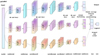 |
Fig. A.1 Overall flowchart of GaiaNet. Convolution kernels of different sizes are used to extract features from different receptive field sizes. The arrows indicate the tensors of feature maps after convolution, pooling, or linear operations. A global max-pooling layer downsamples the feature map to compress its size and captures the most sensitive features. These are then combined into a tensor, which then undergoes GAP to share each feature value across the entire feature map. The resulting tensor is passed through a fully connected layer, which summarizes the features to produce a high-level abstract representation. Finally, a Sigmoid layer converts the neural network’s output into a probability distribution, making the predictions easier to interpret. Below the diagram, the corresponding convolution, pooling, and feature map shapes are labeled. |
A.2 The overall structure of GaiaNet
As demonstrated in Fig. A.2, this is a parallel convolutional network structure constructed specifically for one-dimensional spectral classification. The input data is initially passed through convolutional input layers of different sizes and depths of hidden layers and then through a GAP layer before being stitched together and passed through a fully connected layer to obtain a probabilistic output of [0,1] using the Sigmoid layer.
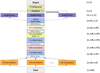 |
Fig. A.2 Overall structure of GaiaNet. Changes of tensor sizes are noted on the right side of the diagram. |
Appendix B Key spectral features compared to LAMOST
As shown in Fig. B.1, comparison of LAMOST/Gaia spectra of G-, K-, and M-type stars in CSTAR_XPM_nonG and a carbon star in CSTAR_XPM_G, focusing on the differences in spectral shapes observed under the resolutions of the two telescopes. We also reduced the resolution of their LAMOST spectra to observe changes in spectral shape. In Fig. B.2, we focus on comparing the feature correspondences between the LAMOST and Gaia spectra of a carbon star source, mainly observing the shapes of the absorption line regions of the LAMOST spectra and the band troughs of the Gaia spectra.
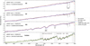 |
Fig. B.1 Spectra with the wavelength range intercept to 4400–9000 Å. The LAMOST spectra of some common sources are plotted with black lines. The red and yellow lines are the result of their convolution to 50 resolution. The blue and green lines are the Gaia spectra. In the bottom panel, the light gray shaded areas pick out the peaks and the red dashed lines in the bottom panels mark several obvious CN absorption line locations. |
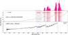 |
Fig. B.2 Example comparison of Gaia/LAMOST where the model explains the distribution of the most critical features (light gray areas) in the Gaia spectrum. The red gradient against a light gray background and the deep pink energy bar at the upper panel indicate the intensity of the feature SHAP values. The corresponding CN molecular absorption line positions (light blue dotted lines) are plotted in the LAMOST spectrum. |
Appendix C SHAP value statistics for carbon star candidates
The average SHAP value distribution of the features is shown in Fig. C.1. As can be seen from this figure, the sum of the average SHAP values (0.76164) of the 451 carbon star candidates is slightly lower than that of the positive sample (0.99894; see Fig. 4.2) but much larger than that of the negative sample (0.00056), which also confirms the reliability of our candidates. We also observed that the contribution of Feature 5 of the candidates almost disappears and that Feature 2 becomes weaker compared to the positive sample, which is consistent with the relatively weaker carbon signatures of their spectra.
C.1 Special negative feature
As shown in Fig. C.1, the negative feature near 8500 Å (Ca II absorption lines) becomes stronger than that in positive sample, this seems to imply that the candidates have greater metallicity (see Fig. 8 and Mallik 1997). It makes sense that our model treats this as a negative contribution to carbon star identification since metallicity tends to be positively correlated with the oxygen levels of a star’s atmosphere (Sanders & Matsunaga 2023). Another possible reason is that the neighboring molecular bands become weaker due to temperature or C/O ratio effect, thereby highlighting the Ca II absorption line features. Although there is a slight difference in the statistical distribution of SHAP values between the new candidates and positive sample, the overall characteristics suggest that the model is more inclined to classify them as carbon stars, indicating that these candidates are more similar to the golden sample carbon stars.
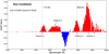 |
Fig. C.1 Same wavelength ranges from 6500 to 10000 Å. The average SHAP values across feature distributions are shown for the 451 new carbon candidates. |
Appendix D Heatmaps of six different stars
There are six sources in the results of Sanders & Matsunaga (2023) but are not in ours. Below, we explain the reason. We can see that Gaia 963568667249950592 (the first subplot of Fig. D.1) is an obvious problematic spectrum, our model also assigns it a small confidence level. The spectra in subplots 2-6 of Fig. D.1 have relatively weak absorption features in the region around 8000 Å and 9300 Å (i.e., Feature 1 and 2 in Table 4). Among these objects, Gaia 3586939158411536768 and 4056303080211083392 lack distinct CN molecular absorption band, then our model gives them lower confidence. Gaia 4314316918298388992 is weak in all Features 1-5, so the confidence level is also low. Gaia 4339500235641264256 has a stronger Feature 2, but a weaker Feature 1, resulting in a confidence level not exceeding 0.5. The molecular absorption bands of Gaia 5546572717982752640 are not prominent enough, so the confidence level is low.
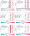 |
Fig. D.1 Interpretative heatmap of six C-rich star candidates for Sanders & Matsunaga (2023) that are not in our results. From top to bottom, left to right are sub-figures 1-6. The green dashed lines mark the positions used to calculate the CN band head strengths. 7732.9 Å and 8950.0 Å are the top of the band head, others are used to identify the location of band troughs. |
References
- Abia, C., Domínguez, I., Gallino, R., et al. 2002, ApJ, 579, 817 [NASA ADS] [CrossRef] [Google Scholar]
- Abia, C., de Laverny, P., Cristallo, S., Kordopatis, G., & Straniero, O. 2020, A&A, 633, A135 [NASA ADS] [CrossRef] [EDP Sciences] [Google Scholar]
- Abia, C., de Laverny, P., Romero-Gómez, M., & Figueras, F. 2022, A&A, 664, A45 [NASA ADS] [CrossRef] [EDP Sciences] [Google Scholar]
- Alksnis, A., Balklavs, A., Dzervitis, U., et al. 2001, Baltic Astron., 10, 1 [Google Scholar]
- Breiman, L. 2001, Mach. Learn., 45, 5 [Google Scholar]
- Carrasco, J. M., Weiler, M., Jordi, C., et al. 2021, A&A, 652, A86 [NASA ADS] [CrossRef] [EDP Sciences] [Google Scholar]
- Chen, Y. 2015, Master’s thesis, University of Waterloo, Canada [Google Scholar]
- Chen, T., & Guestrin, C. 2016, Association for Computing Machinery, 785 [Google Scholar]
- Cortes, C., & Vapnik, V. 1995, Mach. Learn., 20, 273 [Google Scholar]
- Cover, T., & Hart, P. 1967, IEEE Trans. Inform. Theory, 13, 21 [CrossRef] [Google Scholar]
- Efron, B. 1979, Ann. Statist., 7, 1 [Google Scholar]
- Gaia Collaboration (Creevey, O. L., et al.) 2023, A&A, 674, A39 [CrossRef] [EDP Sciences] [Google Scholar]
- Green, G. M., Schlafly, E., Zucker, C., Speagle, J. S., & Finkbeiner, D. 2019, ApJ, 887, 93 [NASA ADS] [CrossRef] [Google Scholar]
- He, X.-J., Luo, A. L., & Chen, Y.-Q. 2022, MNRAS, 512, 1710 [NASA ADS] [CrossRef] [Google Scholar]
- Herwig, F. 2005, ARA&A, 43, 435 [NASA ADS] [CrossRef] [Google Scholar]
- Hinton, G. E., Srivastava, N., Krizhevsky, A., Sutskever, I., & Salakhutdinov, R. R. 2012, arXiv preprint [arXiv:1207.0580] [Google Scholar]
- Ioffe, S., & Szegedy, C. 2015, in International Conference on Machine Learning, PMLR, 448 [Google Scholar]
- Ji, W., Cui, W., Liu, C., et al. 2016, ApJS, 226, 1 [NASA ADS] [CrossRef] [Google Scholar]
- Kim, Y. 2014, in Proceedings of the 2014 Conference on Empirical Methods in Natural Language Processing (EMNLP) (Doha, Qatar: Association for Computational Linguistics), 1746 [CrossRef] [Google Scholar]
- Kontizas, E., Dapergolas, A., Morgan, D. H., & Kontizas, M. 2001, A&A, 369, 932 [NASA ADS] [CrossRef] [EDP Sciences] [Google Scholar]
- Krogh, A., & Hertz, J. 1991, Adv. Neural Inform. Process. Syst., 4 [Google Scholar]
- Lebzelter, T., Mowlavi, N., Lecoeur-Taibi, I., et al. 2023, A&A, 674, A15 [NASA ADS] [CrossRef] [EDP Sciences] [Google Scholar]
- LeCun, Y., Bottou, L., Bengio, Y., & Haffner, P. 1998, Proc. IEEE, 86, 2278 [Google Scholar]
- Lépine, S., Rich, R. M., & Shara, M. M. 2003, AJ, 125, 1598 [CrossRef] [Google Scholar]
- Li, Y.-B., Luo, A. L., Du, C.-D., et al. 2018, ApJS, 234, 31 [NASA ADS] [CrossRef] [Google Scholar]
- Li, J., Long, L., Zhong, J., et al. 2023, ApJS, 266, 4 [Google Scholar]
- Li, L., Zhang, K., Cui, W., et al. 2024, ApJS, 271, 12 [Google Scholar]
- Lin, M., Chen, Q., & Yan, S. 2013, arXiv preprint [arXiv:1312.4400] [Google Scholar]
- Lippmann, R. 1987, IEEE ASSP Mag., 4, 4 [Google Scholar]
- Lundberg, S. M. & Lee, S.-I. 2017, in Advances in Neural Information Processing Systems, 30, eds. I. Guyon, U. V. Luxburg, S. Bengio, et al. (Curran Associates, Inc.), 4765 [Google Scholar]
- Mallik, S. V. 1997, A&AS, 124, 359 [NASA ADS] [CrossRef] [EDP Sciences] [Google Scholar]
- Morgan, D. H., & Hatzidimitriou, D. 1995, A&AS, 113, 539 [NASA ADS] [Google Scholar]
- Palmer, L. G., & Wing, R. F. 1982, AJ, 87, 1739 [Google Scholar]
- Polyak, B. T. 1964, USSR Computat. Math. Math. Phys., 4, 1 [Google Scholar]
- Qin, L., Luo, A. L., Hou, W., et al. 2019, ApJS, 242, 13 [NASA ADS] [CrossRef] [Google Scholar]
- Sanders, J. L., & Matsunaga, N. 2023, MNRAS, 521, 2745 [NASA ADS] [CrossRef] [Google Scholar]
- Secchi, A. 1869, Astron. Nachr., 73, 129 [Google Scholar]
- Shang, L.-H., Luo, A. L., Wang, L., et al. 2022, ApJS, 259, 63 [NASA ADS] [CrossRef] [Google Scholar]
- Si, J., Luo, A., Li, Y., et al. 2014, Sci. China Phys. Mech. Astron., 57, 176 [Google Scholar]
- Si, J.-M., Li, Y.-B., Luo, A. L., et al. 2015, Res. Astron. Astrophys., 15, 1671 [CrossRef] [Google Scholar]
- Sutskever, I., Martens, J., Dahl, G., & Hinton, G. 2013, in International Conference on Machine Learning, PMLR, 1139 [Google Scholar]
- Szegedy, C., Liu, W., Jia, Y., et al. 2015, in Proceedings of the IEEE conference on Computer Vision and Pattern Recognition, 1 [Google Scholar]
- Vassiliadis, E., & Wood, P. R. 1993, ApJ, 413, 641 [Google Scholar]
- Wallace, L. 1962, ApJS, 7, 165 [Google Scholar]
- Wei, P., Luo, A., Li, Y., et al. 2014, AJ, 147, 101 [Google Scholar]
- Werbos, P. J. 1988, Neural Netw., 1, 339 [Google Scholar]
- Zhang, B., Li, J., Yang, F., et al. 2021, ApJS, 256, 14 [NASA ADS] [CrossRef] [Google Scholar]
All Tables
Wavelength range and SHAP value score of the five most important features from the positive sample.
All Figures
|
Fig. 1 Main parameters of CSTAR_XPM sample. Panel a: Teff and log g diagram of CSTAR_XPM. Panel b: Spatial location and density distribution of CSTAR_XPM and random sample in the GBP − GRP and log g plane. The random sample (gray) is randomly selected from xp_sampled_mean. CSTAR_XPM stars are located in the giant star branch, with most having 2 < GBP − GRP < 5 mag; Panel c shows the distribution of golden sample carbon stars (red) and non-golden sample carbon stars (blue) in CSTAR_XPM. |
| In the text | |
|
Fig. 2 Images of normalized XP spectra of CSTAR_XPM_G. Upper panel shows a standard carbon star with four molecular band ranges marked in purple, and the red dotted line indicating the top of the band head. Middle panel shows three problematic spectra, while the bottom panel presents three spectra with very weak CN773.3 molecular band features. |
| In the text | |
|
Fig. 3 Six representative XP spectra from the 885 objects removed. The two prominent CN bands (purple areas) are located at the 7165–8108 Å and 8160–9367 Å ranges. The red dashed lines mark the top of the band head. The spectra are normalized and offset from one another by k × 1.0 + 0.2 for clarity (where k is an integer that varies from 0 to 6 from the bottom to the top spectrum). |
| In the text | |
|
Fig. 4 Alternative view from the C2023 sample of the 74 740 CSTAR_XPM_nonG (blue) flagged by ESP-ELS, 8176 selected positive training sample stars (red) from CSTAR_XPM_G, 8556 selected negative training sample stars (green) from CSTAR_XPM_nonG, and 885 deleted stars (yellow). The gray dashed line in the last subplot represents the boundary for the weakest CN strength. |
| In the text | |
|
Fig. 5 Venn diagram of the relationship of all samples in CSTAR (green frame). Spectra used are from CSTAR_XPM (purple frame, left in the figure). CSTAR_XPM_G is a cross between CSTAR_XPM and golden sample of carbon stars (purplish-red frame, right in the figure), and CSTAR_XPM_nonG is the complement of CSTAR_XPM and CSTAR_XPM_G. Negative sample (yellow) is selected from CSTAR_XPM_nonG, and positive sample (blue) is selected from CSTAR_XPM_G. Gray ellipse frame indicates range of possible carbon stars. |
| In the text | |
|
Fig. 6 Binary loss function depicted by contour line. The left panel shows the update path of standard SGD, while the right panel shows the path with momentum. The momentum-based update is smoother, more stable, and converges more easily to the global optimum. |
| In the text | |
|
Fig. 7 Distribution of CSTAR_XPM and the training sample on (MG)0 versus the (GBP − GRP)0 diagram. All the samples have been corrected for 3D extinction. Panel a: Distribution of the CSTAR sample. Panel b: Distribution of the training sample. Panel c: Distribution of carbon stars from the training sample. Panel d: Distribution of non-carbon stars from the training sample. |
| In the text | |
|
Fig. 8 Confusion matrix of our model predicted on the validation set. Label 0 represents a non-carbon star, and label 1 represents a carbon star. |
| In the text | |
|
Fig. 9 GaiaNet’s performance with the change of epoch numbers. Panel a: accuracy of the model on the training set (red) and validation set (blue); Panel b: number of misclassified spectra of the model on the validation set. |
| In the text | |
|
Fig. 10 Contribution ranking of features to the model result based on SHAP values. Each point represents a feature from the spectrum. The horizontal axis shows the SHAP values, while the vertical axis ranks the top 30 spectral features for identifying carbon stars, from most to least important. The color of each point indicates the size of the feature value. |
| In the text | |
|
Fig. 11 Feature heatmaps for individual spectral interpretations. The baseline is a background pseudo-continuum used to compute SHAP values, highlighting spectral features. The color indicates the SHAP value size: redder features contribute positively, while bluer ones contribute negatively to the model’s interpretation of carbon stars. The sum of SHAP values approximates the model output, with a larger sum indicating a stronger likelihood of the spectrum being identified as a carbon star. |
| In the text | |
|
Fig. 12 Average SHAP values per feature with a 20 Å wavelength bin size. Red and blue indicate positive and negative SHAP values, respectively. For comparison, the average spectra of positive and negative samples are overlaid as green scatter points. The upper panel highlights the two prominent CN bands with gray shading. |
| In the text | |
|
Fig. 13 XP spectra of eight candidate carbon stars similar to the normalization manner in Fig. 3. The yellow areas highlight key features we summarized. The blue dashed line marks the position of CN troughs, and the red indicates the peaks. |
| In the text | |
|
Fig. 14 Color-magnitude diagram (dereddened) of the new candidates (shown on the left) and the molecular band head strength of the new candidates (shown on the right). |
| In the text | |
|
Fig. 15 Spatial distributions of our results drawn in equatorial and Galactic coordinates. The gray spots denote the 15 400 golden sample of carbon stars. The blue spots represent the 8176 positive sample from CSTAR_XPM_G. The red spots are the 451 new carbon star candidates from CSTAR_XPM_nonG. |
| In the text | |
|
Fig. 16 Average distribution of SHAP values per feature for the G, K, and M types. The wavelength range is intercepted from 6500 to 10 000 Å. |
| In the text | |
|
Fig. 17 Relationship between band head strengths and confidence level, and with the sum of SHAP values. |
| In the text | |
|
Fig. A.1 Overall flowchart of GaiaNet. Convolution kernels of different sizes are used to extract features from different receptive field sizes. The arrows indicate the tensors of feature maps after convolution, pooling, or linear operations. A global max-pooling layer downsamples the feature map to compress its size and captures the most sensitive features. These are then combined into a tensor, which then undergoes GAP to share each feature value across the entire feature map. The resulting tensor is passed through a fully connected layer, which summarizes the features to produce a high-level abstract representation. Finally, a Sigmoid layer converts the neural network’s output into a probability distribution, making the predictions easier to interpret. Below the diagram, the corresponding convolution, pooling, and feature map shapes are labeled. |
| In the text | |
|
Fig. A.2 Overall structure of GaiaNet. Changes of tensor sizes are noted on the right side of the diagram. |
| In the text | |
|
Fig. B.1 Spectra with the wavelength range intercept to 4400–9000 Å. The LAMOST spectra of some common sources are plotted with black lines. The red and yellow lines are the result of their convolution to 50 resolution. The blue and green lines are the Gaia spectra. In the bottom panel, the light gray shaded areas pick out the peaks and the red dashed lines in the bottom panels mark several obvious CN absorption line locations. |
| In the text | |
|
Fig. B.2 Example comparison of Gaia/LAMOST where the model explains the distribution of the most critical features (light gray areas) in the Gaia spectrum. The red gradient against a light gray background and the deep pink energy bar at the upper panel indicate the intensity of the feature SHAP values. The corresponding CN molecular absorption line positions (light blue dotted lines) are plotted in the LAMOST spectrum. |
| In the text | |
|
Fig. C.1 Same wavelength ranges from 6500 to 10000 Å. The average SHAP values across feature distributions are shown for the 451 new carbon candidates. |
| In the text | |
|
Fig. D.1 Interpretative heatmap of six C-rich star candidates for Sanders & Matsunaga (2023) that are not in our results. From top to bottom, left to right are sub-figures 1-6. The green dashed lines mark the positions used to calculate the CN band head strengths. 7732.9 Å and 8950.0 Å are the top of the band head, others are used to identify the location of band troughs. |
| In the text | |
Current usage metrics show cumulative count of Article Views (full-text article views including HTML views, PDF and ePub downloads, according to the available data) and Abstracts Views on Vision4Press platform.
Data correspond to usage on the plateform after 2015. The current usage metrics is available 48-96 hours after online publication and is updated daily on week days.
Initial download of the metrics may take a while.