| Issue |
A&A
Volume 699, July 2025
|
|
|---|---|---|
| Article Number | A18 | |
| Number of page(s) | 19 | |
| Section | Interstellar and circumstellar matter | |
| DOI | https://doi.org/10.1051/0004-6361/202553893 | |
| Published online | 27 June 2025 | |
Understanding molecular ratios in the carbon- and oxygen-poor outer Milky Way with interpretable machine learning
1
Leiden Observatory, Leiden University,
PO Box 9513,
2300
RA Leiden,
The Netherlands
2
SURF,
Amsterdam,
The Netherlands
3
Transdisciplinary Research Area (TRA) ‘Matter’/Argelander-Institut für Astronomie, University of Bonn,
Bonn,
Germany
4
Department of Physics and Astronomy, University College London,
Gower Street,
London,
UK
5
INAF – Osservatorio Astrofisico di Arcetri,
Largo E. Fermi 5,
50125,
Florence,
Italy
6
Max-Planck-Institut für extraterrestrische Physik,
Giessenbachstraße 1,
85748
Garching bei München,
Germany
7
LUX, Observatoire de Paris, PSL Research University,
CNRS, Sorbonne Université,
92190
Meudon,
France
★ Corresponding author: This email address is being protected from spambots. You need JavaScript enabled to view it.
Received:
24
January
2025
Accepted:
8
May
2025
Abstract
Context. The outer Milky Way has a lower metallicity than our solar neighbourhood, but many molecules are still detected in the region. Molecular line ratios can serve as probes to understand the chemistry and physics in these regions better.
Aims. We used interpretable machine learning to study nine different molecular ratios to help us understand the forward connection between the physics of these environments and the carbon and oxygen chemistries.
Methods. Using a large grid of astrochemical models generated using UCLCHEM, we studied the properties of molecular clouds with a low initial oxygen and carbon abundance. We first tried to understand the line ratios using a classical analysis. We then proceeded to use interpretable machine learning, namely Shapley additive explanations (SHAP), to understand the higher-order dependences of the ratios over the entire parameter grid. Lastly, we used the uniform manifold approximation and projection technique (UMAP) as a reduction method to create intuitive groupings of models.
Results. We find that the parameter space is well covered by the line ratios, which allowed us to investigate all input parameters. The SHAP analysis showed that the temperature and density are the most important features, but the carbon and oxygen abundances are important in parts of the parameter space. Lastly, we find that we can group different types of ratios using UMAP.
Conclusions. We show that the chosen ratios are mostly sensitive to changes in the initial carbon abundance, together with the temperature and density. Especially the CN/HCN and HNC/HCN ratios are shown to be sensitive to the initial carbon abundance. This makes them excellent probes for this parameter. Only CS/SO is sensitive to the oxygen abundance.
Key words: astrochemistry / methods: numerical / methods: statistical / stars: formation / ISM: clouds
© The Authors 2025
 Open Access article, published by EDP Sciences, under the terms of the Creative Commons Attribution License (https://creativecommons.org/licenses/by/4.0), which permits unrestricted use, distribution, and reproduction in any medium, provided the original work is properly cited.
This article is published in open access under the Subscribe to Open model. This email address is being protected from spambots. You need JavaScript enabled to view it. to support open access publication.
1 Introduction
In the outskirts of our Milky Way lie giant molecular clouds (GMC), which play a crucial role in the process of star and planet formation. It is essential to understand the chemical composition within these clouds to understand the star formation process in the outer Galaxy (OG). In these parts of the Galaxy, the environment contains less oxygen and carbon than our own solar neighborhood (Esteban et al. 2017). This lower metallicity implies that there should be fewer atomic building blocks to build complex organic molecules (COMs). These COMs are molecules with more than six constituent atoms, and they are important for understanding the formation of prebiotic molecules (Herbst & van Dishoeck 2009). In recent observations, COMs were detected in several low metallicity environments, however, such as star-forming regions in the outer galaxy (Shimonishi et al. 2021; Bernal et al. 2021) and the Magellanic Clouds (Sewiło et al. 2018, 2022; Shimonishi et al. 2023), implying a chemical richness that is not expected in these environments. It is essential to study the chemical complexity as a function of metal-poor gas to understand the star and planet formation in these low metallicity regions better. Even more recently, the project Chemical complexity in the star-forming regions of the outer galaxy (CHEMOUT) observed 35 of these star-forming cores at the edge of our own Milky Way and confirmed their molecular richness (Fontani et al. 2022a,b; Colzi et al. 2022; Fontani et al. 2024).
The GMCs typically have a low temperature (T<100K) and number densities of nH > 100 cm−3. The astrochemistry within these clouds is driven by the fact that the gas is cold enough to freeze atoms and molecules onto the grains of the dust particles, which enables the ice chemistry. Within these ices, molecules can increase in complexity by reacting with one another (one of the main pathways is hydrogenation), and they then form larger molecules. With modern telescopes, these molecules can be detected at an unprecedented rate. This creates a compendium of many molecular observations with an increasingly complexity. Computational models are then used to simulate the astrochemical processes that produce and destroy molecules within these clouds. The great variety of possible physical conditions, chemical histories, and many different molecules mean that it becomes hard to interpret the observations, however. The uncertainties on the elemental abundances of a region further complicate the process. We attempt to circumvent this issue by investigating how several simulated molecular line ratios can be interpreted using machine learning.
In order to model the origin of the molecules in the outer regions of the Galaxy, we use the gas-grain chemical code UCLCHEM (Holdship et al. 2017) to model the regions as molecular clouds of constant density and temperature.
We then combine a classical analysis and interpretable machine learning to interpret a large grid of these models. The classical analysis of astrochemical models was extensively used to model and understand a variety of objects and astrophysical processes (Bayet et al. 2008, 2009; Wakelam et al. 2010; Bayet et al. 2011; Woods et al. 2012). They were only able to cover a relatively small part of the parameter space because neither the generation nor the interpretation of a large number of models was possible. With new machine-learning methods (Harada et al. 2024a) and especially interpretable machine-learning methods (Heyl et al. 2023b,a; Ramos et al. 2024; Grassi et al. 2025), the interpretation of large grids of models becomes feasible at once. Interpretable machine learning is a rapidly evolving field that is concerned with providing insight into how machine-learning models arrive at their prediction. The field of interpretable machine learning evolves rapidly because increasingly complex artificial-intelligence methods require investigations into why they work so well. However, interpretable machine learning can also be used as a tool to help us understand nonlinear and complex classical processes. We use the interpretable machine learning as a method to help us interpret our large parameter space. We specifically used the Shapley Additive exPlainers (SHAP) (Lundberg & Lee 2017). SHAP originated in game theory (Shapley & Shubik 1971) and is especially useful for understanding the nonlinear forward connections between input and output. These are here the physical parameters and ratios, respectively. The method quantifies the contribution of each of the input parameters to the output prediction by treating it as an additive game. In order to better understand our astrochemical models, we trained boosted regression forests and used the TreeSHAP algorithm to extract explainers for each of the ratios.
Since each model has six features and six corresponding SHAP contributions, the high dimensionality of the dataset remains. By plotting these together with a color map, we only have three dimensions that we can investigate at once. This severely limits the interpretability, however, because it requires a quadratic number of plots for an investigation of the effects of each feature independently, and the plots are often degenerate. To alleviate this problem, we introduced the Uniform Manifold Approximation and Project Technique (UMAP) (McInnes et al. 2020) constructed using the SHAP contributions and the ratio itself. This method resulted in a two-dimensional coordinate space, in which the models were arranged into a smooth manifold by grouping similar SHAP contribution vectors. By then using a color map to represent the ratio, features, and SHAP contributions, we investigated groups of ratios, their dependence on the physical parameters, and how SHAP clustered them. This allowed us to investigate the SHAP values in the most informative two-dimensional representation, and it separated the degeneracies present in classical two-dimensional plots.
In Section 2 we first describe the setup of the grid of astrochemical models and how we converted the models into mock observations of molecular line ratios. We then describe the theoretical framework of SHAP. In Section 3, we start with a classical analysis of the mock observations and then proceed to analyze the ratios using SHAP and UMAP. In Section 4, we conclude the paper.
2 Methods
Kinetic chemical codes have long been used to provide insight into the formation and destruction of molecules in various astronomical contexts, for instance, those discussed by Brown et al. (1988); Millar et al. (1991); Viti & Williams (1999); Ruaud et al. (2016); Rollig et al. (2007). These codes keep track of the total densities of various molecules as a function of time, space, and/or visual extinction, which provides insight into their formation and destruction mechanisms driven by physics and chemistry. We specifically modeled the objects in the outer galaxy as dark clouds, without any energetic source (e.g., hot core or shock models), which is consistent with the expected lower cosmic-ray ionization and radiation field in the outer galaxy.
2.1 Modeling dark clouds with UCLCHEM
The chemical composition in dark clouds was modeled using the open-source gas-grain chemistry code UCLCHEM (Holdship et al. 2017). This code allowed us to model the gas and grain chemistry in a time-dependent manner. This provided us with timeseries that describe the abundances of each of the molecules in the model. The modeling assumed istothermal clouds with a constant density. For these clouds, we then varied six parameters: the number density, temperature, the cosmic-ray ionization rate, the UV radiation field, the initial elemental abundance of carbon, and the initial elemental abundance of oxygen. We explored cold molecular cloud models with several densities that ranged from 103 cm−3 to 107 cm−3 and temperatures of up to 100 K. The cosmic-ray ionization rate reached from the typical galactic value (Indriolo et al. 2007) to 103, and the UV radiation field ranged from 0.1 to 10 Habing. The elemental abundances of carbon and oxygen were depleted independently by up to a factor of 20 compared to solar values (Fontani et al. 2024; Méndez-Delgado et al. 2022). The range of all values and whether we sampled them in a linear or logarithmic fashion can be found in Table 1. The initial elemental abundances for the atoms that were not varied in the grid can be found in Appendix A. The models were ran up to a time of 107 years each; with a cloud radius of R = 0.5 pc, which is consistent with the lower limit of the regions in Fontani et al. (2024). This resulted in clouds with visual extinctions of AV = 2.0 at the lowest densities. This included an edge visual extinction of 1 mag. At the highest density, the visual extinctions reached up to AV ∼104.
In order to alleviate the curse of dimensionality of our six-dimensional parameter space, we used Sobol sequence sampling (Sobol’ 1967). Uniform random sequences are often used to sample these spaces, but they have a high discrepancy. The high discrepancy can become a problem when the output of these nonlinear models is to be analyzed. Another method would be to use grid or Latin-hypercube sampling, which both guarantee that the marginal distribution for each of the parameters is uniform. Grid sampling quickly becomes intractable, however, and Latin-hypercube sampling does not guarantee a low discrepancy either. Sobol addresses the computational and discrepancy shortcomings and allowed us to efficiently investigate the parameter space. This resulted in a grid of 216 = 65536 models. Some of these models did not run successfully, however. This can be attributed to certain computationally stiff regimes where the freeze-out onto the grains and desorption compete, which causes the timescales of the reactions to become extremely short and expensive to solve. In this case, UCLCHEM chooses not to integrate until the final time. We experimented with treating these missing data by excluding the data points and substituting the final value for the last-known value. The former method was most effective because the latter tended to create spurious ratios that did not agree well with the distribution of neighboring parameter sets. We therefore excluded spurious data points. With all the abundances simulated as a function of time, we computed the molecular line ratios. We chose to compute the ratios at 105 years. At this time, the gas-phase species have not had a chance to fully freeze-out onto the grains. This allowed us to investigate a relatively young astrochemistry on the formation timescale of a young stellar object (Williams 1998). In order to account for the fact that molecules with a low number abundance cannot be observed, we took the abundances for the model and filtered them based on a minimal abundance that is needed to result in an observable intensity. We took the lower limit of xi ≥ 10−12 because this is conservatively the lowest abundance we can observe. Any ratios with a nondetection in either its enumerator or denominator were therefore not taken into consideration. This provided the dataset of molecular ratios, which can help us understand the forward relation between the physical conditions and the chemical composition.
Parameter grid.
2.2 Molecular ratios as tracers of physical conditions
To probe the physical conditions and the chemical composition of various astrophysical regions, molecular line ratios serve as an essential diagnostics. On an extragalactic scale, they were used extensively to characterize starburst galaxies (Harada et al. 2024a; Butterworth et al. 2022) and active galactic nuclei (König et al. 2018; Usero et al. 2004; García-Burillo et al. 2010). On a galactic scale, ratios were used to characterize molecular clouds (Peñaloza et al. 2018; Tafalla et al. 2021). We propose the use of three main groups of ratios, namely methanol-based, hydrogen cyanide-based, and finally, sulfur-based ratios, many of which have been used to probe different physical conditions and environments. The ratio of H2CO/CH3OH is connected to the formation of COMs in the ice phase and can also serve as a probe of the formation timescales of massive star formation (Sabatini et al. 2021). When combined with cyclopropenylidene, the C3H2/CH3OH ratio was employed to constrain the effects of the interstellar radiation field on starless cores (Spezzano et al. 2020) To further probe the formation processes of methanol, we also combined it with its first hydrogenated precursor, HCO, which provides insight into the formation pathways (Bacmann & Faure 2016). Physical conditions can also be probed by ratios such as HNC/HCN. This ratio is currently discussed as a possible strong predictor of the radiation field (Harada et al. 2024b), cosmic-ray ionization (Behrens et al. 2022), or temperature (Hacar et al. 2020). Another HCN-based ratio is HCO+/HCN, which can trace energetic environments such as AGNs (Butterworth et al. 2022). We also included the CN/HCN ratio because it is sensitive to the carbon and oxygen abundances (Milam et al. 2005), which serve as an effective tracer of dense gas (Wilson et al. 2023) and is associated with evolved starbursts (Harada et al. 2024a). The first sulfur-based ratio we investigated is CS/SO, which can directly probe the oxygen-to-carbon ratio in protoplanetary disks (Semenov et al. 2018; Gal et al. 2021) and provides a chemical clock for massive star formation (Li et al. 2015). The molecular ratio SiO/SO can be used to infer physical parameters of energetic systems (e.g., shocks) with grain processing (James et al. 2021; Codella & Bachiller 1999). Last, CS/CN can be used as a dense-gas tracer (Wang et al. 2022). We then proceeded with analyzing these ratios using interpretable machine learning.
2.3 Interpretable machine learning with SHAP
Modeling the chemistry of astronomical objects with grids of chemical model data is one of the classical methods for understanding the forward connection between physical and chemical parameters and molecular abundances and ratios. In the past, the application of computational models in astrochemistry was constrained by the computational cost of running them for different parameter configurations. Computational resources are great enough today that we can generate large volumes of simulations. This introduces the problem that high-dimensional simulation grids with several output ratios become increasingly hard to interpret by hand. Historically, conditional and marginal plots were the method of choice to interpret parameter studies, but they disregard higher-order interactions and require extensive expert knowledge for an interpretation. Interpretable machine learning addresses this by providing model-agnostic methods for understanding nonlinear models. Model-agnostic interpretation methods can be easily cast into a sampling, intervention, prediction, and aggregation framework (SIPA) (Scholbeck et al. 2019), and they are distinguished into two broad subcategories, global and local methods. Global methods are similar to the methods that astrochemists extensively used in the astrochemical literature, namely partial dependence plots, and more recently, even surrogates for principal component analysis. We therefore focused on the usage of local methods because they can provide more insight into subregions of the dataset by explaining the individual examples. This was shown to be a powerful tool in astronomy (Heyl et al. 2023b,a; Ramos et al. 2024; Grassi et al. 2025), but also in fields such as geophysics and biomedicine. Two current popular global method are local interpretable model-agnostic explanation (LIME) (Ribeiro et al. 2016) and SHAP (Lundberg & Lee 2017); the former tries to construct local surrogates for each individual prediction, whereas the latter tries to provide explanations by using a global interpretation method. We chose SHAP because we are interested in the behavior of the ratios throughout the entire physical range and its subsets and not in a sensitivity study of individual samples.
SHAP is an efficient approximation of the game-theory concept of Shapley values. These Shapley values are a method for evaluating how much a feature contributes to the output of a model by considering all possible player coalitions and the cost of each of them. An illustrative example is sharing a cab that brings several individuals home, where each addition or removal of a person to the coalition results in a different cost (Molnar 2022). This can be formalized into a Shapley value ϕ j for each feature j. These values satisfy the following properties:
Efficiency – all feature contributions together must sum to the output minus the expected value of the model.
Symmetry – when two features contribute equally across all coalitions, their SHAP value is identical.
Dummy – when a feature does not change the output, its Shapley value is zero.
Additivity – when two games are added together by summing the outputs, the SHAP values are the sum of the Shapley values of the individual game.
Unfortunately, the explicit computation of the Shapley values can quickly become prohibitively expensive as all coalitions must be evaluated for the exact value to be obtained. SHAP addresses this issue by instead computing the contribution of each feature as the weighted average of the marginal contributions. This shows us that each prediction must be a sum of the feature explanations plus the expected value of the predictor,
![Mathematical equation: \[\hat g(x) = \mathop \sum \limits_j {\phi _j} + (g(x)).\]](/articles/aa/full_html/2025/07/aa53893-25/aa53893-25-eq1.png) (1)
(1)
The Shapley value ϕj, also referred to as impact or contribution, determines how much each feature (e.g., density) has contributed to one realization (e.g., SiO/SO) according to the model. Concretely, we used the contributions to quantify the impact of each individual feature on each ratio sample.
This marginal contribution for each feature can be approximated in several ways, such as a linear explanation model with kernelSHAP (Lundberg & Lee 2017), a neural network with deepSHAP (Chen et al. 2019), and a forest model treeSHAP (Lundberg et al. 2020). We used the latter because it provides a computationally effective method that is particularly well suited for the pregenerated tabular data on a grid, but instances of deepSHAP have also been used in astronomy (Ramos et al. 2024; Grassi et al. 2025). As the name suggests, treeSHAP relies on decision trees. For this specific use case, we used boosted regression forests. Regression forests are a combination of decision trees that use continuous data, and boosting refers to the concept of sequentially combining weak predicting trees that become a strong predictor when they are combined into an ensemble (Hastie et al. 2009). The structure of the tree, descending down a path of decisions, constrains the number of possible coalitions. This alleviates the computational complexity of computing the SHAP values.
2.4 Uniform manifold approximation and project technique
In order to reduce datasets to lower dimensions, the uniform manifold approximation and projection technique was developed (McInnes et al. 2020). Similar in nature to PCA (Pearson 1901) and t-SNE (van der Maaten & Hinton 2008), it allows one to create a lower-dimensional representation of high-dimensional data that can aid in clustering, interpretation, and feature importance. The method assumes that the data points lie on a Riemannian manifold within a high-dimensional space and tries to find a mapping between the two that preserves the local and the global structure. These resulting low-dimensional manifolds have been shown to help greatly in the classification in several astronomical contexts such as auroral dynamics (Lamb et al. 2019), fast radio bursts (Chen et al. 2022), and low-metallicity stars (Kane et al. 2023).
The algorithm tries to construct a weighted graph in high-dimensional space by connecting neighbors. By constructing the K nearest-neighbor (KNN) graph, it captures the local structure of the data. It can then construct a mapping function between the high-dimensional space onto the lower-dimensional space, trying to preserve the nearest neighbors with a cross-entropy loss function.
Because our dataset was sampled on a regular grid and we only have the ratio as a meaningful feature, the KNN algorithm does not perform well when it tries to construct a meaningful representation. When we interpret the impact of each feature as a component of a vector, however, one SHAP explanation can be seen as a six-dimensional vector whose values add up to the ratio. We used these six SHAP features together with the ratio as the input into the UMAP algorithm. The most important hyper-parameters are the number of neighbors k, the minimum distance between points, the low-dimensional representation dmin, and the weighting of the loss of the SHAP values versus the loss of the ratios themselves wratio. After manually tuning these, we chose k = 100, dmin = {0.1, 0.5} and a wratio = 0.1. The goal of this tuning was to obtain a smooth manifold that was not too compact but still clustered. This allowed the manifold to highlight different regions and changes as a function of the parameters. The chosen set of parameters reflects a good trade-off between these two extremes. The loss for the SHAP features was computed using the cosine distance, and the loss for the ratio was computed using Euclidean distance. This reflects the fact that we treated the SHAP contributions as a vector, whereas the ratio was added as measure to break degeneracies in the aforementioned vector space.
2.5 Interpreting molecular line ratios with SHAP
As described in Section 2.1, we started by using UCLCHEM to simulate each of the models on the parameter grid. This then resulted in a time series for each molecule. From this time series, we obtained the value at 105 years. We then applied the observational threshold for each molecule, when either the denominator or the enumerator exceed the observational threshold, we computed its log-value and added it to the dataset.
With a dataset for each ratio, we split it into a training set and a test set that contained 70% and 30% of the set respectively. The training dataset was used to train a regression forest, with the physical parameters as input and the molecular line ratio as output. The hyperparameters of the regression forest were optimized using the Optuna framework (Akiba et al. 2019) with the test error as the optimization target. We took the optimal configuration and trained the regression forest again to generate the final predictor model. The SHAP values were then computed using this regression forest and the TreeSHAP algorithm as implemented in the SHAP package (Lundberg & Lee 2017). This resulted in the SHAP values for each sample in the dataset. This was then repeated for each molecular line ratio, resulting in nine distinct regression forests and SHAP explainers. Finally, we fed these SHAP values and the ratios into the UMAP algorithm. This resulted in a two-dimensional embedding for the data and helped us to interpret the SHAP values, input features, and ratios.
3 Results
In order to better understand the SHAP contributions, we first analyzed the results in line with a classical sensitivity study of the ratios and their dependence on temperature and density. We then studied the relative importance of each input feature by investigating the order of importance and the nonlinearity of its impact. Last, we investigated the impact further by plotting the ratios, feature values, and impacts on a low-dimensional manifold, for which we grouped similar models together and revealed the nonlinearities in the ratios.
3.1 The molecular ratios: From chemical modeling to observable abundances
Before we reduced the fractional abundances to a ratio, we first inspected the distribution of the two species with respect to each other. A plot of the two constituents of each ratio is displayed in Figure 1. We distinguished between four scenarios: only A is detected, both A and B are detected, only B is detected, and last, neither are detected. This is represented by the four regions in the figures, and the dashed lines represent the observational limits. For every one of the ratios, part of the distribution lies in the range in which both molecules can be detected.
In order to extract as much information out of the grid of models as possible, we chose to include any sample that detected either molecule. Even though the more extreme ratios in the region in which only one molecule is detected cannot be observed directly, they can still be useful when they are combined when an upper limit can be derived from the observation. The distribution of all ratios can be found in Figure 2. The statistics for the ratios filtered by either detection can be found in Table 2. In the rest of the analysis, the data were always filtered for a detection in either molecule.
In order to visualize the dependence of the ratios on the temperature and density, we plot the ratios as a color map, as shown in Figure 3. A plot with the denominator and enumerator of the fractional abundance of the ratioscan be found in Appendix D.
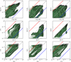 |
Fig. 1 Fractional abundances for each of the ratios. The contour levels of a kernel density estimate are added to highlight the distribution, each representing 20% of the distribution. For both, we show the observational limit of 10−12 that we used throughout. Only the ratios above either observational threshold were used to train the SHAP explainers. The blue line represents all log-ratios of −12, and the red line represents the log-ratios of 12. |
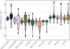 |
Fig. 2 Distribution of each of the ratios that exceeded the detection limit for both molecules. The left distribution for each ratio shows where both molecules are detectable, and the right distribution shows this for each molecule where either molecule is detectable. The line in the central box is the median, the central box contains 50% of the ratios, the next upper and lower boxes together contain 25% and so forth, and the outliers plotted as diamonds. |
3.1.1 Methanol-based ratios
Starting with the upper left ratio, H2CO/CH3OH, there are two general distributions in density-temperature space: a lowdensity distribution with densities up to 106 cm−3, and a high-temperature density distribution with densities higher than 106.2 cm−3 and temperatures starting at 87 K.
The low-density distribution is split into two parts, with a division at 30 K. Below this division, the formation of methanol and formaldehyde occurs quickly and at a positive ratio, and at t = 105 years, both species peak in the gas phase and then quickly completely freeze out onto the grains. Above this division, the formation pathway of methanol on the grain becomes much less efficient, and less methanol can be desorbed into the gas phase, but the formation of formaldehyde is not affected as much. This results in a positive ratio because methanol is barely above the detection threshold, but formaldehyde achieves fractional abundances of up to 10−8.
The general pattern of the C3H2/CH3OH ratio is similar, but it lacks the distribution with a very negative log-ratio below 30 K and a clear gap between the low and high densities. The negative distribution below the threshold in the low-density regime is due to the less effective formation of C3H2 at these lower temperatures, while methanol still peaks. This distribution is intersected by the blue line in Figure 1. Above this border, the formation of C3H2 increases, resulting in positive ratios. For the high-density temperature distribution, C3H2 already decreases, while the CH3OH peaks, resulting in a negative ratio.
The last methanol-based ratio, HCO/CH3OH, has a negative high-temperature density distribution. Again, in the main distribution, a division at 30 K is present, with a negative horizontal gradient between temperatures of 30 and 45 K. Between these temperatures, as the density increases, the methanol becomes more abundant, with HCO being relatively constant in abundance. At densities well above nH = 105 cm−3, HCO starts to freeze out, while methanol is still more abundant, resulting in a small region with negative ratios at low temperatures. Below 30 K, the methanol becomes very abundant in the gas phase. This results in an even more negative ratio for this region. Above 45 K, the formation of methanol is again less efficient, while HCO is more abundant and depletes at a slower rate, resulting in positive ratios. The high-density temperature distribution has only detections of methanol, resulting in very negative distributions. This is also reflected by the distribution that intersects the blue line in Figure 1.
3.1.2 HCN-based ratios
The hydrogen cyanide ratios are detectable almost everywhere, with the exception of the high-density low-temperature part of the parameter space.
The leftmost part of the distribution is dominated by the photodissociation of HCN into CN, resulting in a positive ratio. As the density increases, the ratio starts to tend toward being dominated by HCN. In the lower right area, at temperatures below 40 K and densities above nH = 105 cm−3, the chemistry is dominated by a fast freeze-out of CN, while HCN freezes out on a slower timescale. For the HCO+/HCN ratio, a similar pattern emerges, but now without positive ratios in the right part of the distribution. At lower densities, the ratio is close to unity, but as the density increases, there is less photochemistry and the log-ratio becomes increasingly negative. The isomer ratio HNC/HCNonly has negative log-ratios, driven by an effective isomerization pathway at higher temperatures: H + HNC → HCN + H (Hacar et al. 2020). The log ratio is closest to being zero in the high-temperature and very low-temperature regime, with densities between 104 and 106.5 cm−3. In the other regions, HCN strongly dominates HNC.
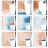 |
Fig. 3 Distribution of the log of the ratios as a function of the density and temperature. |
3.1.3 Sulfur-based ratios
The sulfur-based ratios trace out a similar region of the parameter space. The CS/SO log-ratio is positive in most of the parameter space, and only at the lowest temperatures of the densities above nH > 105 cm−3 does the ratio become negative. This local negative ratio occurs as CS starts to freeze out, while SO does not. The SiO/SO ratio and the CS/CN show a similar pattern in the parameter space. However, for the latter, an interesting split is visible along the diagonal of the upper right of the parameter space. Below the split, the log-ratio is zero because CS and CN reach high abundances. Above the split, the CN is depleted, causing the log-ratio to become positive.
This exploration of the distribution of the ratios in temperature-density space provides the context for the explainable machine-learning methods. We investigated the order of importance of the physical parameters to better understand what influences the ratios most.
3.2 Mean SHAP impact. Ranking the physical features
For each of the models, we computed the normalized feature importance, which is defined as the individual contribution divided by the sum of the contributions for each ratio. This explains the relative importance of each feature per ratio. We plot its values for each ratio in the heat map in Figure 4. The importance confirms that the temperature and density are almost always the most important features, and the oxygen and carbon abundances are sometimes close contenders. For example, for CS/SO, the carbon abundance is more important than the number density, which agrees with the temperature-density distribution in Fig. 3, where the gradients of the ratios are small in the direction of the density. This order of features is useful for distinguishing how sensitive features are, but it does not capture any information about how the ratio is impacted exactly as a function of each feature. Here, SHAP summary plots add information.
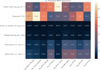 |
Fig. 4 Relative importance of each physical parameter for all of the ratios. |
3.3 SHAP summary plots. Interpreting first-order interactions
The SHAP summary plots as shown in Figure 5 show a scatter point for each feature for each of the samples. Each sample is then represented by six points across the parallel feature axes, with each impact color-coded with its respective value. A positive SHAP contribution means that the log ratio was increased by the feature value, and vice versa.
For all the methanol-based ratios, the most important feature is the temperature. The contribution of the temperature ϕT increases monotonously with its value for all ratios. The impact of the density  is second, and is inversely proportional to the density. The impact of carbon and oxygen are the third (inversely proportional to the feature value) and fourth (proportional to the feature value) most important features, respectively.
For the HCN based ratios, the density is the dominant feature, and its impact is inversely proportional to the density. For the first and third HCN- based ratios, CN/HCN and HNC/HCN, carbon is the second most important feature, and temperature is third. For HCO+/HCN, the temperature is the second most important feature, and its shows no monotonous increase or decrease in impact. Interestingly, for HNC/HCN, the temperature is not the most important feature, which contradicts what has been found before, at least at low temperatures (Hacar et al. 2020), as well as the feature importance findings by Heyl et al. (2023a), where temperature had the strongest impact. These models used two modeling stages, in combination with higher densities and temperatures, whereas our models assumed static clouds. The total metallicity by Heyl et al. (2023a) and the initial carbon abundance in this study are both the second most important features, which is consistent between the two SHAP explainers. CS/SO is a ratio that strongly depends on temperature, and the carbon abundance closely follows. For the SiO/SO ratio, the density is now the second most important feature, but the distribution of its impact is complex. The last ratio, CS/CN, shows a strong impact for density, and the minimum and maximum densities contribute negatively, while medium densities have a positive impact. The carbon dependence shows a clear proportional relation. The temperature is inversely dependent, with a medium temperature distribution with negative impact. Last, the oxygen dependence shows a clear inverse proportional dependence.
The individual impact of each feature, while providing insight into the ratios, does not tell us how two features depend on each other. In order to reveal higher-order dependencies, we therefore relied on dependence plots, which show the dependence of one impact on the feature itself and on others.
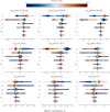 |
Fig. 5 All of the SHAP values for each of the ratios. The features are sorted by mean absolute impact as shown in Figure 4. Every color map is normalized to the detectable range for each individual feature per ratio. |
3.4 UMAP plots. Interpreting higher-order interactions
The main benefit of using a statistical predictor and computing its SHAP values is that we can now interpret the dependences between the different features and the ratios themselves. The UMAP manifold was generated using the SHAP impacts and the ratios themselves, creating a convenient two-dimensional representation of the data, where local and global features are relevant. This allowed us to identify distinct groups of models that behaved similarly, and to determine how the features influence the ratio within these groups.
We analyzed the ratios projected onto a two-dimensional manifold computed using the SHAP values and ratios. In this way, we investigated the clustering of similar models and determined their dependence on the input features.
3.4.1 H2CO/CH3OH
For the H2CO/CH3OHratio, the UMAP plot is shown in Figure 6. This plot shows that we can cluster the high-temperature and low-density models on the top left side of the manifold, with a positive impact of both features. This results in very positive ratios.
At the bottom of the manifold, the temperature is low and the density is low as well. In this case, the contribution of the temperature is negative, and the contribution of the density ranges from small to negative. The two lobes in the right part of the plot are especially interesting. These regions correspond to the hidden distribution, as shown in top right corner of Figure 3. For the middle distribution, the impact of the temperature is clearly positive, with a slightly negative density impact, a low carbon abundance, but a very positive carbon impact, a high oxygen abundance, and also a positive oxygen impact. The rightmost lobe, on the other hand, has a high carbon abundance distribution, with neutral temperature impacts, very negative density impacts, high carbon abundances with negative impact, and last, a gradient in the oxygen abundance, with an impact that extends from very negative to positive. This is all related to the distribution of methanol-dominated ratios.
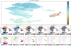 |
Fig. 6 H2CO/CH3OH ratio, feature, and SHAP values plotted on a two-dimensional manifold using the ratio and the SHAP values. The manifold consists of a broad left region with two separate right lobes. |
3.4.2 C3H2/CH3OH
We investigated the UMAP manifold, displayed in Figure C.1, which clusters the distribution into three regions. The left region contains the lowest-temperature gas, which has a negative temperature contribution. As the density increases along the vertical axis, the SHAP contribution for the temperature decreases. In this region, the carbon impact is negative, without a clear pattern in its value. The oxygen value, however, shows a clear radial gradient that is connected with a negative SHAP contribution in the center of the region and a positive one on the outskirts.
The right and more extended region contains the medium-temperature low-density gas, with positive contributions. The carbon abundance shows a clear gradient from positive to negative with increasing depth, and the SHAP contribution evolves from positive to negative. The pattern for oxygen is radial, and the inner region has negative contributions with low values, and the outer region has positive contributions. Last, there is a lobe at the bottom: this is the high-temperature high-density gas, with a positive temperature impact and a negative density impact. The contributions of carbon and oxygen clearly influence the ratio.
3.4.3 HCO/CH3OH
The manifold for this ratio is displayed in Figure C.2. It shows an elongated distribution of the gas. The continuous part of the manifold contains the distribution of warm gas on the right side, with low to medium densities. This gas has positive temperature contributions with negative to positive density contributions. The oxygen and carbon abundances increase in value farther outside of the manifold. The distribution on the left side, on the other hand, consists of the cold gas with low to medium densities. The ratio is mostly impacted by the negative-temperature contribution, combined with a positive to negative density contribution. Similarly, the carbon and oxygen values are distributed in the radial direction. Last, there is also a separated distribution in the bottom left corner; this again consists of the high-temperature high-density gas. It is again influenced by the carbon and oxygen content, and the ratio increases from the bottom left to the top right corner from low to high oxygen and carbon.
3.4.4 CN/HCN
The manifold is displayed in Figure C.3. It is separated into four distinct regions, the bottom left, left, right, and top part. The bottom left region is strongly dominated by HCN. It mostly contains low-temperature models, high carbon abundances, and intermediate densities. The adjacent left distribution is dominated by higher-density gas, but now shows a clear split with respect to the carbon abundance. Left of this split, the carbon abundance is higher, while on the right, the carbon abundance is lower. This split continues into the right distribution of positive ratios with lower densities, with the top having a low carbon abundance and the bottom higher values. Last, there is a distribution of top right models with medium densities and very low carbon abundances. These models have a positive ratio, which is mostly explained by the positive impact of low-carbon, high-oxygen, and medium-temperature models.
3.4.5 HCO+/HCN
The manifold for this ratio is shown in Figure C.4. Across the horizontal axis, the density increases from left to right, while the ratios decrease. In the bottom left corner, there is a low-density low-temperature region with ratios similar to those in the top right distribution, but now explained by a positive density impact and negative temperature impact. The top left low-density region consists of HCO+-dominated gas, while the gas in the top right corner is dominated by HCN. The bottom right corner then contains a region with high-temperature gas and high densities, but neutral ratios as the impacts sum to zero.
3.4.6 HNC/HCN
We investigate the manifold for this ratio in Figure C.5. It shows no clear separation between the regions, but more of a continuous shift, with only a HCN-dominated area at the bottom. This agrees with the isomer chemistries, which are similar in nature. The large region spanning the rightmost part of the plot is dominated by models with a small positive SHAP impact, resulting in a neutral ratio. At the bottom lies a region in which HCN starts to dominate strongly. These models are low in carbon, with an associated negative carbon impact and a negative oxygen impact. This indicates that in order to obtain strongly HNC depleted models, we need low carbon abundances. Last, the upper left part of the distribution shows that the ratio is again closer to being neutral.
3.4.7 CS/SO
The manifold, as shown in Figure C.6, shows a complex but continuous pattern, where the temperature impact varies strongly across the vertical axis, while the horizontal axis varies the carbon impact. There is a distinct region in the center where the density impact is very positive, and its values are low. In the top to middle distribution, the ratios indicate a SO-deprived chemistry, with low carbon abundances. In the bottom right part of the distribution lie models with negative values, mostly driven by gas with medium temperatures and high densities.
3.4.8 SiO/SO
The UMAP manifold is displayed in Figure C.7. This shows a distribution split between top and bottom regions with mostly high and low temperatures, respectively. The left part of the manifold corresponds to regions that are dominated by SIO. In the rightmost high-density region lies a distribution that reaches negative values as the SO is enhanced around 50 K.
3.4.9 CS/CN
The manifold, as shown in Figure C.8, contains two large distributions, and a smaller distribution at the bottom. The right distribution consists of gas with a negative-density contribution, creating values that are close to zero, and even more negative at the edges, where the radiation field has a negative impact. This shows that at low densities and high radiation fields, the impact of the radiation field becomes important. This can be attributed to the fact that CN is related to photochemistry, as shown in the CN/HCN ratio before. Moreover, the contribution to the radiation field strongly depends on the density. As it increases at low densities, it correctly lowers the ratio. The regions at the top are also dominated by CN, but these models are instead related to a very negative carbon abundance impact. With high densities and low carbon abundances, the ratio becomes negative.
The distribution at the bottom, on the other hand, contains high-carbon models, with low temperatures and medium densities. This results in a depletion of the CN chemistry. The region in the lower left corner contains a broader distribution of models with a generally positive density impact, high densities, and high temperatures, resulting in a similar but less extreme scenario.
4 Discussion and conclusions
Our results indicate in general the physical parameters that are most important for chemistry and that can therefore be constrained with molecular observations. Temperature and density are generally the most important features. Therefore, observers that would like to use molecular observations to constrain other physical parameters first need to probe temperature and density accurately. However, our study also suggests that not all the inspected physical parameters are relevant in the investigated molecular ratios. For example, at these low temperatures and at this reduced metallicity, they cannot constrain the cosmic-ray ionization rate, which hence would need to be estimated based on other molecular species or with other methods. This result was also found by Fontani et al. (2024), who used the technique we presented here: The investigated molecular ratios indeed cannot constrain the cosmic-ray ionization rate in the interval of the values we studied (∼10−14–10−17 s−1). Some ratios are more sensitive to metallicity than others, and in particular, more sensitive to carbon abundance variations, as we describe below. Therefore, these ratios could also be used to test the metallicity gradients derived from observations. For example, the carbon and oxygen elemental abundances decrease with the galactocentric distance according to observations up to ∼14– 16 kpc (e.g., Arellano-Córdova et al. 2020; Méndez-Delgado et al. 2022). These gradients are usually extrapolated to larger distances, where we lack observations. Our method allowed us to verify whether this extrapolation is correct. By measuring molecular ratios at galactocentric distances larger than 16 kpc, as was done, for example, in the CHEMOUT project, we can test whether the measured molecular ratios are consistent with models in which the elemental abundances decrease, as predicted by the extrapolated gradients.
We used a comprehensive grid of astrochemical models to understand the forward connection between the physical modeling parameters and the observable line ratios. The nine ratios we chose to inspect cover a large part of the physical parameter space, with the exception of low-temperature high-density regimes. We specifically focused on the influence of lowering the initial elemental abundances of carbon and oxygen. We used SHAP as a method to explain the impact of each feature on the modeled ratio. This showed that especially the impact of the carbon and oxygen initial elemental abundances can be on par with temperature and density. We also showed that these SHAP explanations can be paired with UMAP to provide insightful lower-dimensional groupings for the models. We conclude the following about the molecular line ratios in this study:
The temperature and density are generally the most important features, but the cosmic-ray ionization is negligible. This may be partially explained by the fact that the gas-grain model we used does not compute the temperature balance (and hence, the temperature is independent of the cosmic rays). This isolates their effect to the cosmic-ray chemistry alone.
Ratios such as CN/HCN and HNC/HCN can be sensitive to the initial carbon abundance, which makes them important for constraining the metallicity.
There is a distinct range of very negative CN/HCN and HNC/HCN models with a low carbon and high oxygen signature.
The methanol-based ratios strongly depend on temperature and density, but in regions with a high temperature and high density, carbon and even oxygen abundances can have a strong impact.
The HCO– and HCO+-based ratios depend little on the oxygen and carbon abundance in this parameter space.
The sulfur-based ratios strongly depend on the carbon ratio, with distinctly different regions of temperature and density. This allowed us to effectively constrain the carbon ratio with observations.
None of the chosen ratios are particularly sensitive to the initial oxygen abundances, and CS/CN depends most on oxygen.
These analyses can be used in order to inform new forward model studies, but also the backward interpretation of observations, by better informing the priors of a Bayesian analysis.
Acknowledgements
We thank the anonymous reviewer for their insightful comments and suggestions, which helped improve this manuscript. G.V., F.F. and S.V. acknowledge support from the European Research Council (ERC) Advanced grant MOPPEX 833460.
Appendix A Elemental abundances
The initial elemental abundances used in UCLCHEM and the depletion of the initial carbon and oyxgen abundances are listed in Table A.1.
Initial elemental abundances used in UCLCHEM. The number density of hydrogen nuclei is 
Appendix B Hyperparameter optimization
The best hyperparameters for the xgboost regression forests (Chen & Guestrin 2016) after 500 trials using Optuna (Akiba et al. 2019) can be found in Table B.1
The ranges for each hyperparameter and the best configuration found after 500 trials with Optuna (Akiba et al. 2019).
Appendix C UMAP plots
This appendix contains all the remaining UMAP plots for C3H2, HCO/CH3OH, CN/HCN, HCO+/HCN, HNC/HCN, CS/SO, SiO/SO, CS/CN.
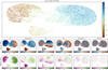 |
Fig. C.1 The C3H2/CH3OH ratio, plotted on the manifold. The manifold is separated into three broad regions. |
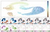 |
Fig. C.2 The HCO/CH3OH ratio, plotted on the manifold. The manifold is a smooth continuous distribution with one separated lobe. |
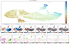 |
Fig. C.3 The CN/HCN ratio, plotted on the manifold. It shows a smooth manifold with a gradient in ratio from top to bottom. |
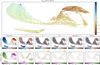 |
Fig. C.4 The HCO+/HCN ratio plotted over a relatively smooth manifold. It shows an elongated manifold with a separate distribution in the lower left corner. |
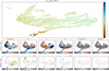 |
Fig. C.5 The HNC/HCN ratio plotted on the manifold. The manifold separates a general region with equal ratio and a lower lobe with HCN enhancement. |
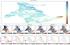 |
Fig. C.6 The CS/SO ratio again shows no clear separation of regions on the manifold. With a tail in the lower right containing SOenhanced models. |
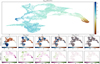 |
Fig. C.7 The SiO/SO ratio plotted on the manifold. It separates into two broad regions, influenced by temperature. |
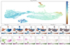 |
Fig. C.8 The CS/CN ratio plotted on the manifold shows a separation between four global regions. |
Appendix D Enumerator and denominator of ratios in density-temperature space
The individual enumerator and denominator of Figure 3 can be found in fig. D.1 and Figure D.2.
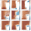 |
Fig. D.1 The enumerator for the ratios as a function of density and temperature including the observational limit. |
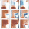 |
Fig. D.2 The denominator for the ratios as a function of density and temperature including the observational limit. |
References
- Akiba, T., Sano, S., Yanase, T., Ohta, T., & Koyama, M. 2019, arXiv e-prints [arXiv:1907.10902] [Google Scholar]
- Arellano-Córdova, K. Z., Esteban, C., García-Rojas, J., et al. 2020, MNRAS, 496, 1051 [Google Scholar]
- Bacmann, A., & Faure, A. 2016, A&A, 587, A130 [NASA ADS] [CrossRef] [EDP Sciences] [Google Scholar]
- Bayet, E., Viti, S., Williams, D. A., & Rawlings, J. M. C. 2008, ApJ, 676, 978 [NASA ADS] [CrossRef] [Google Scholar]
- Bayet, E., Viti, S., Williams, D. A., Rawlings, J. M. C., & Bell, T. 2009, ApJ, 696, 1466 [NASA ADS] [CrossRef] [Google Scholar]
- Bayet, E., Hartquist, T. W., Williams, D. A., et al. 2011, Mem. Soc. Astron. Ital., 82, 893 [Google Scholar]
- Behrens, E., Mangum, J. G., Holdship, J., et al. 2022, ApJ, 939, 119 [NASA ADS] [CrossRef] [Google Scholar]
- Bernal, J. J., Sephus, C. D., & Ziurys, L. M. 2021, ApJ, 922, 106 [NASA ADS] [CrossRef] [Google Scholar]
- Brown, P. D., Charnley, S. B., & Millar, T. J. 1988, MNRAS, 231, 409 [Google Scholar]
- Butterworth, J., Holdship, J., Viti, S., & García-Burillo, S. 2022, A&A, 667, A131 [NASA ADS] [CrossRef] [EDP Sciences] [Google Scholar]
- Chen, T., & Guestrin, C. 2016, in Proceedings of the 22nd ACM SIGKDD International Conference on Knowledge Discovery and Data Mining, 785 [Google Scholar]
- Chen, H., Lundberg, S., & Lee, S.-I. 2019, arXiv e-prints [arXiv:1911.11888] [Google Scholar]
- Chen, B. H., Hashimoto, T., Goto, T., et al. 2022, MNRAS, 509, 1227 [Google Scholar]
- Codella, C., & Bachiller, R. 1999, A&A, 350, 659 [NASA ADS] [Google Scholar]
- Colzi, L., Romano, D., Fontani, F., et al. 2022, A&A, 667, A151 [NASA ADS] [CrossRef] [EDP Sciences] [Google Scholar]
- Esteban, C., Fang, X., García-Rojas, J., & Toribio San Cipriano, L. 2017, MNRAS, 471, 987 [NASA ADS] [CrossRef] [Google Scholar]
- Fontani, F., Colzi, L., Bizzocchi, L., et al. 2022a, A&A, 660, A76 [NASA ADS] [CrossRef] [EDP Sciences] [Google Scholar]
- Fontani, F., Schmiedeke, A., Sánchez-Monge, A., et al. 2022b, A&A, 664, A154 [NASA ADS] [CrossRef] [EDP Sciences] [Google Scholar]
- Fontani, F., Vermariën, G., Viti, S., et al. 2024, A&A, 691, A180 [NASA ADS] [CrossRef] [EDP Sciences] [Google Scholar]
- Gal, R. L., Öberg, K. I., Teague, R., et al. 2021, ApJ Suppl. Ser., 257, 12 [Google Scholar]
- García-Burillo, S., Usero, A., Fuente, A., et al. 2010, A&A, 519, A2 [NASA ADS] [CrossRef] [EDP Sciences] [Google Scholar]
- Grassi, T., Padovani, M., Galli, D., et al. 2025, A&A, submitted [arXiv:2502.07874] [Google Scholar]
- Hacar, A., Bosman, A. D., & Van Dishoeck, E. F. 2020, A&A, 635, A4 [NASA ADS] [CrossRef] [EDP Sciences] [Google Scholar]
- Harada, N., Meier, D. S., Martín, S., et al. 2024a, The ALCHEMI Atlas: Principal Component Analysis Reveals Starburst Evolution in NGC, 253 [Google Scholar]
- Harada, N., Saito, T., Nishimura, Y., Watanabe, Y., & Sakamoto, K. 2024b, arXiv e-prints [arXiv:2405.09029] [Google Scholar]
- Hastie, T., Tibshirani, R., & Friedman, J. 2009, The Elements of Statistical Learning, Springer Series in Statistics (New York, NY: Springer) [CrossRef] [Google Scholar]
- Herbst, E., & van Dishoeck, E. F. 2009, Annu. Rev. A&A, 47, 427 [Google Scholar]
- Heyl, J., Butterworth, J., & Viti, S. 2023a, MNRAS, 526, 404 [Google Scholar]
- Heyl, J., Viti, S., & Vermariën, G. 2023b, Faraday Discuss., 245, 569 [Google Scholar]
- Holdship, J., Viti, S., Jiménez-Serra, I., Makrymallis, A., & Priestley, F. 2017, AJ, 154, 38 [NASA ADS] [CrossRef] [Google Scholar]
- Indriolo, N., Geballe, T. R., Oka, T., & McCall, B. J. 2007, ApJ, 671, 1736 [NASA ADS] [CrossRef] [Google Scholar]
- James, T. A., Viti, S., Yusef-Zadeh, F., Royster, M., & Wardle, M. 2021, ApJ, 916, 69 [NASA ADS] [CrossRef] [Google Scholar]
- Kane, S., Hawkins, K., & Maas, Z. 2023, American Astronomical Society Meeting Abstracts, 241, 208.11 [Google Scholar]
- König, S., Aalto, S., Muller, S., et al. 2018, A&A, 615, A122 [NASA ADS] [CrossRef] [EDP Sciences] [Google Scholar]
- Lamb, K., Malhotra, G., Vlontzos, A., et al. 2019, arXiv e-prints [arXiv:1910.03085] [Google Scholar]
- Li, J., Wang, J., Zhu, Q., Zhang, J., & Li, D. 2015, ApJ, 802, 40 [Google Scholar]
- Lundberg, S., & Lee, S.-I. 2017, arXiv e-prints [arXiv:1705.07874] [Google Scholar]
- Lundberg, S. M., Erion, G., Chen, H., et al. 2020, Nat. Mach. Intell., 2, 56 [CrossRef] [Google Scholar]
- McInnes, L., Healy, J., & Melville, J. 2020, arXiv e-prints [arXiv:1802.03426] [Google Scholar]
- Méndez-Delgado, J. E., Amayo, A., Arellano-Córdova, K. Z., et al. 2022, MNRAS, 510, 4436 [CrossRef] [Google Scholar]
- Milam, S. N., Savage, C., Brewster, M. A., Ziurys, L. M., & Wyckoff, S. 2005, ApJ, 634, 1126 [Google Scholar]
- Millar, T. J., Bennett, A., Rawlings, J. M. C., Brown, P. D., & Charnley, S. B. 1991, A&A Suppl. Ser., 87, 585 [Google Scholar]
- Molnar, C. 2022, Interpretable Machine Learning: A Guide for Making Black Box Models Explainable, 2nd edn. (Munich, Germany: Christoph Molnar) [Google Scholar]
- Pearson, K. 1901, London Edinburgh Dublin Philos. Mag. J. Sci., 2, 559 [CrossRef] [Google Scholar]
- Peñaloza, C. H., Clark, P. C., Glover, S. C. O., & Klessen, R. S. 2018, MNRAS, 475, 1508 [CrossRef] [Google Scholar]
- Ramos, A. A., Plaza, C. W., Navarro-Almaida, D., et al. 2024, MNRAS, 531, 4930 [NASA ADS] [CrossRef] [Google Scholar]
- Ribeiro, M. T., Singh, S., & Guestrin, C. 2016, arXiv e-prints [arXiv:1602.04938] [Google Scholar]
- Rollig, M., Abel, N. P., Bell, T., et al. 2007, A&A, 467, 187 [Google Scholar]
- Ruaud, M., Wakelam, V., & Hersant, F. 2016, MNRAS, 459, 3756 [Google Scholar]
- Sabatini, G., Bovino, S., Giannetti, A., et al. 2021, A&A, 652, A71 [NASA ADS] [CrossRef] [EDP Sciences] [Google Scholar]
- Scholbeck, C. A., Molnar, C., Heumann, C., Bischl, B., & Casalicchio, G. 2019, arXiv e-prints [arXiv:1904.03959] [Google Scholar]
- Semenov, D., Favre, C., Fedele, D., et al. 2018, A&A, 617, A28 [NASA ADS] [CrossRef] [EDP Sciences] [Google Scholar]
- Sewiło, M., Indebetouw, R., Charnley, S. B., et al. 2018, ApJ Lett., 853, L19 [Google Scholar]
- Sewiło, M., Karska, A., Kristensen, L. E., et al. 2022, ApJ, 933, 64 [Google Scholar]
- Shapley, L. S., & Shubik, M. 1971, Int. J. Game Theory, 1, 111 [Google Scholar]
- Shimonishi, T., Izumi, N., Furuya, K., & Yasui, C. 2021, ApJ, 922, 206 [NASA ADS] [CrossRef] [Google Scholar]
- Shimonishi, T., Tanaka, K. E. I., Zhang, Y., & Furuya, K. 2023, ApJ Lett., 946, L41 [Google Scholar]
- Sobol’, I. M. 1967, USSR Computat. Math. Math. Phys., 7, 86 [CrossRef] [Google Scholar]
- Spezzano, S., Caselli, P., Pineda, J. E., et al. 2020, A&A, 643, A60 [NASA ADS] [CrossRef] [EDP Sciences] [Google Scholar]
- Tafalla, M., Usero, A., & Hacar, A. 2021, A&A, 646, A97 [NASA ADS] [CrossRef] [EDP Sciences] [Google Scholar]
- Usero, A., García-Burillo, S., Fuente, A., Martín-Pintado, J., & Rodríguez-Fernández, N. J. 2004, A&A, 419, 897 [NASA ADS] [CrossRef] [EDP Sciences] [Google Scholar]
- van der Maaten, L., & Hinton, G. 2008, J. Mach. Learn. Res., 9, 2579 [Google Scholar]
- Viti, S., & Williams, D. A. 1999, MNRAS, 305, 755 [NASA ADS] [CrossRef] [Google Scholar]
- Wakelam, V., Herbst, E., Le Bourlot, J., et al. 2010, A&A, 517, A21 [NASA ADS] [CrossRef] [EDP Sciences] [Google Scholar]
- Wang, J., Qi, C., Li, S., & Wu, J. 2022, ApJ, 937, 120 [Google Scholar]
- Williams, D. A. 1998, Faraday Discuss., 109, 1 [Google Scholar]
- Wilson, C. D., Bemis, A., Ledger, B., & Klimi, O. 2023, MNRAS, 521, 717 [NASA ADS] [CrossRef] [Google Scholar]
- Woods, P. M., Kelly, G., Viti, S., et al. 2012, ApJ, 750, 19 [NASA ADS] [CrossRef] [Google Scholar]
All Tables
Initial elemental abundances used in UCLCHEM. The number density of hydrogen nuclei is
The ranges for each hyperparameter and the best configuration found after 500 trials with Optuna (Akiba et al. 2019).
All Figures
|
Fig. 1 Fractional abundances for each of the ratios. The contour levels of a kernel density estimate are added to highlight the distribution, each representing 20% of the distribution. For both, we show the observational limit of 10−12 that we used throughout. Only the ratios above either observational threshold were used to train the SHAP explainers. The blue line represents all log-ratios of −12, and the red line represents the log-ratios of 12. |
| In the text | |
|
Fig. 2 Distribution of each of the ratios that exceeded the detection limit for both molecules. The left distribution for each ratio shows where both molecules are detectable, and the right distribution shows this for each molecule where either molecule is detectable. The line in the central box is the median, the central box contains 50% of the ratios, the next upper and lower boxes together contain 25% and so forth, and the outliers plotted as diamonds. |
| In the text | |
|
Fig. 3 Distribution of the log of the ratios as a function of the density and temperature. |
| In the text | |
|
Fig. 4 Relative importance of each physical parameter for all of the ratios. |
| In the text | |
|
Fig. 5 All of the SHAP values for each of the ratios. The features are sorted by mean absolute impact as shown in Figure 4. Every color map is normalized to the detectable range for each individual feature per ratio. |
| In the text | |
|
Fig. 6 H2CO/CH3OH ratio, feature, and SHAP values plotted on a two-dimensional manifold using the ratio and the SHAP values. The manifold consists of a broad left region with two separate right lobes. |
| In the text | |
|
Fig. C.1 The C3H2/CH3OH ratio, plotted on the manifold. The manifold is separated into three broad regions. |
| In the text | |
|
Fig. C.2 The HCO/CH3OH ratio, plotted on the manifold. The manifold is a smooth continuous distribution with one separated lobe. |
| In the text | |
|
Fig. C.3 The CN/HCN ratio, plotted on the manifold. It shows a smooth manifold with a gradient in ratio from top to bottom. |
| In the text | |
|
Fig. C.4 The HCO+/HCN ratio plotted over a relatively smooth manifold. It shows an elongated manifold with a separate distribution in the lower left corner. |
| In the text | |
|
Fig. C.5 The HNC/HCN ratio plotted on the manifold. The manifold separates a general region with equal ratio and a lower lobe with HCN enhancement. |
| In the text | |
|
Fig. C.6 The CS/SO ratio again shows no clear separation of regions on the manifold. With a tail in the lower right containing SOenhanced models. |
| In the text | |
|
Fig. C.7 The SiO/SO ratio plotted on the manifold. It separates into two broad regions, influenced by temperature. |
| In the text | |
|
Fig. C.8 The CS/CN ratio plotted on the manifold shows a separation between four global regions. |
| In the text | |
|
Fig. D.1 The enumerator for the ratios as a function of density and temperature including the observational limit. |
| In the text | |
|
Fig. D.2 The denominator for the ratios as a function of density and temperature including the observational limit. |
| In the text | |
Current usage metrics show cumulative count of Article Views (full-text article views including HTML views, PDF and ePub downloads, according to the available data) and Abstracts Views on Vision4Press platform.
Data correspond to usage on the plateform after 2015. The current usage metrics is available 48-96 hours after online publication and is updated daily on week days.
Initial download of the metrics may take a while.