| Issue |
A&A
Volume 697, May 2025
|
|
|---|---|---|
| Article Number | A88 | |
| Number of page(s) | 16 | |
| Section | Extragalactic astronomy | |
| DOI | https://doi.org/10.1051/0004-6361/202347102 | |
| Published online | 08 May 2025 | |
JADES: Differing assembly histories of galaxies
Observational evidence for bursty star formation histories and (mini-)quenching in the first billion years of the Universe
1
Kavli Institute for Cosmology, University of Cambridge, Madingley Road, Cambridge CB3 0HA, UK
2
Cavendish Laboratory, University of Cambridge, 19 JJ Thomson Avenue, Cambridge CB3 0HE, UK
3
Department of Physics and Astronomy, University College London, Gower Street, London WC1E 6BT, UK
4
European Southern Observatory, Karl-Schwarzschild-Strasse 2, D-85748 Garching bei Muenchen, Germany
5
Centro de Astrobiología (CAB), CSIC-INTA, Cra. de Ajalvir Km. 4, 28850 Torrejón de Ardoz, Madrid, Spain
6
Department of Physics and Astronomy, University of Manitoba, Winnipeg, MB R3T 2N2, Canada
7
Cosmic Dawn Center (DAWN), Copenhagen, Denmark
8
Niels Bohr Institute, University of Copenhagen, Jagtvej 128, DK-2200 Copenhagen, Denmark
9
Steward Observatory University of Arizona, 933 N. Cherry Avenue, Tucson, AZ 85721, USA
10
School of Physics, University of Melbourne, Parkville, 3010 VIC, Australia
11
ARC Centre of Excellence for All Sky Astrophysics in 3 Dimensions (ASTRO 3D), Canberra, Australia
12
Department of Physics, University of Oxford, Denys Wilkinson Building, Keble Road, Oxford OX1 3RH, UK
13
Scuola Normale Superiore, Piazza dei Cavalieri 7, I-56126 Pisa, Italy
14
Sorbonne Université, CNRS, UMR 7095, Institut d’Astrophysique de Paris, 98 bis bd Arago, 75014 Paris, France
15
Centre for Astrophysics Research, Department of Physics, Astronomy and Mathematics, University of Hertfordshire, Hatfield AL10 9AB, UK
16
Center for Astrophysics | Harvard & Smithsonian, 60 Garden St., Cambridge, MA 02138, USA
17
Max-Planck-Institut für Astronomie, Königstuhl 17, D-69117 Heidelberg, Germany
18
AURA for European Space Agency, Space Telescope Science Institute, 3700 San Martin Drive, Baltimore, MD 21210, USA
19
Department for Astrophysical and Planetary Science, University of Colorado, Boulder, CO 80309, USA
20
Department of Astronomy and Astrophysics University of California, Santa Cruz, 1156 High Street, Santa Cruz CA 96054, USA
21
Astrophysics Research Institute, Liverpool John Moores University, 146 Brownlow Hill, Liverpool L3 5RF, UK
22
NSF’s National Optical-Infrared Astronomy Research Laboratory, 950 North Cherry Avenue, Tucson, AZ 85719, USA
23
NRC Herzberg, 5071 West Saanich Rd, Victoria, BC V9E 2E7, Canada
⋆ Corresponding author: This email address is being protected from spambots. You need JavaScript enabled to view it.
Received:
5
June
2023
Accepted:
22
December
2024
Abstract
We used deep NIRSpec spectroscopic data from the JADES survey to derive the star formation histories (SFHs) of a sample of 200 galaxies at 0.6 < z < 11 that span stellar masses from 106 to 109.5 M⊙. We found that galaxies at high redshift, galaxies above the main sequence (MS), and low-mass galaxies tend to host younger stellar populations than their lower-redshift, below the MS, and more massive counterparts. Interestingly, the correlation between age, stellar mass M*, and star formation rate (SFR) existed even earlier than cosmic noon, out to the earliest cosmic epochs. However, these trends have a large scatter. There are also examples of young stellar populations below the MS, which indicates recent (bursty) star formation in evolved systems. We further explored the burstiness of the SFHs by using the ratio of the SFR averaged over the last 10 Myr and averaged between 10 Myr and 100 Myr before the epoch of observation (SFRcont, 10/SFRcont, 90). We found that high-redshift and low-mass galaxies have particularly bursty SFHs, while more massive and lower-redshift systems evolve more steadily. We also present the discovery of another (mini-)quenched galaxy at z = 4.4, which might be only temporarily quiescent as a consequence of the extremely bursty evolution. Finally, we also found a steady decline in the dust reddening of the stellar population as the earliest cosmic epochs are approached, although some dust reddening is still observed in some of the highest-redshift and most strongly star-forming systems.
Key words: galaxies: evolution / galaxies: formation / galaxies: high-redshift / galaxies: starburst / galaxies: star formation
© The Authors 2025
 Open Access article, published by EDP Sciences, under the terms of the Creative Commons Attribution License (https://creativecommons.org/licenses/by/4.0), which permits unrestricted use, distribution, and reproduction in any medium, provided the original work is properly cited.
This article is published in open access under the Subscribe to Open model. This email address is being protected from spambots. You need JavaScript enabled to view it. to support open access publication.
1. Introduction
A key objective in modern astrophysics is understanding the nature and characteristics of stellar populations and the assembly histories of their host galaxies. Stellar populations offer a unique window into the early Universe and provide insights into the formation and evolution of galaxies.
The launch of the James Webb Space Telescope (JWST, Gardner et al. 2006, 2023) with its unparalleled capabilities ushered in a new era of astronomical exploration. The telescope provides the opportunity of uncovering the intricate characteristics of stellar populations in objects at redshifts that previously were unattainable. The spectroscopic capabilities of the Near Infrared Spectrograph (NIRSpec, Jakobsen et al. 2022) on board the JWST and its high sensitivity enable us to push to fainter sources which have lower masses or are more distant and to measure their properties accurately. With the JWST, we can explore the early stages of galaxy formation and trace the evolution of stellar populations across cosmic time.
Stellar populations are a crucial tool for understanding the assembly of galaxies because their past star formation histories (SFHs) are imprinted in their stellar record. Hence, they encode valuable information about the various physical mechanisms that shaped their past star formation activity, such as stellar winds, feedback from supernovae (SN) and active galactic nuclei (AGN), interactions and mergers, or the environment.
It is now widely thought, as predicted by numerical simulations (Kawata & Gibson 2003; Ceverino et al. 2021; Dome et al. 2024) and emerging observational evidence (Glazebrook et al. 1999; Caputi et al. 2007; Smit et al. 2014, 2015; Díaz-Santos et al. 2017; Endsley et al. 2021, 2024, 2023; Whitler et al. 2023), that these mechanisms can cause the SFHs to become bursty, in particular, in the early Universe (Faucher-Giguère 2018; Tacchella et al. 2016) and in low-mass systems (Weisz et al. 2012; Tacchella et al. 2020). Here, “burstiness” refers to patterns of star formation that are characterized by episodic bursts of intense activity, interspersed with lull phases. In these phases, the galaxy is forming significantly fewer stars at the epoch of observation (timescale of ∼10 Myr) than during its recent past (timescale of ∼100 Myr), and potentially even quiescent periods, so-called mini-quenching events (Dome et al. 2024; Gelli et al. 2023). Mini-quenching events refer to the state of a galaxy in which star formation is temporarily halted or strongly suppressed, that is, the specific star formation rate (sSFR) of the galaxy satisfies sSFR < 0.2/tobs, likely because the inflow of gas into the galaxy is disrupted. This temporarily halts the star formation activity. Unlike long-term quenching processes that lead to a permanent decline in star formation, mini-quenching events are transient and typically only last for a few tens to one hundred million years.
It is therefore crucial to study bursty SFHs and mini-quenching for our understanding of the diversity of galaxy properties and the underlying physical processes that shape them. The timing, duration, and intensity of star formation bursts can influence the overall stellar mass assembly, the enrichment of heavy elements, and the morphological evolution of galaxies. Furthermore, bursty SFHs are likely connected to the growth of supermassive black holes and the feedback mechanisms associated with AGN, even in low-mass systems Koudmani et al. (2019). Hence, the investigation of the burstiness in galaxy SFHs provides important constraints for theoretical models. It is also essential for constructing a comprehensive picture of galaxy evolution and unraveling the intricate processes that drive the diverse ranges of galaxy properties observed in the Universe.
Nevertheless, although it is thought to be a common phenomenon in galaxy evolution, observational evidence for bursty SFHs and mini-quenching is still sparse to date, mainly because of the limitations of pre-JWST instruments. Early results with JWST on SFHs at high redshift were unable to prove the presence of bursty SFHs unambiguously. Dressler et al. (2023) showed evidence for a bursty evolution through interrupted star formation as a function of lookback time for half their sample of 24 galaxies. The sample was observed with seven NIRCam wide- and medium-band filters. The results also held for a variety of other types of histories, ranging from semicontinuous “runs of star formation over contiguous epochs” with periods of intermission between the individual runs to extended continuous star formation. This result was later confirmed with a larger galaxy sample (Dressler et al. 2024).
However, spectra with a high signal-to-noise ratio are required to identify and characterize bursty SFHs on shorter timescales (within the last 100 Myr before the epoch of observation) and to breaking the degeneracies between different possible SFHs. These spectra allow us to (i) unambiguously separate the flux from nebular emission lines from the flux that arises from the stellar continuum, (ii) mitigate the effect of outshining, and (iii) disentangle the recent star formation history of a galaxy.
The study of the burstiness and mini-quenching at high redshift is further complicated by the fact that, observationally, we (obviously) cannot know the future of any particular galaxy. Hence, it is difficult to assess on which timescales, if not permanently, a particular quenched galaxy remains quenched. This makes it difficult observationally to differentiate between mini-quenching and permanent quenching on a galaxy-by-galaxy basis. However, data on molecular cold gas in or around the galaxy, or evidence for infalling giant clouds of cold gas, might give us important clues on whether the galaxy will obtain new fuel for star formation in the near future. Hence, unless this information is available for any particular galaxy we observe in a quiescent phase, we can only speculate about the duration over which the galaxy remains quenched. We therefore propose to call these objects (mini-)quenched to indicate that it is likely that they will reignite again in the future, in particular, for high-redshift or low-mass systems. We also admit the possibility that they continue to have a very low sSFR over extended timescales, however, or that they remain permanently quenched.
In order to unambiguously establish mini-quenching observationally, rejuvenating galaxies have yet to be observed. These are characterized by old stellar populations and a UV faintness and simultaneous show strong nebular emission lines that trace recent star formation. Additionally, more galaxy spectra are needed to identify galaxies in different phases of their burstiness cycles: from bursts to regular to lull phases (see, e.g., the post-starburst nearly quiescent galaxy in Strait et al. 2023) to mini-quenching and to rejuvenating galaxies so that we can provide constraints on the physical processes that shape the burstiness of SFHs. Until large data sets like these are obtained, we propose to call these types of quiescent galaxy that might soon reignite again in the future such as the one presented in Looser et al. (2024a) (mini-)quenched, as argued above.
Large statistical samples are needed to characterize burstiness, (mini-)quenching events, and the associated duty cycles as a function of different galaxy population properties, such as observed redshift, stellar mass M⋆, or the distance from the main sequence (MS).1 This leaves the burstiness of high-redshift and low-mass galaxies and the physics that shapes it as one of the major unknowns in galaxy assembly and evolution to date, and one of the key science goals for the JWST.
We present a detailed study of stellar populations in high-redshift galaxies and observational results on the burstiness of SFHs as a function of stellar mass and redshift. We also report observational evidence for (mini-)quenching events at high redshift. This work is based on data acquired by our JWST Advanced Deep Extragalactic Survey (JADES; Eisenstein et al. 2023) survey. JADES is a large JWST GTO program that was formed out of a collaboration between the NIRSpec (Jakobsen et al. 2022) and NIRCam (Rieke et al. 2023) instrument science teams, which combines imaging and spectroscopy. The program is designed to present an unprecedented study of the physical properties of galaxies at high redshift, and it mostly focuses on targets beyond cosmic noon.
The paper is structured as follows: In Section 2 we present our JADES data, in particular, the NIRSpec PRISM spectra, we summarize the data processing and describe our full spectral fitting method, which is based on PPXF (Cappellari 2017, 2023). In Section 3 we discuss our observational results for the stellar ages and stellar dust attenuation in different bins of characteristic galaxy properties. In Section 4 we present our results on the burstiness of SFHs. In Section 5 we discuss our results. In Section 6 we summarize the key findings of this paper.
Throughout this work, we assume a Chabrier (Chabrier 2003) initial mass function (IMF) and aΛCDM cosmology with the following parameters: H0 = 70 km s−1/Mpc, ΩM = 0.3, and ΩΛ = 0.7.
2. Data, data reduction, and extraction of the basic physical quantities
The NIRSpec (Jakobsen et al. 2022) micro-shutter array (MSA, Ferruit et al. 2022) spectra used in this work were obtained as part of our JADES GTO program (PI: N. Lützgendorf, ID:1210) observations in the Great Observatories Origins Deep Survey South field (GOODS-S; Giavalisco et al. 2004) between October 21–25, 2022. These spectra form the deep tier of our survey which targeted galaxies preselected using the Hubble Space Telescope (HST) (hereafter referred to as JADES/HST-DEEP). These were obtained using the PRISM configuration, which covers the wavelength range between 0.6 μm and 5.3 μm and provides spectra with a nominal wavelength-dependent spectral resolution of R ∼ 30 − 330 (Jakobsen et al. 2022)2.
The program observed a total of 253 galaxies over three dithering pointings. For each target, three microshutters were opened simultaneously for exposure. The exposure time per target ranged from 9.3 to 28 hours, depending on whether a target was observed at all three, at two, or at only one dither pointing. Each dither pointing consisted of four sequences of three-nod patterns along the slit. The observation time for each three-nod pattern was 8403 seconds, resulting in an integration time for each dither pointing of 33 612 seconds (= 9.3 hours). Each dither pointing used a different MSA configuration to place the spectra at different positions on the detector, to decrease the impact of detector gaps, mitigate detector artifacts, and improve the signal-to-noise ratio (S/N) for high-priority targets, while increasing the density of the observed targets.
The flux-calibrated spectra were extracted using pipelines developed by the ESA NIRSpec Science Operations Team (SOT) and the NIRSpec GTO Team. A detailed description of the pipelines will be presented in a forthcoming NIRSpec/GTO collaboration paper (Carniani et al., in prep.). For a more detailed presentation of the JADES/HST-DEEP spectra and a discussion of the sample selection, we refer to Bunker et al. (2024). In this paper, we use all spectra for which a redshift could be established. For galaxies with strong emission lines, we used the same redshifts as were presented in Bunker et al. (2024). Otherwise, we used redshifts inferred from visual inspection of the continuum and weaker lines, which were further refined by PPXF (see below).
We remark that with the effective slit width of 0.2 arcsec, the JADES spectra suffer from wavelength-dependent aperture losses. This was corrected assuming a point-source geometry, which led to a systematic underestimate of the flux for the most extended lowest-redshift sources.
2.1. Full spectral fitting with PPXF
The R100 spectra were fit with a method that is based on the χ2-minimization penalized PiXel-fitting code3 PPXF (Cappellari 2017, 2023), using bootstrapping to infer key physical quantities (Looser et al. 2024b). To fit the stellar continuum, a library of simple stellar population (SSP) templates was fit as a (non-negative) linear superposition to the continuum spectrum. The SSP library uses synthetic model atmospheres from the C3K library (Conroy et al. 2019) with a resolution of R = 10 000, adopting the MIST isochrones of Choi et al. (2016), solar abundances, and a Salpeter IMF4. The SSP templates were all multiplicatively coupled to the same Calzetti et al. (2000) dust attenuation curve, adopting E(B-V) as one free parameter (but without any additive or multiplicative polynomials). Throughout the paper, we changed the IMF to Chabrier using the formula of Speagle et al. (2014): M*, C = 0.58 M*, S, with C and S referring to the Chabrier and Salpeter IMFs, respectively. The synthetic SSP spectra span the 2D age-metallicity logarithmic grid from ageSSP = 106.0 yr to 1010.3 yr and [M/H] = –2.5 to 0.5. For each galaxy, we cut the age grid to be consistent with the age of the Universe at this redshift, plus a buffer of at least 0.1 dex and 0.2 dex at most, that is, either one or two age bins. In other words, we allowed the galaxy to be 26–58% older than the age of the Universe at this redshift (see McDermid et al. (2015), for a discussion). For a self-consistent treatment of the nebular emission lines, we used Gaussians to fit them simultaneously with the stellar continuum. The SSP models themselves do not include nebular emission.
In the following, we describe the method based on the PPXF algorithm in detail that we applied to each JADES/HST-DEEP spectrum in this work.
-
First, the C3K templates were convolved to match the wavelength-dependent spectral resolution of the spectrum. Secondary to the wavelength, the effective spectral resolution (R) depends on the degree of slit filling, that is, the ratio of the galaxy size and the 0.2 arcsec width of the microshutters. This effect was estimated to be as large as a factor of two. Because PPXF can compensate for an overestimated R (with kinematic broadening) but cannot compensate for an underestimated R, we conservatively increased R for all targets by a factor 1.7. This factor was derived purely phenomenologically from the observed width of the emission lines in the sample.
-
The spectrum and templates were renormalized by the median flux per spectral pixel in the spectrum to avoid numerical issues and to enable the use of regularization in PPXF (‘regul’ keyword). This allowed us to penalize nonsmooth weight distributions (see Cappellari 2017 for more details).
-
A first fit with regul = 5 was used to obtain an initial estimate of the model and to remove outliers using a 4σ clipping.
-
We then performed a wild bootstrapping by perturbing the spectrum S with the estimated noise spectrum from the data reduction N: S*(λ) = S(λ)±N(λ′), where N(λ′) was chosen randomly from the noise spectrum within ±50 pixels for each spectral pixel λ.
-
We fit the perturbed spectrum S*(λ) again with PPXF, again with regul = 5.
-
Steps 4 and 5 were repeated 100 times.
-
This method probes the sampling distribution of each individual SSP grid weight. The 100 bootstrapped grids of SSP weights were then averaged to recover a nonparametric SFH consistent with the intrinsic noise of the spectrum.
The output is a reconstructed assembly history of the target under consideration, as traced by this archaeological approach, using the observed remaining stellar populations as the fossil record of the system. Because we assumed point sources in the data reduction, our spectra do not capture the absolute M⋆ and SFR of each galaxy and lead to values that are systematically underestimated. In addition, by modeling the spectra alone (i.e., without photometry), we neglect any light falling outside the MSA shutters; in particular, no color gradients and clumpy morphologies can be captured by our approach. However, we remark that the impact of this effect is strongest where it is least relevant to our conclusions, that is, in the lowest-redshift bin and at the highest stellar masses.
The distinctive advantage of our approach is that by fitting the observed spectra with a superposition of independent SSPs and gas templates, we did not impose a particular parametric SFH or a single metallicity on the spectrum. In other words, our recovered SFHs are nonparametric and do not depend on any assumption about the underlying physics of the galaxy evolution. Crucially, any recovered scaling relation cannot have been introduced by parametric assumptions about the shape of our fitted SFHs. As an example, the light-weighted 2D fitted grid of SSP weights and the conversion of these weights into a nonparametric SFH for the spectra presented in Fig. 1 is shown in Figs. A.1 and A.2.
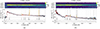 |
Fig. 1. Examples of JADES/HST-DEEP spectra at high redshift. The fitted PPXF continuum is shown in red, and the nebular emission lines are shown in yellow. The bottom panel indicates the reduced residuals of the fits The vertical dashed lines mark the rest-frame wavelengths of strong nebular emission lines. The noise is indicated by the shaded blue regions. The upper panel shows the S/N of the combined 2D spectrum (the 1D spectrum was not extracted from the combined 2D spectrum). Left: A star-bursting galaxy at redshift z = 5.9 that might be rejuvenating. We note the simultaneous presence of (i) a Balmer break and a shallow β-slope, and (ii) strong nebular emission lines. Right: A weakly star-forming galaxy at redshift z = 3.6. We note the simultaneous presence of (i) a strong Balmer break and a shallow β-slope, and (ii) weak nebular emission lines. |
While this nonparametric astro-archaeological approach is extremely powerful, its outputs have to be analyzed with care. This method was tested on data from the local MaNGA (Bundy et al. 2015) survey and was shown to recover meaningful average star formation and chemical evolution histories (Looser et al. 2024b).
While the recovered ages traced by the UV-slope, the Balmer break, and the overall shape of the spectrum can be recovered reliably, the spectral resolution of the NIRSpec PRISM spectra may not be sufficient to reliably estimate the metallicity of the underlying galaxy populations. The well-known age-metallicity degeneracy and the known and unknown systematics such as dust obscuration or flux calibration issues mean that we can trust the returned SSP weights to different degrees. To assess the stability of the SSP weights, the bootstrapping method described above is highly instructive because it returns a scatter distribution for each individual SSP weight and also for any quantity derived from the weight grid. The tests revealed that ages are reliable in conservative 1 dex bins in log10(Age [yr]), from log10(Age [yr]) = 6.0–10.0. For this paper, we therefore bin the SSP weight-grid as presented in Fig. A.2 into four age bins as presented below (see Figs. 3–5).
2.2. Stellar mass
To measure the stellar mass M⋆ for each galaxy, we summed the individual weights of the mass-weighted SSP grid inferred with PPXF. To test the reliability of the PPXF masses, we compared them to the masses inferred from the code BEAGLE (Chevallard & Charlot 2016) for the same data set, as presented in Curti et al. (2024) and Chevallard et al. (in prep.). The PPXF masses and the BEAGLE masses show a strong correlation with an RMS scatter of 0.2 dex, but we note an offset of 0.2 dex. Even though the two codes infer different masses for some galaxies, the general agreement means that our choice of M⋆ does not drive the results presented in this paper. A comparison between the PPXF and BEAGLE masses is presented in Appendix B.
2.3. SFR from nebular Balmer lines
To calculate the SFR from nebular emission lines, we followed a similar method as Curti et al. (2024). We applied the calibration of Kennicutt & Evans (2012), using the attenuation-corrected Hα luminosity where available, that is, at z ≲ 7, and 2.86 × Hβ otherwise. The dust-attenuation correction was either based on the Balmer decrement (Hα/Hβ = 2.86 or Hβ/Hγ = 0.47; where both lines are detected) adopting a Gordon et al. (2003) dust correction, or on the E(B-V) from a full spectral fitting, where only one Balmer line was detected.
Fig. 2 shows the SFR-mass plane in three different redshift bins. The blue lines represent simple linear fits to the SFR–M⋆ relation for this particular sample in the three redshift ranges. The fit likely overestimates the true normalization of the MS because of complex selection effects. The main reason is probably the observability bias; low-SFR faint targets are not bright enough to be observed with NIRSpec, even with the long exposure times used in JADES, and hence are not represented in this sample. However, literature estimates that were derived from shallower data are likely to be even more strongly affected by this phenomenon. The adopted observation strategy based on different target priority classes and the resulting slit allocation in the MSA for JADES/HST-DEEP might play an additional secondary role as well.
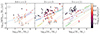 |
Fig. 2. SFR-mass plane, color-coded by the average mass-weighted stellar ages measured by PPXF in three different redshift bins. Each data point represents a single galaxy. The blue lines represent a simple linear fit to the SFR–M⋆ relation of this sample in that redshift bin. For reference, various observational MS estimates (Santini et al. 2017; Popesso et al. 2023; Rinaldi et al. 2022) and predictions from simulations (Ma et al. 2018; Yung et al. 2019) are presented, as indicated by the labels. We extrapolated these MS by ca. 0.5 dex in stellar mass where necessary to compare them to our lower-mass sample. The three dotted lines indicate the quenched threshold for the same redshifts (see main text). The error bar in the upper left corner represents the RMS errors for M⋆ and SFR for the entire sample. Quiescent and (mini-)quenched galaxies and other galaxies for which no SFR could be estimated because the relevant nebular emission lines were not detected are plotted with upper limits. |
Toward the high-mass end of our dataset, at log10(M⋆) = 8.0 − 9.0, where our stellar masses overlap with previous observational estimates (e.g., Popesso et al. 2023; Laporte et al. 2023; Rinaldi et al. 2022; Bisigello et al. 2018; Santini et al. 2017), our MS estimate broadly aligns with the literature. However, at lower masses, our sample lies above the extrapolated literature MS estimates, likely due to observational bias. This effect is most pronounced in the high-redshift bin, providing further evidence of observational bias in our sample.
As this work is based on one of the deepest data sets obtained with the JWST to date, our observations focused on fainter objects with lower masses than earlier observational studies. A comparison to the MS from simulations (Ma et al. 2018; Yung et al. 2019) again suggests that despite our higher sensitivity, we still overestimate the average SFR of the MS.
Part of the observed scatter around the MS might be due to the evolution of the sSFR within the large redshift bins we used, which were necessitated by the limited sample size. A more careful analysis of the MS would require a larger sample and accounting for selection bias and redshift-binning effects, but this is beyond the scope of this work. For the lowest, middle, and highest redshift in each of the three redshifts bin, we plot the redshift-dependent quenching threshold sSFR < 0.2/tobs, where tobs(z) is the age of the Universe as a function of redshift (e.g. Gallazzi et al. 2014; Pacifici et al. 2016; Carnall et al. 2023). The quenching-threshold redshifts are z = 0, 1, 2 for the lowest redshift bin (plotted in orange, green, and red, respectively); z = 2, 3.5, 5 for the middle redshift bin; and z = 5, 8, 11 for the highest redshift bin.
3. Results: Stellar populations
In this section, we present the results of our nonparametric full spectral fitting with PPXF on the inferred stellar population properties.
3.1. Stellar ages as a function of M⋆, ΔMS, and redshift z
In Fig. 2, individual galaxies are color-coded by their mass-weighted stellar ages. As expected, the average ages of the galaxies decrease with increasing redshift. Furthermore, we observe interesting trends with M⋆ and ΔMS: (a) High-mass galaxies tend to be older overall than low-mass galaxies in all redshift bins (in agreement with recent studies at cosmic noon; e.g., Carnall et al. 2019a; Tacchella et al. 2022; Ji & Giavalisco 2022), although there is considerable variation; (b) at fixed stellar mass, galaxies above the MS (as traced by nebular emission lines on timescales of 10 Myr) are younger than galaxies below the MS. This indicates that the ΔMS of a galaxy at the epoch of observation is correlated to some extent with its past formation history over longer timescales. However, there is significant variation. The interesting question is whether this is due to measurement uncertainties or bursty SFHs, as we discuss below.
3.2. Stacked SFHs
In Figs. 3–5 the SFHs of individual galaxies are combined together to provide a composite view. The individual SFHs are stacked in three z, M⋆, and ΔMS bins, as indicated by the labels. We reiterate that the individual PPXF SSP-grid fits are nonparametric: PPXF can freely choose the weighting of each individual SSP spectrum given, without any assumption on the functional form of the SFH. The stacks in each bin were constructed as follows. First, we normalized for each galaxy the SSP weights by the total sum of SSP-weights, that is, we constructed a “relative” weight-distribution of SSPs. These normalized weights were then averaged (i.e., each galaxy contributed equally) over all galaxies in a given z–M⋆–ΔMS bin. The inferred SSP-weight grids were then averaged over four log-age bins with a width of 1 dex. This facilitated the identification of relative trends, and our bootstrapping tests indicate that the inferred grid weights are not reliable on a finer age sampling.
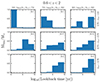 |
Fig. 3. Mass-weighted stacks of normalized SFHs of galaxies in three bins each of M⋆ and ΔMS in the redshift range 0 < z < 2. The number in the legend of each panel indicates the number of galaxies that contribute to the stack. In each bin, the SSP weights of each contributing galaxy are first normalized and then averaged over all galaxies that contribute to the bin. The underlying inferred SSP weight-grid is collapsed into four age bins, where each bin has a width of 1 dex, as indicated. For each individual galaxy SFH, the age-cutoff of the SSP templates depends on the redshift of the target and is 0.1 dex at least and 0.2 dex at most, i.e., either one or two age bins, older than the age of the Universe at that redshift (see McDermid et al. 2015, for a discussion). The 1 dex age-bin weights are then calculated from the sum over all galaxies and over all their weights falling into that age bin (see Section 2.1 for more details). |
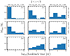 |
Fig. 4. Mass-weighted stacks of normalized SFHs of galaxies in three M⋆ and ΔMS bins in the redshift bin 2 < z < 5. The number in the legend of each panel indicates the number of galaxies that contribute to each stack (see Fig. 3 and Section 2.1 for more details). |
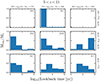 |
Fig. 5. Mass-weighted stacks of individual normalized SFHs of galaxies in three M⋆ and ΔMS bins for galaxies with redshifts z > 5. The number in the legend of each panel indicates the number of galaxies that contribute to the stack (see Fig. 3 and Section 2.1 for more details). |
The stacked SFHs revealed interesting patterns in the SFHs of different galaxy populations in the sample as a function of z, M⋆, and ΔMS, similar to those found for more massive galaxies around cosmic noon (Ji & Giavalisco 2023). As expected, low-redshift galaxies exhibit older populations, and more stellar mass is formed at long look-back times. Conversely, high-redshift galaxies are mostly dominated by young stellar populations. Within each redshift bin, there are also interesting trends with ΔMS and M⋆: Galaxies below the MS tend to have a significantly greater contribution of old SSPs than galaxies on the MS, whereas galaxies above the MS exhibit the highest mass fraction of young SSPs. Additionally, there is a weak trend with M⋆: Massive galaxies tend to be older than low-mass galaxies.
However, a very interesting finding is that evolved (old) stellar populations (that formed more than one Gyr before the epoch of observation) substantially contribute even in the highest redshift bin. This indicates that the SFH analysis reveales the imprint of the earliest episodes of star formation in these systems. However, we caution that it is quite difficult to infer the oldest stellar populations in these systems because they contribute little to the stellar light. This finding should therefore be confirmed with additional data.
3.3. Dust attenuation as a function of M⋆, ΔMS, and redshift z
Fig. 6 shows the SFR mass planes color-coded by E(B-V), which traces the amount of reddening in the stellar continuum that is caused by interstellar dust along the line of sight. E(B-V) was fit for with PPXF assuming the Calzetti et al. (2000) dust attenuation law. The galaxies are divided into the same three redshift bins as in Section 3.1. The trend with ΔMS is clear: Spectra of quiescent galaxies and galaxies below the MS show a weaker dust attenuation, while particularly star-bursting galaxies exhibit significant reddening (see also Sandles et al. 2024). Additionally, there is a trend with M⋆: Massive galaxies tend to be dustier than low-mass galaxies. Finally, the dust reddening declines at the highest redshift (at a given stellar mass and SFR), although most galaxies in the highest-redshift bins still show some but moderate amounts of dust, especially in the more strongly star-forming and higher-mass systems. In the two lower-redshift bins, most galaxies below the MS exhibit no dust at all, while particularly high-mass star-bursting galaxies above the MS show significant dust reddening of the stellar continuum. Overall, the mass dependence observed in the local Universe and at low redshift is recovered (e.g., Pannella et al. 2009; Whitaker et al. 2017; McLure et al. 2018; Shapley et al. 2022; Maheson et al. 2024), but with a clear dependence on the SFH and/or redshift.
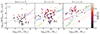 |
Fig. 6. SFR mass plane color-coded by reddening E(B-V) of the stellar populations, inferred with a PPXF fitting of stellar populations convolved with a Calzetti et al. (1994) dust attenuation law with E(B-V) as a free parameter in three different redshift bins. Each data point represents a single galaxy. The galaxies for which no SFR could be measured are plotted with upper limits. Some are below the quenching threshold and clearly quiescent, while some residual star formation cannot be ruled out for others. More details are given in Fig. 2. |
3.4. SFR from stellar populations
In Fig. 7 we present the results from the direct inference of the SFRcont over different timescales from the stellar populations and compare this to the SFR estimated from nebular emission lines (SFRneb, 10) (see Section 2.3), where the SFRcont was derived via fitting the stellar continuum with PPXF; and averaged over 10 Myr (SFRcont, 10, left) and 100 Myr (SFRcont, 100, right), respectively.
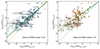 |
Fig. 7. SFR measured from nebular emission lines that trace the SFR over timescales of ∼10 Myr using the K12 relation (y-axis; see Section 2.3 for more details) vs. SFR measured from the nonparametric stellar population fit of the continuum with PPXF (x-axis). Left: SFR estimated from stellar population fitting with PPXF averaged over the last 10 Myr before the observations. The RMS scatter between the two measurements is 0.3 dex, and we note an offset of 0.2 dex (see text). Right: SFR estimated from stellar population fitting with PPXF averaged over 100 Myr before the observations. |
SFRcont, 10 traced by the stellar continuum and SFRneb, 10 traced by the optical Balmer lines agree very well. The small difference in normalization might partially be explained by the assumption of solar metallicity in K12, which overestimates the SFR in metal-poor systems. A comparison between K12 and a metallicity-calibrated SFR, see, for instance, Shapley et al. (2023), will be presented in a forthcoming work. For this study, we focused on the mean trend and its scatter, and we therefore ignored the systematic offset.
The right panel of Fig. 7 shows a strong correlation between SFRcont, 100 and SFRneb, 10, although there is more scatter, and the normalization deviates.
The interesting question is how much of the scatter and offset between these two quantities stems from noise and measurement uncertainty, and how much comes from (i) physical variability in SFR, that is, bursty SFHs, and (ii) selection bias that is, we preferentially observe galaxies in star-bursting phases because they are much brighter in the nebular emission line luminosities and UV continuum luminosity (see Sun et al. 2023, for a more detailed discussion).
We present observational evidence in the next section that a significant part of the scatter is physical, which indicates bursty SFHs in particular in high-redshift and low-mass systems.
4. Results: Observational evidence for bursty SFHs
In this section, we present observational results that indicate bursty SFHs in high-redshift and low-mass systems. Specifically, in addition to the star-bursting galaxy in Fig. 1a, we show examples of galaxies in regular phases, that is, galaxies that formed stars at roughly the same rate over the last 10 Myr as over the last 100 Myr; and galaxies in lull phases, that is, galaxies that formed significantly fewer stars over the last 10 Myr relative to the last 100 Myr, but with detected Balmer lines that are associated with recent star formation activity and above the quenched threshold (sSFR ≳ 0.2/tobs). More broadly, we present an analysis of burstiness as a function of redshift z and in the SFR mass plane. Furthermore, we present the discovery of an additional low-mass (mini-)quenched galaxy in a quiescent phase at high redshift. Finally, we also discuss observational biases.
4.1. Examples of galaxies in lull or regular phases at high-z
Fig. 8 shows two examples of observed JADES/HST-DEEP galaxies in a lull and a regular phase, respectively, in the intermediate-redshift bin. Although both spectra are blue with a steep UV slope, which indicates strong star formation over the past ∼100 Myr, the nebular emission lines in Fig. 8a are low luminosity, which indicates lower star formation activity over the last ∼10 Myr before the epoch of observation. The nebular emission lines in Fig. 8b indicate regular star-formation activity over the last 10 Myr. The regular galaxy shows low EW emission in Hβ, [OIII], and Hα for these redshifts. The lulling galaxy shows an even lower EW, particularly in Hα, and no detection of Hβ. The first galaxy shows only a very weak Balmer break, whereas in the latter, an already quite strong Balmer break emerges. This further supports the interpretation that these galaxies are in a regular phase and in a lull phase.
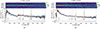 |
Fig. 8. Observational evidence for bursty SFHs in JADES/HST-DEEP. Left: Example of a galaxy in a lull phase at redshift z = 4.5. The spectrum is blue with a quite steep UV slope, but low EW in Hα, and [OIII], and it exhibits a quite strong Balmer break. Right: Example of a galaxy in a regular phase at redshift z = 4.9. The spectrum is blue with a steep UV slope, but quite low EW in Hα, Hβ, and [OIII], and it exhibits a marginal Balmer break. Both galaxies exhibit low EW in the nebular emission lines. |
4.2. Burstiness as a function of redshift z and M⋆
Fig. 9 shows the (SFRneb, 10) mass planes color-coded by the ratio SFRcont, 10/SFRcont, 90, that is, the ratio of the SFR averaged over the last 10 Myr and the SFR averaged between 10 to 100 Myr. The data were divided into the three redshift bins, as indicated. SFRcont, 10 and SFRcont, 90 were inferred with a stellar population fitting with PPXF. We used SFRcont, 90 because it is estimated from a distinct set of weights in the SSP grid, that is, we avoided a correlation by construction.
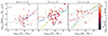 |
Fig. 9. Observational evidence for bursty SFHs: SFR mass plane color-coded by the ratio of the SFR over the last 10 Myr (SFRcont, 10), and 10–100 Myr (SFRcont, 90) before the epoch of observation. Both tracers are inferred from nonparametric SSP fitting of the stellar continuum with PPXF. Each data point represents a single galaxy. The galaxies for which no SFR could be measured are plotted with upper limits. Some are below the quenching threshold and clearly quiescent, while some residual star formation cannot be ruled out for others. More details are given in Fig. 2. In agreement with the theoretical predictions from Ma et al. (2018), Yung et al. (2019), a large fraction of our sample is star bursting, particularly at high redshift and at low mass. In contrast, many galaxies with SFRcont, 10/SFRcont, 90 ≈ 1 lie on the MS predicted by these simulations. |
The ratio of the two PPXF SFR tracers over different timescales indicates whether a single galaxy is in a burst, a regular, or a lull phase at the epoch of observation. The study of the variation in this ratio of galaxies with otherwise similar properties provides important evidence for the burstiness of this galaxy population.
A complementary perspective and important validation of our observational evidence for the variation of star formation burstiness with redshift z and M⋆ is presented in Fig. 10. We investigated burstiness based on the ratio of SFRneb, 10 and SFRcont, 100 (see left plot). The plot on the right shows SFRcont, 10/SFRcont, 90, as in Fig. 9. These results are consistent with the results presented above: The low-mass and high-redshift galaxy populations are clearly burstier, and the high-mass and low-redshift populations exhibit more galaxies in regular phases. As described above, in the low-mass and high-redshift populations, we predominantly observe galaxies in a burst phase, which is likely an observation bias (Sun et al. 2023). Crucially, the two plots show strong evidence for bursty SFHs based on two different methods. The left panel shows that SFRneb, 10/SFRcont, 100 traces burstiness using independent information from the nebular Balmer lines and the stellar continuum (similar to directly estimating the average SFR over timescales of 100 Myr from the UV-luminosity), and the right panel shows SFRcont, 10/SFRcont, 90, which self-consistently traces bursty SFHs from the information about the stellar continuum alone. However, in order to confirm the bursty SFH scenario, galaxies in mini-quenched phases have to be observed. Observational evidence and a discussion of this is presented in the next subsection.
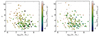 |
Fig. 10. Stellar mass and redshift dependence of the burstiness in galaxy SFHs as inferred from the JADES/HST-DEEP sample. Left: Average star formation over the last ∼10 Myr (color-coded), as traced by Balmer emission lines, relative to the average SFR over the last 100 Myr, as traced by the stellar populations. Right: Relative SFRs inferred from the stellar populations, averaged over the last 10 Myr, and 10–100 Myr before the epoch of observation (indicated as SFRcont, 10 and SFRcont, 90, respectively). The green galaxies are in a regular state at the epoch of observation, white/light galaxies are in a burst, dark galaxies are in a lull, and black galaxies are (mini-)quenched or permanently quenched. |
4.3. Discovery of another (mini-)quenched galaxy at high redshift
In Fig. 11 we present another high-redshift non- or only weakly star-forming galaxy5, with a clearly determined redshift of z = 4.4, which is in addition to the post-starburst galaxy presented in Strait et al. (2023) and the fully (mini-)quenched galaxy JADES-GS-z7-01-QU in Looser et al. (2024a). As in the spectra of these two, we observe a clear Lyα drop and a weak Balmer break. The stellar continuum of the spectrum is similar to the Strait et al. (2023) object at z = 5.2 at a slightly lower redshift and with a stellar mass of M⋆ = 107.8 M⊙. However, as in JADES-GS-z7-01-QU, there is no evidence for ongoing star formation on timescales of 10 Myr as traced by the nebular Balmer emission lines. The stellar mass inferred for JADES-GS-z7-01-QU by our PPXF method is M⋆ = 108.2 M⊙, which is ∼0.5 dex lower than the masses inferred by the other three codes in Looser et al. (2024a).
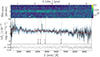 |
Fig. 11. More spectroscopic evidence for (mini-)quenching at high redshift: The Lyα drop and the Balmer break of JADES-GS+53.16136-27.77803 clearly establish the redshift at z = 4.4. The absence of emission lines suggests that this galaxy is in a quiescent phase (which is likely only temporarily) and has not formed a significant amount of stellar mass over the last 10 Myr before the epoch of observation. |
The finding of this additional (mini-)quenched galaxy supports the scenario in which extreme burstiness can even lead to a complete suppression of star formation, at least for short periods of a few 10 Myr.
5. Discussion
5.1. Short-timescale SFR from the stellar continuum
Our approach to measuring SFHs based on PPXF is substantially different from Bayesian inference methods (to name only a few, BEAGLE, Chevallard & Charlot 2016; PROSPECTOR, Johnson et al. 2021, BAGPIPES, Carnall et al. 2018; FADO, Gomes & Papaderos 2017; CIGALE, Noll et al. 2009; and PROSPECT, Robotham et al. 2020). To some extent, all these codes aim to reduce the number of degrees of freedom that determine a galaxy SED by adopting various physically motivated parameterizations and priors. All these assumptions affect the recovered galaxy parameters (e.g., Carnall et al. 2019b; Leja et al. 2019; Sandles et al. 2022).
Another critical difference between the Bayesian approach and our method is that they include a nebular continuum (which can be substantial in extremely young stellar populations, e.g. Byler et al. 2017; Pappalardo et al. 2021) and differential dust attenuation (Charlot & Fall 2000).
However, our approach also presents advantages, and has been demonstrated to work both in the local Universe (e.g., Lu et al. 2023; Zhu et al. 2024, 2023; Barone et al. 2018, 2022) and at redshifts z ≈ 1 (Cappellari 2023). In particular, we have recently shown that PPXF without the use of any priors infers a realistic chemical evolution history for local quiescent and star-forming galaxies (Looser et al. 2024b).
In addition, and central to this work, we showed in Fig. 7 that SFRcont, 10 agrees excellently with SFRneb, 10, even though these two measurements were obtained completely independently. By definition, SFRcont, 10 probes the last 10 Myr of the SFH, as inferred by fitting the stellar continuum. SFRneb, 10, on the other hand, is based on Hα, which is itself an indirect measure of the ionizing continuum. Because this continuum comes from massive stars with lifetimes shorter than 10 Myr, SFRneb, 10 probes timescales of 3–10 Myr, comparable to SFRcont, 10 (e.g., Kennicutt 1998). The good agreement between these two observables is therefore expected. However, while SFRcont, 10 is inferred primarily through the UV continuum redward of Lyα, SFRneb, 10 measures the (highly absorbed) UV continuum blueward of Lyα. In principle, the correct SFR could arise for the wrong reason, for example, our model neglects both the strong nebular continuum and its suppression due to differential dust attenuation. Although we cannot rule out this hypothesis, it seems unlikely that the agreement between SFRcont, 10 and SFRneb, 10 arises from two large systematic errors that cancel each other out.
In the right panel of Fig. 7, we present a comparison between SFRneb, 10 and SFRcont, 100, that is, the average SFR over 100 Myr before the epoch of observation, as inferred from the stellar continuum. This traces the average star formation activity over the same timescales as empirical tracers based on rest-frame UV emission (e.g. Shivaei et al. 2015). The correlation is again strong, but the scatter is much larger than between SFRneb, 10 and SFRcont, 10. This is well known and is commonly interpreted as a measure of the star formation burstiness (e.g., Weisz et al. 2012).
We note that our SFR indicator may be useful for an independent exploration of galaxy escape fractions fesc. Certain empirical estimators of fesc compare a pair of observables, the equivalent width of recombination lines (e.g., EW(Hβ) or EW(Lyα)) and the UV slope β to a grid of models (e.g. Zackrisson et al. 2013; Topping et al. 2022; Flury et al. 2022; Saxena et al. 2024). Our method combines the full shape of the UV and visible continuum to infer amount of stellar mass of various ages. In principle, galaxies with high fesc should manifest as outliers in the SFRneb, 10–SFRcont, 10 correlation, with the latter higher proportionally to fesc.
5.2. Stellar population age and dust attenuation trends
The trends of stellar age as a function of M⋆, ΔMS and z presented in Fig. 2 provide a first measure of the burstiness. The mass-weighted stellar age averages the ages of the stars that formed over a long time-span from the formation of the galaxy to the epoch of observation, while SFRneb, 10 only traces the most recent stars that formed (over timescales of 3–10 Myr). If galaxies evolved steadily, we would expect a perfect correlation between ΔMS and age. In contrast, a rapidly varying (burstier) SFH would lead to an inconsistent relation between SFRneb, 10 and the mass-weighted age; for example, galaxies that have stopped forming stars rapidly will have low current SFRneb, 10 (thus lying below the MS), but young ages (10–30 Myr), which increases the scatter between ΔMS and age itself for the population as a whole. This seems exactly what we observe in Fig. 2; while most young galaxies (age ≈ 10–30 Myr) are on and above the MS, there are several examples of equally young systems below the MS.
Even though the locus of the star-forming MS is likely affected by sample bias, we detect large scatter in the SFR of the youngest galaxies, larger than the typical observational uncertainties on SFR itself. However, for the precision of the age measurements, our data may be dominated by systematic uncertainties. A comparison with different measurements, for example, from Bayesian SED modeling, may help us to quantify which fraction of the observed scatter about the age–ΔMS relation is intrinsic and which is due to measurement uncertainties.
Nonetheless, despite this scatter, the overall trends of decreasing age with decreasing M⋆ and with increasing z and SFR are clear, which is a reassuring independent test of the quality of our measurements. In particular, the trend of decreasing age with increasing z is not simply due to our truncation of the age grid to match the age of the Universe at the redshift of each galaxy simply because in each redshift bin, we see systematic age differences across the SFR–M⋆ plane. In addition, this trend does not arise from observational bias either: If there were significant numbers of young galaxies below the MS, they would be systematically brighter than older galaxies at the same location on the SFR–M⋆ plane.
The trends between age and M⋆ and SFR have also been observed in the local Universe (z < 0.1; e.g., Looser et al., in prep.), where they are interpreted as a manifestation of SFHs that self-correlate over the MS timescale 1/sSFR (Tacchella et al. 2020; Looser et al. 2024b). While this timescale is about a few billion years in the local Universe, at high redshift, 1/sSFR is likely much shorter, of about 100 Myr or even shorter, so the age correlations we observe do not rule out bursty SFHs ipso facto.
The overall picture of younger galaxies above the MS at higher z and lower M⋆ agrees with the results we obtained from stacks of individual SFHs in z–M⋆–ΔMS bins (Figs. 3–5). Additionally, the stacked SFHs appear to show that massive galaxies formed generally earlier and that their SFR are stationary or declining on average.
Similarly to what we found for stellar age, dust reddening also trends with M⋆, ΔMS and z (Fig. 6). These trends are as arguably expected: Quiescent galaxies and galaxies below the MS show little or no evidence for dust, whereas star-bursting galaxies exhibit significant reddening. Furthermore, nearly all galaxies at low redshift experience some dust attenuation of the stellar continuum, while we do not observe any highly obscured objects at high z (this is probably not due to an observability bias, but might be due to sample selection bias, i.e., with which targets the JADES/HST-DEEP MSA was populated as part of target allocation strategy; see Sandles et al. (2024).
Massive galaxies tend to be dustier than low-mass galaxies on average. These trends are derived purely from the stellar continuum, but they agree excellently with what we infer from nebular recombination lines (Sandles et al. 2024); this is another independent confirmation of our approach. When we assume that dust attenuation roughly traces the amount of cold gas, these trends suggest that SFR and ΔMS are tightly coupled with the availability of fuel. For galaxies in the mass range we explored, this conclusion agrees excellently with the prediction of some simulations, which argued that the instantaneous ΔMS of a galaxy is driven by rapid gas accretion and depletion. This is due to the subordinate role of the dampening effect afforded by large disk reservoirs, which is important in higher-mass galaxies and at lower redshifts (Wang et al. 2019).
5.3. Bursty SFHs
Theoretical models agree that the scatter about the star-forming main sequence increases with increasing z because the conditions of the primordial universe are conducive to stronger feedback, which results in galaxies with more bursty star-formation histories (Ceverino et al. 2018; Lovell et al. 2023; Ma et al. 2018; Faucher-Giguère 2018; Tacchella et al. 2020). However, these models differ in how star formation and feedback are implemented, and therefore, they provide different quantitative predictions. A comparison with observations is particularly useful because burstiness is predicted in models both with and without AGN feedback, which is thought to also affect the evolution of low-mass galaxies (Koudmani et al. 2019).
Several studies have found prescriptions of how to measure burstiness (e.g., the power spectral density approach of Caplar & Tacchella 2019) and/or how to infer burstiness from observational data (Weisz et al. 2012; Faisst et al. 2019; Wang et al. 2016; Caplar & Tacchella 2019; Speagle et al. 2014).
However, the observational confirmation and characterization of bursty SFHs is still challenging. The key problem is that burstiness manifests itself as scatter about the MS and between SFR indicators averaged over different timescales. The difficulty is then to extricate the information-laden scatter rooted in physical burstiness from the incidental contribution of measurement noise.
We argue that we overcame this difficulty in two ways. By using a nonparametric approach, we avoided biasing our solutions toward particular SFH shapes. In practice, adding a regularization is similar to introducing a prior, with higher regularization biasing the solution toward less bursty SFHs. This is precisely why we apply regularization: to determine whether the data favors bursty SFHs, despite the priors pushing against it.
Our nonparametric approach allows for greater flexibility in the shape of SFHs but naturally comes at the cost of reduced precision. JADES provides us with the means to overpower low-precision measurements; its exceptionally deep spectroscopy spans the rest-frame UV and rest-frame optical, that is, the regions of the spectrum that are dominated by stellar emission, in particular, stars with ages younger than 100 Myr. We used two alternative measures of burstiness, that is, SFRneb, 10/SFRcont, 100 (Fig. 10, left), and SFRcont, 10/SFRcont, 90 (Figs. 9 and 10, right)6. These are still empirical estimators that may be difficult to compare directly to theoretical predictions. However, compared to the classic burstiness measure SFRneb, 10/SFRuv, 100, we improved the method by using the entire information encoded in the spectrum, while SFRUV, 100 reduces the SFH in the last 100 Myr to a single degenerate observable, that is, the UV luminosity.
In the future, it will be crucial to compare our results with Bayesian stellar population modeling codes, which might provide a more physically motivated reconstruction of the star formation history by incorporating complex burst patterns driven by physical expectations. In particular, Bayesian approaches could combine the posterior probability distributions for large samples of galaxies to constrain population-wide parameters such as the burstiness (e.g., using the hierarchical approach of Wan et al., in prep.).
In Section 4, we presented observational evidence for bursty SFHs in high-redshift and in low-mass systems based on full spectral fitting with PPXF (Figs. 9 and 10). Qualitatively, this agrees with model expectations. As we mentioned, at fixed stellar mass, galaxies at higher redshift had burstier histories. Conversely, at fixed redshift, the burstiness increases with decreasing stellar mass. The physical reason for this burstiness might be different: In high-z galaxies, burstiness is likely a result of an abundant amount of cold dense gas and high stochasticity of the gas inflow rate combined with powerful supernovae and AGN feedback, while in low-mass galaxies, local starbursts in short-lived giant molecular clouds might cause the burstiness on short timescales (Tacchella et al. 2020).
We observed interesting trends with redshift z, ΔMS, and M⋆: (a) We preferentially observed bursting systems (indicated by light colors in Fig. 9) at higher redshift and in low-mass systems, as is arguably expected from observation bias (Sun et al. 2023). (b) These systems are preferentially situated above the MS, as traced by the nebular emission lines, in agreement with the interpretation that they are in a burst phase. (c) Galaxies on the MS are often in a regular phase. (d) Galaxies below the MS are often in lull phases, but also in regular phases, which might indicate reduced star formation activity over extended timescales. (e) High-mass systems are often found in regular phases, particularly in the first two redshift bins. This suggests a more regular evolution of these systems and is again consistent with theoretical expectations (e.g., Ceverino et al. 2018).
We emphasize that the analysis presented here is a high-redshift view on SFHs. In the local Universe, the SFHs of galaxies are different. Studies of large galaxy samples at redshift z = 0 (e.g., MaNGA; Bundy et al. 2015 or SDSS; Abdurro’uf et al. 2022) show a strong connection between the star formation activity of a galaxy at the epoch of observation and its past SFH. SFHs of galaxies are steadier, and their evolution is dominated by different physical processes. For example, galaxies dominantly quench through starvation (Peng et al. 2015; Trussler et al. 2020, 2021; Looser et al. 2024b), and the environment (Peng et al. 2010) or outflows play a secondary effect. Conversely, our analysis presented here strongly suggests that SFHs in the young Universe are bursty.
The critical question remains whether the high SFRcont, 10/SFRcont, 90 we measure reflects just the tail of a much less bursty and much larger galaxy population. Intriguingly, the complementary approach based on photometry alone seems to reach similar conclusions (Endsley et al. 2023, 2024). These authors used SED modeling with BEAGLE of deep nine-band NIRCam imaging from JADES, which revealed evidence for lulling galaxy candidates.
However, to unambiguously prove the bursty SFH interpretation, galaxies in lull phases and (mini-)quenched galaxies have to be confirmed spectroscopically. We discuss this next.
5.4. Galaxies in lulls and (mini-)quenching at high redshift
In Section 4.1 we showed that the extraordinary depth and data quality of JADES are capable of probing well below the starburst regime. We showed examples of both galaxies on the MS (i.e., in regular phases; Fig. 8, right) and below the MS (in lull phases; Fig. 8, left). We further showed that JADES is capable of probing galaxies that are formally below the redshift-dependent quiescent threshold in all three redshift bins (Fig. 2). These galaxies show no evidence for emission lines (Fig. 11 and Looser et al. 2024a), and they experience (potentially short-lived) phases of quiescence. The fact that these galaxies are present in our sample argues against our findings that burstiness is a result of limited sensitivity. However, the fraction of lull or (mini-)quenched galaxies is clearly lower than that of starburst systems (Fig. 2). This could ostensibly be the undesired outcome of the initial sample selection, which prioritized objects with high-confidence photometric redshifts. In practice, these are galaxies with stronger broadband drops that are due in turn to either a Lyman continuum drop or to high-equivalent-width nebular emission, both of which are generally associated with a high SFR (Bunker et al. 2024). The difficulty of an unbiased sample selection is highlighted by the complementary approach based on JADES photometry (Endsley et al. 2023), which reported very similar results (i.e., an overabundance of starburst galaxies) based on a NIRCam-selected sample. For our spectroscopic sample, the fact that the only mini-quenched galaxy at z > 5 is relatively massive and young (M⋆ = 5 × 10⁸ M⊙, 108 yr; Looser et al. 2024a) suggests that in this redshift range, we are limited by the depth of JADES. This is again supported by the fact that in the intermediate-redshift bin, we are able to confirm a mini-quenched galaxy with M⋆ = 8 × 10⁷ M⊙ and age 107.9 yr, which clearly is in the low-mass regime where strong feedback is expected to trigger short-lived mini-quenching (Ceverino et al. 2018; Ma et al. 2018; Dome et al. 2024).
According to the models, the burstiness of the star formation should only increase probing masses M⋆ ≈ 106 M⊙. The galaxies we present here, together with those presented in recent works (Strait et al. 2023; Looser et al. 2024a), showed that we finally begin to probe the obverse face of the burstiness phenomenon. However, a more quantitative understanding will probably require the expensive combination of larger samples and/or even deeper observations. In particular, separating the degenerate effects of mass and redshift will only be feasible with thousands of objects that effectively probe the parameter space.
Nonetheless, the analysis presented in this work is strong evidence that galaxies at high redshift are bursty and go through these lulling and (mini-)quenched phases. In the next section, we discuss the effects of the observation bias in more detail.
6. Summary and conclusions
We combined the nonparametric approach of the PPXF software with the marvelous depth of JWST/NIRSpec MSA spectroscopy to offer a view of the star formation histories (SFHs) of low- to intermediate-mass galaxies (106 < M⋆ < 109.5 M⊙) up to cosmic dawn, between redshifts 0.6 ≲ z ≲ 11.
The key results of this paper are listed below.
-
The correlation of the mass-weighted stellar age with M⋆, z, and SFR already existed well before the local Universe and even earlier than cosmic noon, at redshifts as high as 5 < z < 11 (Fig. 2). All else being equal, age increases with increasing M⋆ and decreases with increasing z and with increasing distance from the star-forming main sequence, ΔMS. We found consistent trends in the stellar populations in stacks of SFHs in z–M⋆–ΔMS bins. These correlations probably do not result from sample or observation bias, and they argue that the SFHs of galaxies are correlated on timescales comparable to the main-sequence timescale of 1/sSFR (where sSFR is the specific star-formation rate).
-
However, the trends between age, M*, and SFR have a large scatter, with examples of young stellar populations also below the main sequence. This is a first indication of bursty star formation.
-
We introduced and validated a short-timescale continuum-based SFR indicator, averaged over the last 10 Myr before the epoch of observation (SFRcont, 10). Our analysis shows strong agreement between SFRcont, 10 and the well-established SFR tracer based on Balmer-series nebular emission lines (SFRneb, 10). We compared SFRcont, 10 to the average over the last 10–100 Myr (SFRcont, 90) as an estimate of the SFH burstiness.
-
By using these parameters, we presented additional observational evidence that the SFHs of high-redshift and low-mass galaxies are bursty. Specifically, we used SFRcont, 10/SFRcont, 90 to investigate the burstiness in the SFR-mass plane and as a function of redshift, and we found that high-redshift and low-mass galaxies have particularly bursty SFHs, while more massive and lower-redshift systems evolve more steadily.
-
We reported the discovery of another low-mass galaxy in the (mini-)quenched phase, at redshift z = 4.4. This galaxy lies well within the mass regime in which numerical simulations predict that star formation is dominated by short and intense bursts. Therefore, the quiescence of this galaxy might only be transient, as discussed in Looser et al. (2024a).
-
We argued that we see most targets at the observability frontier, that is, at the highest redshifts and at the lowest masses, preferentially in star-bursting phases. Their more regular, lulling and (mini-)quenched counterparts are likely at the bottom edge of the observability window at the epoch of observation, even for the JWST.
-
Finally, we used the stellar E(B − V) as a proxy for the amount of dust and found that E(B − V) increases with increasing M⋆ and ΔMS, possibly as a result of the correlation between the dust and gas mass and between the gas mass and SFR in step. We found that E(B − V) decreases at the highest redshifts, although most galaxies at z > 5 still have some dust.
However, this is only the beginning of the investigation of stellar populations and bursty SFHs and (mini-)quenching at high redshift with galaxy population samples observed with the JWST: Larger statistical samples of high-S/N galaxy spectra will enable the investigation and quantification of selection effects, which are key to this type of analysis, and the quantification of various physical aspects of stellar populations and bursty SFHs, such as the duty cycles, oscillation times, and the short- and long-term variability, for example, in the framework of the power spectral density (PSD; Tacchella et al. 2020). A detailed comparison to numerical cosmological simulations will be crucial for analyzing the complex interplay of the physical mechanisms that contribute to making SFHs bursty. Upcoming observations with the JWST will provide such a sample and will continue to reveal the physics processes that shape the observed differing assembly histories of galaxies in the early Universe.
Where MS describes the positive scaling relation between M⋆ and SFR of the star-forming galaxy population (e.g. Sandles et al. 2022).
For a sub-sample of targets, also higher-resolution grating spectra were obtained as a part of this program. However, in this work, we focus on the PRISM spectra, which are more relevant for the stellar continuum.
https://pypi.org/project/ppxf/; version 8.1.0
These SSP templates are available from the author C. Conroy upon reasonable request.
For the public JADES NIRCam imaging of the target (ID:10009848, coordinates: RA = 53.16136 and Dec = –27.77803) please see: https://jades.idies.jhu.edu/public/?ra=53.1614880dec=-27.7779085zoom=10
We note that the inferred burstiness does not depend on the χ2-value of the fit.
Acknowledgments
TJL, FDE, RM, LS, WB, LS, JS and JW acknowledge support by the Science and Technology Facilities Council (STFC), by the ERC through Advanced Grant 695671 “QUENCH”, and by the UKRI Frontier Research grant RISEandFALL. TJL and ALD acknowledge support by the STFC Center for Doctoral Training in Data Intensive Science. RM also acknowledges funding from a research professorship from the Royal Society. ECL acknowledges support of an STFC Webb Fellowship (ST/W001438/1). SA and BRP acknowledge support from Grant PID2021-127718NB-I00 funded by the Spanish Ministry of Science and Innovation/State Agency of Research (MICIN/AEI/10.13039/501100011033). SC acknowledges support by European Union’s HE ERC Starting Grant No. 101040227 – WINGS. AJB, and JC acknowledge funding from the “FirstGalaxies” Advanced Grant from the European Research Council (ERC) under the European Union’s Horizon 2020 research and innovation program (Grant agreement No. 789056). HÜ gratefully acknowledges support by the Isaac Newton Trust and by the Kavli Foundation through a Newton-Kavli Junior Fellowship. JW further acknowledges support from the Fondation MERAC. KB acknowledges support by the Australian Research Council Centre of Excellence for All Sky Astrophysics in 3 Dimensions (ASTRO 3D), through project number CE170100013. The Cosmic Dawn Center (DAWN) is funded by the Danish National Research Foundation under grant no.140. DJE is supported as a Simons Investigator. ALD thanks the Cambridge Harding postgraduate program. DJE BDJ and BER acknowledge support by the JWST/NIRCam contract to the University of Arizona, NAS5-02015. RS acknowledges support from a STFC Ernest Rutherford Fellowship (ST/S004831/1). The research of CCW is supported by NOIRLab, which is managed by the Association of Universities for Research in Astronomy (AURA) under a cooperative agreement with the National Science Foundation.
References
- Abdurro’uf, Accetta, K., Aerts, C., et al. 2022, ApJS, 259, 35 [NASA ADS] [CrossRef] [Google Scholar]
- Barone, T. M., D’Eugenio, F., Colless, M., et al. 2018, ApJ, 856, 64 [Google Scholar]
- Barone, T. M., D’Eugenio, F., Scott, N., et al. 2022, MNRAS, 512, 3828 [NASA ADS] [CrossRef] [Google Scholar]
- Bisigello, L., Caputi, K. I., Grogin, N., & Koekemoer, A. 2018, A&A, 609, A82 [NASA ADS] [CrossRef] [EDP Sciences] [Google Scholar]
- Bruzual, G., & Charlot, S. 2003, MNRAS, 344, 1000 [NASA ADS] [CrossRef] [Google Scholar]
- Bundy, K., Bershady, M. A., Law, D. R., et al. 2015, APJ, 798, 7 [Google Scholar]
- Bunker, A. J., Cameron, A. J., Curtis-Lake, E., et al. 2024, A&A, 690, A288 [NASA ADS] [CrossRef] [EDP Sciences] [Google Scholar]
- Byler, N., Dalcanton, J. J., Conroy, C., & Johnson, B. D. 2017, ApJ, 840, 44 [Google Scholar]
- Calzetti, D., Kinney, A. L., & Storchi-Bergmann, T. 1994, ApJ, 429, 582 [Google Scholar]
- Calzetti, D., Armus, L., Bohlin, R. C., et al. 2000, APJ, 533, 682 [Google Scholar]
- Caplar, N., & Tacchella, S. 2019, MNRAS, 487, 3845 [NASA ADS] [CrossRef] [Google Scholar]
- Cappellari, M. 2017, MNRAS, 466, 798 [Google Scholar]
- Cappellari, M. 2023, MNRAS, 526, 3273 [NASA ADS] [CrossRef] [Google Scholar]
- Caputi, K. I., Lagache, G., Yan, L., et al. 2007, ApJ, 660, 97 [NASA ADS] [CrossRef] [Google Scholar]
- Carnall, A. C., McLure, R. J., Dunlop, J. S., & Davé, R. 2018, MNRAS, 480, 4379 [Google Scholar]
- Carnall, A. C., McLure, R. J., Dunlop, J. S., et al. 2019a, MNRAS, 490, 417 [Google Scholar]
- Carnall, A. C., Leja, J., Johnson, B. D., et al. 2019b, ApJ, 873, 44 [Google Scholar]
- Carnall, A. C., McLeod, D. J., McLure, R. J., et al. 2023, MNRAS, 520, 3974 [NASA ADS] [CrossRef] [Google Scholar]
- Ceverino, D., Klessen, R. S., & Glover, S. C. O. 2018, MNRAS, 480, 4842 [NASA ADS] [Google Scholar]
- Ceverino, D., Hirschmann, M., Klessen, R. S., et al. 2021, MNRAS, 504, 4472 [NASA ADS] [CrossRef] [Google Scholar]
- Chabrier, G. 2003, PASP, 115, 763 [Google Scholar]
- Charlot, S., & Fall, S. M. 2000, ApJ, 539, 718 [Google Scholar]
- Chevallard, J., & Charlot, S. 2016, MNRAS, 462, 1415 [NASA ADS] [CrossRef] [Google Scholar]
- Choi, J., Dotter, A., Conroy, C., et al. 2016, ApJ, 823, 102 [Google Scholar]
- Conroy, C., Naidu, R. P., Zaritsky, D., et al. 2019, ApJ, 887, 237 [NASA ADS] [CrossRef] [Google Scholar]
- Curti, M., Maiolino, R., Curtis-Lake, E., et al. 2024, A&A, 684, A75 [NASA ADS] [CrossRef] [EDP Sciences] [Google Scholar]
- Díaz-Santos, T., Armus, L., Charmandaris, V., et al. 2017, ApJ, 846, 32 [Google Scholar]
- Dome, T., Tacchella, S., Fialkov, A., et al. 2024, MNRAS, 527, 2139 [Google Scholar]
- Dressler, A., Vulcani, B., Treu, T., et al. 2023, ApJ, 947, L27 [NASA ADS] [CrossRef] [Google Scholar]
- Dressler, A., Rieke, M., Eisenstein, D., et al. 2024, ApJ, 964, 150 [NASA ADS] [CrossRef] [Google Scholar]
- Eisenstein, D. J., Willott, C., Alberts, S., et al. 2023, ApJ, submitted [arXiv:2306.02465] [Google Scholar]
- Endsley, R., Stark, D. P., Chevallard, J., & Charlot, S. 2021, MNRAS, 500, 5229 [Google Scholar]
- Endsley, R., Stark, D. P., Whitler, L., et al. 2023, MNRAS, 524, 2312 [NASA ADS] [CrossRef] [Google Scholar]
- Endsley, R., Stark, D. P., Whitler, L., et al. 2024, MNRAS, 533, 1111 [NASA ADS] [CrossRef] [Google Scholar]
- Faisst, A. L., Capak, P. L., Emami, N., Tacchella, S., & Larson, K. L. 2019, ApJ, 884, 133 [NASA ADS] [CrossRef] [Google Scholar]
- Faucher-Giguère, C.-A. 2018, MNRAS, 473, 3717 [Google Scholar]
- Ferruit, P., Jakobsen, P., Giardino, G., et al. 2022, A&A, 661, A81 [NASA ADS] [CrossRef] [EDP Sciences] [Google Scholar]
- Flury, S. R., Jaskot, A. E., Ferguson, H. C., et al. 2022, ApJS, 260, 1 [NASA ADS] [CrossRef] [Google Scholar]
- Gallazzi, A., Bell, E. F., Zibetti, S., Brinchmann, J., & Kelson, D. D. 2014, ApJ, 788, 72 [Google Scholar]
- Gardner, J. P., Mather, J. C., Clampin, M., et al. 2006, Space Sci. Rev., 123, 485 [Google Scholar]
- Gardner, J. P., Mather, J. C., Abbott, R., et al. 2023, PASP, 135, 068001 [NASA ADS] [CrossRef] [Google Scholar]
- Gelli, V., Salvadori, S., Ferrara, A., Pallottini, A., & Carniani, S. 2023, ApJ, 954, L11 [NASA ADS] [CrossRef] [Google Scholar]
- Giavalisco, M., Ferguson, H. C., Koekemoer, A. M., et al. 2004, ApJ, 600, L93 [NASA ADS] [CrossRef] [Google Scholar]
- Glazebrook, K., Blake, C., Economou, F., Lilly, S., & Colless, M. 1999, MNRAS, 306, 843 [NASA ADS] [CrossRef] [Google Scholar]
- Gomes, J. M., & Papaderos, P. 2017, A&A, 603, A63 [NASA ADS] [CrossRef] [EDP Sciences] [Google Scholar]
- Gordon, K. D., Clayton, G. C., Misselt, K. A., Landolt, A. U., & Wolff, M. J. 2003, ApJ, 594, 279 [NASA ADS] [CrossRef] [Google Scholar]
- Jakobsen, P., Ferruit, P., Alves de Oliveira, C., et al. 2022, A&A, 661, A80 [NASA ADS] [CrossRef] [EDP Sciences] [Google Scholar]
- Ji, Z., & Giavalisco, M. 2022, ApJ, 935, 120 [NASA ADS] [CrossRef] [Google Scholar]
- Ji, Z., & Giavalisco, M. 2023, ApJ, 943, 54 [NASA ADS] [CrossRef] [Google Scholar]
- Johnson, B. D., Leja, J., Conroy, C., & Speagle, J. S. 2021, ApJS, 254, 22 [NASA ADS] [CrossRef] [Google Scholar]
- Kawata, D., & Gibson, B. K. 2003, MNRAS, 346, 135 [NASA ADS] [Google Scholar]
- Kennicutt, R. C., Jr. 1998, ApJ, 498, 541 [Google Scholar]
- Kennicutt, R. C., & Evans, N. J. 2012, ARA&A, 50, 531 [NASA ADS] [CrossRef] [Google Scholar]
- Koudmani, S., Sijacki, D., Bourne, M. A., & Smith, M. C. 2019, MNRAS, 484, 2047 [NASA ADS] [CrossRef] [Google Scholar]
- Laporte, N., Ellis, R. S., Witten, C. E. C., & Roberts-Borsani, G. 2023, MNRAS, 523, 3018 [NASA ADS] [CrossRef] [Google Scholar]
- Leja, J., Carnall, A. C., Johnson, B. D., Conroy, C., & Speagle, J. S. 2019, ApJ, 876, 3 [Google Scholar]
- Looser, T. J., D’Eugenio, F., Maiolino, R., et al. 2024a, Nature, 629, 53 [Google Scholar]
- Looser, T. J., D’Eugenio, F., Piotrowska, J. M., et al. 2024b, MNRAS, 532, 2832 [NASA ADS] [CrossRef] [Google Scholar]
- Lovell, C. C., Roper, W., Vijayan, A. P., et al. 2023, MNRAS, 525, 5520 [NASA ADS] [Google Scholar]
- Lu, S., Zhu, K., Cappellari, M., et al. 2023, MNRAS, 526, 1022 [NASA ADS] [CrossRef] [Google Scholar]
- Ma, X., Hopkins, P. F., Garrison-Kimmel, S., et al. 2018, MNRAS, 478, 1694 [NASA ADS] [CrossRef] [Google Scholar]
- Maheson, G., Maiolino, R., Curti, M., et al. 2024, MNRAS, 527, 8213 [Google Scholar]
- McDermid, R. M., Alatalo, K., Blitz, L., et al. 2015, MNRAS, 448, 3484 [Google Scholar]
- McLure, R. J., Dunlop, J. S., Cullen, F., et al. 2018, MNRAS, 476, 3991 [Google Scholar]
- Noll, S., Burgarella, D., Giovannoli, E., et al. 2009, A&A, 507, 1793 [NASA ADS] [CrossRef] [EDP Sciences] [Google Scholar]
- Pacifici, C., Kassin, S. A., Weiner, B. J., et al. 2016, ApJ, 832, 79 [Google Scholar]
- Pannella, M., Carilli, C. L., Daddi, E., et al. 2009, ApJ, 698, L116 [Google Scholar]
- Pappalardo, C., Cardoso, L. S. M., Michel Gomes, J., et al. 2021, A&A, 651, A99 [NASA ADS] [CrossRef] [EDP Sciences] [Google Scholar]
- Peng, Y.-J., Lilly, S. J., Kovač, K., et al. 2010, ApJ, 721, 193 [Google Scholar]
- Peng, Y., Maiolino, R., & Cochrane, R. 2015, Nature, 521, 192 [Google Scholar]
- Popesso, P., Concas, A., Cresci, G., et al. 2023, MNRAS, 519, 1526 [Google Scholar]
- Rieke, M. J., Kelly, D. M., Misselt, K., et al. 2023, PASP, 135, 028001 [CrossRef] [Google Scholar]
- Rinaldi, P., Caputi, K. I., van Mierlo, S. E., et al. 2022, ApJ, 930, 128 [NASA ADS] [CrossRef] [Google Scholar]
- Robotham, A. S. G., Bellstedt, S., Lagos, C. d. P., et al. 2020, MNRAS, 495, 905 [NASA ADS] [CrossRef] [Google Scholar]
- Sandles, L., Curtis-Lake, E., Charlot, S., Chevallard, J., & Maiolino, R. 2022, MNRAS, 515, 2951 [NASA ADS] [CrossRef] [Google Scholar]
- Sandles, L., D’Eugenio, F., Maiolino, R., et al. 2024, A&A, 691, A305 [NASA ADS] [CrossRef] [EDP Sciences] [Google Scholar]
- Santini, P., Fontana, A., Castellano, M., et al. 2017, ApJ, 847, 76 [NASA ADS] [CrossRef] [Google Scholar]
- Saxena, A., Bunker, A. J., Jones, G. C., et al. 2024, A&A, 684, A84 [NASA ADS] [CrossRef] [EDP Sciences] [Google Scholar]
- Shapley, A. E., Sanders, R. L., Salim, S., et al. 2022, ApJ, 926, 145 [NASA ADS] [CrossRef] [Google Scholar]
- Shapley, A. E., Sanders, R. L., Reddy, N. A., Topping, M. W., & Brammer, G. B. 2023, ApJ, 954, 157 [NASA ADS] [CrossRef] [Google Scholar]
- Shivaei, I., Reddy, N. A., Steidel, C. C., & Shapley, A. E. 2015, ApJ, 804, 149 [NASA ADS] [CrossRef] [Google Scholar]
- Smit, R., Bouwens, R. J., Labbé, I., et al. 2014, ApJ, 784, 58 [NASA ADS] [CrossRef] [Google Scholar]
- Smit, R., Bouwens, R. J., Franx, M., et al. 2015, ApJ, 801, 122 [Google Scholar]
- Speagle, J. S., Steinhardt, C. L., Capak, P. L., & Silverman, J. D. 2014, ApJS, 214, 15 [Google Scholar]
- Strait, V., Brammer, G., Muzzin, A., et al. 2023, ApJ, 949, L23 [NASA ADS] [CrossRef] [Google Scholar]
- Sun, G., Faucher-Giguère, C.-A., Hayward, C. C., & Shen, X. 2023, MNRAS, 526, 2665 [NASA ADS] [CrossRef] [Google Scholar]
- Tacchella, S., Dekel, A., Carollo, C. M., et al. 2016, MNRAS, 457, 2790 [Google Scholar]
- Tacchella, S., Forbes, J. C., & Caplar, N. 2020, MNRAS, 497, 698 [Google Scholar]
- Tacchella, S., Conroy, C., Faber, S. M., et al. 2022, ApJ, 926, 134 [NASA ADS] [CrossRef] [Google Scholar]
- Topping, M. W., Stark, D. P., Endsley, R., et al. 2022, ApJ, 941, 153 [NASA ADS] [CrossRef] [Google Scholar]
- Trussler, J., Maiolino, R., Maraston, C., et al. 2020, MNRAS, 491, 5406 [Google Scholar]
- Trussler, J., Maiolino, R., Maraston, C., et al. 2021, MNRAS, 500, 4469 [Google Scholar]
- Vidal-García, A., Charlot, S., Bruzual, G., & Hubeny, I. 2017, MNRAS, 470, 3532 [Google Scholar]
- Wang, T., Elbaz, D., Daddi, E., et al. 2016, ApJ, 828, 56 [NASA ADS] [CrossRef] [Google Scholar]
- Wang, E., Lilly, S. J., Pezzulli, G., & Matthee, J. 2019, ApJ, 877, 132 [NASA ADS] [CrossRef] [Google Scholar]
- Weisz, D. R., Johnson, B. D., Johnson, L. C., et al. 2012, ApJ, 744, 44 [NASA ADS] [CrossRef] [Google Scholar]
- Whitaker, K. E., Pope, A., Cybulski, R., et al. 2017, ApJ, 850, 208 [NASA ADS] [CrossRef] [Google Scholar]
- Whitler, L., Endsley, R., Stark, D. P., et al. 2023, MNRAS, 519, 157 [Google Scholar]
- Yung, L. Y. A., Somerville, R. S., Popping, G., et al. 2019, MNRAS, 490, 2855 [NASA ADS] [CrossRef] [Google Scholar]
- Zackrisson, E., Inoue, A. K., & Jensen, H. 2013, ApJ, 777, 39 [NASA ADS] [CrossRef] [Google Scholar]
- Zhu, K., Lu, S., Cappellari, M., et al. 2023, MNRAS, 522, 6326 [NASA ADS] [CrossRef] [Google Scholar]
- Zhu, K., Lu, S., Cappellari, M., et al. 2024, MNRAS, 527, 706 [Google Scholar]
Appendix A: PPXF stellar population grid fitting example
To show an illustrative example of our SFH inference methodology based on PPXF, we show the results of the fitting of the spectrum shown in Fig. 1b. In Fig. A.1 the light-weighted 2D grid of SSP-weights is presented, where the age of the SSP templates is given on the x-axis, and the stellar metallicity on the y-axis, respectively. Fig. A.2 shows the conversion of these weights into a non-parametric mass-weighted SFH.
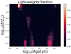 |
Fig. A.1. Example: PPXF stellar population inference from the spectrum presented in Fig. 1b. The fitted light-weighted SSP age-metallicity grid. |
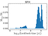 |
Fig. A.2. Example: PPXF SFH inferred from the spectrum presented in Fig. 1b. The 2D weight-grid (shown in Fig.A.1) converted to a mass-weighted SFH, where the ages of the SSP-templates are equivalent to the star formation activity at that look-back time. The SFH is normalized by the total stellar mass of the galaxy M⋆. |
Appendix B: Comparison between PPXF and BEAGLE stellar mass
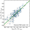 |
Fig. B.1. Comparison between the stellar masses inferred by PPXF and BEAGLE. The orange line indicates the 1:1 line. The green solid line show the best-fit relation between the two mass-estimated. The dashed green lines show the 1-sigma error on the best-fit. The masses show a strong correlation, with an RMS-scatter of 0.2 dex, but an offset of 0.2 dex at the low-mass end. |
In Fig. B.1, we present a comparison between the stellar masses inferred by PPXF, see details in section 2.3, and those inferred by the Bayesian inference code BEAGLE (Chevallard & Charlot 2016). The BEAGLE-derived masses are computed assuming a parametric delayed exponential SFH combined with a 10 Myr burst; and adopting an updated version of the BC03 stellar population model library (Bruzual & Charlot 2003), as described in Vidal-García et al. (2017). More details on the BEAGLE stellar masses for the JADES/HST-DEEP sample are given in Curti et al. (2024) and Chevallard et al. (in prep.). For both the PPXF and the BEAGLE masses we assume a Chabrier IMF.
Overall, we find a strong correlation between the stellar masses inferred by the two codes, with a linear fit of log10(M∗,BEAGLE) = (0.91 ± 0.04) × (log10(M∗,PPXF) − 8.0) +(8.11 ± 0.03) and a RMS-scatter of 0.2 dex. However, we note a 0.2 dex offset in overall normalization at the low-mass end. The larger masses inferred by BEAGLE compared to PPXF likely stem from the different modeling approaches: firstly, the SFHs inferred with PPXF are fitted with a penalty on the number of SSP templates used. In other words, in case of out-shining, PPXF tends to not fit any old stellar populations - which would contribute little light, but strongly increase the stellar mass. Secondly, BEAGLE’s delayed tau SFH model effectively introduces a continuity prior, while PPXF will choose to not fit any (mid-age) SSPs unless the data demands it. This can lead to (possibly physical?) gaps, i.e. quiescent/mini-quenched phases in the PPXF SFHs, see e.g. Fig. A.2.
All Figures
|
Fig. 1. Examples of JADES/HST-DEEP spectra at high redshift. The fitted PPXF continuum is shown in red, and the nebular emission lines are shown in yellow. The bottom panel indicates the reduced residuals of the fits The vertical dashed lines mark the rest-frame wavelengths of strong nebular emission lines. The noise is indicated by the shaded blue regions. The upper panel shows the S/N of the combined 2D spectrum (the 1D spectrum was not extracted from the combined 2D spectrum). Left: A star-bursting galaxy at redshift z = 5.9 that might be rejuvenating. We note the simultaneous presence of (i) a Balmer break and a shallow β-slope, and (ii) strong nebular emission lines. Right: A weakly star-forming galaxy at redshift z = 3.6. We note the simultaneous presence of (i) a strong Balmer break and a shallow β-slope, and (ii) weak nebular emission lines. |
| In the text | |
|
Fig. 2. SFR-mass plane, color-coded by the average mass-weighted stellar ages measured by PPXF in three different redshift bins. Each data point represents a single galaxy. The blue lines represent a simple linear fit to the SFR–M⋆ relation of this sample in that redshift bin. For reference, various observational MS estimates (Santini et al. 2017; Popesso et al. 2023; Rinaldi et al. 2022) and predictions from simulations (Ma et al. 2018; Yung et al. 2019) are presented, as indicated by the labels. We extrapolated these MS by ca. 0.5 dex in stellar mass where necessary to compare them to our lower-mass sample. The three dotted lines indicate the quenched threshold for the same redshifts (see main text). The error bar in the upper left corner represents the RMS errors for M⋆ and SFR for the entire sample. Quiescent and (mini-)quenched galaxies and other galaxies for which no SFR could be estimated because the relevant nebular emission lines were not detected are plotted with upper limits. |
| In the text | |
|
Fig. 3. Mass-weighted stacks of normalized SFHs of galaxies in three bins each of M⋆ and ΔMS in the redshift range 0 < z < 2. The number in the legend of each panel indicates the number of galaxies that contribute to the stack. In each bin, the SSP weights of each contributing galaxy are first normalized and then averaged over all galaxies that contribute to the bin. The underlying inferred SSP weight-grid is collapsed into four age bins, where each bin has a width of 1 dex, as indicated. For each individual galaxy SFH, the age-cutoff of the SSP templates depends on the redshift of the target and is 0.1 dex at least and 0.2 dex at most, i.e., either one or two age bins, older than the age of the Universe at that redshift (see McDermid et al. 2015, for a discussion). The 1 dex age-bin weights are then calculated from the sum over all galaxies and over all their weights falling into that age bin (see Section 2.1 for more details). |
| In the text | |
|
Fig. 4. Mass-weighted stacks of normalized SFHs of galaxies in three M⋆ and ΔMS bins in the redshift bin 2 < z < 5. The number in the legend of each panel indicates the number of galaxies that contribute to each stack (see Fig. 3 and Section 2.1 for more details). |
| In the text | |
|
Fig. 5. Mass-weighted stacks of individual normalized SFHs of galaxies in three M⋆ and ΔMS bins for galaxies with redshifts z > 5. The number in the legend of each panel indicates the number of galaxies that contribute to the stack (see Fig. 3 and Section 2.1 for more details). |
| In the text | |
|
Fig. 6. SFR mass plane color-coded by reddening E(B-V) of the stellar populations, inferred with a PPXF fitting of stellar populations convolved with a Calzetti et al. (1994) dust attenuation law with E(B-V) as a free parameter in three different redshift bins. Each data point represents a single galaxy. The galaxies for which no SFR could be measured are plotted with upper limits. Some are below the quenching threshold and clearly quiescent, while some residual star formation cannot be ruled out for others. More details are given in Fig. 2. |
| In the text | |
|
Fig. 7. SFR measured from nebular emission lines that trace the SFR over timescales of ∼10 Myr using the K12 relation (y-axis; see Section 2.3 for more details) vs. SFR measured from the nonparametric stellar population fit of the continuum with PPXF (x-axis). Left: SFR estimated from stellar population fitting with PPXF averaged over the last 10 Myr before the observations. The RMS scatter between the two measurements is 0.3 dex, and we note an offset of 0.2 dex (see text). Right: SFR estimated from stellar population fitting with PPXF averaged over 100 Myr before the observations. |
| In the text | |
|
Fig. 8. Observational evidence for bursty SFHs in JADES/HST-DEEP. Left: Example of a galaxy in a lull phase at redshift z = 4.5. The spectrum is blue with a quite steep UV slope, but low EW in Hα, and [OIII], and it exhibits a quite strong Balmer break. Right: Example of a galaxy in a regular phase at redshift z = 4.9. The spectrum is blue with a steep UV slope, but quite low EW in Hα, Hβ, and [OIII], and it exhibits a marginal Balmer break. Both galaxies exhibit low EW in the nebular emission lines. |
| In the text | |
|
Fig. 9. Observational evidence for bursty SFHs: SFR mass plane color-coded by the ratio of the SFR over the last 10 Myr (SFRcont, 10), and 10–100 Myr (SFRcont, 90) before the epoch of observation. Both tracers are inferred from nonparametric SSP fitting of the stellar continuum with PPXF. Each data point represents a single galaxy. The galaxies for which no SFR could be measured are plotted with upper limits. Some are below the quenching threshold and clearly quiescent, while some residual star formation cannot be ruled out for others. More details are given in Fig. 2. In agreement with the theoretical predictions from Ma et al. (2018), Yung et al. (2019), a large fraction of our sample is star bursting, particularly at high redshift and at low mass. In contrast, many galaxies with SFRcont, 10/SFRcont, 90 ≈ 1 lie on the MS predicted by these simulations. |
| In the text | |
|
Fig. 10. Stellar mass and redshift dependence of the burstiness in galaxy SFHs as inferred from the JADES/HST-DEEP sample. Left: Average star formation over the last ∼10 Myr (color-coded), as traced by Balmer emission lines, relative to the average SFR over the last 100 Myr, as traced by the stellar populations. Right: Relative SFRs inferred from the stellar populations, averaged over the last 10 Myr, and 10–100 Myr before the epoch of observation (indicated as SFRcont, 10 and SFRcont, 90, respectively). The green galaxies are in a regular state at the epoch of observation, white/light galaxies are in a burst, dark galaxies are in a lull, and black galaxies are (mini-)quenched or permanently quenched. |
| In the text | |
|
Fig. 11. More spectroscopic evidence for (mini-)quenching at high redshift: The Lyα drop and the Balmer break of JADES-GS+53.16136-27.77803 clearly establish the redshift at z = 4.4. The absence of emission lines suggests that this galaxy is in a quiescent phase (which is likely only temporarily) and has not formed a significant amount of stellar mass over the last 10 Myr before the epoch of observation. |
| In the text | |
|
Fig. A.1. Example: PPXF stellar population inference from the spectrum presented in Fig. 1b. The fitted light-weighted SSP age-metallicity grid. |
| In the text | |
|
Fig. A.2. Example: PPXF SFH inferred from the spectrum presented in Fig. 1b. The 2D weight-grid (shown in Fig.A.1) converted to a mass-weighted SFH, where the ages of the SSP-templates are equivalent to the star formation activity at that look-back time. The SFH is normalized by the total stellar mass of the galaxy M⋆. |
| In the text | |
|
Fig. B.1. Comparison between the stellar masses inferred by PPXF and BEAGLE. The orange line indicates the 1:1 line. The green solid line show the best-fit relation between the two mass-estimated. The dashed green lines show the 1-sigma error on the best-fit. The masses show a strong correlation, with an RMS-scatter of 0.2 dex, but an offset of 0.2 dex at the low-mass end. |
| In the text | |
Current usage metrics show cumulative count of Article Views (full-text article views including HTML views, PDF and ePub downloads, according to the available data) and Abstracts Views on Vision4Press platform.
Data correspond to usage on the plateform after 2015. The current usage metrics is available 48-96 hours after online publication and is updated daily on week days.
Initial download of the metrics may take a while.