| Issue |
A&A
Volume 686, June 2024
|
|
|---|---|---|
| Article Number | A128 | |
| Number of page(s) | 11 | |
| Section | Extragalactic astronomy | |
| DOI | https://doi.org/10.1051/0004-6361/202348091 | |
| Published online | 04 June 2024 | |
Identification of a transition from stochastic to secular star formation around z = 9 with JWST
1
Aix Marseille Univ., CNRS, CNES, LAM, Marseille, France
e-mail: This email address is being protected from spambots. You need JavaScript enabled to view it.
2
Université Paris-Saclay, Université Paris Cité, CEA, CNRS, AIM, 91191 Gif-sur-Yvette, France
3
Institut Universitaire de France (IUF), Paris, France
4
Department of Astronomy, University of Florida, 211 Bryant Space Sciences Center, Gainesville, FL 32611, USA
5
Cosmic Dawn Center at the Niels Bohr Institute, University of Copenhagen and DTU-Space, Technical University of Denmark, Copenhagen, Denmark
Received:
27
September
2023
Accepted:
4
March
2024
Abstract
Star formation histories (SFHs) of early galaxies (6 < z < 12) have been found to be highly stochastic in both simulations and observations, while at z≲6 the presence of a main sequence (MS) of star-forming galaxies implies secular processes at play. In this work we characterise the SFH variability of early galaxies as a function of their stellar mass and redshift. We used the JADES public catalogue and derived the physical properties of the galaxies as well as their SFHs using the spectral energy distribution modelling code CIGALE. To this end, we implemented a non-parametric SFH with a flat prior allowing for as much stochasticity as possible. We used the star formation rate (SFR) gradient, an indicator of the movement of galaxies on the SFR–M* plane, linked to the recent SFH of galaxies. This dynamical approach of the relation between the SFR and stellar mass allows us to show that, at z > 9, 87% of massive galaxies (log(M*/M⊙)≳9) have SFR gradients consistent with a stochastic star formation activity during the last 100 Myr, while this fraction drops to 15% at z < 7. On the other hand, we see an increasing fraction of galaxies with a star formation activity following a common stream on the SFR–M* plane with cosmic time, indicating that a secular mode of star formation is emerging. We place our results in the context of the observed excess of UV emission as probed by the UV luminosity function at z ≳ 10 by estimating σUV, the dispersion of the UV absolute magnitude distribution, to be of the order of 1.2 mag, and compare it with predictions from the literature. In conclusion, we find a transition of star formation mode happening around z ∼ 9: Galaxies with stochastic SFHs dominate at z ≳ 9, although this level of stochasticity is too low to reach those invoked by recent models to reproduce the observed UV luminosity function.
Key words: galaxies: fundamental parameters / galaxies: star formation
© The Authors 2024
 Open Access article, published by EDP Sciences, under the terms of the Creative Commons Attribution License (https://creativecommons.org/licenses/by/4.0), which permits unrestricted use, distribution, and reproduction in any medium, provided the original work is properly cited.
This article is published in open access under the Subscribe to Open model. This email address is being protected from spambots. You need JavaScript enabled to view it. to support open access publication.
1. Introduction
Since the Universe was 1 Gyr old, the majority of galaxies have formed their stars via secular process, as shown by the existence of the main sequence (MS) of star-forming galaxies (Noeske et al. 2007; Elbaz et al. 2007; Daddi et al. 2007). Before JWST, at z ≳ 7 only the rest-frame optical range was accessible thanks to Spitzer, in which strong nebular lines can mimic the presence of a Balmer break and bias the analysis (e.g. Labbé et al. 2013; Smit et al. 2014; Roberts-Borsani et al. 2016; De Barros et al. 2019; Tang et al. 2019). Simulations predict that star formation in early galaxies increases with time during the epoch of reionization (EoR), transitioning from being stochastic to continuous as their gravitational potentials become deep enough to withstand supernovae and radiative feedback (Dayal et al. 2013; Kimm & Cen 2014; Faisst et al. 2019; Emami et al. 2019; Wilkins et al. 2023). This transitional stellar mass, between the stochastic star formation history (SFH) and the continuous phase, is estimated around log(M*/M⊙) = 8. The fraction of stellar mass formed while in stochastic phase decreases with redshift and increasing stellar mass: galaxies with a stellar mass of log(M*/M⊙)∼7 have spent about 70% of their lifespan in stochastic phase at z = 5, defined as being located more than 0.6 dex away from the average star formation rate (SFR)–M* relation (Ma et al. 2018; Legrand et al. 2022). Using a sample of local dwarf galaxies, analogues of high-redshift objects, Emami et al. (2019) showed that the distribution of the Hα-to-ultraviolet (UV) luminosity ratio, a proxy for burstiness of the SFH, is wider in low-mass galaxies (< 108 M⊙) than in higher-mass galaxies, indicating this transition mass.
Furthermore, a wide range of star formation activity is discovered in these early galaxies showing how stochastic, or bursty, the SFH is at these redshifts (Endsley et al. 2023; Dressler et al. 2024; Looser et al. 2023). Early galaxies are found in different phases of their star formation activity when observed in spectroscopy with NIRSpec. Looser et al. (2023) showed examples of galaxies that they classify as experiencing a regular phase, where emission lines are strong and clearly observed. Galaxies are found in a “lull” phase where emission lines are present but weak. And finally, others can be found with no emission lines, in a “mini-quenched” phase, as proposed by the authors, or in a state of inactivity. As an example, Looser et al. (2024) discovered an inactive galaxy at z = 7.3 with a stellar mass of log(M*/M⊙) = 8.7. Spectral Energy Distribution (SED) modelling showed that this galaxy experienced a short and intense burst of star formation followed by rapid quenching, about 10 to 20 Myr before the epoch of observation. Since supernova feedback can only act on a longer timescale (> 30 Myr), Gelli et al. (2023) argued that the observed abrupt quenching must be caused by a faster physical mechanism such as radiation-driven winds. Galaxies in this low-mass range (log(M*/M⊙)∼8) are indeed sensitive to various feedback mechanisms that can result in temporary or permanent quiescence. Gelli et al. (2023) built a sample of 130 low-mass galaxies (log(M*/M⊙) < 9.5) from the SERRA cosmological zoom-in simulation and found that feedback regulates their bursty SFHs. They estimated that, on average, 30% of the galaxies in their sample are quiescent in the z = 6 to 8.4 redshift range and are the dominant population at M* lower than log(M*/M⊙) = 8.3.
This stochasticity of the SFH of galaxies is mentioned as one of the possibilities that could explain the UV excess of the UV luminosity function (UVLF) at high redshifts (z ≳ 10). With the launch of JWST, several hundreds of galaxies have been observed at redshifts higher than 9 (e.g. Donnan et al. 2023; Naidu et al. 2022; Finkelstein et al. 2023; Qin et al. 2023; Harikane et al. 2023; Rieke et al. 2024), and an overabundance of UV bright galaxies is observed resulting in little evolution of the UVLF at z ≳ 10 (e.g. Harikane et al. 2023; Finkelstein et al. 2023). Confirmed with spectroscopic samples (e.g. Arrabal Haro et al. 2023; Curtis-Lake et al. 2023; Robertson et al. 2023; Harikane et al. 2024), several physical explanations were brought forward to understand the UVLF tension between observations and models (e.g. Inayoshi et al. 2022; Ferrara et al. 2022; Dekel et al. 2023; Mason et al. 2023; Yung et al. 2024), and tried to resolve the increased median UV radiation emitted by early galaxies (higher star formation efficiency, a top-heavy stellar initial mass function, absence of dust attenuation, non-stellar UV emission sources such as black holes). Another approach is to increase the stochasticity of star formation, that is galaxies experiencing a high star formation activity will be brighter in UV. Therefore, because of the steep decline of the halo mass function at the bright end of the UVLF, there are more intrinsically low-mass sources upscattered to high luminosities than massive galaxies downscattered to faint luminosities, which will populate the bright end of the UVLF (e.g. Shen et al. 2023).
In this paper our aim is to understand how the hints of (i) the presence of a MS at 6 < z < 12 and (ii) highly stochastic SFHs found in log(M*/M⊙) < 9 galaxies can be reconciled, and to characterise the stochasticity of galaxies’ SFHs. We use JADES (Rieke et al. 2024) early galaxies (z > 6) and place them on the SFR–M* mass plane to discuss the existence of a MS in the first billion years of the Universe. To this end, we implemented a non-parametric SFH with a flat prior, tested and calibrated on simulations. Using the SFR gradient, a SED modelling output indicating the movement of galaxies in the SFR-stellar mass plane introduced and tested by Ciesla et al. (2023) and Arango-Toro et al. (2023), we investigate the burstiness of early galaxies’ SFHs. We present the sample in Sect. 2. The new non-parametric SFH for CIGALE is presented and tested in Sect. 3. The presence of a relation between the SFR and stellar mass at z > 6 is discussed in Sect. 4, while the burstiness of the SFH is investigated in Sect. 5. Discussion and conclusions are presented in Sects. 6 and 7, respectively. Throughout the paper, we use a Salpeter (1955) initial mass function and WMAP7 cosmology (Komatsu et al. 2011).
2. The sample
For this work we used the JWST Advanced Deep Extragalactic Survey (JADES, Bunker et al. 2023; Eisenstein et al. 2023; Hainline et al. 2024) initial data release of the Hubble Ultra Deep Field covering 26′2 presented in Rieke et al. (2024). This catalogue combines nine broad filters from JWST/NIRCam, five NIRCam medium bands from the JEMS survey (Williams et al. 2023), and existing HST imaging, for a total of 23 photometric bands. The reddest NIRCam filter where all the galaxies are detected (F444W) allows us to probe the 0.63 μm and 0.34 μm rest frame at z = 6 and z = 12, respectively. The catalogue includes sources detected in the F200W NIRCam filter and photometry performed in a set of apertures. In the wide bands, 5σ flux depths of the nine NIRCam bands are between 3.4 and 5.9 nJy, while they range from 6.1 to 18.8 nJy in the medium bands. Photometric redshifts available in the catalogue are computed with the code EAZY (Brammer et al. 2008). The average offset between photometric redshifts and a compilation of spectroscopic redshifts is 0.05 with a σ of 0.024. We used spectroscopic redshifts when available, although they only apply to a few galaxies. We selected galaxies with z > 6 in the JADES catalogue and used the photometry performed using KRON apertures. We refer to Rieke et al. (2024) for more details on the data reduction process, photometry procedures, and redshift estimates.
Our sample consists of 5601 galaxies, 55 with a spectroscopic redshift, for which we show the stellar mass of galaxies as a function of their redshift in Fig. 1. We imposed that galaxies have at least three JWST bands with a S/N higher than 3. With this criterion, for the selected galaxies the median number of JWST bands with a S/N ≥ 3 is 6. We separated the galaxies into three redshift bins: 6 < z < 7, 7 < z < 9, and 9 < z < 12, spanning 150, 220, and 180 Myr, respectively. They include 3197, 1883, and 521 galaxies, respectively.
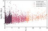 |
Fig. 1. Stellar mass as a function of redshift for the JADES sample (grey dots) and the selected galaxies studied in this work. Colours highlight the three redshift bins analysed in this work. |
3. A non-parametric star formation history tailored for early galaxies
The physical properties and SFH reconstruction were obtained through SED modelling of the JADES 23 photometric bands using the code CIGALE1 (Boquien et al. 2019). We included a non-parametric SFH module adapted for galaxies at high redshifts.
3.1. The SED modelling procedure
CIGALE is a public and versatile code that models galaxy SEDs from UV to radio taking into account the balance between the energy absorbed by dust in the UV-optical and re-emitted in the IR. The code can be used to fit photometry and spectroscopy, or to create mock SEDs thanks to its large library of models. CIGALE has been extensively tested, and a comparison with other SED modelling codes can be found in Pacifici et al. (2023). In this work we use a non-parametric SFH assumption, the stellar population models of Bruzual & Charlot (2003), and a Calzetti et al. (2000) dust attenuation law, which is found to be suitable for early galaxies (Bowler et al. 2022). We include nebular emission lines using a grid of CLOUDY simulations (Villa-Vélez et al. 2021). As output, the code provides a Bayesian-like analysis of each derived parameter.
3.2. Star formation history modelling
To model the SFH, we started from the non-parametric approach2 described in Ciesla et al. (2023) and Arango-Toro et al. (2023). This module makes use of priors to handle the SFR in each time bin of the SFH (see e.g. Leja et al. 2019; Tacchella et al. 2020; Suess et al. 2022). In CIGALE, Ciesla et al. (2023) implemented and tested this approach using a bursty-continuity prior (Tacchella et al. 2020). With a set of simulated SFH of z ∼ 1 galaxies, they showed that this SFH model provides stellar masses closer to the true values compared to analytical SFHs, as well as more accurate SFRs. A consistent and extensive analysis using CIGALE fits of galaxies from hydrodynamical simulations will be presented in Arango-Toro et al. (in prep.). However, Narayanan et al. (2024) recently showed that these priors do not allow the recovery of highly stochastic SFHs expected in galaxies at z > 6, which impacts the measurement of physical properties such as the stellar mass. Their results showed that a Dirichlet prior, for instance, reaches a limit on the minimum stellar mass that can be derived, while other priors, such as a rising one or a prior dedicated to post-starburst galaxies, provides underestimated stellar masses. There is a general consensus that different SFH priors lead to different results, and that there is not one prior adapted to all types of galaxies at any redshift (e.g. Leja et al. 2019; Suess et al. 2022). Furthermore, the non-parametric SFHs implemented in CIGALE, and also in PROSPECTOR (Johnson et al. 2021) or BAGPIPES (Carnall et al. 2018), make use of logarithmic binning of time. Although this binning is adapted for galaxies with ages of a few billion years, when galaxies are young (< 1 Gyr), such an approach might not be needed anymore.
We propose in this work a SFH modelling adapted for early galaxies with ages younger than 1 Gyr. We implemented, tested, and used a non-parametric SFH with linear time binning and a flat prior. The aim of this approach is to have a SFH flexible enough to capture possible bursts or stochastic activity, while providing a good estimate of properties like the stellar mass and SFR. In each bin, except the latest one (i.e. the closest to the time of observation), the SFR is randomly picked in a uniform distribution ranging from 0 to SFRmax, an input parameter of the code. To allow as much flexibility as possible in order to recover the right SFR, the latest bin is randomly picked in a log-uniform distribution, ranging from 10−2 to SFRmax. The assumed SFH is thus a set of ten bins linearly defined (the age of the galaxy divided in ten equal time bins) except for the latest one, which has an imposed duration of 10 Myr to be able to capture the most recent variation in star formation activity. This value is an input parameter and can be modified, as can the number of bins. For each input age parameter, a set of ten bins is thus defined with equal duration (except for the latest one).
To test our SFH model, we used the set of 32 simulated SFHs presented in Narayanan et al. (2024). They analysed two cosmological simulations at z ∼ 7 with significantly different stellar feedback models, and therefore dramatically different SFHs. In detail, they studied the SIMBA simulation (Davé et al. 2019), as well as a newly run simulation with the SMUGGLE feedback model (Marinacci et al. 2019). The former has a smoother rising star formation history, as is typical in cosmological simulations with artificially pressurised ISM models, while the latter is more bursty owing to the explicit feedback scheme. Narayanan et al. (2024) employed these two models with diverse star formation histories to analyse the ability of non-parametric SFH models in SED fitting in recovering the true stellar masses, and found that outshining from the most recent star formation (at the time of observation) hampered the ability to accurately derive galaxy star formation histories (and therefore, stellar masses) at high z.
We followed the same approach as Narayanan et al. (2024) by reducing all sources of uncertainty in the fit to be able to attribute the possible discrepancies only to SFH recovering. We thus used CIGALE to create the SEDs from the SIMBA and SMUGGLE simulated SFHs using Bruzual & Charlot (2003) stellar population models and a Calzetti et al. (2000) dust attenuation law with an E(B − V)s of 0.08. These SEDs were integrated into the same set of filters available in JADES with which we associated errors of 20% for JWST/NIRCam bands and 50% for HST bands, which are representative of the average errors provided in the JADES catalogue. We note that CIGALE adds an additional 10% to these values to take into account model uncertainties.
We fit these mock fluxes with CIGALE, using four age values, and thus four sets of ten SFH bins. This test is purposely simple and designed to identify discrepancies that are only due to SFH recovery. The output stellar masses and SFRs are compared to the true values from the simulated galaxies in Fig. 2. There is a good correlation between recovered stellar masses and the true values with a small systematic offset of 0.07 dex. Instantaneous SFRs are well recovered. We conducted the same test using the bursty continuity prior and found consistent results, with good estimates of the stellar masses and SFRs of the SEDs built from the SMUGGLE and SIMBA simulated SFHs.
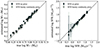 |
Fig. 2. Constraints on stellar masses and SFRs using the non-parametric SFH with flat prior. Left panel: stellar mass recovered with CIGALE using the non-parametric SFH with no prior vs the true stellar mass of the simulated SEDs. The light green dots indicate data points obtained using a non-parametric SFH with bursty continuity prior, while the dark green dots are data points obtained with the non-parametric SFH without prior proposed in this work. In this simple test procedure, the errors on the stellar mass are smaller than the size of the circles. Right panel: same as the left panel, but for the SFR. |
To evaluate the quality of the SFH reconstruction, we compared the SFR recovered in each time bin to the true values in Fig. 3. To this end, we projected the SFHs from simulations on the same time grid used by CIGALE. Results show a better recovery of the SFH by the model with a flat prior compared to the bursty continuity prior, at least up to the fifth bin going in lookback time: the median systematic offset of the recovered SFR in the different bins is −0.05 for the flat prior model and 0.33 for the bursty continuity prior. Although both priors provide good estimates of both stellar masses and SFRs, the difference in SFH reconstruction seen in Fig. 3 is explained by the difference in age estimate provided by these two models. The bursty continuity prior yields lower formation ages, that is the age at which the galaxy has formed 50% of its stellar mass. At an earlier time in the life of the galaxy the SFH is still recovered, but the comparison is more dispersed. We used the results of this test to calibrate our fitting procedure, and provide the input set of parameters used to run CIGALE in Table 1. This parameter set results in the best compromise to cover the JADES observed colours, while ensuring a reasonable number of models for computing reasons.
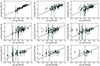 |
Fig. 3. Comparison between the simulated SFHs from Narayanan et al. (2024), binned as the CIGALE non-parametric SFHs, and the recovered SFR in the same time bins obtained with CIGALE. Bin 1 corresponds to the latest bin, at time of the observation, while bin 9 corresponds to the earliest time bin. The light green dots are obtained using a non-parametric SFH with bursty continuity prior while the dark green dots are obtained with the non-parametric SFH without prior proposed in this work. |
CIGALE input parameters used to fit the JADES sample.
4. Early galaxies on the SFR–M* plane
We place the JADES galaxies of our sample in the SFR–M* plane, using the instantaneous SFR and separating the three redshift bins (Fig. 4). The grey shaded regions are a limit implied by the non-parametric models in CIGALE, which cannot reach such high specific SFRs (sSFR). However, this upper limit is sensible for our study: Harikane et al. (2023) presented a sample of galaxies with redshifts between 8.8 and 13.2, spectroscopically confirmed, that have sSFRs ranging from 1.2 × 10⁻⁹ and 1.9 × 10⁻⁸ yr−1. The range of sSFR covered by CIGALE is also consistent with what is expected from simulations (Wilkins et al. 2023).
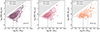 |
Fig. 4. SFR as a function of M* in three bins of redshift. The positions of JADES galaxies are indicated by the coloured points and contours. The grey dotted and dashed lines indicate where the sample is 95% and 85% complete, respectively. The grey regions indicate part of the SFR–M* plane not covered by the models used to do the SED fitting. |
4.1. Sample completeness
To determine the mass completeness of the sample studied in this work, we used the method described in Pozzetti et al. (2010, see also Florez et al. 2020; Mountrichas et al. 2022). We calculated the limiting stellar mass, that is the mass that a galaxy would have if its magnitude were equal to the limiting magnitude of the survey: log M*, lim = log M* + 0.4 × (mAB − mAB, lim). For this, we used the NIRCam/F200W filter and the flux sensitivity of 4.4 nJy provided in Rieke et al. (2024). We then selected the 20% faintest galaxies of the sample and calculated the limiting masses at the 95th and 85th percentiles of this distribution. The sample is 95% complete above log(M*, lim/M⊙) = 8.08, 8.19, and 8.63, at 6 < z < 7, 7 < z < 9, and 9 < z < 12, respectively, and 85% complete above log(M*, lim/M⊙) = 7.60, 7.74, and 7.99, in the same redshift bins. As a second step, we computed the SFR above which our sample is complete, using the same procedure as for the stellar mass. The 95% completeness reached at log(SFRlim/M⊙ yr−1) is −0.34, −0.24, and −0.22 at 6 < z < 7, 7 < z < 9, and 9 < z < 12, respectively, while the 85% completeness is reached at −0.56, −0.48, and −0.51. These limits are indicated in Fig. 4.
4.2. SFR–M* correlation
In the 6 < z < 7 redshift bin, there is evidence for a relation between the SFR and stellar mass that is strengthened by the absence of galaxies with strong SFR compared to the main population. This limit is not induced by the models used to perform the SED fitting that allow us to reach all the white parts of the SFR–M* planes shown in Fig. 4. In the 7 < z < 9 redshift bin, we see a relation between the SFR and the stellar mass that is broader than in the previous redshift bin. Finally, in the highest redshift bin, 9 < z < 12, there is no clear evidence for a relationship between SFR and M*. Instead, although it shows some dispersion, the SFR seems to be constant as a function of stellar mass. Only at high masses (log M* ≳ 9) does the SFR of the few galaxies at these masses seem to increase with M*. At these high redshifts, the SFR seems to be insensitive to the stellar mass of the galaxy. To test whether this effect could be due to a bias in estimating the stellar mass, given the rest-frame wavelength coverage of our sample, we removed the longest NIRCam filters of the SEDs of z ∼ 8 galaxies to mimic the rest-frame coverage of the galaxies in the highest redshift bin. The stellar masses obtained with this narrower wavelength range are consistent with those obtain with the full filter set, with a ratio of 1.10 ± 0.23 between the two stellar masses estimates. We conclude that, with the data in hand, the constant SFR distribution observed as a function of stellar mass at 9 < z < 12 is not due to stellar mass bias linked to rest-frame wavelength coverage.
To characterise the relationship between the SFR and stellar mass seen in Fig. 4, we computed the Spearman coefficient as an indicator of its strength. We varied the minimum stellar mass considered in the subsamples, and show the results of this test in Fig. 5, where only Spearman coefficients estimated with a p-value lower than 0.05 are shown. Using the different mass thresholds, the derived coefficients range from 0.15 to 0.5. At 6 < z < 7, the Spearman coefficient, when considering the sample above log M* = 7.5, is 0.48 corresponding to a strong relationship between the SFR and the stellar mass parameters (Dancey & Reidy 2004). At 7 < z < 9, the results indicate a moderate relationship when considering the same threshold. For the highest redshift bin (9 < z < 12), the Spearman coefficient values only indicate a moderate or strong relationship between the two parameters for high masses, that is above log M* = 8.5. At these high redshifts, when considering all sources, there is only weak evidence for it. The observations made in Fig. 4 are confirmed by the Spearman coefficient analysis, highlighting a strong relationship between the SFR and stellar mass at z < 7 that slightly weakens at 7 < z < 9. At higher redshifts, the relation is strong only for the most massive galaxies.
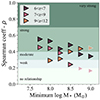 |
Fig. 5. Spearman coefficient of the SFR vs stellar mass as a function of the minimum stellar mass used to compute it. The symbol colours indicate the redshift range of the galaxies considered. Those with black contours are considered reliable coefficient values since they are associated with p-values lower than 0.05. The green shaded regions indicate the interpretation scale. |
We compare our SFR–M* relations with samples of early galaxies available in the literature in Fig. 6, converting all masses and SFR to Salpeter (1955) initial mass function (IMF). There is a good agreement between our relations and observed sources presented in the literature when comparing with our 6 < z < 7 and 7 < z < 9 redshift bins, although we estimate slightly lower SFR at a given mass. This can be due to different selections between our sample and those of the literature that were generally obtained through specific criteria (e.g. colour diagrams, spectroscopic observations). However, we observed a flatter relation for our highest redshift bin (9 < z < 12), which falls off with a slope of 0.64. Although built with a small sample size, we give the median SFR of galaxies with log M* ∼ 9.5 as an indication, but we do not use this point in the fit. We add for comparison predictions from the models of Yung et al. (2024) and the Sphinx simulations Katz et al. (2023). In the case of the Sphinx simulations, we note that, above log M* = 8.5, the normalisation of their relation increases with increasing redshift, while we observe the opposite with our data.
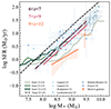 |
Fig. 6. SFR as a function of stellar mass. The relations found in the redshift bins studied in this work are shown with the solid lines and shaded regions. They are compared to samples in the literature. The relations from the simulations are shown as the dashed black (Yung et al. 2019) and solid green lines (Katz et al. 2023). The SFR and masses from the literature have been converted to a Salpeter (1955) IMF dividing by 0.63 from a Chabrier (2003) IMF or by 0.67 from a Kroupa & Boily (2002) IMF (Madau & Dickinson 2014; Bernardi et al. 2018). |
5. From stochastic to continuous SFH
In this section we characterise the SFH of galaxies; we denote as stochastic a SFH where the SFR at a given time bin, defined in Sect. 3, is independent from the SFR of the previous time bin, or in other words, where it cannot be predicted from the SFR of the previous bin. With this stochasticity, we expect to see galaxies going up and down on the SFR–M* plane with no coherent movement. This is opposed to the concept of secularity implied by the MS for which knowing the SFR at a given stellar mass allows the SFR of the next stellar mass bin to be predicted. When on the MS, we still expect galaxies to exhibit a certain level of stochasticity (e.g. Tacchella et al. 2016; Ciesla et al. 2023), but within the common flow that builds the MS.
We use the SFR gradient (∇SFR) proposed in Ciesla et al. (2023) to probe the movement of a galaxy in the SFR–M* plane and provide a dynamical approach of the MS. The SFR gradient is an angle (degree) relative to a constant SFR line in the SFR–M* plane that can be computed over different timescales. It involves the difference of the log SFR determined at the time of observation and at a given time in the past, as well as the stellar mass created during the same time. Tested and used in Ciesla et al. (2023) and Arango-Toro et al. (2023), it is an indicator of the recent SFH of galaxies. As shown in the left panel of Fig. 7, a galaxy with a strong positive ∇SFR is undergoing a starburst event and is going up on the SFR–M* plane while a galaxy with a strong negative gradient is undergoing a rapid and drastic quenching and is going down in the plane. This parameter, like the other parameters derived by CIGALE, is estimated through PDF analysis.
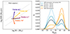 |
Fig. 7. Interpretation of the SFR gradient. Left panel: schematic example of the definition of ∇SFR. The gradient corresponding to each arrow is indicated in the same colour and shows the path that the galaxies followed recently. The point of the arrow indicates the position of the galaxy when observed. The black line is the reference from which the angle of the gradient is computed. The grey dashed lines give the position of the MS with its dispersion. Right panel: mock distributions of ∇SFR obtained from simple modelling. |
To help with the interpretation of ∇SFR and its distribution from a galaxy population, we compute mock ∇SFR assuming two cases. The first case is when galaxies have a completely stochastic SFH. We thus assume a flat prior on the SFR that a galaxy with log M* = 8 can reach between −0.2 < logSFR < 0.5, compatible with the SFR spread observed in Fig. 4 at this stellar mass. We show the resulting distributions in the right panel of Fig. 7. The distribution of galaxies with a completely stochastic SFH, within the boundaries set in our assumptions, is centred around 0° and spreads between −20° and 20°. In the second case we assume that the SFR of the mock galaxies can only follow the relation characterised in Fig. 6 assuming a 0.5 dex dispersion. In this case a slightly narrower distribution is observed peaking around ∇SFR = 45°. The distributions of these two scenarios thus have very different characteristics. In the same figure we show composite distributions to illustrate how mixed populations (composed of both stochastic and secular SFH galaxies) affect the gradient distributions.
We now compute the gradient distribution of our JADES galaxies to probe the variety of their SFHs. In Fig. 8, we show this distribution computed over the last 100 Myr in each redshift bin, and for different stellar mass bins.
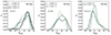 |
Fig. 8. Distribution of ∇SFR computed over 100 Myr in the three redshift bins. The different colours indicate the different stellar mass bins. |
At 6 < z < 7, almost all galaxies show a peak around 40° that is compatible with what we expect from galaxies following the flow of MS. However, galaxies with log M* between 7.8 and 8.2 have a broader distribution of ∇SFR from −20° to 45°. This indicates that a large fraction of low-mass galaxies tend to have stochastic star formation activity. With increasing stellar mass, the broad distribution changes with the increasing dominance of the peak at high positive values of ∇SFR. For the highest stellar mass bin (log M* between 9.1 and 9.5), the distribution has one peak around 40° and is slightly skewed towards lower gradient values. According to the mock distributions of Fig. 7, this indicates a dominance of galaxies with secular star formation that follow the flow of the MS, discussed in the previous section, with a small contribution from galaxies with stochastic SFH.
We repeat this analysis in the two other redshift bins. The 7 < z < 9 bin reveals that the galaxy population shows a broad double-peaked distribution of ∇SFR. For the highest mass bin (log M* between 8.6 and 9.1) the peak at high ∇SFR values, around 40°, is seen, but it is less prominent than in the lower redshift bin. A second peak appears around 5°, which is consistent with stochastic activity, as shown in Fig. 7. In the lowest mass bin the same type of distribution with the peak around low gradient values (∼10°) starts to be dominant compared to the MS gradient peak around 40°. As observed in the lower redshift bin, at low mass, the SFH of galaxies is predominantly stochastic.
Finally, in the 9 < z < 12 redshift bin, the ∇SFR distribution of the two stellar mass bins is clearly peaked around 0° with a weak secondary peak around 30−40°. The dominant peak is clearly compatible with a stochastic SFH drawn from a narrow SFR range, as shown in purple in Fig. 7. This strongly suggests that the dominant SFH type is stochastic at this redshift with a small part of massive galaxies that are compatible with secular star formation mode.
In Appendix A we show how the results deduced from Fig. 8 would be affected by degrading the constraint on ∇SFR. The main characteristics discussed in this section are recovered even assuming an error following a normal distribution with σ∇SFR = 20° (Fig. A.1).
In the gradient distribution of Fig. 8, the transition between the stochastic and continuous SFH seems to happen at stellar masses lower than 8.6 in the 6 < z < 7 and 7 < z < 9 redshift bins. This transition mass is expected from simulations. For instance, in their sample of galaxies from FIRE-2 zoom-in simulations (Hopkins et al. 2018), Ma et al. (2018) observed a large scatter in their MS relation at masses lower than log M* = 8 (with Kroupa 2001 IMF, thus ∼8.2 in Salpeter 1955 IMF) due to stronger burstiness in the SFHs. Consistent results obtained from simulations were also found by Dayal et al. (2013) and Kimm & Cen (2014). Using observations of local analogues of early galaxies, Emami et al. (2019) studied the distribution of the Hα-to-UV luminosity ratio as a proxy of burstiness and found its distribution to be larger in galaxies with log(M*/M⊙) < 8 (with Chabrier 2003 IMF, thus ∼8.2 in Salpeter 1955 IMF). These transition masses are consistent with what we observe with the JADES sample for which the median error of the stellar mass is 0.4 dex. Above log M* ∼ 9, galaxies with redshift between 6 and 7 show SFHs that are compatible with the majority of them following the MS.
6. Discussion
6.1. Star formation mode
Several studies, based on simulations (e.g. Dayal et al. 2013; Kimm & Cen 2014; Ma et al. 2018; Legrand et al. 2022; Gelli et al. 2023; Sun et al. 2023; Wilkins et al. 2023) and on observations (e.g. Faisst et al. 2019; Emami et al. 2019; Dressler et al. 2024; Looser et al. 2023), have shown that early galaxies had bursty or stochastic SFHs. In this work we reach a consistent conclusion for galaxies at z ≳ 9 through the analysis of their SFR gradients computed over the last 100 Myr. At lower redshift we see the emergence of galaxies with a gradient distribution compatible with a rising SFH and with a coherent movement of galaxies following the flow of the main sequence. To understand this transition between the star formation mode of galaxies at z ∼ 9, we show in Fig. 9 the fraction of massive (log M* > 9) galaxies that have a gradient compatible with a stochastic SFH and the fraction of massive galaxies following the flow of the MS with a gradient distribution peaking around 30−40°. There is a clear transition occurring between z = 7 and z = 9, thus in ∼200 Myr, where the majority of galaxies have a stochastic SFH at z > 9 (more than 80%), while at z ≲ 7 galaxies having a secular star formation mode dominate the population of massive galaxies. In Fig. A.2 we show how the results in Fig. 9 are affected by a weaker constraint on the ∇SFR estimates, and found no differences in our conclusions.
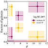 |
Fig. 9. Fraction of galaxies in the secular SFH gradient distribution (peak around 40°, yellow squares) and in the stochastic SFH distribution (peak around 0°, purple circles) as a function of redshift. |
6.2. Impact on UV emission and variability
The JWST Early Release Science results have highlighted an overabundance of galaxies at z = 10 and higher, probed by the UVLF (e.g. Harikane et al. 2023; Finkelstein et al. 2023). Several explanations have been proposed to understand this overabundance with physical processes involving the median level of UV emission (Inayoshi et al. 2022; Ferrara et al. 2022; Dekel et al. 2023; Mason et al. 2023; Yung et al. 2024) or its stochasticity (Mason et al. 2023; Mirocha & Furlanetto 2023; Shen et al. 2023).
The stochasticity of star formation has been quantified in the literature with σUV, the dispersion in mag around a median MUV obtained from a MUV − Mhalo relation. Shen et al. (2023) proposed three sources of variability that would impact σUV and that could, all together, contribute significantly to this excess of UV emission seen in the UVLF. They first consider the halo assembly, which is the mass accretion rate of dark matter halos that follows a log-normal distribution with a typical σDM of ∼0.3 dex (e.g. Mirocha & Furlanetto 2023). Then they consider the effect of dust attenuation, either through geometrical distribution or the effect of radiative feedback from star formation burst on the dust content (e.g. Ferrara et al. 2022). Based on their adopted AUV − β relation they estimate a dispersion due to dust, σdust, of ∼0.7 dex. Finally, the third possible cause of variability is star formation activity such as that discussed in our study, and they adopt a conservative value of σSF of ≥0.3 dex corresponding to the scatter of the MS at lower redshift. The three σ values considered together constitute σUV, which they estimate to vary from 0.75 mag at the bright end of the UVLF to 1.5 mag at the faint end, at z ∼ 9.
Using our sample, we derived the dispersion of the absolute magnitude MUV distribution, σUV, computed from a rest-frame wavelength window between 145 and 155 nm using our SED fitting run. Our derived σUV are shown in Fig. 10 as a function of redshift. Considering that stellar mass traces the halo mass, we computed the MUV distribution in between log(M*/M⊙) = 8 (8.5 at 9 < z < 12), the 95% completeness mass limit, and log M* = 9.5. These results in UV magnitude are in the ranges of −16.5 > MUV > −18.9, −16.3 > MUV > −18.6, and −16.6 > MUV > −18.4, at 6 < z < 7, 7 < z < 9, and 9 < z < 12, respectively. In all redshift bins we find σUV of 1.2 ± 0.1 mag. Subdividing the stellar mass bins results in consistent estimates.
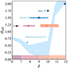 |
Fig. 10. σUV as a function of redshift. Estimates from the literature, based on simulation and theoretical approaches, are shown in shades of blue. |
Following the same approach as used in Shen et al. (2023), we decomposed our σUV into the three components. We cannot probe the variation of DM accretion rate with our data and thus use the same value as Shen et al. (2023) (i.e. 0.3 dex). Regarding the effect of dust, we derive from our SED modelling the distribution of attenuation in the same rest-frame band used to derive MUV and obtain ∼0.35 mag, depending on the redshift bin. Finally, we estimated the observed dispersion of the galaxies in the SFR–M* plane and obtained ∼0.5 dex in the considered stellar mass bin. Combining these, we obtained a σUV of 0.68 mag which is lower than our observed MUV based σUV.
Our σUV are compared to estimates from the literature in Fig. 10. Pallottini & Ferrara (2023) used the SERRA simulations and estimated a σUV of 0.61 mag from a sample of 245 simulated galaxies at z ∼ 7.7 studying the time-dependant variation of the SFR over averaged SFR, an indicator of burstiness. They concluded that, from their simulations, the SFR variations cannot account for the required z ≳ 10 boost in UVLF. Although their estimated σUV is lower than ours, our analysis reaches consistent conclusions. Muñoz et al. (2023) used semi-empirical models that allowed us to derive the expected evolution of σUV finding low values (< 0.8 mag) up to z ∼ 10, followed by a strong and rapid increase up to 2 mag at z ∼ 11. There is a strong increase in their predicted σUV over the 9 < z < 12 range that could be compatible with our estimate. With a different approach, Mason et al. (2023) used empirical models to study the distribution of the MUV − Mhalo relation and showed that young-aged galaxies significantly upscatter UV emission up to 1.5 mag above the median relation. Although within the range proposed by Mason et al. (2023), our σUV values derived from observations and SED modelling are lower than the estimates from Shen et al. (2023). This level of stochasticity is not sufficient to explain the excess of UV emission seen from the UVLF.
7. Conclusions
We have used a subsample of galaxies at 6 < z < 12 from the JADES public catalogue (Rieke et al. 2024) to investigate the variability of star formation at these redshifts. As the star formation activity is expected to be highly stochastic at these high redshifts, we have implemented in CIGALE a non-parametric SFH built with a linear sampling of time and no imposed prior. Tested on the simulated galaxies studied in Narayanan et al. (2024), we have found that although the usual bursty continuity prior recovers the stellar mass and SFR of the simulated galaxies well, the proposed parametrisation using linear bins and no prior provides a better reconstruction of the SFH. We therefore used this approach, fitted the JADES galaxies with CIGALE, and reached the following conclusions:
-
We observe a strong relationship between the SFR and stellar mass in the 6< z< 7 redshift range that weakens in the 7< z< 9 redshift bin. There is no strong evidence for a link between SFR and stellar mass at z> 9 for low-mass galaxies with, instead, a rather flat SFR distribution as a function of stellar mass. The few massive (log M*≳9) galaxies at this high redshift bin gives a hint of a stronger relationship between SFR and M*.
-
We use the SFR gradient, an indicator of the movement of galaxies in the SFR–M* plane, and thus directly linked to the galaxies’ SFH. Computed over 100 Myr, the gradient distribution shows an evolution with redshift for the most massive galaxies (log M* ≳ 9): the peaked distribution centred around 40°, expected from a secular star formation activity of galaxies following the flow of the MS, fades with increasing redshift, whereas the peaked distribution centred around 0°, consistent with a stochastic SFH, increases with increasing redshift. The transition between the prominence of secular star formation mode and the stochastic SFH mode occurs in the 7 < z < 9 redshift bin.
-
At 6 < z < 9, low-mass galaxies (log M* < 8.5) have stochastic SFH.
-
From our SED modelling, we derived the dispersion of the UV absolute magnitude MUV distribution and obtain σUV of 1.2 ± 0.1 mag in the three redshift bins. This value seems to be too low to explain the UV excess of the UVLF at high redshift from stochasticity of star formation only.
We observe a change in the star formation history of galaxies that is marked around z ∼ 9 (i.e. the redshift range where JWST makes a noticeable difference compared to previous instruments). In the most recent period (z < 9), galaxies have been found to dominantly form their stars in a secular star formation mode (i.e. with moderate oscillations of their SFR and with a strong correlation with their stellar mass). This mode breaks down around 550 Myr after the big bang (z ∼ 9). At earlier epochs, a more stochastic mode of star formation dominates with on and off star formation phases until galaxies reach a critical mass and enter in a more secular star formation phase putting them on the star formation main sequence. At z < 7, about 85% of the galaxies have reached the main sequence.
We note that despite this early stochastic period, the level of variation that we estimate remains below the very high stochasticity that would be needed to explain the excess of galaxies found in the UV luminosity function at z ≳ 10.
We recall, however, that our results are based on a limited rest-frame wavelength coverage at these very high redshifts where they rely on the quality of photometric redshifts. Future observations with the JWST will provide more material to investigate and quantify this transition further.
This CIGALE module is not available in the public version, but can be provided upon request.
Acknowledgments
L.C. thanks M. Boquien, as always, for useful discussions on CIGALE. The authors warmly thank the JADES team for the huge work and effort put in the preparation, observation, and production of the data used in this work. This project has received financial support from CNRS and CNES through the MITI interdisciplinary programs. We acknowledge the funding of the French Agence Nationale de la Recherche for the project iMAGE (grant ANR-22-CE31-0007). C.G.G. acknowledges support from CNES. NIRCam was built by a team at the University of Arizona (UofA) and Lockheed Martin’s Advanced Technology Center, led by Prof. Marcia Rieke at UoA. This work is based on observations made with the NASA/ESA/CSA James Webb Space Telescope. The data were obtained from the Mikulski Archive for Space Telescopes at the Space Telescope Science Institute, which is operated by the Association of Universities for Research in Astronomy, Inc., under NASA contract NAS 5-03127 for JWST.
References
- Arango-Toro, R. C., Ciesla, L., Ilbert, O., et al. 2023, A&A, 675, A126 [NASA ADS] [CrossRef] [EDP Sciences] [Google Scholar]
- Arrabal Haro, P., Dickinson, M., Finkelstein, S. L., et al. 2023, ApJ, 951, L22 [NASA ADS] [CrossRef] [Google Scholar]
- Bernardi, M., Sheth, R. K., Fischer, J. L., et al. 2018, MNRAS, 475, 757 [NASA ADS] [CrossRef] [Google Scholar]
- Boquien, M., Burgarella, D., Roehlly, Y., et al. 2019, A&A, 622, A103 [NASA ADS] [CrossRef] [EDP Sciences] [Google Scholar]
- Bowler, R. A. A., Cullen, F., McLure, R. J., Dunlop, J. S., & Avison, A. 2022, MNRAS, 510, 5088 [NASA ADS] [CrossRef] [Google Scholar]
- Brammer, G. B., van Dokkum, P. G., & Coppi, P. 2008, ApJ, 686, 1503 [Google Scholar]
- Bruzual, G., & Charlot, S. 2003, MNRAS, 344, 1000 [NASA ADS] [CrossRef] [Google Scholar]
- Bunker, A. J., Cameron, A. J., Curtis-Lake, E., et al. 2023, A&A, submitted [arXiv:2306.02467] [Google Scholar]
- Calzetti, D., Armus, L., Bohlin, R. C., et al. 2000, ApJ, 533, 682 [NASA ADS] [CrossRef] [Google Scholar]
- Carnall, A. C., McLure, R. J., Dunlop, J. S., & Davé, R. 2018, MNRAS, 480, 4379 [Google Scholar]
- Chabrier, G. 2003, PASP, 115, 763 [Google Scholar]
- Ciesla, L., Gómez-Guijarro, C., Buat, V., et al. 2023, A&A, 672, A191 [NASA ADS] [CrossRef] [EDP Sciences] [Google Scholar]
- Curtis-Lake, E., Carniani, S., Cameron, A., et al. 2023, Nat. Astron., 7, 622 [NASA ADS] [CrossRef] [Google Scholar]
- Daddi, E., Dickinson, M., Morrison, G., et al. 2007, ApJ, 670, 156 [NASA ADS] [CrossRef] [Google Scholar]
- Dancey, C., & Reidy, J. 2004, in Statistics without Maths for Psychology: Using SPSS for Windows, ed. E. Harlow (Pearson/Prentice Hall), 3 [Google Scholar]
- Davé, R., Anglés-Alcázar, D., Narayanan, D., et al. 2019, MNRAS, 486, 2827 [Google Scholar]
- Dayal, P., Dunlop, J. S., Maio, U., & Ciardi, B. 2013, MNRAS, 434, 1486 [NASA ADS] [CrossRef] [Google Scholar]
- De Barros, S., Oesch, P. A., Labbé, I., et al. 2019, MNRAS, 489, 2355 [NASA ADS] [CrossRef] [Google Scholar]
- Dekel, A., Sarkar, K. C., Birnboim, Y., Mandelker, N., & Li, Z. 2023, MNRAS, 523, 3201 [NASA ADS] [CrossRef] [Google Scholar]
- Donnan, C. T., McLeod, D. J., Dunlop, J. S., et al. 2023, MNRAS, 518, 6011 [Google Scholar]
- Dressler, A., Rieke, M., Eisenstein, D., et al. 2024, ApJ, 964, 150 [NASA ADS] [CrossRef] [Google Scholar]
- Eisenstein, D. J., Willott, C., Alberts, S., et al. 2023, ApJS, submitted [arXiv:2306.02465] [Google Scholar]
- Elbaz, D., Daddi, E., Le Borgne, D., et al. 2007, A&A, 468, 33 [NASA ADS] [CrossRef] [EDP Sciences] [Google Scholar]
- Emami, N., Siana, B., Weisz, D. R., et al. 2019, ApJ, 881, 71 [NASA ADS] [CrossRef] [Google Scholar]
- Endsley, R., Stark, D. P., Whitler, L., et al. 2023, MNRAS, submitted [arXiv:2306.05295] [Google Scholar]
- Faisst, A. L., Capak, P. L., Emami, N., Tacchella, S., & Larson, K. L. 2019, ApJ, 884, 133 [NASA ADS] [CrossRef] [Google Scholar]
- Ferrara, A., Sommovigo, L., Dayal, P., et al. 2022, MNRAS, 512, 58 [NASA ADS] [CrossRef] [Google Scholar]
- Finkelstein, S. L., Bagley, M. B., Ferguson, H. C., et al. 2023, ApJ, 946, L13 [NASA ADS] [CrossRef] [Google Scholar]
- Florez, J., Jogee, S., Sherman, S., et al. 2020, MNRAS, 497, 3273 [NASA ADS] [CrossRef] [Google Scholar]
- Gelli, V., Salvadori, S., Ferrara, A., Pallottini, A., & Carniani, S. 2023, ApJ, 954, L11 [NASA ADS] [CrossRef] [Google Scholar]
- Hainline, K. N., Johnson, B. D., Robertson, B., et al. 2024, ApJ, 964, 71 [CrossRef] [Google Scholar]
- Harikane, Y., Ouchi, M., Oguri, M., et al. 2023, ApJS, 265, 5 [NASA ADS] [CrossRef] [Google Scholar]
- Harikane, Y., Nakajima, K., Ouchi, M., et al. 2024, ApJ, 960, 56 [NASA ADS] [CrossRef] [Google Scholar]
- Hopkins, P. F., Wetzel, A., Kereš, D., et al. 2018, MNRAS, 480, 800 [NASA ADS] [CrossRef] [Google Scholar]
- Inayoshi, K., Harikane, Y., Inoue, A. K., Li, W., & Ho, L. C. 2022, ApJ, 938, L10 [NASA ADS] [CrossRef] [Google Scholar]
- Johnson, B. D., Leja, J., Conroy, C., & Speagle, J. S. 2021, ApJS, 254, 22 [NASA ADS] [CrossRef] [Google Scholar]
- Katz, H., Rosdahl, J., Kimm, T., et al. 2023, Open J. Astrophys., 6, 44 [NASA ADS] [CrossRef] [Google Scholar]
- Kimm, T., & Cen, R. 2014, ApJ, 788, 121 [NASA ADS] [CrossRef] [Google Scholar]
- Komatsu, E., Smith, K. M., Dunkley, J., et al. 2011, ApJS, 192, 18 [Google Scholar]
- Kroupa, P. 2001, MNRAS, 322, 231 [NASA ADS] [CrossRef] [Google Scholar]
- Kroupa, P., & Boily, C. M. 2002, MNRAS, 336, 1188 [Google Scholar]
- Labbé, I., Oesch, P. A., Bouwens, R. J., et al. 2013, ApJ, 777, L19 [CrossRef] [Google Scholar]
- Legrand, L., Hutter, A., Dayal, P., et al. 2022, MNRAS, 509, 595 [Google Scholar]
- Leja, J., Carnall, A. C., Johnson, B. D., Conroy, C., & Speagle, J. S. 2019, ApJ, 876, 3 [Google Scholar]
- Looser, T. J., D’Eugenio, F., Maiolino, R., et al. 2023, A&A, submitted [arXiv:2306.02470] [Google Scholar]
- Looser, T. J., D’Eugenio, F., Maiolino, R., et al. 2024, Nature, 629, 53 [Google Scholar]
- Ma, X., Hopkins, P. F., Garrison-Kimmel, S., et al. 2018, MNRAS, 478, 1694 [NASA ADS] [CrossRef] [Google Scholar]
- Madau, P., & Dickinson, M. 2014, ARA&A, 52, 415 [Google Scholar]
- Marinacci, F., Sales, L. V., Vogelsberger, M., Torrey, P., & Springel, V. 2019, MNRAS, 489, 4233 [NASA ADS] [CrossRef] [Google Scholar]
- Mason, C. A., Trenti, M., & Treu, T. 2023, MNRAS, 521, 497 [NASA ADS] [CrossRef] [Google Scholar]
- Mirocha, J., & Furlanetto, S. R. 2023, MNRAS, 519, 843 [Google Scholar]
- Mountrichas, G., Buat, V., Yang, G., et al. 2022, A&A, 663, A130 [NASA ADS] [CrossRef] [EDP Sciences] [Google Scholar]
- Muñoz, J. B., Mirocha, J., Furlanetto, S., & Sabti, N. 2023, MNRAS, 526, L47 [CrossRef] [Google Scholar]
- Naidu, R. P., Oesch, P. A., van Dokkum, P., et al. 2022, ApJ, 940, L14 [NASA ADS] [CrossRef] [Google Scholar]
- Narayanan, D., Lower, S., Torrey, P., et al. 2024, ApJ, 961, 73 [NASA ADS] [CrossRef] [Google Scholar]
- Noeske, K. G., Weiner, B. J., Faber, S. M., et al. 2007, ApJ, 660, L43 [CrossRef] [Google Scholar]
- Pacifici, C., Iyer, K. G., Mobasher, B., et al. 2023, ApJ, 944, 141 [NASA ADS] [CrossRef] [Google Scholar]
- Pallottini, A., & Ferrara, A. 2023, A&A, 677, L4 [NASA ADS] [CrossRef] [EDP Sciences] [Google Scholar]
- Pozzetti, L., Bolzonella, M., Zucca, E., et al. 2010, A&A, 523, A13 [NASA ADS] [CrossRef] [EDP Sciences] [Google Scholar]
- Qin, Y., Balu, S., & Wyithe, J. S. B. 2023, MNRAS, 526, 1324 [NASA ADS] [CrossRef] [Google Scholar]
- Rieke, M., Robertson, B., Tacchella, S., et al. 2024, ApJS, 269, 16 [Google Scholar]
- Roberts-Borsani, G. W., Bouwens, R. J., Oesch, P. A., et al. 2016, ApJ, 823, 143 [NASA ADS] [CrossRef] [Google Scholar]
- Robertson, B. E., Tacchella, S., Johnson, B. D., et al. 2023, Nat. Astron., 7, 611 [NASA ADS] [CrossRef] [Google Scholar]
- Salpeter, E. E. 1955, ApJ, 121, 161 [Google Scholar]
- Shen, X., Vogelsberger, M., Boylan-Kolchin, M., Tacchella, S., & Kannan, R. 2023, MNRAS, 525, 3254 [NASA ADS] [CrossRef] [Google Scholar]
- Smit, R., Bouwens, R. J., Labbé, I., et al. 2014, ApJ, 784, 58 [NASA ADS] [CrossRef] [Google Scholar]
- Suess, K. A., Leja, J., Johnson, B. D., et al. 2022, ApJ, 935, 146 [NASA ADS] [CrossRef] [Google Scholar]
- Sun, G., Faucher-Giguère, C.-A., Hayward, C. C., & Shen, X. 2023, MNRAS, 526, 2665 [NASA ADS] [CrossRef] [Google Scholar]
- Tacchella, S., Dekel, A., Carollo, C. M., et al. 2016, MNRAS, 458, 242 [NASA ADS] [CrossRef] [Google Scholar]
- Tacchella, S., Forbes, J. C., & Caplar, N. 2020, MNRAS, 497, 698 [Google Scholar]
- Tang, M., Stark, D. P., Chevallard, J., & Charlot, S. 2019, MNRAS, 489, 2572 [NASA ADS] [CrossRef] [Google Scholar]
- Villa-Vélez, J. A., Buat, V., Theulé, P., Boquien, M., & Burgarella, D. 2021, A&A, 654, A153 [NASA ADS] [CrossRef] [EDP Sciences] [Google Scholar]
- Wilkins, S. M., Vijayan, A. P., Lovell, C. C., et al. 2023, MNRAS, 518, 3935 [Google Scholar]
- Williams, C. C., Tacchella, S., Maseda, M. V., et al. 2023, ApJS, 268, 64 [NASA ADS] [CrossRef] [Google Scholar]
- Yung, L. Y. A., Somerville, R. S., Popping, G., et al. 2019, MNRAS, 490, 2855 [NASA ADS] [CrossRef] [Google Scholar]
- Yung, L. Y. A., Somerville, R. S., Finkelstein, S. L., Wilkins, S. M., & Gardner, J. P. 2024, MNRAS, 527, 5929 [Google Scholar]
Appendix A: Impact of the constraint on ∇SFR on the results
To understand how a weaker constraint of the SFR gradient would impact our results in Fig. 8, we perturbed the gradient estimates of the highest mass bin of each redshift range a thousand times, assuming different errors on ∇SFR. We perturbed the ∇SFR estimates by randomly peaking a value in a normal distribution with a σ of 5°, 10°, or 20°. As shown in Fig. A.1, the distributions broaden with increasing σ, but the position of the peaks is still clear and shows the two types of distribution that we interpret as galaxies with a stochastic SFH (∇SFR∼0°) and galaxies with a SFH following a coherent movement, indicative of secular star formation mode (∇SFR∼40°), even with σ = 20°. We repeated the same exercise to test the results given in Fig. 9 and reach the same conclusion (Fig. A.2). Even considering a high level of error of the estimate of ∇SFR, the transition between stochastic and secular star formation modes is still clear.
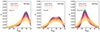 |
Fig. A.1. Distribution of ∇SFR computed over 100 Myr in the three redshift bins. The different colours indicate the different S/N values assumed to perturb the gradient distributions. |
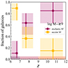 |
Fig. A.2. Fraction of galaxies in the secular SFH gradient distribution (peak around 40°, yellow squares) and in the stochastic SFH distribution (peak around 0°, purple circles), assuming that these distributions are normal, as a function of redshift. |
All Tables
All Figures
|
Fig. 1. Stellar mass as a function of redshift for the JADES sample (grey dots) and the selected galaxies studied in this work. Colours highlight the three redshift bins analysed in this work. |
| In the text | |
|
Fig. 2. Constraints on stellar masses and SFRs using the non-parametric SFH with flat prior. Left panel: stellar mass recovered with CIGALE using the non-parametric SFH with no prior vs the true stellar mass of the simulated SEDs. The light green dots indicate data points obtained using a non-parametric SFH with bursty continuity prior, while the dark green dots are data points obtained with the non-parametric SFH without prior proposed in this work. In this simple test procedure, the errors on the stellar mass are smaller than the size of the circles. Right panel: same as the left panel, but for the SFR. |
| In the text | |
|
Fig. 3. Comparison between the simulated SFHs from Narayanan et al. (2024), binned as the CIGALE non-parametric SFHs, and the recovered SFR in the same time bins obtained with CIGALE. Bin 1 corresponds to the latest bin, at time of the observation, while bin 9 corresponds to the earliest time bin. The light green dots are obtained using a non-parametric SFH with bursty continuity prior while the dark green dots are obtained with the non-parametric SFH without prior proposed in this work. |
| In the text | |
|
Fig. 4. SFR as a function of M* in three bins of redshift. The positions of JADES galaxies are indicated by the coloured points and contours. The grey dotted and dashed lines indicate where the sample is 95% and 85% complete, respectively. The grey regions indicate part of the SFR–M* plane not covered by the models used to do the SED fitting. |
| In the text | |
|
Fig. 5. Spearman coefficient of the SFR vs stellar mass as a function of the minimum stellar mass used to compute it. The symbol colours indicate the redshift range of the galaxies considered. Those with black contours are considered reliable coefficient values since they are associated with p-values lower than 0.05. The green shaded regions indicate the interpretation scale. |
| In the text | |
|
Fig. 6. SFR as a function of stellar mass. The relations found in the redshift bins studied in this work are shown with the solid lines and shaded regions. They are compared to samples in the literature. The relations from the simulations are shown as the dashed black (Yung et al. 2019) and solid green lines (Katz et al. 2023). The SFR and masses from the literature have been converted to a Salpeter (1955) IMF dividing by 0.63 from a Chabrier (2003) IMF or by 0.67 from a Kroupa & Boily (2002) IMF (Madau & Dickinson 2014; Bernardi et al. 2018). |
| In the text | |
|
Fig. 7. Interpretation of the SFR gradient. Left panel: schematic example of the definition of ∇SFR. The gradient corresponding to each arrow is indicated in the same colour and shows the path that the galaxies followed recently. The point of the arrow indicates the position of the galaxy when observed. The black line is the reference from which the angle of the gradient is computed. The grey dashed lines give the position of the MS with its dispersion. Right panel: mock distributions of ∇SFR obtained from simple modelling. |
| In the text | |
|
Fig. 8. Distribution of ∇SFR computed over 100 Myr in the three redshift bins. The different colours indicate the different stellar mass bins. |
| In the text | |
|
Fig. 9. Fraction of galaxies in the secular SFH gradient distribution (peak around 40°, yellow squares) and in the stochastic SFH distribution (peak around 0°, purple circles) as a function of redshift. |
| In the text | |
|
Fig. 10. σUV as a function of redshift. Estimates from the literature, based on simulation and theoretical approaches, are shown in shades of blue. |
| In the text | |
|
Fig. A.1. Distribution of ∇SFR computed over 100 Myr in the three redshift bins. The different colours indicate the different S/N values assumed to perturb the gradient distributions. |
| In the text | |
|
Fig. A.2. Fraction of galaxies in the secular SFH gradient distribution (peak around 40°, yellow squares) and in the stochastic SFH distribution (peak around 0°, purple circles), assuming that these distributions are normal, as a function of redshift. |
| In the text | |
Current usage metrics show cumulative count of Article Views (full-text article views including HTML views, PDF and ePub downloads, according to the available data) and Abstracts Views on Vision4Press platform.
Data correspond to usage on the plateform after 2015. The current usage metrics is available 48-96 hours after online publication and is updated daily on week days.
Initial download of the metrics may take a while.