| Issue |
A&A
Volume 699, July 2025
|
|
|---|---|---|
| Article Number | A6 | |
| Number of page(s) | 14 | |
| Section | Extragalactic astronomy | |
| DOI | https://doi.org/10.1051/0004-6361/202451742 | |
| Published online | 25 June 2025 | |
The mass-metallicity relation as a ruler for galaxy evolution: Insights from the James Webb Space Telescope
1
Scuola Normale Superiore, Piazza dei Cavalieri 7, 56126 Pisa, Italy
2
Dipartimento di Fisica “Enrico Fermi”, Università di Pisa, Largo Bruno Pontecorvo 3, Pisa I-56127, Italy
3
Center for Computational Astrophysics, Flatiron Institute, 162 5th Avenue, New York, NY 10010, USA
4
INAF-Osservatorio di Astrofisica e Scienza dello Spazio, via Gobetti 93/3, I-40129 Bologna, Italy
⋆ Corresponding author: This email address is being protected from spambots. You need JavaScript enabled to view it.
Received:
31
July
2024
Accepted:
9
May
2025
Abstract
Context. Galaxy evolution emerges from the balance between cosmic gas accretion, fueling star formation, and supernova feedback, regulating metal enrichment of the interstellar medium. Hence, the relation between stellar mass (M⋆) and gas metallicity (Zg) is fundamental to understanding the physics of galaxies. High-quality spectroscopic JWST data enable accurate measurements of both M⋆ and Zg up to redshift z ≃ 10.
Aims. Our aims are to understand (i) the nature of the observed mass-metallicity relation (MZR), (ii) its connection with the star formation rate (SFR), (iii) the role played by SFR stochasticity (flickering), and (iv) how it is regulated by stellar feedback.
Methods. We compared the MZR obtained by the JADES, CEERS, and UNCOVER surveys, which comprise about 180 galaxies at z ≃ 3 − 10 with 106 M⊙ ≲ M⋆ ≲ 1010 M⊙, with ≃200 simulated galaxies in the same mass range from the SERRA high-resolution (≃20 pc) suite of cosmological radiation-hydrodynamic simulations. To interpret the MZR, we developed a minimal, physically motivated model of galaxy evolution that includes: cosmic accretion, possibly modulated with an amplitude A100 on 100 Myr timescales; a time delay, td, between SFR and supernova feedback; and SN-driven outflows with a varying mass loading factor, ϵSN, which is normalized to the FIRE simulations predictions for ϵSN = 1.
Results. Using our minimal model, we find the observed “mean” MZR is reproduced for relatively inefficient outflows (ϵSN = 1/4), in line with findings from JADES. Matching the observed MZR “dispersion” across the full stellar mass range requires a delay time, td = 20 Myr, in addition to a significant modulation (A100 = 1/3) of the accretion rate. Successful models are characterized by relatively low flickering (σSFR ≃ 0.2), corresponding to a metallicity dispersion of σZ ≃ 0.2. Such values are close but slightly lower than predicted from SERRA (σSFR ≃ 0.24, σZ ≃ 0.3), clarifying why SERRA shows a flatter trend with respect to the observations and some tension, especially at M⋆ ≃ 1010 M⊙.
Conclusions. The MZR appears to be very sensitive to SFR stochasticity. The minimal model predicts that high root mean square values (σSFR ≃ 0.5) result in a “chemical chaos” (i.e. σZ ≃ 1.4), virtually destroying the observed MZR. As a consequence, invoking a highly stochastic SFR (σSFR ≃ 0.8) to explain the overabundance of bright, super-early galaxies would lead to inconsistencies with the observed MZR.
Key words: galaxies: formation / galaxies: high-redshift / galaxies: star formation
© The Authors 2025
 Open Access article, published by EDP Sciences, under the terms of the Creative Commons Attribution License (https://creativecommons.org/licenses/by/4.0), which permits unrestricted use, distribution, and reproduction in any medium, provided the original work is properly cited.
This article is published in open access under the Subscribe to Open model. This email address is being protected from spambots. You need JavaScript enabled to view it. to support open access publication.
1. Introduction
The baryon cycle plays a pivotal role in regulating the galaxy formation and evolution process through cosmic time. As cosmic gas accretes in the dark matter halo potential well, it can cool and eventually form stars; massive stars explode as supernovae, enriching the surrounding interstellar medium with metals, which can potentially be ejected from the galaxy. Therefore, key information regarding the star formation and enrichment history is encoded in the relation between stellar mass (M⋆) and gas metallicity (Zg), the so-called mass-metallicity relation (MZR), making it effectively a standard ruler for galaxy evolution (see Maiolino & Mannucci 2019, for a review). Over the past 20 years, it has become possible to measure the MZR from z ≃ 0 (Tremonti et al. 2004; Kirby et al. 2013; Andrews & Martini 2013) up to the beginning of cosmic noon (z ≃ 3, Erb et al. 2006; Maiolino et al. 2008; Zahid et al. 2011; Sanders et al. 2018; Curti et al. 2020), mostly by using the oxygen-to-hydrogen abundance ratio, [O/H], as a proxy for Zg. Locally, these observations have shown that Zg increases with stellar mass up to M⋆≃ 1010 M⊙, and that beyond that point it flattens. This can be understood as being due to the fact that low-mass galaxies are prone to metal ejection due to their shallower potential well, while massive galaxies can retain most of the metals they have produced (Ferrara 2008). In this view, galaxy evolution is guided by a “bathtub” equilibrium (Bouché et al. 2010; Dekel & Mandelker 2014), which determines the metallicity by balancing infall and outflows (Lilly et al. 2013). Further, observations have highlighted that Zg and M⋆ are tightly connected with the star formation rate (SFR) in the so-called fundamental mass-metallicity relation (FMR, Mannucci et al. 2010), which seems to be redshift-independent up to z ≃ 3 (Curti et al. 2020). Other factors such as galaxy size (Ellison et al. 2008) and molecular gas content (Bothwell et al. 2013) might also play some secondary role in connecting Zg to M⋆. The MZR evolution at z ≳ 4 has been predicted via semi-analytical models (Dayal et al. 2013; Zahid et al. 2014; Ucci et al. 2023) or cosmological simulations (Torrey et al. 2019; Liu & Bromm 2020; Langan et al. 2020; Wilkins et al. 2023; Casavecchia et al. 2024). Most models predict almost no evolution or a very weak redshift dependence for z > 3 (Ma et al. 2016; Kannan et al. 2022; Marszewski et al. 2024); some others suggest a breakdown of the relation at z ≳ 9 − 12 (Pallottini et al. 2014; Sarmento et al. 2018). Thanks to the exquisite spectroscopic capabilities of JWST, we can accurately infer Zg for galaxies well within the Epoch of Reionization (EoR, z > 6). At present, surveys like JADES (Bunker et al. 2024) and CEERS (Finkelstein et al. 2023) have provided metallicity measurements at z ≃ 3 − 10 (Curti et al. 2024) and z ≃ 4 − 10 (Nakajima et al. 2023), for a combined sample of about 170 galaxies in the 5 × 10⁶ M⊙≲ M⋆ ≲ 1010 M⊙ stellar mass range. These JWST observations suggest that the MZR is already in place in the EoR, albeit downshifted by 0.5 dex with respect to the local one. The evolution in the z ≃ 3 − 10 range is very mild, as relatively low-mass (M⋆≃ 109−10 M⊙) galaxies can be chemically mature (Zg ≃ 0.3 Z⊙) already at z ≃ 6. The MZR shows a root mean square (rms) dispersion σZ = 0.3 dex, and possibly a hint of flattening at z ≳ 6 (Curti et al. 2024). Furthermore, multiple line detections in the same target can be used to constrain abundance patterns of individual elements (Kobayashi & Ferrara 2024; Curti et al. 2025). Resolved observations are beginning to probe the presence of metallicity gradients up to z ≃ 8 (Venturi et al. 2024), which should provide deeper insights into the formation process of the galaxy and the history of the stellar mass buildup (see Vallini et al. 2024, for an ALMA perspective). Observations targeting lensed fields (Bezanson et al. 2024; Chemerynska et al. 2024a) are uncovering the metallicities of even the fainter galaxies (Chemerynska et al. 2024b), which is key in order to explore the infall and outflow interplay due to stellar feedback in the less massive objects. Importantly, using observations of lensed targets at z ≃ 3 − 9, Morishita et al. (2024) suggest that the 0.5 dex shift of normalization and the higher scattering1 (0.3 dex, see also Heintz et al. 2023) with regard to the local MZR can be caused by the high level of burstiness of the SFR expected in high-z galaxies (Pallottini & Ferrara 2023; Sun et al. 2023a). Indeed, as we move from the local Universe to high z (see Madau & Dickinson 2014; Dayal & Ferrara 2018; Förster Schreiber & Wuyts 2020, for reviews), galaxies are expected to become more bursty, as a consequence of the increase in the specific SFR (sSFR, González et al. 2010; Stark et al. 2013; Smit et al. 2014) combined with a decrease in size (Shibuya et al. 2015), which can make the stellar feedback more effective (Krumholz & Burkhart 2016) in maintaining a higher level of turbulence (Simons et al. 2017; Genzel et al. 2017). With the recent availability of JWST observations (Roberts-Borsani et al. 2022; Castellano et al. 2022; Finkelstein & Bagley 2022; Naidu et al. 2022; Treu et al. 2022; Adams et al. 2023; Atek et al. 2023; Donnan et al. 2023; Harikane et al. 2023; Santini et al. 2023), the time-varying stochastic SFR behavior (in short, flickering or burstiness), has been invoked as a possible mechanism (Mason et al. 2023; Mirocha & Furlanetto 2023; Shen et al. 2023; Sun et al. 2023a; Kravtsov & Belokurov 2024) to explain the overabundance of bright galaxies at z ≳ 10 (see Dekel et al. 2023; Ferrara et al. 2023, for alternatives). However, some works predict that the rms amplitude of the SFR variability falls short of explaining the said overabundance (Pallottini & Ferrara 2023). Thus, it is unclear if flickering alone can explain the phenomenon, particularly since the required high level of variability (Muñoz et al. 2023) is apparently not seen in the data (Ciesla et al. 2024). Studies of the SFR flickering have experienced a recent surge, as stochastic SFR variations can have an impact on our ability to observe distant galaxies (Sun et al. 2023b) and affect the possibility of detecting Population III stars (Vikaeus et al. 2022; Katz et al. 2023). In addition, the flickering can modify the UV spectral slopes of high-z galaxies and the escape fraction of ionizing photons (Gelli et al. 2024a), ultimately controlling the cosmic reionization history (Davies & Furlanetto 2016; Nikolić et al. 2024). Analyzing the amplitude and temporal variation in SFR flickering provides unique insights into the various feedback processes that regulate the formation and evolution of early galaxies (Pallottini & Ferrara 2023). On the one hand, high-amplitude and high-frequency flickering, on timescales shorter than the delay between SFR and SN explosions (≃20 − 40 Myr), are invoked (Gelli et al. 2023, 2024b, 2025) to explain the observed abrupt quenching of the SFR in M⋆ ≃ 109 M⊙ galaxies already at z ≃ 7 (Dome et al. 2024; Looser et al. 2024; Endsley et al. 2024). On the other hand, the presence of disks observed in M⋆≃ 109−10 M⊙ galaxies up to z ≃ 7 (Rowland et al. 2024; Fujimoto et al. 2024) implies a limited level of stochasticity, as otherwise the disk would be disrupted (Kohandel et al. 2024). In the present work, we aim to clarify the effects of SFR flickering and feedback regulation of high-z galaxies by using the MZR as a standard ruler. The paper is structured as follows. In Sect. 2 we present the SERRA cosmological radiation-hydrodynamic simulation suite and compare it with MZR observations from JADES, CEERS, and UNCOVER. To obtain a broad-brush interpretation of the complex, nonlinear effects shaping the MZR, in Sect. 3 we develop a minimal, single-zone model to give a physical interpretation to the observed MZR. In Sect. 4 we discuss the interpretation of different simulations suites by analyzing them in the light of the simplified view enabled by the minimal model (Sect. 4.1), also discussing its shortcomings (Sect. 4.2); conclusions are given in Sect. 5.
2. The mass-metallicity relation at high redshift
To study the MZR at high-z, firstly we adopted the data from SERRA, a suite of cosmological zoom-in simulations that follows the evolution of z ≳ 6 galaxies (Pallottini et al. 2022). In SERRA we used the code RAMSES (Teyssier 2002) to evolve dark matter (DM), gas, and stars. We enabled the module RAMSES-RT (Rosdahl et al. 2013) to track radiation on the fly by coupling it (Pallottini et al. 2019; Decataldo et al. 2019) with KROME (Grassi et al. 2014), in order to account for nonequilibrium chemistry up to H2 formation (Pallottini et al. 2017a). Stars are formed using a Schmidt (1959)–Kennicutt (1998) – like relation based on H2. Once formed, stars produce UV radiation that ionizes the gas, photo-dissociates H2, and builds a radiation pressure in the gas. Massive stars generate stellar winds and explode as SNe. Depending on the kind of feedback, energy injection in the gas can be of thermal (subject to radiative losses) and/or turbulent (later dissipated) nature (Pallottini et al. 2017b). In SERRA, metallicity is tracked as the sum of heavy elements. Adopting a ≃ 1.2 × 10⁴ M⊙ (≃ 20 pc) gas mass (spatial) resolution, with MUSIC (Hahn & Abel 2011) we initialized cosmological initial conditions2 generated at z = 100, and followed the evolution of galaxies down to z = 6 (and z = 4 for a subsample, see Kohandel et al. 2024). For this work, we selected ≃200 central SERRA galaxies at z = 7.7 with a stellar mass of 106 M⊙≲ M⋆ ≲ 1010 M⊙; we computed the gas metallicity as  by considering the total gas (Mg) and metal (MZ) mass contained within 3 stellar effective radii from the galaxy center, which is close to the gas half-mass radius3. Note that, for a more direct comparison with the observations, we should compute line and continuum emission from SERRA galaxies; then, we could infer M⋆ from synthetic SED fitting and combine the line emission to prepare metallicity calibrators. Such an approach would reduce potential mismatches due to uncertainties in using different calibrators (Curti et al. 2017; Chemerynska et al. 2024b), for example to relax the single zone model assumption (Marconi et al. 2024) and correct for biases in the comparison (Cameron et al. 2023), also avoiding potential issues in the M⋆ determinations (Narayanan et al. 2024), which can hinder a robust determination of the MZR and its intrinsic scatter (Strom et al. 2022). Without FIR data, metallicity can typically be inferred for galaxies showing emission lines either constraining the electron temperature (Vallini et al. 2021; Markov et al. 2022; Morishita et al. 2024) or that can be combined to derive classical metallicity calibrators (e.g. Curti et al. 2020). By definition, this is only a subset of star-forming galaxies. It has to be noted that for some mini-quenched or post-starburst galaxies (Endsley et al. 2024) metallicity estimates are also possible (Carniani et al. 2025). While the fidelity of the comparison with observations might be improved by selecting from our model only star-forming galaxies (and imposing a SFR lower limit to mimic a UV survey limit), the presence of lines for metallicity determination depends on assumptions such as the IMF type, the fraction of binaries (e.g. Veraldi et al. 2025), and dust attenuation (Gelli et al. 2023). These choices add extra uncertainty to the models; future dedicated work is needed to explore this issue. Also, while this kind of forward modeling approach is very powerful, and also allows for the preparation of novel observational strategies (Zanella et al. 2021; Rizzo et al. 2022), here it hinders the possibility of making a comparison with most of the other models, as the MZR is usually computed integrating metal, gas, and stellar masses; thus, we avoid it in the present work. The predictions for SERRA are plotted in Fig. 1, along with JWST data from Curti et al. (2024, JADES sample, Bunker et al. 2024), Nakajima et al. (2023, CEERS sample, Finkelstein et al. 2023), and Chemerynska et al. (2024b, UNCOVER sample, Bezanson et al. 2024), for a total of about 180 galaxies at z ≃ 3 − 10 with 106 M⊙≲ M⋆ ≲ 1010 M⊙. The bulk of SERRA galaxies are between 107 M⊙ ≲ M⋆ ≲ 109 M⊙; these galaxies have 10−1.5 Z⊙ ≲ Zg ≲ 10−0.5 Z⊙, which is broadly consistent with the observed JWST galaxies. However, at 107 M⊙ ≲ M⋆ ≲ 108 M⊙ some SERRA galaxies show Zg ≃ 0.25 dex higher than the observed values; moreover, for M⋆ ≃ 1010 M⊙, Zg is on average lower than observed, up to extreme cases of 0.5 dex. In general, SERRA galaxies show no clear MZR trend and their dispersion appears to be somewhat larger than the observed one. Interestingly, with respect to Nakajima et al. (2023) and Curti et al. (2024), the lensed galaxies from Chemerynska et al. (2024b) seem to indicate lower values of Zg at M⋆ ≲ 107 M⊙; the lensed data seems consistent with SERRA, but only a select number of simulated galaxies and observations are in that mass range. As is noted by Curti et al. (2024), the lack of a clear trend and the large scatter in the SERRA relation resembles the behavior of their 6 < z < 10 sample. However clear differences are present, such as the relatively metal-rich galaxies at M⋆≃ 108 M⊙ and low-metallicity galaxies at M⋆≃ 1010 M⊙. Further, the lack of a clear trend might be partially due to galaxy sample selection, as most of the SERRA data has 108 M⊙ ≲ M⋆ ≲ 109 M⊙ and only a small fraction of galaxies has M⋆ ≃ 107 M⊙. Thus, the observed galaxy mass range is not uniformly covered by SERRA galaxies, whose sample is drawn from a collection of zoom-in simulations focusing on M⋆ ≃ 1010 M⊙ galaxies and their close environment. Indeed, some of the M⋆≲ 109 M⊙ mass galaxies form in a highly pre-enriched environment, which explains their relatively high metallicities (Zg ≃ 10−0.5, see Gelli et al. 2020). Note that considering different redshift intervals4 yields qualitatively similar results. Thus, in summary, the normalization of the MZR of SERRA is roughly similar to the observed galaxies, but no trend (flat MZR) is clearly visible (Rowland et al. 2025) and some discrepancies are present, especially in the M⋆ ≃ 1010 M⊙ range. Similar (or larger) tensions are present also when a comparison with other models is performed. These can be noted; for example, from the fit obtained by the FIRE-2 simulations (Marszewski et al. 2024). FIRE-2 data are close to the observed Zg at M⋆≃ 109.5 M⊙, but the predicted slope of the MZR is different, and thus the tension with Nakajima et al. (2023), Curti et al. (2024) increases with decreasing M⋆. Finally, FIRE-2 galaxies present a much higher scatter5, which increases with decreasing stellar mass up to ≃1 dex at M⋆≃ 5 × 10⁷ M⊙ (for a clearer comparison, see later Fig. 5). An in-depth comparison between observations and simulations is presented in Curti et al. (2024), which, in addition to SERRA, considers the zoom-in simulations from FIRSTLIGHT (Langan et al. 2020, see Ceverino et al. 2017 for the main paper) and FIRE (Ma et al. 2016, see Hopkins et al. 2014), the IllustrisTNG cosmological simulations Torrey et al. (2019, see Pillepich et al. 2018), and the ASTRAEUS semi-analytical models (Ucci et al. 2023, see Hutter et al. 2021); as detailed in Curti et al. (2024), most simulations seem to reasonably match the Zg data at ≃109 M⊙ but have steeper slopes and underpredict the metallicities at lower M⋆. Interestingly, some of the models (e.g. Marszewski et al. 2024; Cueto et al. 2024) seem to be consistent with what was observed by Chemerynska et al. (2024b), which however have only eight targets, thus it is unclear if there is a change of slope of the MZR for M⋆≲ 107 M⊙. Indeed, the observational determination of the slope of the MZR seems still uncertain, e.g. it seems to change with redshift, as indicated by the different slopes resulting from the separate analysis of Curti et al. (2024) for the 3 < z < 6 and 6 < z < 10 samples.
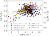 |
Fig. 1. Mass-metallicity relation (MZR) at high redshift (z). We plot the gas metallicity (Zg) as a function of stellar mass (M⋆) for the SERRA simulated galaxies (Pallottini et al. 2022, z ≃ 7) and the JWST observations from CEERS Nakajima et al. (2023, z ≃ 4 − 10), JADES (Curti et al. 2024, z ≃ 3 − 6 and 6–10), and UNCOVER (Chemerynska et al. 2024b, z ≃ 6 − 8). To guide the eye, the observational fits from Nakajima et al. (2023) and Curti et al. (2024) are also reported as lines with the same colors of corresponding data. As a reference, the log(Zg/Z⊙) = 0.37 log(M⋆/M⊙)−4.3 fit from FIRE-2 simulations (Marszewski et al. 2024, z = 5 − 12) is shown, along with their binned data and scatter at z = 8. The right axis reports the logarithmic oxygen abundance [O/H], assuming a solar composition (Asplund et al. 2009), i.e., 12 + [O/H]⊙ = 8.69. |
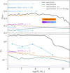 |
Fig. 5. SFR (σSFR, upper panel) and gas metallicity (σZ, lower panel) rms variations as a function of stellar mass for the sets of models presented in Fig. 4 (see Eqs. (3) for the definitions). As a reference, we report the SERRA average σSFR (Pallottini & Ferrara 2023) and σZ (this work), the σSFR from Ciesla et al. (2024), Mason et al. (2023), Muñoz et al. (2023), Shen et al. (2023), and the σZ for FIRE-2 at z = 8.0 (Marszewski et al. 2024) and JWST data. Note that ⟨JWST⟩ is the rms of the observations after subtraction of the fit to the MZR in the different datasets in Nakajima et al. (2023) and Curti et al. (2024); the thickness of the shaded area encloses the minimum and maximum of the rms of the different datasets. |
3. A minimal physical model to explain the MZR
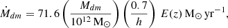
Given the very contrived match between simulations and observations, it seems worthwhile to step back and try to understand the trend and dispersion of the MZR using basic physical models. The advantage of the approach consists of simplifying the complexity of numerical simulation while retaining the most important physical processes shaping the MZR. To this aim, we devise a minimal, physical model describing the evolution of DM (Mdm), gas (Mg), star (M⋆), and gas-phase metal (MgZ) mass of a galaxy, following Dayal et al. (2013). As in Furlanetto & Mirocha (2022), we introduce an explicit feedback delay resulting in a modulation of the star formation history (SFH).
3.1. Model setup
We assume that the DM halo increases as a result of cosmological accretion, which on average can be written as in Correa et al. (2015, see Eq. (23) therein)
 (1a)
(1a)
where ![Mathematical equation: $ E(z) = [-0.24 + 0.75 (1+z)]\sqrt{\Omega_m(1+z)^3 + \Omega_\Lambda} $](/articles/aa/full_html/2025/07/aa51742-24/aa51742-24-eq3.gif) . We allow stars to form (Eq. (2b)) and include stellar feedback via SNe, exploding after a delay time td. SNe cause mass outflows with a rate Ṁout (Eq. (2a)), enrich the gas of metals with a yield y, and have a return fraction R. Thus, the stellar mass increases because of SFR and decreases after td because of SN explosions:
. We allow stars to form (Eq. (2b)) and include stellar feedback via SNe, exploding after a delay time td. SNe cause mass outflows with a rate Ṁout (Eq. (2a)), enrich the gas of metals with a yield y, and have a return fraction R. Thus, the stellar mass increases because of SFR and decreases after td because of SN explosions:
 (1b)
(1b)
which for td = 0 (no-SN-delay) would give an instantaneous recycling approximation as in Dayal et al. (2013). The gas mass increases because of cosmic accretion and return from stars, and it decreases because of the SFR process and SN-driven outflows:
![Mathematical equation: $$ \begin{aligned} \dot{M}_g = f_b\dot{M}_{dm}(t) + R\,\mathrm{SFR}(t-t_{\rm d}) - [\mathrm{SFR}(t) + \dot{M}_{\rm out}(t-t_{\rm d})], \end{aligned} $$](/articles/aa/full_html/2025/07/aa51742-24/aa51742-24-eq5.gif) (1c)
(1c)
where fb = Ωb/Ωm is the cosmological baryion fraction. Finally, the gas metal content increases because of the SN yields while it decreases because of astration and outflows:
![Mathematical equation: $$ \begin{aligned} \dot{M}_g^Z = f_b Z_{\rm in}\dot{M}_{dm}(t) + y\,\mathrm{SFR}(t-t_{\rm d}) - Z_g [\mathrm{SFR}(t) +\dot{M}_{\rm out}(t-t_{\rm d})], \end{aligned} $$](/articles/aa/full_html/2025/07/aa51742-24/aa51742-24-eq6.gif) (1d)
(1d)
where Zg = MgZ/Mg is the gas metallicity, and we include the possibility for the cosmic gas to be already enriched at Zin, which we set to Zin = 10−7 Z⊙, i.e. virtually metal free. Note that in principle the enrichment (ySFR(t − td) in Eq. (1d)) and outflow (Ṁout(t−td) in Eq. (1c)) time delays might be different, as the former is linked to stellar evolution, while the latter describes mechanical feedback that is powering galaxy outflows. Similarly, the outflow gas metallicity might be different from the ISM one, while this possibility cannot be included in a single-zone model. Such effects are sometimes considered in more complex semi-analytic models accounting for a two-phase medium (cf. Somerville et al. 2015; Mutch et al. 2016). For the sake of simplicity, here we do not allow for this additional (and uncertain) factor. To solve the system in Eqs. (1), we need to specify a functional form for Ṁout and SFR. We take the outflow rate as in Muratov et al. (2015):
 (2a)
(2a)
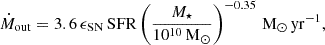
with ϵSN an efficiency parameter that we use to calibrate the mass loading factor; ϵSN = 1 corresponds to the results from Muratov et al. (2015, FIRE simulations, Hopkins et al. 2014). Note that ϵSN = 1 yields a loading factor consistent with what Herrera-Camus et al. (2021) observes for HZ4 (but see Parlanti et al. 2025). Further, using ϵSN = 1 in Eq. (2) would match the results from Pizzati et al. (2023) for z ≃ 5 − 6 ALPINE galaxies (Le Fèvre et al. 2020) that feature a spatially extended gas component (Fujimoto et al. 2020). However, ϵSN ≃ 1/3 is needed to match the loading factor inferred from z ≃ 3 − 9 JADES galaxies (Carniani et al. 2024). We note that simulated outflow loading factors (Muratov et al. 2015) are typically computed in a different way than is inferred from observations (e.g. Pizzati et al. 2020; Carniani et al. 2024). Thus, some care should be taken in the comparison, and our conclusions should be taken with caution as they are based on simplified assumptions. We assumed that the SFR is proportional to the gas mass:
 (2b)
(2b)
and we selected a constant t⋆ = 1 Gyr as our fiducial star formation timescale6. The choice of t⋆ is roughly consistent with the upper limits of the depletion times reported by Dessauges-Zavadsky et al. (2020) for ALPINE galaxies, and is discussed in more detail in Sect. 4.2 (see also Appendix A). To complete the model, we assumed that halos can form stars after they reach a virial temperature for atomic cooling to be effective (104 K); similarly to SERRA, we assumed return fraction and yields appropriate for a Kroupa (2001) IMF and adopting Bertelli et al. (1994) tracks with a Z⋆ = Z⊙ stellar population7, which gives y ≃ 0.0228 and R ≃ 0.3242. The system (Eqs. (1) and (2)) was solved along with z = z(t) using an embedded Runge-Kutta method (Fehlberg 1968) of order fifth(sixth) with an adaptive timestep, which was selected in order to have a fractional (absolute) precision of at least ≤10−5 (≤ 102 M⊙) for Mdm, M⋆, Mg, and  . The delayed SFR and stellar mass used to evaluate the stellar feedback were computed using a seven-point time stencil.
3.2. Overview of the minimal physical model
The delay between the SFR and feedback td and the amplitude of the outflow (ϵSN) regulate the burstiness of the galaxy in our single zone model (cf. Furlanetto & Mirocha 2022). To understand the impact of burstiness on galaxy evolution, it is instructive to consider a halo with mass Mdm = 3 × 10¹⁰ M⊙ at z = 6 and set the outflow efficiency to the standard value of ϵSN = 1. In Fig. 2 we compare the evolution of the stellar (green), gas (brown), and metal (pink) mass content for td = 0 (no-SN-delay, dashed lines) and td = 10 Myr (solid lines). By construction, the halo mass growth (Eq. (1a)) is unaffected by td, and thus the two models follow the same DM evolution (black line), which smoothly grows from Mdm ≃ 107 M⊙ at z ≃ 18, when the Universe was t ≃ 200 Myr old. At that time, for td = 0 the gas and stars has ≃105 M⊙ and ≃102 M⊙, respectively, and both grow, reaching approximately ≃5 × 10⁷ M⊙ at t ≃ 800 Myr, with M⋆/Mdm ≃ 5 × 10⁻³ broadly consistent with what is expected from abundance matching models (e.g. Behroozi et al. 2013). In the case with td = 10 Myr, the secular trends are qualitatively similar, but the system experiences a series of bursts on timescales of ≃20 Myr = 2 td. Let us focus on a single burst cycle around z ≃ 10, when the halo has Mdm≃ 109 M⊙ and M⋆ ≃ 106 M⊙. In the first half period of the cycle (0 − td), cosmic accretion quickly replenishes the gas (the gas infall rate is ≃ 0.5 M⊙ yr−1 from Eq. (1a)), reaching Mg ≃ 107 M⊙ in a few million years. Stars form at a modest rate, SFR ≃ 10−2 M⊙ yr−1 (Eq. (2b)), under feedback-free conditions (cf. Dekel et al. 2023). After td, the feedback kicks in, first enriching the galaxy and eventually (≃2 td) becoming powerful enough to expel both gas (gas outflow is ≃ 1 M⊙ yr−1 using Eq. (2a)) and metals (cf. Ferrara et al. 2023). Note that the delay effectively produces a sequence of mini-quenching periods (cf. Looser et al. 2024), which are commonly inferred in faint galaxies (Endsley et al. 2024) and which can be explained as a consequence of internal feedback (Gelli et al. 2025). However, in our minimal model, outflows are the only mechanism regulating the star formation, and quenching due to gas complete depletion, which might be too extreme a description of the actual physical evolution (but see Gelli et al. 2024b). Further, in the example, the impact of SFR flickering is limited already after z ≃ 15, when the galaxy has M⋆ ≃ 105 M⊙ or 10× lower if no delay is considered. At z ≃ 6, the final stellar mass is M⋆ ≃ 107 M⊙ within a factor of 2 for the two models. For the gas and metals, the model with SN-delay starts to converge to the no-SN-delay case at z ≃ 8, when M⋆ ≃ 107 M⊙; oscillations for the gas and metals are still present up to z ≃ 7, but they are milder. As in Pallottini & Ferrara (2023), it is convenient to quantify the burstiness of the SFR by defining the variable, δ, expressing the log of the stochastic SFR variation with respect to its mean (in short: flickering),
 |
Fig. 2. Example of the impact of SFR burstiness on the evolution of a galaxy hosted in a Mdm = 3 × 10¹⁰ M⊙ DM halo at z = 6 using the minimal physical model described in Sect. 3.1 (see in particular Eqs. (1)). The time evolution of the DM (black), star (green), gas (brown), and metal (pink) mass (M) content is shown with solid (dashed) lines for a SN-delay time of td = 10 Myr (td = 0, i.e. no delay). The upper axis shows the redshift, z, corresponding to cosmic time, t. |
 (3a)
(3a)
where  is a second-order polynomial fit in the time variable, t. The low-order fit is needed to factor out the smooth behavior of the functions without removing time modulations (see Leja et al. 2019; Chaves-Montero & Hearin 2021, for alternative methods). As in Pallottini & Ferrara (2023), we used a 2 Myr timescale binning when evaluating SFR in Eq. (3), while no explicit time averaging was needed for ⟨SFR⟩, since it was implicitly done via the polynomial fit (cf. Sun et al. 2023a). Similarly to the flickering, we defined the analog variable for the gas metallicity,
 (3b)
(3b)
where log⟨Zg/Z⊙⟩ is a second-order polynomial fit in the variable log M⋆/M⊙. For both δ and δZ, we can define the typical variation as the rms deviation, i.e., σSFR and σZ, respectively. Adopting Eqs. (3), we find that the td = 10 Myr case has a flickering of σSFR ≃ 0.3 before the two models start to converge, which is slightly higher than the σSFR ≃ 0.24 obtained for SERRA galaxies (Pallottini & Ferrara 2023). For different td the qualitative behavior is very similar, as the model is off-balance and oscillates around the no-SN-delay case, which is similar to a bathtub solution (Bouché et al. 2010; Dekel & Mandelker 2014). For shorter (longer) td, σSFR can be smaller (higher), as a galaxy with a smaller (higher) M⋆ can be off-balanced. The balance between infall and outflow rates is critical, since the dynamical system (Eqs. (1)) modeling the galaxy evolution gives rise to exponentially increasing or decreasing trends; introducing a td ≠ 0 can efficiently break the balance, causing cycles of complete gas and metal depletion. To explore the MZR variations induced by the flickering, in Fig. 3 we plot the tracks of the selected Mdm = 3 × 10¹⁰ M⊙ at z = 6 with td from 5 to 25 Myr. Because of the longer td, the SFR becomes increasingly bursty. Specifically, for the selected model the flickering ranges from σSFR ≃ 0.1 to σSFR ≃ 0.6 for td = 5 Myr to td = 25 Myr, respectively. The MZR modulations induced by the flickering are highly nonlinear. With td = 5 − 10 Myr, the MZR dispersion is small (σZ ≃ 0.05 − 0.2), as the flickering can affect galaxies only up to M⋆≃ 105−7 M⊙. For td = 15 Myr, the full M⋆ range experiences flickering with a σSFR ≃ 0.5, yielding a high σZ ≃ 0.8. Cases with td > 15 Myr do not show a higher stochasticity, as an increasing delay only regulates which M⋆ can be affected by the feedback unbalance8. Qualitatively, the behavior is similar to higher Mdm, but the convergence to the bathtub solution is faster. For the effect of a coarse time sampling, see Appendix B (in particular Fig. B.1). In summary, a feedback delay induces a stochastic, bursty star formation behavior that becomes progressively more enhanced as td is increased. Such SFR flickering corresponds to analog Zg fluctuations, which act to decrease the mean metallicity as gas and metals are effectively ejected from the galaxy by outflows.
 |
Fig. 3. Example of the impact of SFR burstiness on the MZR for a system with Mdm = 3 × 10¹⁰ M⊙ at z = 6 evolved with our minimal physical model. Different lines indicate different delay times for the SN feedback, as is indicated in the legend. Note that the model results have been resampled in 0.2 Myr steps and we do not consider the evolutionary phases when the galaxies have a negligible amount of gas (Mg ≤ 10−3 Mdm), which allows us to have a well-defined Zg even in periods when no gas and metals are present in the galaxy (see Fig. 2). For the effect of a coarser time sampling, see Appendix B, in particular Fig. B.1. |
3.3. The impact of a stochastic SFR on the MZR
We ran sets of models that at z = 6 have a Mdm from 109 M⊙ to 1013 M⊙ with a logarithmic binning of 0.1 dex, in order to cover the mass range 105 M⊙≲ M⋆ ≲ 5 × 10¹⁰ M⊙. We analyzed different variations of the minimal models, reporting the results in different panels of Fig. 4, where they were compared with data from JWST observations (Nakajima et al. 2023; Curti et al. 2024; Chemerynska et al. 2024b).
 |
Fig. 4. Predicted MZR relation for different sets of minimal models with 109 M⊙ ≤ Mdm ≤ 1013 M⊙ halos at z = 6. In the upper left panel, we report the “base models” with ϵSN and td = 20 Myr (see Sect. 3.2). In the upper right panel, we modify the base model by reducing the efficiency of the feedback (ϵSN = 1/4 in Eq. (2a)). In the lower left panel, we consider both weak feedback and a cosmic accretion that is modulated on a timescale of 100 Myr (A100 = 1/3 in Eq. (4)). In the lower left panel, we show the effect of turning off the SN-delay for the weak feedback models with modulated cosmic accretion. In each panel, pastel lines are the individual tracks sampled every 2 Myr; their median and 16 − 84% dispersion are plotted with dashed and solid violet lines, respectively; the dashed black line is the control case with no-SN-delay (td = 0) and no modulated accretion (A100 = 0). For each model, we report the value values of the SFR flickering (σSFR) and the MZR dispersion (σZ, see Fig. 5). As in Fig. 1, we show JWST data and fits (Nakajima et al. 2023; Curti et al. 2024; Chemerynska et al. 2024b). |
3.3.1. Base models
Let us start by discussing the “base models‘’ analyzed in Sect. 3, i.e., with ϵSN = 1, consistent with FIRE simulations (Muratov et al. 2015), and selecting td = 20 Myr, so that most of the explored stellar mass range is expected to have a stochastic SFR. In the upper left panel of Fig. 4 we report both the individual tracks of the base models and their M⋆ average trends. For the base models, the median case falls significantly below the observed average MZR. Also, the dispersion is much larger than what is seen in JWST data, which can be barely matched by the upper envelope of the predicted curves. The base models have a σSFR ≃ 0.5 flickering, which induces a σZ ≳ 1 almost in the entire stellar mass range (M⋆ ≲ 109 M⊙, Fig. 5). The flickering is due to cycles of infall and outflow that determine an oscillatory behavior of the evolution around the td = 0 control case, which is largely independent of the hosting Mdm. The Zg–M⋆ normalization is determined by the strength of the outflows, which makes the galaxy completely devoid of gas and metals, preventing the metallicity from rising to the observed level. Even for td = 0 the outflow seems too extreme, as only part of the lensed galaxy data can be matched (Chemerynska et al. 2024b). In summary, the efficient feedback (ϵSN = 1) combined with a td = 20 Myr generates a SFR flickering of σSFR ≃ 0.5, inducing MZR variations of σZ ≃ 1.4 resulting in a “chemical chaos” that is not observed. Barring the option that observations are tracing only the tip of the Zg–M⋆ relation, in order to explain the observed MZR we modified the base models as follows.
3.3.2. Weak feedback
First, we reduced the impact of stellar feedback by decreasing the outflow rate from Muratov et al. (2015) (Eq. (2a)), i.e., setting ϵSN = 1/4; such a loading factor is closer to what Carniani et al. (2024) infer for 107.5 ≲ M⋆ ≲ 109 M⊙ JADES galaxies. As is shown in the upper right panel of Fig. 4, this modification increases the average metallicity of the modeled galaxies, matching the observed mean trends in the whole 106 M⊙≲ M⋆ ≲ 1010 M⊙ mass range. Compared to the td = 0 control case, it is evident that the outflow efficiency is the main driver of the mean Zg–M⋆ trend. Note that reducing the outflow efficiency while maintaining a fixed td = 20 Myr results in σZ ≃ 0.1 modulation of the MZR, i.e., too low with respect to the observed (σZ ≃ 0.25, see Fig. 5). This effect is induced by the suppression of the amplitude of the SFR flickering, especially at the high-mass end. Indeed the models show a small flickering, with σSFR ≃ 0.15 for M⋆ ≲ 108 M⊙, and even slightly lower values for higher stellar masses (Fig. 5). As is discussed in Pallottini & Ferrara (2023), M⋆ ≲ 109 M⊙ galaxies show SFR fluctuations with characteristic periods of ≃20 − 40 Myr, which correspond to the typical evolutionary times of SNe. Such a flickering timescale increases to ≃80 − 150 Myr in more massive galaxies, which are more sensitive to mergers and accretion rate modulation. The latter effects are not accounted for in our minimal model (Eq. (1a)). The next step was then to heuristically incorporate them into our treatment.
3.3.3. Weak feedback, modulated accretion
To incorporate the extra stochastic behavior expected from variation in the cosmic accretion and merger in a simple manner, we imposed a sinusoidal modulation on a 100 Myr timescale,
![Mathematical equation: $$ \begin{aligned} \dot{M}_{dm}^{mod}= \dot{M}_{dm} \left[1 + A_{100}\sin \left(\frac{2 \pi t }{100 \,\mathrm{Myr}}\right)\right], \end{aligned} $$](/articles/aa/full_html/2025/07/aa51742-24/aa51742-24-eq13.gif) (4)
(4)
with Ṁdm being the average cosmic accretion from Eq. (1a) and with A100 scaling the amplitude of the modulation9. For different galaxies, a phase shift is implicitly included because star formation starts when the hosting halo mass is larger than the atomic cooling halo threshold. While our inclusion of the accretion modulation is effective, it is very crude (for a more refined treatment, see Sun et al. 2025, which adopts a modulation based on random extractions of variation in the accretion histories by using a predefined power spectral density). As feedback determines the mean trend of the MZR, we kept the reduced outflow efficiency (ϵSN = 1/4 in Eq. (2a)) and computed the evolution of a minimal model by setting the amplitude of the oscillation to A100 = 1/3, which should yield a scatter below the 0.3 dex dispersion expected for the distribution of growth rates of DM halos (Rodríguez-Puebla et al. 2016; Ren et al. 2019; Mirocha et al. 2021). The results from these modified models are shown in the lower left panel of Fig. 4: both the mean trend and scatter of the observed MZR are recovered (Fig. 5). Such a matching set of modified models yields a roughly constant σSFR ≃ 0.2 and σZ ≃ 0.3, satisfactorily matching the JWST data.
3.3.4. Weak feedback, modulated accretion, no-SN-delay
As a final check, in the lower right panel of Fig. 4 we show the effect of removing the SN-delay from the best-matching model just discussed. While the mean MZR trend is recovered, the metallicity dispersion (σZ ≃ 0.05) is much smaller than observed (σZ ≃ 0.25). Also, the median of the models fails to reproduce the relation for most of the low-mass lensed galaxies (Chemerynska et al. 2024b). In the no-SN-delay case, the SFR flickering is induced only by modulation of the cosmic accretion, which fails to unbalance the system through the ejection of a substantial fraction of the contained gas. With the selected A100 = 1/3 and td = 0, the model reaches σSFR ≃ 0.1 for M⋆ ≲ 108 M⊙, while the flickering gets to σSFR ≃ 0.2 only for M⋆≃ 5 × 10⁸ M⊙ galaxies. Compared to the control case (A100 = 0), the average Zg is slightly higher; practically, SFR flickering induced by the accretion modulation can increase Zg since a higher gas mass can be converted into stars without efficiently ejecting the gas via outflows, i.e., the opposite outcome with respect to SFR flickering induced via SN-delay. Interestingly, despite the relatively high SFR flickering (average of σSFR ≃ 0.2), the metallicity variation is the lowest of all the considered cases (σZ ≃ 0.05): only a delayed SN feedback can efficiently off-balance the system and induce modulations on both SFR and Zg. We note that the SERRA cosmological simulations show a relatively modest SFR flickering (σSFR ≃ 0.24, Pallottini & Ferrara 2023), and are close to the expectations for z ≃ 6 galaxies (Muñoz et al. 2023; Ciesla et al. 2024). Yet, given the sharp sensitivity of σZ to SFR variations, such time variability results in a σZ larger than what is observed. To summarize, our analysis shows that: (i) weak feedback, and (ii) relatively mild stochasticity given by (iii) SN-delay combined with a long-term accretion rate modulation are critical to simultaneously match both the mean and dispersion of the observed MZR relation in the entire stellar mass range of galaxies sampled by JWST at z = 3 − 10. Interestingly, we note that invoking stochasticity to explain the overabundance of bright JWST galaxies requires σSFR > 0.5 (more specifically, σSFR ≃ 0.8, σSFR ≃ 0.7, and σSFR ≃ 0.6 according to Muñoz et al. 2023; Shen et al. 2023, and Mason et al. 2023, respectively; see Fig. 5). However, such extreme flickering amplitudes are (i) higher than that recovered from SED fitting allowing for SFH variability (σSFR ≲ 0.5, Ciesla et al. 2024), and (ii) would induce a chemical chaos (σZ ≳ 1.4) that is not present in the observed MZR at z = 3 − 10 (σZ ≃ 0.25 from Nakajima et al. 2023; Curti et al. 2024; Chemerynska et al. 2024b data, σZ ∼ 0.3 reported by Heintz et al. 2023; Morishita et al. 2024). Indeed, adopting the FIRE-2 model, Sun et al. (2023a) report that the overabundance of bright super-early galaxies can be matched; Marszewski et al. (2024) find a MZR dispersion at M⋆≲ 108.5 M⊙ that is roughly twice the average σZ observed by JWST. The drop in σZ from FIRE-2 at M⋆ ≳ 108.5 M⊙ might be caused by the low number of galaxies in that mass bin (see Fig. 1 from Marszewski et al. 2024) or a reduction in the flickering at higher stellar masses (compare with Fig. 13 from Kravtsov & Belokurov 2024). Finally, note that Katz et al. (2024) reports that galaxies dominated by a strong nebular continuum (Balmer jump galaxies) can have UV flux increases that might help to reconcile the surprising abundance of bright high-z galaxies; however, the incidence of Balmer jump galaxies is unconstrained at z ≳ 10 and the magnitude of the effect is relatively small (≃0.28 dex in terms of σSFR). Even if all the systems were Balmer jump galaxies, high flickering (or a different mechanism) would still need to be invoked to explain the overabundance of bright super-early galaxies.
4. Discussion
The minimal models presented here can also be useful as a tool to guide the development and compare complex cosmological simulations, particularly when focusing on relations that – like the MZR – are very sensitive to small variations in the underlying physics, which is included via sub-grid models in galaxy simulations (Agertz et al. 2020).
4.1. Comparing numerical simulations
In galaxy simulations, ejective feedback, such as outflows caused by mechanical or kinetic prescriptions, can effectively suppress the SFR activity as much as preventative feedback, such as turbulence or delayed cooling prescriptions (Rosdahl et al. 2017), leading to similar SFR histories when the same initial conditions are considered (Lupi et al. 2020). Despite similar SFR histories, other properties can differ significantly (Rosdahl et al. 2017), such as the dynamical state of a galaxy. In the minimal model, ϵSN regulates the level of SFR suppression and determines the MZR normalization. In simulations, the level of SFR suppression can be quantified by the M⋆ − Mh relation. FIRE-2 predicts a M⋆ − Mh similar to Behroozi et al. (2013); SERRA is also consistent with Behroozi et al. (2013) for M_h ≳ 1011 M⊙ (M⋆ ≳ 109 M⊙), but on average10 tends to be above such a relation for M_h≲ 109 M⊙. Indeed, SERRA and FIRE-2 give the same normalization for the MZR (see Fig. 1) in the stellar mass range where the M⋆ − Mh is similar, while for 107 ≲ M⋆/M⊙ ≲ 109 SERRA predicts a higher MZR normalization. In the minimal model, the SFR flickering is regulated by td, which determines the MZR scattering. In simulations, the SFR flickering is regulated by the adopted feedback type (ejective vs. preventative). The MZR scatter is similar in SERRA and FIRE-2 (Marszewski et al. 2024) only for M⋆ ≳ 109 M⊙ (see Fig. 5). This is not surprising, as a higher SFR flickering is reported in FIRE-2 (Sun et al. 2023b) with respect to SERRA (Pallottini & Ferrara 2023), which can have further consequences on top of UV variations. Higher SFR flickering in FIRE-2 is due to violent outflows (Hopkins et al. 2018), while the suppression of SFR due to the photo-dissociation of molecular hydrogen in SERRA (Pallottini et al. 2019) can more gently modulate the SFR activity without drastically modifying the galaxy dynamics. Indeed, Fujimoto et al. (2024) show that FIRE-2 galaxies (Wetzel et al. 2023) have a much lower incidence of disks compared to SERRA galaxies (Kohandel et al. 2024) at M⋆ ≳ 5 × 10⁸ M⊙, i.e., although the SFR regulation in the two simulations is similar. Despite the simplicity of the minimal model presented, hints of such differences in the simulations can be highlighted and explained. However, it is difficult to directly quantify the differences in the simulations with the presented models. For instance, the loading factor in our simplified models (but also in more complex ones such as those of Thompson et al. 2016 and Pizzati et al. 2020) is a scalar quantity used as an input value for each galaxy, while in simulations it is usually defined as an output that has a spatial dependence (Gallerani et al. 2018). Additionally, a precise quantification can be difficult. For instance, the MZR from FIRE-2 (Marszewski et al. 2024) is about 0.3 dex higher than the MZR from FIRE (Ma et al. 2016); in both cases, the slope is steeper (normalization is lower) than what is observed by Nakajima et al. (2023), Curti et al. (2024) and is instead more consistent with Chemerynska et al. (2024b). However, the two simulations have the same loading factor (Pandya et al. 2021), and thus it is difficult to explain the difference only in terms of our minimal models. Moreover, when dealing with simulation snapshots, quantifying both the SFR event and the consequent outflows is tricky because of the time delay between SFR and feedback (Pandya et al. 2021), particularly for galaxies far from a quasi-equilibrium situation. Furthermore, the simplifications done in our minimal model impose that we can only capture part of the complexity present in simulations. For instance, while the SN feedback delay is uniquely defined, simulations find a distribution of td that depends on the underlying physical models included (Pallottini & Ferrara 2023); thus, trying to find the set of parameters of a minimal model that gives the best match to a simulation will only give “effective” parameters, a sort of summary statistic that can be used to compare different simulations. Apart from these difficulties, a systematic parameter fitting procedure should give a better quantification of the comparison between different simulations, and can also be used to enable an even better match between the data and the minimal models. However, such models lack a few ingredients that prevent them from reproducing the full connection between metal buildup and the SFH of galaxies.
4.2. Caveats of the minimal model
The limitations of the presented minimal models can be appreciated by considering the FMR, i.e., the link between Zg, M⋆, and SFR that is observed to be redshift-independent up to z ∼ 3 (Mannucci et al. 2010; Curti et al. 2020) and seems to break down at z ≳ 5 (Nakajima et al. 2023; Curti et al. 2024). We adopted the parameterization from Curti et al. (2020),
 (5)
(5)
which was obtained by minimizing the Zg dispersion for the high sSFR subsample from the Sloan Digital Sky Survey (SDSS, York et al. 2000, z ≲ 2). In Fig. 6 we show the FMR for the minimal models matching the mean MZR and its dispersion, i.e., the weak feedback (ϵSN = 1/4) set with modulated accretion (A100 = 1/3). These models are below the SDSS relation by about 0.5 dex at μ ≲ 7, with the separation that decreases with increasing μ, down to 0.1 dex at μ ≳ 9, almost connecting with the FMR trend observed at low z. As was expected (Nakajima et al. 2023; Curti et al. 2024), JWST galaxies are offset below the SDSS relation. The best matching models for the MZR only partially match the JWST data in the FMR plane; the minimal models are closer to the JWST data when considering the lensed galaxies from Chemerynska et al. (2024b). Further, the minimal models only produce downward deviation with respect to the FMR from the SDSS. Instead, SERRA galaxies manage to better recover the trend for JWST galaxies around μ ≃ 8, reproducing both downward and upward deviations with respect to the FMR from the SDSS; however, SERRA galaxies show an overabundance of low Zg galaxies at μ ≃ 8.5 − 9.0, which is not seen in the JWST data. In an equilibrium model (Lilly et al. 2013), the shape of the MZR is independent of the SFR, which uniquely determines the speed at which a galaxy can climb up the Zg–M⋆ curve. Note that the simplified model seems to deviate more from the data at low μ, i.e., a combination of relatively high SFR and low M⋆; the adopted feedback increases in efficiency for lower M⋆ (Eq. (2a)). Thus, the observed FMR deviation might be recovered by the minimal model if we consider not only ejecting but also preventing feedback, such as photo-dissociation of molecular hydrogen, which can suppress the star formation without affecting the gas mass (e.g., see Alyssum, a SERRA galaxy described in Pallottini et al. 2022) and can play a role in explaining some of the bright blue monsters seen by JWST (Ferrara 2024). As an alternative to keep matching the MZR and recovering the offset from the FMR, we could try to change the simplified SFR prescription (Eq. (2b)); this can be done, for instance, by adopting as the timescale for star formation a redshift-dependent depletion time (Tacconi et al. 2010, 2020; Sommovigo et al. 2022), which is typically shorter than the selected t⋆ = 1 Gyr by about a factor ≃10, similar to what Vallini et al. (2024) report for z ≃ 7 galaxies by using GLAM (Vallini et al. 2020, 2021) determinations, and thus promoting a faster galaxy evolution at high-z. Indeed, by adopting the depletion time from Sommovigo et al. (2022) as the timescale for SFR (see Appendix A, in particular, Fig. A.1), the stellar mass buildup is faster at M⋆ ≲ 106 M⊙, while it later saturates to values similar to those resulting from the t⋆ = 1 Gyr case as both SFHs become feedback-regulated, approaching a bathtub equilibrium. On the one hand, the modifications affect the predictions of the minimal model mostly in the M⋆ ≲ 106 M⊙ range; on the other hand, a z average depletion time is sensitive to the population of the sample – for example, for the main sequence it is ≃ × 5 lower than for starbursts (Tacconi et al. 2020) – and the results from Sommovigo et al. (2022) rely mostly on the data of M⋆ ≳ 108−10 M⊙ galaxies from the ALPINE (Le Fèvre et al. 2020) and REBELS (Bouwens et al. 2022) surveys. To summarize, while trying to reconcile the FMR behavior is an interesting perspective and there are a few options, some care should be taken in extending and/or modifying the prescriptions for the minimal models; we leave such a possibility for future work.
 |
Fig. 6. Deviation from the FMR for high-z galaxies. We adopt the |

5. Conclusions
The exquisite spectroscopic data collected by JWST allow us for the first time to derive the MZR in galaxies up to redshift z ≃ 10. In this work, we have considered the MZR data for a combined sample of about 180 galaxies with a stellar mass of 106 M⊙≲ M⋆ ≲ 1010 M⊙ at z = 3 − 10 given by Nakajima et al. (2023), Curti et al. (2024), and Chemerynska et al. (2024b), and obtained from the CEERS (Finkelstein et al. 2023), JADES (Bunker et al. 2024), and UNCOVER (Bezanson et al. 2024) surveys, respectively. We compared the observations with the predictions from the SERRA simulations (Pallottini et al. 2022), finding a broad agreement with the observed Zg − M⋆ data. However, the simulations show a lack of a clear metallicity trend (flat MZR), and some tension, particularly at M⋆≃ 1010 M⊙. To better understand the observed high-z MZR and to clarify the behavior of the simulations, we have devised a minimal physical model for galaxy evolution in which star formation is fueled by cosmic gas accretion (Correa et al. 2015) and regulated by SN-driven outflows (Eq. (2a)), with a loading factor from Muratov et al. (2015) that is controlled by an efficiency, ϵSN. Additionally, we incorporated an explicit delay (td) between star formation and supernova feedback, inducing a stochastic SFR behavior. Some models also explore the possible modulation of cosmic accretion (Eq. (4)). The main results are:
-
To recover the average trend of the MZR observed at high-z, outflows must be less efficient (ϵSN = 1/4) than what was predicted in Muratov et al. (2015). However, this evidence is consistent with the mass loading factors inferred for JADES galaxies (Carniani et al. 2024).
-
To match the MZR dispersion in the full stellar mass range, both delayed (td = 20 Myr) SN feedback and modulation of the cosmic accretion (A100 = 1/3) are required.
-
The rms variation of the MZR (σZ) is very sensitive to the SFR flickering (σSFR). The weak feedback necessary to reproduce the average MZR trend (ϵSN = 1/4) also results in low-amplitude SFR flickering (σSFR ≃ 0.2). This prescription correctly reproduces the moderate MZR scatter (σZ ≃ 0.25) observed by JWST.
-
SERRA galaxies have slightly higher σSFR ≃ 0.24 (Pallottini & Ferrara 2023), resulting in a metallicity scatter of σZ ≃ 0.3, higher than what is observed. Unlike the analytical model, SERRA galaxies also overpredict the number of low-metallicity (Zg ≃ 0.2 Z⊙) galaxies at M⋆≃ 1010 M⊙.
-
In general, any model predicting σSFR ≳ 0.5 is likely to overshoot the observed metallicity rms scatter, possibly leading to a “chemical chaos” (σZ ≳ 1.4) that is not present in JWST data, for which σZ ≃ 0.25.
The last point also entails that simultaneously explaining the observed MZR (Nakajima et al. 2023; Curti et al. 2024) and the overabundance of bright galaxies observed by JWST (Finkelstein et al. 2022; Naidu et al. 2022) through high SFR flickering (Mason et al. 2023; Mirocha & Furlanetto 2023; Shen et al. 2023; Sun et al. 2023a; Kravtsov & Belokurov 2024) is very challenging, considering that a σSFR ≃ 0.8 is required to explain z > 10 observations (Muñoz et al. 2023). We note that while both the SN-feedback delay and cosmic accretion modulation induce SFR flickering, the latter tends to give a gentler modulation of Zg, since high feedback efficiency and a delay are needed in order to off-balance the MZR generated from a bathtub-like equilibrium (Lilly et al. 2013). However, variation in cosmic accretion can only go up to 0.3 dex (Rodríguez-Puebla et al. 2016; Ren et al. 2019; Mirocha et al. 2021). Thus, alternative explanations (Dekel et al. 2023; Ferrara et al. 2023) seem more likely to solve the overabundance problem. As was noted in the introduction1, we caution that we are taking the observed MZR scattering at face value, while this quantity might be affected in a nontrivial way by uncertainties in the Zg determinations. However, observationally the MZR has been explored by different groups, samples, and methods, i.e., metallicity determinations are available with both auroral lines that can be used to directly compute the electron temperature (Morishita et al. 2024) and indirect methods based on combinations of various calibrators (Heintz et al. 2023; Nakajima et al. 2023; Curti et al. 2024). It is reassuring to see that these works and datasets independently report a similar scattering of ≃0.3 − 0.5 dex. For this reason, we consider the current measurements of the MZR dispersion to be relatively robust. In the future, it is likely that the dispersion might decrease, given that the current sample size is relatively small (∼200 galaxies) and covers a relatively large redshift range (z ≃ 3 − 10). While we showed that the presented minimal model can also be used to guide our intuition in comparing complex cosmological simulations, we recall that such a simplified model does not fully capture the physical complexity of the connection between galaxy formation and metal enrichment, as is highlighted by the poor match with the JWST data when analyzing the offset from the FMR. Combining insights from such models with further analysis of ongoing observations, and more complex numerical simulations, is crucial for understanding the galaxy formation and evolution process at high-z.
As far as we are aware, specific studies of the intrinsic scatter of the MZR relation are not present for JWST targets (cf. with Strom et al. 2022, for z = 2 − 3 scattering determinations), thus we take the observed scattering at face value.
We adopt a ΛCDM model with vacuum, matter, and baryon densities in units of the critical density ΩΛ = 0.692, Ωm = 0.308, Ωb = 0.0481, normalized Hubble constant h = H0/(100 km s−1 Mpc−1) = 0.678, spectral index n = 0.967, and σ8 = 0.826 (Planck Collaboration XVI 2014).
Different assumptions on the integration radius produce only small changes in the inferred metallicity.
We have checked the SERRA data at z = 7, 8, and 9.
While FIRE-2 adopts Z⊙ = 0.02 as SERRA, the former simulation also track O abundance; Marszewski et al. (2024) finds [O/H]⊙ + 12 = 9.0 for FIRE-2 instead of the [O/H]⊙ + 12 = 8.69 (Asplund et al. 2009) adopted here for the conversion of the observations. Adopting the [O/H]⊙ + 12 = 9.0 conversion for FIRE-2 would make the agreement with observations better in the low-mass regime, leaving unaltered the slope, scatter, and relative considerations.
In the model, galaxy evolution is self-regulated by feedback, thus the sensitivity of the results from t⋆ is limited in our case, and null in the td = 0 case with constant loading factors for infall and outflow (Lilly et al. 2013). A posteriori, we note that the fiducial t⋆ = 1 Gyr gives specific star formation rates, sSFR = SFR/M⋆, which are consistent with SERRA galaxies, i.e. ≃sSFR ≃ 100 − 1 Gyr−1 for galaxies with masses M⋆ = 106−1010 M⊙.
Changing the metallicity of the stellar population does modifies the yield and return fraction, but gives only minor modifications to the upcoming results.
Note that a higher/lower level of flickering can be induced by changing the infall/outflow rates, as shown later in Sect. 3.3.
Note that small halos should be less affected by modulation on long timescales (≃100 Myr), since the hosted galaxies have shorter SFHs. However, cosmological accretion variations can be coherently combined with the SN-delay to also give a higher σSFR in the low-mass range.
When M⋆ ≲ 106 M⊙, SERRA galaxies can be temporarily below the M⋆ − Mh relation from Behroozi et al. (2013) because of high radiation field and low dust content, which cause an efficient H2 photo-dissociation, see the Alyssum effect in Pallottini et al. (2022).
Acknowledgments
We acknowledge the CINECA award under the ISCRA initiative, for the availability of high-performance computing resources and support from the Class B project SERRA HP10BPUZ8F (PI: Pallottini). AF acknowledges support from the ERC Advanced Grant INTERSTELLAR H2020/740120 (PI: Ferrara). SC and GV acknowledge support support from the ERC Starting Grant WINGS H2020/101040227 (PI: Carniani). Any dissemination of results must indicate that it reflects only the author’s view and that the Commission is not responsible for any use that may be made of the information it contains. Partial support (AF) from the Carl Friedrich von Siemens-Forschungspreis der Alexander von Humboldt-Stiftung Research Award is kindly acknowledged. We gratefully acknowledge the computational resources of the Center for High Performance Computing (CHPC) at SNS. We acknowledge usage of the Python programming language (Van Rossum & de Boer 1991; Van Rossum & Drake 2009), Astropy (Astropy Collaboration 2013), Cython (Behnel et al. 2011), Matplotlib (Hunter 2007), Numba (Lam et al. 2015), NumPy (van der Walt et al. 2011), PYNBODY (Pontzen et al. 2013), and SciPy (Virtanen et al. 2020).
References
- Adams, N. J., Conselice, C. J., Ferreira, L., et al. 2023, MNRAS, 518, 4755 [Google Scholar]
- Agertz, O., Pontzen, A., Read, J. I., et al. 2020, MNRAS, 491, 1656 [Google Scholar]
- Andrews, B. H., & Martini, P. 2013, ApJ, 765, 140 [NASA ADS] [CrossRef] [Google Scholar]
- Asplund, M., Grevesse, N., Sauval, A. J., & Scott, P. 2009, ARA&A, 47, 481 [NASA ADS] [CrossRef] [Google Scholar]
- Astropy Collaboration (Robitaille, T. P., et al.) 2013, A&A, 558, A33 [NASA ADS] [CrossRef] [EDP Sciences] [Google Scholar]
- Atek, H., Shuntov, M., Furtak, L. J., et al. 2023, MNRAS, 519, 1201 [Google Scholar]
- Behnel, S., Bradshaw, R., Citro, C., et al. 2011, Comput. Sci. Eng., 13, 31 [Google Scholar]
- Behroozi, P. S., Wechsler, R. H., & Conroy, C. 2013, ApJ, 770, 57 [NASA ADS] [CrossRef] [Google Scholar]
- Bertelli, G., Bressan, A., Chiosi, C., Fagotto, F., & Nasi, E. 1994, A&AS, 106, 275 [NASA ADS] [Google Scholar]
- Bezanson, R., Labbe, I., Whitaker, K. E., et al. 2024, ApJ, 974, 92 [NASA ADS] [CrossRef] [Google Scholar]
- Bothwell, M. S., Maiolino, R., Kennicutt, R., et al. 2013, MNRAS, 433, 1425 [Google Scholar]
- Bouché, N., Dekel, A., Genzel, R., et al. 2010, ApJ, 718, 1001 [Google Scholar]
- Bouwens, R. J., Smit, R., Schouws, S., et al. 2022, ApJ, 931, 160 [NASA ADS] [CrossRef] [Google Scholar]
- Bunker, A. J., Cameron, A. J., Curtis-Lake, E., et al. 2024, A&A, 690, A288 [NASA ADS] [CrossRef] [EDP Sciences] [Google Scholar]
- Cameron, A. J., Katz, H., & Rey, M. P. 2023, MNRAS, 522, L89 [NASA ADS] [CrossRef] [Google Scholar]
- Carniani, S., Venturi, G., Parlanti, E., et al. 2024, A&A, 685, A99 [NASA ADS] [CrossRef] [EDP Sciences] [Google Scholar]
- Carniani, S., D’Eugenio, F., Ji, X., et al. 2025, A&A, 696, A87 [NASA ADS] [CrossRef] [EDP Sciences] [Google Scholar]
- Casavecchia, B., Maio, U., Péroux, C., & Ciardi, B. 2024, A&A, 689, A106 [NASA ADS] [CrossRef] [EDP Sciences] [Google Scholar]
- Castellano, M., Fontana, A., Treu, T., et al. 2022, ApJ, 938, L15 [NASA ADS] [CrossRef] [Google Scholar]
- Ceverino, D., Glover, S. C. O., & Klessen, R. S. 2017, MNRAS, 470, 2791 [NASA ADS] [CrossRef] [Google Scholar]
- Chaves-Montero, J., & Hearin, A. 2021, MNRAS, 506, 2373 [NASA ADS] [CrossRef] [Google Scholar]
- Chemerynska, I., Atek, H., Furtak, L. J., et al. 2024a, MNRAS, 531, 2615 [NASA ADS] [CrossRef] [Google Scholar]
- Chemerynska, I., Atek, H., Dayal, P., et al. 2024b, ApJ, 976, L15 [NASA ADS] [CrossRef] [Google Scholar]
- Ciesla, L., Elbaz, D., Ilbert, O., et al. 2024, A&A, 686, A128 [NASA ADS] [CrossRef] [EDP Sciences] [Google Scholar]
- Correa, C. A., Wyithe, J. S. B., Schaye, J., & Duffy, A. R. 2015, MNRAS, 450, 1521 [NASA ADS] [CrossRef] [Google Scholar]
- Cueto, E. R., Hutter, A., Dayal, P., et al. 2024, A&A, 686, A138 [NASA ADS] [CrossRef] [EDP Sciences] [Google Scholar]
- Curti, M., Cresci, G., Mannucci, F., et al. 2017, MNRAS, 465, 1384 [Google Scholar]
- Curti, M., Mannucci, F., Cresci, G., & Maiolino, R. 2020, MNRAS, 491, 944 [Google Scholar]
- Curti, M., Maiolino, R., Curtis-Lake, E., et al. 2024, A&A, 684, A75 [NASA ADS] [CrossRef] [EDP Sciences] [Google Scholar]
- Curti, M., Witstok, J., Jakobsen, P., et al. 2025, A&A, 697, A89 [Google Scholar]
- Davies, F. B., & Furlanetto, S. R. 2016, MNRAS, 460, 1328 [NASA ADS] [CrossRef] [Google Scholar]
- Dayal, P., & Ferrara, A. 2018, Phys. Rep., 780, 1 [Google Scholar]
- Dayal, P., Ferrara, A., & Dunlop, J. S. 2013, MNRAS, 430, 2891 [Google Scholar]
- Decataldo, D., Pallottini, A., Ferrara, A., Vallini, L., & Gallerani, S. 2019, MNRAS, 487, 3377 [Google Scholar]
- Dekel, A., & Mandelker, N. 2014, MNRAS, 444, 2071 [NASA ADS] [CrossRef] [Google Scholar]
- Dekel, A., Sarkar, K. C., Birnboim, Y., Mandelker, N., & Li, Z. 2023, MNRAS, 523, 3201 [NASA ADS] [CrossRef] [Google Scholar]
- Dessauges-Zavadsky, M., Ginolfi, M., Pozzi, F., et al. 2020, A&A, 643, A5 [NASA ADS] [CrossRef] [EDP Sciences] [Google Scholar]
- Dome, T., Tacchella, S., Fialkov, A., et al. 2024, MNRAS, 527, 2139 [Google Scholar]
- Donnan, C. T., McLeod, D. J., Dunlop, J. S., et al. 2023, MNRAS, 518, 6011 [Google Scholar]
- Ellison, S. L., Patton, D. R., Simard, L., & McConnachie, A. W. 2008, ApJ, 672, L107 [NASA ADS] [CrossRef] [Google Scholar]
- Endsley, R., Chisholm, J., Stark, D. P., Topping, M. W., & Whitler, L. 2024, ApJ, submitted [arXiv:2410.01905] [Google Scholar]
- Erb, D. K., Shapley, A. E., Pettini, M., et al. 2006, ApJ, 644, 813 [NASA ADS] [CrossRef] [Google Scholar]
- Fehlberg, E. 1968, Classical Fifth-, Sixth-, Seventh-, and Eighth-Order Runge-Kutta Formulas with Stepsize Control, NASA Technical Report [Google Scholar]
- Ferrara, A. 2008, in Low-Metallicity Star Formation: From the First Stars to Dwarf Galaxies, eds. L. K. Hunt, S. C. Madden, & R. Schneider, 255, 86 [Google Scholar]
- Ferrara, A. 2024, A&A, 689, A310 [NASA ADS] [CrossRef] [EDP Sciences] [Google Scholar]
- Ferrara, A., Pallottini, A., & Dayal, P. 2023, MNRAS, 522, 3986 [NASA ADS] [CrossRef] [Google Scholar]
- Finkelstein, S. L., & Bagley, M. B. 2022, ApJ, 938, 25 [NASA ADS] [CrossRef] [Google Scholar]
- Finkelstein, S. L., Bagley, M. B., Haro, P. A., et al. 2022, ApJ, 940, L55 [NASA ADS] [CrossRef] [Google Scholar]
- Finkelstein, S. L., Bagley, M. B., Ferguson, H. C., et al. 2023, ApJ, 946, L13 [NASA ADS] [CrossRef] [Google Scholar]
- Förster Schreiber, N. M., & Wuyts, S. 2020, ARA&A, 58, 661 [Google Scholar]
- Fujimoto, S., Silverman, J. D., Bethermin, M., et al. 2020, ApJ, 900, 1 [Google Scholar]
- Fujimoto, S., Ouchi, M., Kohno, K., et al. 2024, arXiv e-prints [arXiv:2402.18543] [Google Scholar]
- Furlanetto, S. R., & Mirocha, J. 2022, MNRAS, 511, 3895 [NASA ADS] [CrossRef] [Google Scholar]
- Gallerani, S., Pallottini, A., Feruglio, C., et al. 2018, MNRAS, 473, 1909 [Google Scholar]
- Gelli, V., Salvadori, S., Pallottini, A., & Ferrara, A. 2020, MNRAS, 498, 4134 [NASA ADS] [CrossRef] [Google Scholar]
- Gelli, V., Salvadori, S., Ferrara, A., Pallottini, A., & Carniani, S. 2023, ApJ, 954, L11 [NASA ADS] [CrossRef] [Google Scholar]
- Gelli, V., Mason, C., & Hayward, C. C. 2024a, ApJ, 975, 192 [NASA ADS] [CrossRef] [Google Scholar]
- Gelli, V., Salvadori, S., Ferrara, A., & Pallottini, A. 2024b, ApJ, 964, 76 [NASA ADS] [CrossRef] [Google Scholar]
- Gelli, V., Pallottini, A., Salvadori, S., et al. 2025, ApJ, 985, 126 [Google Scholar]
- Genzel, R., Förster Schreiber, N. M., Übler, H., et al. 2017, Nature, 543, 397 [Google Scholar]
- González, V., Labbé, I., Bouwens, R. J., et al. 2010, ApJ, 713, 115 [Google Scholar]
- Grassi, T., Bovino, S., Schleicher, D. R. G., et al. 2014, MNRAS, 439, 2386 [Google Scholar]
- Hahn, O., & Abel, T. 2011, MNRAS, 415, 2101 [Google Scholar]
- Harikane, Y., Ouchi, M., Oguri, M., et al. 2023, ApJS, 265, 5 [NASA ADS] [CrossRef] [Google Scholar]
- Heintz, K. E., Brammer, G. B., Giménez-Arteaga, C., et al. 2023, Nat. Astron., 7, 1517 [NASA ADS] [CrossRef] [Google Scholar]
- Herrera-Camus, R., Förster Schreiber, N., Genzel, R., et al. 2021, A&A, 649, A31 [NASA ADS] [CrossRef] [EDP Sciences] [Google Scholar]
- Hopkins, P. F., Kereš, D., Oñorbe, J., et al. 2014, MNRAS, 445, 581 [NASA ADS] [CrossRef] [Google Scholar]
- Hopkins, P. F., Wetzel, A., Kereš, D., et al. 2018, MNRAS, 480, 800 [NASA ADS] [CrossRef] [Google Scholar]
- Hunter, J. D. 2007, Comput. Sci. Eng., 9, 90 [NASA ADS] [CrossRef] [Google Scholar]
- Hutter, A., Dayal, P., Yepes, G., et al. 2021, MNRAS, 503, 3698 [NASA ADS] [CrossRef] [Google Scholar]
- Kannan, R., Garaldi, E., Smith, A., et al. 2022, MNRAS, 511, 4005 [NASA ADS] [CrossRef] [Google Scholar]
- Katz, H., Kimm, T., Ellis, R. S., Devriendt, J., & Slyz, A. 2023, MNRAS, 524, 351 [CrossRef] [Google Scholar]
- Katz, H., Cameron, A. J., Saxena, A., et al. 2024, Open J. Astrophys., submitted [arXiv:2408.03189] [Google Scholar]
- Kennicutt, R. C., Jr. 1998, ApJ, 498, 541 [Google Scholar]
- Kirby, E. N., Cohen, J. G., Guhathakurta, P., et al. 2013, ApJ, 779, 102 [Google Scholar]
- Kobayashi, C., & Ferrara, A. 2024, ApJ, 962, L6 [NASA ADS] [CrossRef] [Google Scholar]
- Kohandel, M., Pallottini, A., Ferrara, A., et al. 2024, A&A, 685, A72 [NASA ADS] [CrossRef] [EDP Sciences] [Google Scholar]
- Kravtsov, A., & Belokurov, V. 2024, arXiv e-prints [arXiv:2405.04578] [Google Scholar]
- Kroupa, P. 2001, MNRAS, 322, 231 [NASA ADS] [CrossRef] [Google Scholar]
- Krumholz, M. R., & Burkhart, B. 2016, MNRAS, 458, 1671 [NASA ADS] [CrossRef] [Google Scholar]
- Lam, S. K., Pitrou, A., & Seibert, S. 2015, in Proc. Second Workshop on the LLVM Compiler Infrastructure in HPC, 1 [Google Scholar]
- Langan, I., Ceverino, D., & Finlator, K. 2020, MNRAS, 494, 1988 [NASA ADS] [CrossRef] [Google Scholar]
- Le Fèvre, O., Béthermin, M., Faisst, A., et al. 2020, A&A, 643, A1 [Google Scholar]
- Leja, J., Carnall, A. C., Johnson, B. D., Conroy, C., & Speagle, J. S. 2019, ApJ, 876, 3 [Google Scholar]
- Lilly, S. J., Carollo, C. M., Pipino, A., Renzini, A., & Peng, Y. 2013, ApJ, 772, 119 [NASA ADS] [CrossRef] [Google Scholar]
- Liu, B., & Bromm, V. 2020, MNRAS, 497, 2839 [NASA ADS] [CrossRef] [Google Scholar]
- Looser, T. J., D’Eugenio, F., Maiolino, R., et al. 2024, Nature, 629, 53 [Google Scholar]
- Lupi, A., Pallottini, A., Ferrara, A., et al. 2020, MNRAS, 496, 5160 [Google Scholar]
- Ma, X., Hopkins, P. F., Faucher-Giguère, C.-A., et al. 2016, MNRAS, 456, 2140 [NASA ADS] [CrossRef] [Google Scholar]
- Madau, P., & Dickinson, M. 2014, ARA&A, 52, 415 [Google Scholar]
- Maiolino, R., & Mannucci, F. 2019, A&ARv, 27, 3 [Google Scholar]
- Maiolino, R., Nagao, T., Grazian, A., et al. 2008, A&A, 488, 463 [NASA ADS] [CrossRef] [EDP Sciences] [Google Scholar]
- Mannucci, F., Cresci, G., Maiolino, R., Marconi, A., & Gnerucci, A. 2010, MNRAS, 408, 2115 [NASA ADS] [CrossRef] [Google Scholar]
- Marconi, A., Amiri, A., Feltre, A., et al. 2024, A&A, 689, A78 [NASA ADS] [CrossRef] [EDP Sciences] [Google Scholar]
- Markov, V., Carniani, S., Vallini, L., et al. 2022, A&A, 663, A172 [NASA ADS] [CrossRef] [EDP Sciences] [Google Scholar]
- Marszewski, A., Sun, G., Faucher-Giguère, C.-A., Hayward, C. C., & Feldmann, R. 2024, ApJ, 967, L41 [Google Scholar]
- Mason, C. A., Trenti, M., & Treu, T. 2023, MNRAS, 521, 497 [NASA ADS] [CrossRef] [Google Scholar]
- Mirocha, J., & Furlanetto, S. R. 2023, MNRAS, 519, 843 [Google Scholar]
- Mirocha, J., La Plante, P., & Liu, A. 2021, MNRAS, 507, 3872 [NASA ADS] [CrossRef] [Google Scholar]
- Morishita, T., Stiavelli, M., Grillo, C., et al. 2024, ApJ, 971, 43 [NASA ADS] [CrossRef] [Google Scholar]
- Muñoz, J. B., Mirocha, J., Furlanetto, S., & Sabti, N. 2023, MNRAS, 526, L47 [CrossRef] [Google Scholar]
- Muratov, A. L., Kereš, D., Faucher-Giguère, C.-A., et al. 2015, MNRAS, 454, 2691 [NASA ADS] [CrossRef] [Google Scholar]
- Mutch, S. J., Geil, P. M., Poole, G. B., et al. 2016, MNRAS, 462, 250 [NASA ADS] [CrossRef] [Google Scholar]
- Naidu, R. P., Oesch, P. A., van Dokkum, P., et al. 2022, ApJ, 940, L14 [NASA ADS] [CrossRef] [Google Scholar]
- Nakajima, K., Ouchi, M., Isobe, Y., et al. 2023, ApJS, 269, 33 [NASA ADS] [CrossRef] [Google Scholar]
- Narayanan, D., Lower, S., Torrey, P., et al. 2024, ApJ, 961, 73 [NASA ADS] [CrossRef] [Google Scholar]
- Nikolić, I., Mesinger, A., Davies, J. E., & Prelogović, D. 2024, A&A, 692, A142 [NASA ADS] [CrossRef] [EDP Sciences] [Google Scholar]
- Pallottini, A., & Ferrara, A. 2023, A&A, 677, L4 [NASA ADS] [CrossRef] [EDP Sciences] [Google Scholar]
- Pallottini, A., Ferrara, A., Gallerani, S., Salvadori, S., & D’Odorico, V. 2014, MNRAS, 440, 2498 [NASA ADS] [CrossRef] [Google Scholar]
- Pallottini, A., Ferrara, A., Bovino, S., et al. 2017a, MNRAS, 471, 4128 [NASA ADS] [CrossRef] [Google Scholar]
- Pallottini, A., Ferrara, A., Gallerani, S., et al. 2017b, MNRAS, 465, 2540 [CrossRef] [Google Scholar]
- Pallottini, A., Ferrara, A., Decataldo, D., et al. 2019, MNRAS, 487, 1689 [Google Scholar]
- Pallottini, A., Ferrara, A., Gallerani, S., et al. 2022, MNRAS, 513, 5621 [NASA ADS] [Google Scholar]
- Pandya, V., Fielding, D. B., Anglés-Alcázar, D., et al. 2021, MNRAS, 508, 2979 [NASA ADS] [CrossRef] [Google Scholar]
- Parlanti, E., Carniani, S., Venturi, G., et al. 2025, A&A, 695, A6 [NASA ADS] [CrossRef] [EDP Sciences] [Google Scholar]
- Pillepich, A., Springel, V., Nelson, D., et al. 2018, MNRAS, 473, 4077 [Google Scholar]
- Pizzati, E., Ferrara, A., Pallottini, A., et al. 2020, MNRAS, 495, 160 [Google Scholar]
- Pizzati, E., Ferrara, A., Pallottini, A., et al. 2023, MNRAS, 519, 4608 [NASA ADS] [CrossRef] [Google Scholar]
- Planck Collaboration XVI. 2014, A&A, 571, A16 [NASA ADS] [CrossRef] [EDP Sciences] [Google Scholar]
- Pontzen, A., Rovskar, R., Stinson, G. S., et al. 2013, Astrophysics Source Code Library [record ascl:1305.002] [Google Scholar]
- Ren, K., Trenti, M., & Mason, C. A. 2019, ApJ, 878, 114 [Google Scholar]
- Rizzo, F., Kohandel, M., Pallottini, A., et al. 2022, A&A, 667, A5 [NASA ADS] [CrossRef] [EDP Sciences] [Google Scholar]
- Roberts-Borsani, G., Morishita, T., Treu, T., et al. 2022, ApJ, 938, L13 [NASA ADS] [CrossRef] [Google Scholar]
- Rodríguez-Puebla, A., Primack, J. R., Behroozi, P., & Faber, S. M. 2016, MNRAS, 455, 2592 [CrossRef] [Google Scholar]
- Rosdahl, J., Blaizot, J., Aubert, D., Stranex, T., & Teyssier, R. 2013, MNRAS, 436, 2188 [Google Scholar]
- Rosdahl, J., Schaye, J., Dubois, Y., Kimm, T., & Teyssier, R. 2017, MNRAS, 466, 11 [NASA ADS] [CrossRef] [Google Scholar]
- Rowland, L. E., Hodge, J., Bouwens, R., et al. 2024, MNRAS, 535, 2068 [Google Scholar]
- Rowland, L. E., Stefanon, M., Bouwens, R., et al. 2025, MNRAS, submitted [arXiv:2501.10559] [Google Scholar]
- Sanders, R. L., Shapley, A. E., Kriek, M., et al. 2018, ApJ, 858, 99 [NASA ADS] [CrossRef] [Google Scholar]
- Santini, P., Fontana, A., Castellano, M., et al. 2023, ApJ, 942, L27 [NASA ADS] [CrossRef] [Google Scholar]
- Sarmento, R., Scannapieco, E., & Cohen, S. 2018, ApJ, 854, 75 [NASA ADS] [CrossRef] [Google Scholar]
- Schmidt, M. 1959, ApJ, 129, 243 [NASA ADS] [CrossRef] [Google Scholar]
- Shen, X., Vogelsberger, M., Boylan-Kolchin, M., Tacchella, S., & Kannan, R. 2023, MNRAS, 525, 3254 [NASA ADS] [CrossRef] [Google Scholar]
- Shibuya, T., Ouchi, M., & Harikane, Y. 2015, ApJS, 219, 15 [Google Scholar]
- Simons, R. C., Kassin, S. A., Weiner, B. J., et al. 2017, ApJ, 843, 46 [Google Scholar]
- Smit, R., Bouwens, R. J., Labbé, I., et al. 2014, ApJ, 784, 58 [NASA ADS] [CrossRef] [Google Scholar]
- Somerville, R. S., Popping, G., & Trager, S. C. 2015, MNRAS, 453, 4337 [Google Scholar]
- Sommovigo, L., Ferrara, A., Carniani, S., et al. 2022, MNRAS, 517, 5930 [NASA ADS] [CrossRef] [Google Scholar]
- Stark, D. P., Schenker, M. A., Ellis, R., et al. 2013, ApJ, 763, 129 [Google Scholar]
- Strom, A. L., Rudie, G. C., Steidel, C. C., & Trainor, R. F. 2022, ApJ, 925, 116 [NASA ADS] [CrossRef] [Google Scholar]
- Sun, G., Faucher-Giguère, C.-A., Hayward, C. C., et al. 2023a, ApJ, 955, L35 [CrossRef] [Google Scholar]
- Sun, G., Faucher-Giguère, C.-A., Hayward, C. C., & Shen, X. 2023b, MNRAS, 526, 2665 [NASA ADS] [CrossRef] [Google Scholar]
- Sun, G., Muñoz, J. B., Mirocha, J., & Faucher-Giguère, C.-A. 2025, JCAP, 2025, 034 [Google Scholar]
- Tacconi, L. J., Genzel, R., Neri, R., et al. 2010, Nature, 463, 781 [Google Scholar]
- Tacconi, L. J., Genzel, R., & Sternberg, A. 2020, ARA&A, 58, 157 [NASA ADS] [CrossRef] [Google Scholar]
- Teyssier, R. 2002, A&A, 385, 337 [CrossRef] [EDP Sciences] [Google Scholar]
- Thompson, T. A., Quataert, E., Zhang, D., & Weinberg, D. H. 2016, MNRAS, 455, 1830 [CrossRef] [Google Scholar]
- Torrey, P., Vogelsberger, M., Marinacci, F., et al. 2019, MNRAS, 484, 5587 [NASA ADS] [Google Scholar]
- Tremonti, C. A., Heckman, T. M., Kauffmann, G., et al. 2004, ApJ, 613, 898 [Google Scholar]
- Treu, T., Roberts-Borsani, G., Bradac, M., et al. 2022, ApJ, 935, 110 [NASA ADS] [CrossRef] [Google Scholar]
- Ucci, G., Dayal, P., Hutter, A., et al. 2023, MNRAS, 518, 3557 [Google Scholar]
- Vallini, L., Ferrara, A., Pallottini, A., Carniani, S., & Gallerani, S. 2020, MNRAS, 495, L22 [Google Scholar]
- Vallini, L., Ferrara, A., Pallottini, A., Carniani, S., & Gallerani, S. 2021, MNRAS, 505, 5543 [NASA ADS] [CrossRef] [Google Scholar]
- Vallini, L., Witstok, J., Sommovigo, L., et al. 2024, MNRAS, 527, 10 [Google Scholar]
- van der Walt, S., Colbert, S. C., & Varoquaux, G. 2011, Comput. Sci. Eng., 13, 22 [Google Scholar]
- Van Rossum, G., & de Boer, J. 1991, CWI Q., 4, 283 [Google Scholar]
- Van Rossum, G., & Drake, F. L. 2009, Python 3 Reference Manual (Scotts Valley, CA: CreateSpace) [Google Scholar]
- Venturi, G., Carniani, S., Parlanti, E., et al. 2024, A&A, 691, A19 [NASA ADS] [CrossRef] [EDP Sciences] [Google Scholar]
- Veraldi, E., Vallini, L., Pozzi, F., et al. 2025, A&A, 693, A34 [NASA ADS] [CrossRef] [EDP Sciences] [Google Scholar]
- Vikaeus, A., Whalen, D. J., & Zackrisson, E. 2022, ApJ, 933, L8 [CrossRef] [Google Scholar]
- Virtanen, P., Gommers, R., Oliphant, T. E., et al. 2020, Nat. Methods, 17, 261 [Google Scholar]
- Wetzel, A., Hayward, C. C., Sanderson, R. E., et al. 2023, ApJS, 265, 44 [NASA ADS] [CrossRef] [Google Scholar]
- Wilkins, S. M., Vijayan, A. P., Lovell, C. C., et al. 2023, MNRAS, 519, 3118 [Google Scholar]
- York, D. G., Adelman, J., Anderson, J. E., Jr., et al. 2000, AJ, 120, 1579 [NASA ADS] [CrossRef] [Google Scholar]
- Zahid, H. J., Kewley, L. J., & Bresolin, F. 2011, ApJ, 730, 137 [NASA ADS] [CrossRef] [Google Scholar]
- Zahid, H. J., Dima, G. I., Kudritzki, R.-P., et al. 2014, ApJ, 791, 130 [NASA ADS] [CrossRef] [Google Scholar]
- Zanella, A., Pallottini, A., Ferrara, A., et al. 2021, MNRAS, 500, 118 [Google Scholar]
Appendix A: Modifications to the SFR timescales
In bathtub models (Lilly et al. 2013), the shape of the MZR is mostly independent from the functional form of the SFR, as the equilibrium solution is determined by the balance between infall and outflow, while the SFR uniquely determines the speed a model climbs the MZR from low to high M⋆. Instead, the SFR prescription can be important if a stochastic behavior is present in the system and when analyzing the FMR. In the fiducial model presented in the paper we assumed that the SFR is proportional to the gas mass and is regulated by a fixed timescale for star formation, i.e. t⋆ = 1 Gyr. As a natural alternative for a fixed t⋆, a model can consider adopting t⋆ via empirical determinations (Tacconi et al. 2010) or model-based predictions (Sommovigo et al. 2022) of the depletion time, which is expected to decrease with redshift, thus giving a faster SFR at higher z. As a test, we modify our models by changing t⋆ in our SFR prescription (eq. 2b) by adopting the scaling suggested by Sommovigo et al. (2022, see eq. 16 therein)
![Mathematical equation: $$ \begin{aligned} t_\star ^{mod}&\simeq \frac{8.95 \, \mathrm {Gyr}}{E(z)} = \frac{8.95 \, \mathrm {Gyr}}{ [-0.24 + 0.75 (1+z)]\sqrt{\Omega _m(1+z)^3 + \Omega _\Lambda }}\, \end{aligned} $$](/articles/aa/full_html/2025/07/aa51742-24/aa51742-24-eq16.gif) (A.1)
(A.1)
and setting the proportionality constant in order to match Tacconi et al. (2010) determinations at z = 0. As a reference, t⋆ ≃ 20 t⋆mod at z ≃ 10, thus a faster stellar mass build is expected for the modified model. As a benchmark, we select the halo with Mdm = 3 × 10¹⁰ M⊙ at z = 6 analyzed in Sec. 3.2 (see Fig. 2), evolve it with t⋆ = 1 Gyr and t⋆mod from (eq. A.1), and plot the results in Fig. A.1 for both td = 10 Myr and a reference no-SN-delay case. The largest differences between the t⋆ = 1 Gyr and t⋆mod models are present for the stellar mass build up at z ≳ 10, when the galaxy has M⋆ ≲ 107M⊙, The t⋆mod model promotes a faster buildup, particularly when a SN-delay is present, as the lack of feedback combined with the short SFR timescales makes the galaxy reach M⋆ ≲ 106M⊙ during the first burst. As time progresses, differences between the models tend to wash out, as the galaxy approaches M⋆ ≃ 108M⊙, the SFH starts to become feedback-regulated, and at z ≃ 6, stellar, gas, and metal masses are roughly similar in all cases. Interestingly, while the amplitude of the flickering is similar (σSFR ≃ 0.5), the modulation acts on slightly shorter timescales for the t⋆mod model, as a consequence of the faster SFR rise and the heavier off-balance caused by the stellar feedback. This implies that the t⋆mod model at z ≲ 7.5 gives an even enhanced dispersion for the MZR (from σZ ≃ 0.7 to σZ ≃ 1.7). Note that when no-SN-delay is present, the SFH evolution is feedback regulated from the start, and the main difference is an increased gas fraction for the t⋆ = 1 Gyr model. Note that adopting Sommovigo et al. (2022) implies a depletion time with a ∝z−2.5 redshift dependence, i.e. steeper with respect to the ∝z−1.5 dependence from Tacconi et al. (2010). Thus, by assuming Tacconi et al. (2010) instead of Sommovigo et al. (2022) to modify the SFR timescale, we expect smaller variation with respect to the fiducial t⋆ = 1 Gyr model.
 |
Fig. A.1. Difference in the evolution of a Mdm = 3 × 10¹⁰ M⊙ computed by prescribing the fiducial ( |

Appendix B: MZR: effect of time sampling
While dedicated work is needed to properly forward model an observational-like metallicity and the associated scattering, here we touch upon the effect of time sampling. The scatter that is actually measurable depends on the timescale that a galaxy is both observable and persists in a particular state. To have an idea of such an effect, in Fig. B.1 we report the evolution of the MZR from our target Mdm = 3 × 10¹⁰ M⊙ system at z = 6 for different td (see full discussion in Sec. 3.2, particularly referring to Fig. 3) by comparing the idealized 0.2 Myr time sampling with a more realistic 2 Myr time sampling. Considering a single MZR loop induced by a star formation burst, the 2 Myr time sampling better catches the decrease of Zg rather than the increase of Zg. The coarse times sampling more closely recovers the ideal trend at higher stellar masses. The derived scattering is mostly unaffected.
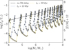 |
Fig. B.1. Impact of a coarse time sampling in determining the burstiness on the MZR for a system with Mdm = 3 × 10¹⁰ M⊙ at z = 6 evolved with our minimal physical model (cfr with Fig. 3). Different lines indicate different delay times for the SN feedback, as indicated in the legend. Squares (continuous lines) indicate a 2 Myr (0.2 Myr) time sampling. For visualization sake, the number of models is less than that present in Fig. 3. |
All Figures
|
Fig. 1. Mass-metallicity relation (MZR) at high redshift (z). We plot the gas metallicity (Zg) as a function of stellar mass (M⋆) for the SERRA simulated galaxies (Pallottini et al. 2022, z ≃ 7) and the JWST observations from CEERS Nakajima et al. (2023, z ≃ 4 − 10), JADES (Curti et al. 2024, z ≃ 3 − 6 and 6–10), and UNCOVER (Chemerynska et al. 2024b, z ≃ 6 − 8). To guide the eye, the observational fits from Nakajima et al. (2023) and Curti et al. (2024) are also reported as lines with the same colors of corresponding data. As a reference, the log(Zg/Z⊙) = 0.37 log(M⋆/M⊙)−4.3 fit from FIRE-2 simulations (Marszewski et al. 2024, z = 5 − 12) is shown, along with their binned data and scatter at z = 8. The right axis reports the logarithmic oxygen abundance [O/H], assuming a solar composition (Asplund et al. 2009), i.e., 12 + [O/H]⊙ = 8.69. |
| In the text | |
|
Fig. 5. SFR (σSFR, upper panel) and gas metallicity (σZ, lower panel) rms variations as a function of stellar mass for the sets of models presented in Fig. 4 (see Eqs. (3) for the definitions). As a reference, we report the SERRA average σSFR (Pallottini & Ferrara 2023) and σZ (this work), the σSFR from Ciesla et al. (2024), Mason et al. (2023), Muñoz et al. (2023), Shen et al. (2023), and the σZ for FIRE-2 at z = 8.0 (Marszewski et al. 2024) and JWST data. Note that ⟨JWST⟩ is the rms of the observations after subtraction of the fit to the MZR in the different datasets in Nakajima et al. (2023) and Curti et al. (2024); the thickness of the shaded area encloses the minimum and maximum of the rms of the different datasets. |
| In the text | |
|
Fig. 2. Example of the impact of SFR burstiness on the evolution of a galaxy hosted in a Mdm = 3 × 10¹⁰ M⊙ DM halo at z = 6 using the minimal physical model described in Sect. 3.1 (see in particular Eqs. (1)). The time evolution of the DM (black), star (green), gas (brown), and metal (pink) mass (M) content is shown with solid (dashed) lines for a SN-delay time of td = 10 Myr (td = 0, i.e. no delay). The upper axis shows the redshift, z, corresponding to cosmic time, t. |
| In the text | |
|
Fig. 3. Example of the impact of SFR burstiness on the MZR for a system with Mdm = 3 × 10¹⁰ M⊙ at z = 6 evolved with our minimal physical model. Different lines indicate different delay times for the SN feedback, as is indicated in the legend. Note that the model results have been resampled in 0.2 Myr steps and we do not consider the evolutionary phases when the galaxies have a negligible amount of gas (Mg ≤ 10−3 Mdm), which allows us to have a well-defined Zg even in periods when no gas and metals are present in the galaxy (see Fig. 2). For the effect of a coarser time sampling, see Appendix B, in particular Fig. B.1. |
| In the text | |
|
Fig. 4. Predicted MZR relation for different sets of minimal models with 109 M⊙ ≤ Mdm ≤ 1013 M⊙ halos at z = 6. In the upper left panel, we report the “base models” with ϵSN and td = 20 Myr (see Sect. 3.2). In the upper right panel, we modify the base model by reducing the efficiency of the feedback (ϵSN = 1/4 in Eq. (2a)). In the lower left panel, we consider both weak feedback and a cosmic accretion that is modulated on a timescale of 100 Myr (A100 = 1/3 in Eq. (4)). In the lower left panel, we show the effect of turning off the SN-delay for the weak feedback models with modulated cosmic accretion. In each panel, pastel lines are the individual tracks sampled every 2 Myr; their median and 16 − 84% dispersion are plotted with dashed and solid violet lines, respectively; the dashed black line is the control case with no-SN-delay (td = 0) and no modulated accretion (A100 = 0). For each model, we report the value values of the SFR flickering (σSFR) and the MZR dispersion (σZ, see Fig. 5). As in Fig. 1, we show JWST data and fits (Nakajima et al. 2023; Curti et al. 2024; Chemerynska et al. 2024b). |
| In the text | |
|
Fig. 6. Deviation from the FMR for high-z galaxies. We adopt the |
| In the text | |
|
Fig. A.1. Difference in the evolution of a Mdm = 3 × 10¹⁰ M⊙ computed by prescribing the fiducial ( |
| In the text | |
|
Fig. B.1. Impact of a coarse time sampling in determining the burstiness on the MZR for a system with Mdm = 3 × 10¹⁰ M⊙ at z = 6 evolved with our minimal physical model (cfr with Fig. 3). Different lines indicate different delay times for the SN feedback, as indicated in the legend. Squares (continuous lines) indicate a 2 Myr (0.2 Myr) time sampling. For visualization sake, the number of models is less than that present in Fig. 3. |
| In the text | |
Current usage metrics show cumulative count of Article Views (full-text article views including HTML views, PDF and ePub downloads, according to the available data) and Abstracts Views on Vision4Press platform.
Data correspond to usage on the plateform after 2015. The current usage metrics is available 48-96 hours after online publication and is updated daily on week days.
Initial download of the metrics may take a while.