| Issue |
A&A
Volume 696, April 2025
|
|
|---|---|---|
| Article Number | A203 | |
| Number of page(s) | 12 | |
| Section | Cosmology (including clusters of galaxies) | |
| DOI | https://doi.org/10.1051/0004-6361/202553709 | |
| Published online | 18 April 2025 | |
Detection of magnetic fields in superclusters of galaxies
1
Dipartimento di Fisica e Astronomia, Università degli Studi di Bologna, Via P. Gobetti 93/2, 40129 Bologna, Italy
2
INAF – Istituto di Radioastronomia, Via P. Gobetti 101, 40129 Bologna, Italy
3
Department of Physics and Electronics, Rhodes University, PO Box 94 Makhanda 6140, South Africa
4
Departamento de Física de la Tierra y Astrofísica & IPARCOS-UCM, Universidad Complutense de Madrid, 28040 Madrid, Spain
5
South African Radio Astronomy Observatory (SARAO), Black River Park, 2 Fir Street, Observatory, Cape Town 7925, South Africa
⋆ Corresponding author: This email address is being protected from spambots. You need JavaScript enabled to view it.
Received:
9
January
2025
Accepted:
8
March
2025
Abstract
Context. The properties of magnetic fields in large-scale structure filaments, far beyond galaxy clusters, are still poorly known. Superclusters of galaxies are laboratories for investigating low-density environments, which are not easily identified given the low signals and large scales involved. The observed Faraday rotation measure (RM) of polarised sources along the line of sight of superclusters allows us to constrain the magnetic field properties in these extended environments.
Aims. The aim of this work is to constrain the magnetic field intensity in low-density environments within the extent of superclusters of galaxies using the Faraday RM of polarised background sources detected at different frequencies.
Methods. We selected three rich and nearby (z < 0.1) superclusters of galaxies for which polarisation observations were available at both 1.4 GHz and 144 MHz: Corona Borealis, Hercules, and Leo. We compiled a catalogue of 4497 polarised background sources that have RM values either from the literature or derived from unpublished observations at 144 MHz. For each supercluster we created a 3D density cube in order to associate a density estimate with each RM measurement. We computed the median absolute deviation (MAD) variance of the RM values grouped in three density bins that correspond to the supercluster outskirts (0.01 < ρ/ρc < 1), filaments (1 < ρ/ρc < 30), and nodes (30 < ρ/ρc < 1000) regimes to investigate how variations in the RM distribution are linked to the mean density crossed by the polarised emission.
Results. We find an excess ΔσMAD2RRM = 2.5 ± 0.5 rad2 m−4 between the lowest-density regions (outside supercluster boundaries) and the low-density region inside the supercluster. This excess is attributed to the intervening medium of the filaments in the supercluster. We modelled the variance of the RM distribution as being due to a single-scale, randomly oriented magnetic field distribution and therefore as being dependant upon the magnetic field intensity along the line of sight, the magnetic field reversal scale, and the line-of-sight path length. Our observations do not constrain the latter two parameters, but if we marginalise over their respective prior range, we constrain the magnetic field to B|| = 19+50-8 nG.
Conclusions. Our findings are consistent with several other works that studied filaments of the large-scale structure. The results suggest that the purely adiabatic compression of a primordial magnetic field, which would imply observed magnetic fields of the order of B|| ∼ 2 nG, is not the only mechanism playing a role in amplifying the primordial seeds in superclusters of galaxies.
Key words: magnetic fields / polarization / galaxies: clusters: general / galaxies: clusters: intracluster medium / large-scale structure of Universe
© The Authors 2025
 Open Access article, published by EDP Sciences, under the terms of the Creative Commons Attribution License (https://creativecommons.org/licenses/by/4.0), which permits unrestricted use, distribution, and reproduction in any medium, provided the original work is properly cited.
This article is published in open access under the Subscribe to Open model. This email address is being protected from spambots. You need JavaScript enabled to view it. to support open access publication.
1. Introduction
The matter distribution of the Universe on megaparsec scales is not uniform or random: it is distributed according to a pattern called the cosmic web (Bond et al. 1996). Galaxies and galaxy clusters are found at the high-density ‘nodes’ of the cosmic web (ne ≪ 10−3 cm−3) and are connected by lower-density environments such as filaments (ne ∼ 10−6 − 10−4 cm−3). Filaments are thought to be permeated by the warm-hot intergalactic medium (Gheller et al. 2015) and have temperatures of 105 − 107 K and magnetic fields. While the magnetic field properties of galaxies and galaxy clusters and groups are well studied (Laing et al. 2008; van Weeren et al. 2019), the magnetic fields in the unprocessed gas in filaments and voids far beyond galaxy clusters are still poorly known. In recent years, several studies attempted to constrain the strength of magnetic fields in filaments using different approaches. Optical-IR galaxy distribution and radio cross-correlation (Vernstrom et al. 2017; Brown et al. 2017) and image-stacking studies (Tanimura et al. 2020; Vernstrom et al. 2021) have found estimates and limits ranging from 30 and 60 nG. With LOw-Frequency ARray (LOFAR) High Band Antenna observations, the non-detection of diffuse emission in filaments between galaxy clusters were used to determine upper limits ranging from ≤0.2 μG (Locatelli et al. 2021) to ≤0.75 μG (Hoang et al. 2023). Direct detection of the non-thermal synchrotron and X-ray emission associated with filaments of the cosmic web is possible (Vazza et al. 2019); this was confirmed by the discovery of two radio bridges of diffuse synchrotron emission between clusters (Govoni et al. 2019; Botteon et al. 2020) that had an estimated magnetic field of ∼0.3 μG in the inter-cluster region (Pignataro et al. 2024). However, these detections represent a ‘short’ population of filaments (∼1 − 5 Mpc) with overdensity ρ/ρc ∼ 2001 (e.g. Wittor et al. 2019), compressed by the dynamical activity between two merging clusters. Meanwhile, fainter filaments (ρ/ρc ∼ 10) on scales of several tens of megaparsecs remain undetected.
An alternative approach to measuring magnetic fields is to use the Faraday rotation of linearly polarised sources along the line of sight of a magnetised plasma. The Faraday rotation measure (RM) quantifies the rotation of the linear polarisation vector as a function of wavelength and depends on the line-of-sight magnetic field strength, B||, permeating a medium of ionised gas with electron density ne along a path length L between the source at redshift z and the observer:
![Mathematical equation: $$ \begin{aligned} \mathrm{RM} = 0.812 \int \frac{n_{\rm e}\,B_{||}}{(1+z)^2}\,\mathrm{d}L \quad [\mathrm{rad/m}^{2}]. \end{aligned} $$](/articles/aa/full_html/2025/04/aa53709-25/aa53709-25-eq2.gif) (1)
(1)
Vernstrom et al. (2023) recently reported a high polarisation fraction for short-range filaments (< 10 Mpc) in between massive halos, which implies a significantly ordered magnetic field component in these environments, consistent with the detection of an RM signal from them. Carretti et al. (2025) estimated magnetic fields of 10 − 145 nG with extragalactic RMs at low frequencies and overdensity ρ/ρc ∼ 10. At higher frequencies, RM studies report limits between 40 nG (Vernstrom et al. 2019) for extragalactic magnetic fields and 0.3 μG in superclusters of galaxies (Xu et al. 2006; Sankhyayan & Dabhade 2024). All these estimates and studies are of key importance in understanding the magneto-genesis scenarios in our Universe (Durrer & Neronov 2013; Subramanian 2016) because the filament environments preserve the memory of the primordial conditions while still being more easily detectable than voids (Vazza et al. 2017; Mtchedlidze et al. 2022). The investigation of magnetic fields in low-density environments (i.e. ne ∼ 10−5 cm−3) can help us distinguish between two main models: primordial scenarios, where the seed is produced during the early phases of inflation or before recombination (Paoletti & Finelli 2019), and astrophysical scenarios, where the feedback from active galactic nuclei (AGNs) is responsible for the late magnetisation of the Universe (Bertone et al. 2006; Donnert et al. 2009). One way to identify the location of filaments is to search for superclusters of galaxies: they are nested within the cosmic web and create a coherent structure of galaxy clusters embedded in a network of filaments spanning up to hundreds of megaparsecs (Lietzen et al. 2016; Bagchi et al. 2017). The possibility of finding filamentary structure increases within superclusters (Tanaka et al. 2007) because they have higher mean densities.
There are several different ways to identify superclusters in the sky, which makes them particularly useful when researching the large-scale structure of filaments. One frequently used approach is to exploit the galaxy overdensity distribution to trace filamentary structures connecting clusters and groups. This is facilitated by the vast availability of sky surveys such as the Sloan Digital Sky Survey (SDSS; Almeida et al. 2023), the Two Micron All Sky Survey (2MASS; Skrutskie et al. 2006), the Two Degree Field Redshift Survey (2dFRS; Huchra et al. 2012), and the Center for Astrophysics galaxy redshift survey (CfA2; Huchra et al. 1999). Superclusters of galaxies are frequently identified using the friends-of-friends algorithm (e.g. Zeldovich et al. 1982; Einasto et al. 1984; Chow-Martínez et al. 2014; Bagchi et al. 2017; Sankhyayan & Dabhade 2024), which is used to find and group points (in this case, galaxies) with unknown distributions in a simulation. Other methods are also used, such as applying a threshold cut to the luminosity density field of the galaxy distribution (Einasto et al. 2007; Lietzen et al. 2016) or to the number density field constructed via Voronoi tessellation (Neyrinck 2008; Nadathur & Crittenden 2016). Santiago-Bautista et al. (2020) developed an identification method based on geometrical information of the galaxy distribution. This process of identification resulted in several different catalogues of known superclusters of galaxies that can be used in combination with Faraday RM catalogues of sources behind superclusters to probe the magnetic field of the plasma crossed by the polarised emission of the distant radio sources (Xu et al. 2006; Sankhyayan & Dabhade 2024).
In this work we constrain the magnetic field intensity in filaments by using RM measurements of sources behind galaxy clusters. In Sect. 2 we present the available RM grid data and the construction of the polarised source catalogue behind the lines of sight of the selected superclusters. In Sect. 3 we show how we constructed the supercluster density maps and how we combined RM values from different surveys. In Sects. 4 and 4.1 we present the results of the analysis of the trend of residual rotation measure (RRM) variance and the gas density, and discuss different scenarios to constrain the magnetic fields in low-density environments. Finally, in Sect. 5 we summarise our findings.
2. Observations and dataset
In this section we describe the different datasets that were used in this work.
2.1. Selection of superclusters of galaxies
This work is based on the selection of polarised sources for which we have an RM value, in the line of sight of superclusters of galaxies. We based this study on the LOFAR Two-Metre Sky Survey (LoTSS) RM grid (O’Sullivan et al. 2023), which is sensitive to small RMs. Therefore, we selected nearby (z ≤ 0.1) superclusters in the northern sky that are covered, at least partially, by LoTSS observations. We chose to analyse three rich superclusters: Corona Borealis, Leo, and Hercules. These three superclusters are part of the all-sky Main SuperCluster Catalogue (MSCC; Chow-Martínez et al. 2014), which is a catalogue of 601 superclusters created with the combination of a compilation of the rich Abell clusters (Andernach et al. 2005) and spectroscopic redshifts for galaxies in the SDSS-DR7 (Abazajian et al. 2009). With a tunable Friends-of-Friends algorithm, Chow-Martínez et al. (2014) are able to provide a full list of the cluster members with their redshift, coordinates and supercluster membership out to a redshift of z = 0.15. This catalogue was further expanded by the analysis of Santiago-Bautista et al. (2020), where they select 46 MSCC clusters to map the elongated structures of low relative density inside each supercluster and they employ optical galaxies with spectroscopic redshifts from the SDSS-DR13 (Albareti et al. 2017). The SDSS galaxies are selected inside a volume of a box with ‘walls’ set to a distance of 20  Mpc from the centre of the farthest clusters in each direction, for each supercluster (Santiago-Bautista et al. 2020). Therefore, with this catalogue we were able to map the galaxy density over the supercluster volume as well as recover the redshift, virial radius, and location of each supercluster member (clusters and groups of galaxies). The properties of the selected superclusters, as reported in Santiago-Bautista et al. (2020), are summarised in Table 1, and the nominal location of each supercluster member on the sky is shown in Fig. 1.
MSCC supercluster properties.
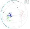 |
Fig. 1. Sky distribution of the members of each supercluster in the equatorial reference system. The location of the Galactic plane is shown in light blue. |
2.2. RM grids
Faraday RM grids are a valuable tool for studying the origin and evolution of cosmic magnetism, in particular by measuring the properties of extragalactic magnetic fields (Vernstrom et al. 2019; O’Sullivan et al. 2019). In this particular framework, we observe linearly polarised radio sources across a particular area of the sky, covered by the extension of a nearby supercluster, to investigate the Faraday rotation properties of the low-density, large-scale environments. To do this, we are mainly interested in the RM variance generated by the variations of the Faraday rotating medium along different lines of sight, due to either the intergalactic or local media. To isolate this component, it is necessary to remove the Galactic contribution from the Milky Way, and the errors introduced by the measurements. The RM variance has been investigated extensively with the 37543 RM values from the NRAO VLA Sky Survey (NVSS) data (Condon et al. 1998; Taylor et al. 2009) at 1.4 GHz, both to characterise the Milky Way properties (e.g. Purcell et al. 2015; Hutschenreuter & Enßlin 2020) and isolate the RM variance contribution local to the source itself (Rudnick & Blundell 2003; O’Sullivan et al. 2013; Anderson et al. 2018; Banfield et al. 2019; Knuettel et al. 2019).
RM studies at metre wavelengths offer a significant advantage over centimetre wavelength observations due to a better RM accuracy and sensitivity to low RM values. The accuracy of Faraday RMs is directly related to the wavelength-squared coverage, and thus RM studies at metre wavelengths provide substantially higher accuracy for individual RM measurements (Neld et al. 2018; O’Sullivan et al. 2018; Van Eck et al. 2018). Despite this, identifying linearly polarised sources at long wavelengths presents its own challenges; in particular, high angular resolution and high sensitivity are needed to counteract the significant effects of Faraday de-polarisation, which results in a smaller fraction of radio sources exhibiting detectable polarisation levels (e.g. Farnsworth et al. 2011; Bernardi et al. 2013; Lenc et al. 2017). LOFAR is addressing these challenges effectively with its capability to produce high-fidelity images at high angular resolution (Morabito et al. 2016; Jackson et al. 2016; Harris et al. 2019; Sweijen et al. 2022). Additionally, the LOFAR wide field of view and large instantaneous bandwidth facilitate the efficient surveying of large sky areas, aiding the detection of numerous linearly polarised sources and their RM values. The LoTSS-DR2 RM grid (O’Sullivan et al. 2013) has produced a catalogue of 2461 extragalactic high-precision RM values. The integration of RM grid catalogues from both metre and centimetre wavelengths is crucial for a more comprehensive understanding of the various contributors to Faraday rotation along the line of sight. We are interested in this combined approach, and we used both the NVSS and LoTSS RM grids to identify sources in the line of sight of our selected superclusters. The three superclusters have different extensions on the sky. We selected all sources inside a circle of radius 19° centred on each supercluster position. We checked for duplicates between NVSS and LoTSS RM sources and took the slight overlap between Corona Borealis and Hercules on the plane of the sky into account, which could introduce a number of additional duplicates. The duplicated RM were removed from the NVSS catalogue and kept in LoTSS catalogue, leaving us with 3679 RM values from the NVSS and 579 RM values from the LoTSS DR2 grid. For the 3679 NVSS RMs, we recomputed their overestimated  errors reported in Taylor et al. (2009), following the equation from Vernstrom et al. (2019):
 (2)
(2)
where P is the polarised intensity2 of the source and σP the associated error.
2.3. Source selection from non-DR2 fields
The selected superclusters are very extended across the sky, in particular Hercules (ID 474) and Leo (ID 278) can reach a declination as low as +3° (see Fig. 1). The LoTSS-DR2 sky area imaged in polarisation covers 5720 deg2 and it is split between two fields centred at 0h and 13h, respectively, down to a declination of approximately +15° (Shimwell et al. 2019; O’Sullivan et al. 2023). Therefore, part of these superclusters are not covered by the DR2. To improve the statistics and to find additional linearly polarised sources to probe the supercluster environments, we analysed an additional 177 LoTSS pointings not included the publicly available DR2 sky area. These RMs will form part of the LoTSS DR3 RM grid data release. The analysis of the additional pointings follow the same procedure used to create the LoTSS-DR2 RM grid, as reported in O’Sullivan et al. (2023). Here, we report the main steps:
-
We used Stokes Q and U image cubes at 20″ resolution and the Stokes I 20″ resolution images and source catalogues (Williams et al. 2019; Shimwell et al. 2022) from the LoTSS initial data products (Shimwell et al. 2019; Tasse et al. 2021);
-
The RM synthesis technique (Burn 1966; Brentjens & de Bruyn 2005) was applied on the Q and U images using RMsynt1D from RM-Tools3 (Purcell et al. 2020) with uniform weighting, for pixels in the Stokes I 20″ image where the total intensity was greater than 1 mJy beam−1. Initially, it is necessary to define a ‘leakage’ exclusion range between ±3 rad m−2 to remove the contamination of the instrumental polarisation in the Faraday depth spectrum or Faraday dispersion function (FDF). The leakage peak occurs intrinsically at 0 rad m−2 with a degree of polarisation of ≲1% of the Stokes I intensity (Shimwell et al. 2022), but it is shifted by the typical LOFAR ionospheric RM correction up to 3 rad m−2 (Sotomayor-Beltran et al. 2013; Šnidarić et al. 2023). To help reduce the effect of sidelobe structure, we ran the code RMclean1D (Purcell et al. 2020), which performs deconvolution of the FDF. With a variation of the Högbom CLEAN (Högbom 1974) algorithm, the RM-clean iteratively subtracts scaled versions of the RM spread function from the FDF until a noise threshold is reached (Heald et al. 2009, for a full description). We used a threshold of four times the noise in the FDF during the RM-clean process. From the clean spectrum and outside the leakage range, we identified the peak polarised intensity for each pixel in the output cube of the FDF.
-
We estimated the noise σQU and initially consider the Faraday depth (i.e. the RM) value corresponding the polarised intensity peaks in the FDF larger than 5.5σQU from the rms of the wings of the real and imaginary parts of the FDF (ϕ < −100 rad m−2 and ϕ > 100 rad m−2). Finally, an RM image, a polarised intensity image and a degree of polarisation map were created. From the polarised intensity image, all pixels within a box of 20 × 20 pixels and above the selected noise threshold, were grouped together. The highest signal to noise pixel in this group is the catalogued RM value and sky position of this source component.
An initial review of the catalogued sources revealed that many bright sources detected at small Faraday depths with very low degree of polarisation were likely instrumental peaks extending beyond the previously excluded leakage range. Consequently, to eliminate many of these sources we extended the leakage range to −5 rad m−2 < ϕ < +5 rad m−2 and excluded those sources with fractional polarisation smaller p < 2%, or very high values p > 30%. To be conservative, an 8σQU threshold was then applied following what is expected from false detection rates, which is as low as 10−4 at 8σQU, against a possible 4% at 5σQU (George et al. 2012). After these additional cuts, we inspected the Faraday spectra of the remaining sources. From the visual inspection of the FDF and the signal-to-noise ratio (S/N) it is possible to find some unreliable RM values that fell out the cuts. In particular, we inspected the FDF of sources very close to the acceptance threshold of 8σQU and checked the degree of polarisation. An example of accepted and rejected source after the visual inspection of the Faraday spectrum is shown in Fig. A.1. In this case, the rejected source satisfies the 8σQU criterium but the FDF shows the presence of several other peaks at a similar S/N level, making the detection unreliable.
The preliminary catalogue was then revised, and we noticed that some fields contained a high number of sources with very similar RM values and low polarisation fraction. This is likely attributable to a ‘transfer’ of polarised flux from a bright (> 10 mJy beam−1) polarised source in the field, as it was noticed in the original compilation of the LoTSS-DR2 RM grid (O’Sullivan et al. 2023). We therefore checked each field for this effect, and removed a total of 876 unreliable candidates from all fields.
After this step, we inspected also the maps produced after running the RM synthesis, and for each source we produced cutouts to compare the RM map, the polarised intensity image, the degree of polarisation map together with the Faraday spectrum and the NVSS 45″-resolution Stokes I and polarised intensity contours (see Fig. A.2). In this last step of inspection, we excluded sources with very complex Faraday spectrum where the peak is not clearly identified and/or is located at a pixel clearly outside the source, as well as sources with highly inconsistent LoTSS-NVSS degree of polarisation. This procedure excluded a few more sources. Finally, we removed duplicate sources from the NVSS, as done for the LoTSS-DR2 fields, keeping the RM value with higher S/N for LoTSS-LoTSS duplicates and LoTSS RM value for LoTSS-NVSS duplicates. The final non-DR2 catalogue contains 239 polarised source components, which we included in the analysis. Averaging together the three superclusters fields, we have a final catalogue4 with 3679 RM values from NVSS and 818 from LoTSS, for a total of 4497 polarised background sources.
3. Methods
3.1. Density maps
We used the final catalogue of polarised sources to study the supercluster medium by measuring the RM variance.
The RM variance is dependent on the free electron density, the line-of-sight magnetic field strength, and the magnetic field reversals that happen along the length of the path crossed by the radiation. Therefore, it is useful to relate the measured RM values to the density of the medium in the supercluster, and investigate which combinations of parameters will yield the observed variance. To limit the supercluster extent and estimate the density in each region, we used the gas density profile of each supercluster member. For this work, we chose to use the Universal gas density profile for galaxy clusters presented in Pratt et al. (2022). Using XMM-Newton observations, they derive an average intracluster medium density profile for a sample of 93 Sunyaev-Zeldovich effect -selected systems and determine its scaling with mass and redshift. The median radial profile is a function of a scaled radius x = R/R500, and is expressed as the product between a normalisation that can vary with the redshift z and the mass M500 (i.e. the total mass within the radius R500, i.e. when the mean matter density is 500 times the critical density of the Universe):
 (3)
(3)
where f(x) has the shape of a generalised Navarro-Frenk-White model (Nagai et al. 2007):
![Mathematical equation: $$ \begin{aligned} f(x) = \frac{f_0}{\left(\frac{x}{x_s}\right)^{\alpha } \left[1 + \left(\frac{x}{x_s}\right)^{\gamma }\right]^{\frac{3\beta - \alpha }{\gamma }}}\cdot \end{aligned} $$](/articles/aa/full_html/2025/04/aa53709-25/aa53709-25-eq8.gif) (4)
(4)
Here xs is the scaling radius, and the parameters α, β, and γ are the slopes at x ≪ xs, at x ≫ xs, and at x ∼ xs, respectively. The normalisation is given by the product of f0 and
![Mathematical equation: $$ \begin{aligned} N(z,M_{500})= E(z)^{\alpha _z}\left[\frac{M_{500}}{5\times 10^{14}\,M_{\odot }}\right]^{\alpha _M}, \end{aligned} $$](/articles/aa/full_html/2025/04/aa53709-25/aa53709-25-eq9.gif) (5)
(5)
where E(z) is the evolution of the Hubble parameter with redshift in a flat cosmology. A complete description of the fitting procedure to the 93 Sunyaev–Zeldovich-selected system can be found in Pratt et al. (2022), while here we only report the best-fit model parameters:
 (6)
(6)
The deprojected density profile with the best-fit parameters is applied to each supercluster member and computed radially for each element in a 3D cube of axis (RA, Dec and z). We zero-padded the density profile at distances ≥10 R500 from each cluster centre. With this approximation, we are treating all members as galaxy clusters, including small groups of galaxies down to five members; in this way, while the contribution of the smallest systems will have a low impact on the density at large distances from their centres, it helps trace the large-scale structure of the supercluster. We did not implement an additional density component for the filaments between clusters (see Sect. 4).
The construction of the density cubes for each supercluster allows us to describe the boundaries of the supercluster and investigate whether the radiation from the selected polarised background sources is crossing regions of high or low mean density, inside or outside the supercluster. Therefore, we computed a mean density ( ) along the direction of each radio source, averaged over the redshift interval of each cube, which allowed us to bin the sources in different density regimes. A 2D representation of the density maps for each supercluster is shown in Figs. 2, 3, and 4. It is noticeable how the sources found at 144 MHz have a smaller areal number density (0.43 deg−2; O’Sullivan et al. 2023) with respect to the ones found at 1.4 GHz (> 1 deg−2; Taylor et al. 2009). At both frequencies, sources are rarer in the highest-density regions, with ∼10% and ∼13% of the total number of sources found at mean densities ≳10−27.5 g cm−3, at 144 MHz and 1.4 GHz respectively (see Sect. 4.1). This is to be expected, due to the strong effect of Faraday depolarisation in galaxy clusters that is more important at lower frequencies (O’Sullivan et al. 2019; Carretti et al. 2022).
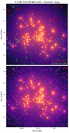 |
Fig. 2. 2D density map of the Corona Borealis supercluster, assuming that each member is on the same redshift plane. The location of the RM sources is shown in red for LoTSS-DR2, green for LoTSS non-DR2, and magenta for NVSS. |
With this selection, we are also probing the regions outside supercluster boundaries; the sources in the line of sight of very low-density environments serve as a control sample that allows us to quantify how the supercluster structure is contributing to the RM variance of the higher-density regions sources.
3.2. Statistics of the RM population
The accuracy with which we can isolate the effects of the supercluster structure on the RMs of the background sources depends on the size of our sample and the dispersion of the RM distribution. The measured RM is the combination of the Galactic RM (GRM) component, the extragalactic component (RMext), and a noise term. We are mainly interested in the extragalactic component, which can be attributed either to the local medium of the source (Laing et al. 2008) or to the foreground intergalactic medium. Therefore, we subtracted off the GRM component to be left with an RRM:
 (7)
(7)
where the GRM is estimated as the median of a disc of radius of 0.5° centred at the source position from the GRM map by Hutschenreuter et al. (2022) from several extragalactic source RM catalogues, including LoTSS and NVSS. Following Carretti et al. (2022), the choice of the radius is approximately the average spacing between sources in the catalogue suite used by Hutschenreuter et al. (2022). The median over a region can mitigate the possible effects of using sources that are part of the catalogue suite used to infer the GRM map, which results in the GRM at the exact source position being slightly biased towards the source RM (Carretti et al. 2022). While some residual contributions from GRM variations on smaller angular scales are possible, these are already mitigated by the large number of sources in our dataset, which cover different and extended regions of the sky, well away from the Galactic Plane (Fig. 1). Therefore, we are confident that by averaging over these sources, the potential scatter introduced by correlations does not necessarily introduce a systematic bias on the results.
We can estimate the RRM spread of the population, for example, with a median absolute deviation (MAD) statistic, which is less sensitive to outliers in a distribution. The MAD can be used analogously as the standard deviation (see e.g. Stuardi et al. 2021) to measure the dispersion of the distribution, by introducing a constant scale factor:
 (8)
(8)
where the value of k is taken assuming normally distributed data. Therefore, the intrinsic RRM MAD variance is obtained by subtracting the squared total noise term, consisting of the measurement term (σRM, err2) and the GRM error (σGRM, err2), from the observed RRM variance:
 (9)
(9)
As an indication, the typical measurement error for the RM in the selected LoTSS sources is ∼0.06 rad m−2, as opposed to ∼10 rad m−2 for the NVSS sources, while the average GRM error is ∼0.7 rad m−2. The combination of the LoTSS RM grid and NVSS RM catalogue can achieve a better sensitivity for the purpose of investigating the magnetic field strength and structure in superclusters. However, the different variances of the populations, for example, due to different survey sensitivities, frequency, foreground screens and background source properties must be properly weighted for them to be combined in the most effective manner (Rudnick 2019). In particular, we aim to give more weight to the sources that are better probes of the foreground medium in the supercluster, while minimising the local RM variations. One useful proxy of small RM scatter is the fractional polarisation of a radio source, which is dependent on both the intrinsic degree of order of the magnetic field and the Faraday depth structure across the emission region. Additionally, the presence of fluctuations on small scales can cause Faraday de-polarisation from the mixing of different polarisation vector orientations within the beam, which will reduce the fractional polarisation. The RM variance is directly linked to the Faraday de-polarisation, as expressed in Burn (1966) for an external screen:
 (10)
(10)
This will result in a correlation between fractional polarisation and de-polarisation (e.g. Stuardi et al. 2020). Higher fractional polarisation implies smaller RM variations due to the medium local to the source, and also smaller scatter in the RM distribution (Lamee et al. 2016). LoTSS detections are already preferentially selecting low de-polarisation sources with minimum Faraday complexity (O’Sullivan et al. 2023), which are excellent probes for our aim. However, the NVSS RM sources show more complexity and different polarisation structure due to the nature of the host galaxy (O’Sullivan et al. 2017). To reduce the effect of low fractional polarisation sources on the extragalactic RM variance, we can separate the NVSS sources into two populations, based on the median degree of polarisation of the sources in the NVSS RM catalogue (∼5%). Therefore, we weighed the three populations differently: LoTSS sources (population a), NVSS sources with high degree of polarisation (population b, p > 5%) and NVSS sources with low degree of polarisation (population c, p < 5%). Following Rudnick (2019), each population can be described with its own intrinsic RRM variance σi2 and a corresponding uncertainty, δi, calculated as
 (11)
(11)
where Ni is the number of sources of each population. We obtained the variance of the whole sample as the inverse-variance-weighted average of the variance of the three populations,
 (12)
(12)
and the total uncertainty,
 (13)
(13)
With this choice, the LoTSS sample will be weighted more than the NVSS sample.
4. Results and discussion
4.1. RRM variance versus density
We investigated the trend between the variations in the RRM distribution of the populations of sources through the line of sight of superclusters of galaxies and the density of the medium crossed by the polarised emission. As explained in Sects. 3.1 and 3.2, with the construction of the 3D density we are able to associate a mean value of density with each source in the field of the each supercluster, and we combined the different populations through a weighted average, where we specifically down-weighted the sources we expect to have a large RM variance in their local environments. As such, we can maximise the resulting accuracy of any possible RM signature from the superclusters by binning all the sources from the three superclusters in three main density regimes, thereby improving the MAD statistics.
The task of identifying and describing the cosmic web components has been undertaken through numerical simulations and observations with several different methods, both investigating the global pattern in a statistical way (see e.g. Peacock 1999; Hoyle et al. 2002; Colberg 2007) and segmenting the structure into its morphological components: voids, filaments, and clusters (e.g. Stoica et al. 2007, 2010; Genovese et al. 2010; González & Padilla 2010; Cautun et al. 2013). We can base our investigation of supercluster density regimes on the density distribution across cosmic environments presented in Cautun et al. (2014), where they show that various structures are characterised by different density values. The node regions, where clusters reside, typically have the highest densities (ρ/ρc ≥ 100) and filaments also represent over-dense regions spanning a wide range of density values (ρ/ρc ∼ 1 − 10), while voids are very under-dense (ρ/ρc ≤ 1/10). Although it is difficult to precisely define a density range to describe exactly the supercluster environments, we used these density regimes to define the bin ranges for our sources: specifically, the RRMs that have lines of sight inside the virial radii of the galaxy clusters (nodes) and those with lines of sight through the low-density gas inside the supercluster boundaries but outside the virial radii of clusters (filaments). We compared with the sources that fall outside the supercluster boundaries, assuming their RRMs can be attributed to typical extragalactic background. We used their RRMs to identify the contribution of the supercluster and investigate the magnetic fields in these regions.
We defined three starting bins based on the previous considerations: 10−31 < ρgas < 10−29 g cm−3 (0.01 < ρ/ρc < 1) for sources that can be considered outside supercluster boundaries, 10−29 < ρgas < 10−27.5 g cm−3 (1 < ρ/ρc < 30) for sources that are falling inside supercluster boundaries but outside galaxy clusters, and finally 10−27.5 < ρgas < 10−26 g cm−3 (30 < ρ/ρc < 1000) for sources that are inside galaxy clusters virial radii. For each bin, we computed the weighted MAD variance of RRMs from LoTSS, NVSS high-degree of polarisation, and NVSS low-degree of polarisation source populations (see Sect. 3.2). We show the resulting total weighted MAD variance (σMAD2RRM) as a function of the gas density in Fig. 5 (top panel). If we consider the RRMs variations of sources falling outside supercluster boundaries (first bin) to be mostly caused by the medium local to the source, then we can subtract the local contribution to the variance in the second bin to isolate the effect of the supercluster low-density regions. Between the first and second bin, we measure an excess RRM variance of ΔσMAD2RRM = 2.5 ± 0.5 rad2 m−4.
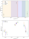 |
Fig. 5. Total weighted RRM MAD variance (σMAD2RRM) trend with gas density in superclusters of galaxies. The plot shows the resulting variance from binning the sources in different gas density regimes. The background is divided into the ranges of densities that are typically related to voids (yellow), filaments (blue), and nodes (green; Cautun et al. 2014). The dashed red line represents where the gas ρ200 limit would approximately be, to highlight the density trend outside galaxy clusters. We measure an excess in the RRM variance between the first and second density bins, which can be attributed to the contribution of the low-density magnetised gas in the supercluster structure. Bottom panel: Same as the top panel, but varying the bins edges with steps of 0.03 (−0.03) with respect the original chosen value. The different resulting MAD variances and their uncertainties are show in different colours. The weighted average of these results in each bin is shown in blue and is consistent with the original value, shown in black. |
To investigate the effect of the choice of bin boundaries in this detection, we varied the bin edges to shift the boundaries of different quantities and see the effect on the resulting variance. We chose to introduce a shift between 0.0 and 0.3 (−0.3) in ten equal logarithmic step. The results of this test are shown in Fig. 5 (bottom panel), where the results of each shift are marked in a different colour. The bin that is most affected by the choice of bin edges is the highest-density one, which exhibit very different results. It can be noted that moving the bin edge towards higher density values (i.e. towards galaxy cluster centres), the variance gets lower. This is consistent with the presence of only a few sources near cluster centres with low variance that survive de-polarisation effects. In general, this bin shows higher uncertainty due to the smaller number of sources (only 564 RMs, while 1195 and 2738 RMs in the first two bins) found at higher densities for de-polarisation effects (see e.g. Bonafede et al. 2011; Böhringer et al. 2016; Osinga et al. 2022), and therefore we did not include these regions in our analysis. If we compute the weighted average of the resulting σMAD and their uncertainties, we find that the first two bin results are in agreement with the starting value.
4.2. Constraints on supercluster magnetic fields
With the detection of an excess in RRM variance that can be attributed to the supercluster structure, we attempted to estimate the required field strength permeating the low-density environments crossed by the polarised emission. The variance of the RRM distribution (σth2) for a single-scale model of a randomly oriented field structure can be described by a simple model (Murgia et al. 2004):
 (14)
(14)
where Λc is the magnetic field reversal scale, ne is the gas electron number density, and B|| is the magnetic field over any line of sight through the supercluster over a path length L. The model σth2RRM can be computed as Eq. (14) for different values of the parameters (Λc, B||, L) and compared with the measured  (RRM) at the densities in the first two bins as derived in Sect. 4.1.
We adopted a Bayesian Monte Carlo sampling (e.g. Monte Carlo Markov chain) approach to explore the likelihood surface and reconstruct the posterior distribution of the free parameters (Λc, B||, and L). In the modelling framework, we call the data d and the model parameters m and write the Bayes theorem (up to a constant) as
 (15)
(15)
This relates the posterior probability function of the parameters P(m ∣ d) to the likelihood function ℒ(d ∣ m), which we would like to maximise, and the prior Π, which encodes existing knowledge of parameter values. In our case, we can write the likelihood function of detecting the observed σMAD2RRM(ne) for a medium of density ne as
![Mathematical equation: $$ \begin{aligned} \mathcal{L} \left(\sigma _{\rm MAD}^{2_{\rm RRM}} \mid \boldsymbol{m}\right) \propto \exp \left[-\frac{1}{2}\sum _i\left(\frac{\sigma ^{2_{\rm RRM}}_{\rm MAD}(n_{\mathrm{e},i}) - \sigma _{\rm th}^{2_{\rm RRM}}(n_{\mathrm{e},i}, \boldsymbol{m})}{\delta (n_{\mathrm{e},i})}\right)^2\right], \end{aligned} $$](/articles/aa/full_html/2025/04/aa53709-25/aa53709-25-eq22.gif) (16)
(16)
where δ is the uncertainty on the i-th measured values of  and m = (Λc, B||, L). For the parameters, we assumed flat priors in ranges 0 ≤ B|| ≤ 2 μG, 5 ≤ Λc ≤ 500 kpc, and 5 ≤ L ≤ 70 Mpc. While the choice of the parameters ranges is arbitrary given the limited information on supercluster environments, it is dictated by some reasonable considerations: the magnetic field strength is investigated up to values found in galaxy clusters (a few microgauss; e.g. Bonafede et al. 2010; Govoni et al. 2017); the magnetic field will fluctuate on a range of scales, and therefore we investigated out to a large outer scale of Λc = 500 kpc (Enßlin & Vogt 2003; Murgia et al. 2004; Vacca et al. 2010); finally, the maximum path length through the supercluster is computed following as the average of the three superclusters box size (∼70 Mpc) defined in Santiago-Bautista et al. (2020) that enclose each supercluster structure (see Table 1).
The distribution is then sampled with Monte Carlo Markov chains using emcee (Foreman-Mackey et al. 2013). Figure 6 shows the posterior probability distributions, marginalised into one and two dimensions, for the model parameters. The distributions for each parameter are plotted along the diagonal and covariances between them under the diagonal. The shape of the covariance indicate the correlation between the parameters, namely a circular or diffuse covariance means no correlation, while elongated shapes can show correlation. As expected from Eq. (14), the path length L and the reversal scale Λc are essentially unconstrained within the prior range. The posterior distribution of the magnetic field shows correlation with the two other parameters but, once marginalised over them, shows a Gaussian-like behaviour, though skewed towards high values. As shown in Fig. 7, we can constrain  nG, different from zero with a confidence level larger than 95%.
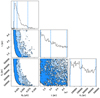 |
Fig. 6. Posterior probability distribution, marginalised into one and two dimensions, for the parameters B||, L, and Λc. Dark and light blue shaded areas indicate the 68 and 95% confidence regions. The 1D projection for each parameters is shown at the top. The dashed blue lines represent (from left to right) the 2.5th, 50th, and 97.5th percentiles. |
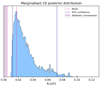 |
Fig. 7. Magnetic field marginalised posterior distribution, zoomed-in from Fig. 6. The distribution is skewed towards small values. The 95% confidence levels of the distribution are shown in dashed blue. The most likely value is shown in dashed red. The resulting adiabatic compression level is shown in purple. |
This result for the magnetic field in low-density regions of superclusters is in agreement with what is found with different methods investigating the filaments of the cosmic web (Carretti et al. 2022, 2023; Vernstrom et al. 2023) and preliminary studies on superclusters with Faraday RMs (Xu et al. 2006; Sankhyayan & Dabhade 2024). Moreover, some early works on simulations have investigated the contribution of large-scale structure filaments to the RM of background sources. These simulations suggest that the magnetic field intensity in filaments could range from 10 nG to 100 nG (Ryu et al. 2008; Cho & Ryu 2009; Akahori & Ryu 2010; Vazza et al. 2015), which still is in agreement with our findings.
In our analysis we considered the density contribution from supercluster members only and, therefore, neglected the possible filament contribution and, in turn, overestimated the magnetic field intensity. While a better approach may be to compare directly with simulations of the RM variations from supercluster structures, we can estimate the effect of including an additional density component by increasing the density of the second bin (see Fig. 5) with a 20% excess from filaments, as recently measured with profiles of the Sunyaev–Zeldovich signal from stacked galaxy pairs (de Graaff et al. 2019). The resulting magnetic field is consistent with the initial finding, and therefore still comparable with works of large-scale structure filaments.
Constraints on the magnetic field strength in cosmic structures are of key importance to investigate magneto-genesis scenarios. For this purpose, ad hoc cosmological simulation of superclusters are needed but not available yet. However, we can compute a preliminary estimate of the predicted adiabatic compression-only effect on a primordial seed and compare with our results. For adiabatic compression, the magnetic field strength scales with density as B = B0(n/n0)2/3. With an initial seed of cosmological origin, as derived from the analysis of cosmic microwave background anisotropies (i.e. B0 ∼ 2 nG; Planck Collaboration XIII 2016) compression seems enough to explain the magnetic field strength derived in this analysis. However, recent LOFAR RRM measurements in intergalactic medium filaments suggest magnetic field seeds more than an order of magnitude below the limit derived with cosmic microwave background (Neronov et al. 2024). Assuming an initial seed of B0 ∼ 0.11 nG (Carretti et al. 2023) at mean critical baryonic density of n0 ∼ 4 × 10⁻³¹ g cm−3, the adiabatic compression to the density n ∼ 5 × 10⁻²⁹ g cm−3 as in our case, would yield B ∼ 3.5 nG, and  nG. Comparing the adiabatic compression effect to the resulting B|| from our analysis (see Fig. 7), it suggests that in superclusters of galaxies may be at play different mechanism such as dynamo amplification or AGN feedback, to further amplify the magnetic fields from ∼2 nG to the measured ∼20 nG. Another possible amplification mechanism is the presence of accretion strong shocks surrounding the filaments of the cosmic web, as observed in Vernstrom et al. (2023).
Since our result is dependent on the chosen Λc parameter range, we can try to set an additional constrain on the reversal scale length by fixing the path length to L = 70, the largest value considered for the parameter range. In this way, to reproduce the same RRM variance, we would minimise the magnetic field. The contour plot in Fig. 8 shows the 2D posterior distribution between B|| and Λc once L is fixed to 70 Mpc. In the case of the maximum path length through the superclusters, the magnetic field is still larger than what is predicted by adiabatic-compression only for all values of Λc. A strong constrain on Λc would result in the minimum line-of-sight magnetic field component in the supercluster environment.
 |
Fig. 8. Covariance between the magnetic field strength (B||) and reversal scale (Λc), with the path length fixed to L = 70 Mpc. The distribution 1 and 2σ contour levels are shown in black. The dashed red line represent the magnetic field resulting from adiabatic compression only. |
5. Conclusions
The Faraday RM signal from distant polarised sources is a sensitive probe of the foreground, extragalactic low-density gas that permeates the large-scale structure, which is difficult to detect otherwise. In this work, we made use of the NVSS and LoTSS RM catalogues, combining the large number of sources found at centimetre wavelengths with the highest precision of the sources detected at metre wavelengths to investigate the rarefied environments of three major superclusters of galaxies in the northern sky: Corona Borealis, Hercules, and Leo. Our findings can be summarised as follows:
-
For each supercluster we built a density 3D map (RA, Dec, z), computing the universal gas density profile (Pratt et al. 2022) for each member.
-
We created a catalogue of the 4497 polarised sources found in the background of the three superclusters. Among these, 3697 RM values are from the NVSS (Taylor et al. 2009) and 818 are from LoTSS (O’Sullivan et al. 2023). At the location of each source, we computed the mean gas density crossed by the polarised emission passing through the supercluster. We subtracted the Galactic contribution to investigate the extragalactic component. We then had for each source a pair of RRM and associated density values.
-
We computed the MAD variance of the RRM distribution in three different density regimes: voids, filaments, and nodes. While the highest-density bin (inside the galaxy cluster virial radii) is difficult to interpret due to several de-polarisation effects at play and low-number statistics, we detect an excess RRM variance of ΔσMAD2RRM = 2.5 ± 0.5 rad2 m−4 between the lowest-density region (outside the supercluster boundaries) and the low-density region inside the supercluster. We attribute this excess to the intervening medium of the filaments in the supercluster.
-
We estimated the required magnetic field strength permeating the low-density environments crossed by the polarised emission through a Bayesian approach. We infer a line-of-sight magnetic field strength of
 nG, while other quantities such as the path length and the magnetic field reversal scale remain unconstrained. Our result is in line with other work conducted on the filaments of the large-scale structure (e.g. Vernstrom et al. 2021; Carretti et al. 2022, 2023). Assuming only the effect of adiabatic compression from a primordial seed field consistent with current upper limits from LOFAR RRM measurements in intergalactic medium filaments (Neronov et al. 2024) would give B|| ∼ 2 nG. Our result suggests that in superclusters of galaxies, different mechanisms of magnetic field amplification may be at play, such as dynamo amplification or AGN or galaxy feedback, or that an additional primordial seed should be considered.
ρc = 3H02/8πG is the mean critical density of the Universe.
The polarised intensity is defined as  , where Q and U are the Stokes parameters.
The catalogue will be made available through Vizier.
Acknowledgments
SPO acknowledges support from the Comunidad de Madrid Atracción de Talento program via grant 2022-T1/TIC-23797, and grant PID2023-146372OB-I00 funded by MICIU/AEI/10.13039/501100011033 and by ERDF, EU. AB acknowledges financial support from the ERC Starting Grant ‘DRANOEL’, number 714245. FV acknowledges the support by Fondazione Cariplo and Fondazione CDP, through grant n° Rif: 2022-2088 CUP J33C22004310003 for “BREAKTHRU” project.
References
- Abazajian, K. N., Adelman-McCarthy, J. K., Agüeros, M. A., et al. 2009, ApJS, 182, 543 [Google Scholar]
- Akahori, T., & Ryu, D. 2010, ApJ, 723, 476 [NASA ADS] [CrossRef] [Google Scholar]
- Albareti, F. D., Allende Prieto, C., Almeida, A., et al. 2017, ApJS, 233, 25 [Google Scholar]
- Almeida, A., Anderson, S. F., Argudo-Fernández, M., et al. 2023, ApJS, 267, 44 [NASA ADS] [CrossRef] [Google Scholar]
- Andernach, H., Tago, E., Einasto, M., Einasto, J., & Jaaniste, J. 2005, ASP Conf. Ser., 329, 283 [NASA ADS] [Google Scholar]
- Anderson, C. S., Gaensler, B. M., Heald, G. H., et al. 2018, ApJ, 855, 41 [NASA ADS] [CrossRef] [Google Scholar]
- Bagchi, J., Sankhyayan, S., Sarkar, P., et al. 2017, ApJ, 844, 25 [NASA ADS] [CrossRef] [Google Scholar]
- Banfield, J. K., O’Sullivan, S. P., Wieringa, M. H., & Emonts, B. H. C. 2019, MNRAS, 482, 5250 [NASA ADS] [CrossRef] [Google Scholar]
- Bernardi, G., Greenhill, L. J., Mitchell, D. A., et al. 2013, ApJ, 771, 105 [Google Scholar]
- Bertone, S., Vogt, C., & Enßlin, T. 2006, MNRAS, 370, 319 [NASA ADS] [Google Scholar]
- Böhringer, H., Chon, G., & Kronberg, P. P. 2016, A&A, 596, A22 [NASA ADS] [CrossRef] [EDP Sciences] [Google Scholar]
- Bonafede, A., Feretti, L., Murgia, M., et al. 2010, A&A, 513, A30 [NASA ADS] [CrossRef] [EDP Sciences] [Google Scholar]
- Bonafede, A., Govoni, F., Feretti, L., et al. 2011, A&A, 530, A24 [CrossRef] [EDP Sciences] [Google Scholar]
- Bond, J. R., Kofman, L., & Pogosyan, D. 1996, Nature, 380, 603 [NASA ADS] [CrossRef] [Google Scholar]
- Botteon, A., van Weeren, R. J., Brunetti, G., et al. 2020, MNRAS, 499, L11 [Google Scholar]
- Brentjens, M. A., & de Bruyn, A. G. 2005, A&A, 441, 1217 [NASA ADS] [CrossRef] [EDP Sciences] [Google Scholar]
- Brown, S., Kaaret, P., & Zajczyk, A. 2017, Res. Notes Am. Astron. Soc., 1, 17 [Google Scholar]
- Burn, B. J. 1966, MNRAS, 133, 67 [Google Scholar]
- Carretti, E., Vacca, V., O’Sullivan, S. P., et al. 2022, MNRAS, 512, 945 [NASA ADS] [CrossRef] [Google Scholar]
- Carretti, E., O’Sullivan, S. P., Vacca, V., et al. 2023, MNRAS, 518, 2273 [Google Scholar]
- Carretti, E., Vazza, F., O’Sullivan, S. P., et al. 2025, A&A, 693, A208 [NASA ADS] [CrossRef] [EDP Sciences] [Google Scholar]
- Cautun, M., van de Weygaert, R., & Jones, B. J. T. 2013, MNRAS, 429, 1286 [NASA ADS] [CrossRef] [Google Scholar]
- Cautun, M., van de Weygaert, R., Jones, B. J. T., & Frenk, C. S. 2014, MNRAS, 441, 2923 [Google Scholar]
- Cho, J., & Ryu, D. 2009, ApJ, 705, L90 [Google Scholar]
- Chow-Martínez, M., Andernach, H., Caretta, C. A., & Trejo-Alonso, J. J. 2014, MNRAS, 445, 4073 [Google Scholar]
- Colberg, J. M. 2007, MNRAS, 375, 337 [NASA ADS] [CrossRef] [Google Scholar]
- Condon, J. J., Cotton, W. D., Greisen, E. W., et al. 1998, AJ, 115, 1693 [Google Scholar]
- de Graaff, A., Cai, Y.-C., Heymans, C., & Peacock, J. A. 2019, A&A, 624, A48 [NASA ADS] [CrossRef] [EDP Sciences] [Google Scholar]
- Donnert, J., Dolag, K., Lesch, H., & Müller, E. 2009, MNRAS, 392, 1008 [NASA ADS] [CrossRef] [Google Scholar]
- Durrer, R., & Neronov, A. 2013, A&ARv, 21, 62 [NASA ADS] [CrossRef] [Google Scholar]
- Einasto, J., Klypin, A. A., Saar, E., & Shandarin, S. F. 1984, MNRAS, 206, 529 [Google Scholar]
- Einasto, J., Einasto, M., Saar, E., et al. 2007, A&A, 462, 397 [NASA ADS] [CrossRef] [EDP Sciences] [Google Scholar]
- Enßlin, T. A., & Vogt, C. 2003, A&A, 401, 835 [NASA ADS] [CrossRef] [EDP Sciences] [Google Scholar]
- Farnsworth, D., Rudnick, L., & Brown, S. 2011, AJ, 141, 191 [NASA ADS] [CrossRef] [Google Scholar]
- Foreman-Mackey, D., Hogg, D. W., Lang, D., & Goodman, J. 2013, PASP, 125, 306 [Google Scholar]
- Genovese, C. R., Perone-Pacifico, M., Verdinelli, I., & Wasserman, L. 2010, ArXiv e-prints [arXiv:1003.5536] [Google Scholar]
- George, S. J., Stil, J. M., & Keller, B. W. 2012, PASA, 29, 214 [Google Scholar]
- Gheller, C., Vazza, F., Favre, J., & Brüggen, M. 2015, MNRAS, 453, 1164 [Google Scholar]
- González, R. E., & Padilla, N. D. 2010, MNRAS, 407, 1449 [CrossRef] [Google Scholar]
- Govoni, F., Murgia, M., Vacca, V., et al. 2017, A&A, 603, A122 [NASA ADS] [CrossRef] [EDP Sciences] [Google Scholar]
- Govoni, F., Orrù, E., Bonafede, A., et al. 2019, Science, 364, 981 [Google Scholar]
- Harris, D. E., Moldón, J., Oonk, J. R. R., et al. 2019, ApJ, 873, 21 [Google Scholar]
- Heald, G., Braun, R., & Edmonds, R. 2009, A&A, 503, 409 [NASA ADS] [CrossRef] [EDP Sciences] [Google Scholar]
- Hoang, D. N., Brüggen, M., Zhang, X., et al. 2023, MNRAS, 523, 6320 [CrossRef] [Google Scholar]
- Högbom, J. A. 1974, A&AS, 15, 417 [Google Scholar]
- Hoyle, F., Vogeley, M. S., Gott, J. R., et al. 2002, ApJ, 580, 663 [Google Scholar]
- Huchra, J. P., Vogeley, M. S., & Geller, M. J. 1999, ApJS, 121, 287 [Google Scholar]
- Huchra, J. P., Macri, L. M., Masters, K. L., et al. 2012, ApJS, 199, 26 [Google Scholar]
- Hutschenreuter, S., & Enßlin, T. A. 2020, A&A, 633, A150 [EDP Sciences] [Google Scholar]
- Hutschenreuter, S., Anderson, C. S., Betti, S., et al. 2022, A&A, 657, A43 [NASA ADS] [CrossRef] [EDP Sciences] [Google Scholar]
- Jackson, N., Tagore, A., Deller, A., et al. 2016, A&A, 595, A86 [NASA ADS] [CrossRef] [EDP Sciences] [Google Scholar]
- Knuettel, S., O’Sullivan, S. P., Curiel, S., & Emonts, B. H. C. 2019, MNRAS, 482, 4606 [NASA ADS] [CrossRef] [Google Scholar]
- Laing, R. A., Bridle, A. H., Parma, P., & Murgia, M. 2008, MNRAS, 391, 521 [NASA ADS] [CrossRef] [Google Scholar]
- Lamee, M., Rudnick, L., Farnes, J. S., et al. 2016, ApJ, 829, 5 [NASA ADS] [CrossRef] [Google Scholar]
- Lenc, E., Anderson, C. S., Barry, N., et al. 2017, PASA, 34, e040 [Google Scholar]
- Lietzen, H., Tempel, E., Liivamägi, L. J., et al. 2016, A&A, 588, L4 [NASA ADS] [CrossRef] [EDP Sciences] [Google Scholar]
- Locatelli, N., Vazza, F., Bonafede, A., et al. 2021, A&A, 652, A80 [NASA ADS] [CrossRef] [EDP Sciences] [Google Scholar]
- Morabito, L. K., Deller, A. T., Röttgering, H., et al. 2016, MNRAS, 461, 2676 [Google Scholar]
- Mtchedlidze, S., Domínguez-Fernández, P., Du, X., et al. 2022, ApJ, 929, 127 [NASA ADS] [CrossRef] [Google Scholar]
- Murgia, M., Govoni, F., Feretti, L., et al. 2004, A&A, 424, 429 [NASA ADS] [CrossRef] [EDP Sciences] [Google Scholar]
- Nadathur, S., & Crittenden, R. 2016, ApJ, 830, L19 [CrossRef] [Google Scholar]
- Nagai, D., Kravtsov, A. V., & Vikhlinin, A. 2007, ApJ, 668, 1 [Google Scholar]
- Neld, A., Horellou, C., Mulcahy, D. D., et al. 2018, A&A, 617, A136 [NASA ADS] [CrossRef] [EDP Sciences] [Google Scholar]
- Neronov, A., Vazza, F., Mtchedlidze, S., & Carretti, E. 2024, ArXiv e-prints [arXiv:2412.14825] [Google Scholar]
- Neyrinck, M. C. 2008, MNRAS, 386, 2101 [CrossRef] [Google Scholar]
- Osinga, E., van Weeren, R. J., Andrade-Santos, F., et al. 2022, A&A, 665, A71 [NASA ADS] [CrossRef] [EDP Sciences] [Google Scholar]
- O’Sullivan, S. P., Feain, I. J., McClure-Griffiths, N. M., et al. 2013, ApJ, 764, 162 [CrossRef] [Google Scholar]
- O’Sullivan, S. P., Purcell, C. R., Anderson, C. S., et al. 2017, MNRAS, 469, 4034 [CrossRef] [Google Scholar]
- O’Sullivan, S. P., Brüggen, M., Van Eck, C. L., et al. 2018, Galaxies, 6, 126 [CrossRef] [Google Scholar]
- O’Sullivan, S. P., Machalski, J., Van Eck, C. L., et al. 2019, A&A, 622, A16 [NASA ADS] [CrossRef] [EDP Sciences] [Google Scholar]
- O’Sullivan, S. P., Shimwell, T. W., Hardcastle, M. J., et al. 2023, MNRAS, 519, 5723 [CrossRef] [Google Scholar]
- Paoletti, D., & Finelli, F. 2019, JCAP, 2019, 028 [CrossRef] [Google Scholar]
- Peacock, J. A. 1999, Cosmological Physics (Cambridge: Cambridge University Press) [Google Scholar]
- Pignataro, G. V., Bonafede, A., Bernardi, G., et al. 2024, A&A, 682, A105 [NASA ADS] [CrossRef] [EDP Sciences] [Google Scholar]
- Planck Collaboration XIII. 2016, A&A, 594, A13 [NASA ADS] [CrossRef] [EDP Sciences] [Google Scholar]
- Pratt, G. W., Arnaud, M., Maughan, B. J., & Melin, J. B. 2022, A&A, 665, A24 [NASA ADS] [CrossRef] [EDP Sciences] [Google Scholar]
- Purcell, C. R., Gaensler, B. M., Sun, X. H., et al. 2015, ApJ, 804, 22 [NASA ADS] [CrossRef] [Google Scholar]
- Purcell, C. R., Van Eck, C. L., West, J., Sun, X. H., & Gaensler, B. M. 2020, Astrophysics Source Code Library [record ascl:2005.003] [Google Scholar]
- Rudnick, L. 2019, ArXiv e-prints [arXiv:1901.09074] [Google Scholar]
- Rudnick, L., & Blundell, K. M. 2003, ApJ, 588, 143 [NASA ADS] [CrossRef] [Google Scholar]
- Ryu, D., Kang, H., Cho, J., & Das, S. 2008, Science, 320, 909 [NASA ADS] [CrossRef] [Google Scholar]
- Sankhyayan, S., & Dabhade, P. 2024, A&A, 687, L8 [NASA ADS] [CrossRef] [EDP Sciences] [Google Scholar]
- Santiago-Bautista, I., Caretta, C. A., Bravo-Alfaro, H., Pointecouteau, E., & Andernach, H. 2020, A&A, 637, A31 [NASA ADS] [CrossRef] [EDP Sciences] [Google Scholar]
- Shimwell, T. W., Tasse, C., Hardcastle, M. J., et al. 2019, A&A, 622, A1 [NASA ADS] [CrossRef] [EDP Sciences] [Google Scholar]
- Shimwell, T. W., Hardcastle, M. J., Tasse, C., et al. 2022, A&A, 659, A1 [NASA ADS] [CrossRef] [EDP Sciences] [Google Scholar]
- Skrutskie, M. F., Cutri, R. M., Stiening, R., et al. 2006, AJ, 131, 1163 [NASA ADS] [CrossRef] [Google Scholar]
- Šnidarić, I., Jelić, V., Mevius, M., et al. 2023, A&A, 674, A119 [NASA ADS] [CrossRef] [EDP Sciences] [Google Scholar]
- Sotomayor-Beltran, C., Sobey, C., Hessels, J. W. T., et al. 2013, A&A, 552, A58 [NASA ADS] [CrossRef] [EDP Sciences] [Google Scholar]
- Stoica, R. S., Martínez, V. J., & Saar, E. 2007, J. Roy. Stat. Soc.: Ser. C (Appl. Stat.), 56, 1 [Google Scholar]
- Stoica, R. S., Martínez, V. J., & Saar, E. 2010, A&A, 510, A38 [CrossRef] [EDP Sciences] [Google Scholar]
- Stuardi, C., O’Sullivan, S. P., Bonafede, A., et al. 2020, A&A, 638, A48 [EDP Sciences] [Google Scholar]
- Stuardi, C., Bonafede, A., Lovisari, L., et al. 2021, MNRAS, 502, 2518 [NASA ADS] [CrossRef] [Google Scholar]
- Subramanian, K. 2016, Rep. Progr. Phys., 79, 076901 [CrossRef] [Google Scholar]
- Sweijen, F., van Weeren, R. J., Röttgering, H. J. A., et al. 2022, Nat. Astron., 6, 350 [NASA ADS] [CrossRef] [Google Scholar]
- Tanaka, M., Hoshi, T., Kodama, T., & Kashikawa, N. 2007, MNRAS, 379, 1546 [NASA ADS] [CrossRef] [Google Scholar]
- Tanimura, H., Aghanim, N., Kolodzig, A., Douspis, M., & Malavasi, N. 2020, A&A, 643, L2 [EDP Sciences] [Google Scholar]
- Tasse, C., Shimwell, T., Hardcastle, M. J., et al. 2021, A&A, 648, A1 [EDP Sciences] [Google Scholar]
- Taylor, A. R., Stil, J. M., & Sunstrum, C. 2009, ApJ, 702, 1230 [Google Scholar]
- Vacca, V., Murgia, M., Govoni, F., et al. 2010, A&A, 514, A71 [CrossRef] [EDP Sciences] [Google Scholar]
- Van Eck, C. L., Haverkorn, M., Alves, M. I. R., et al. 2018, A&A, 613, A58 [NASA ADS] [CrossRef] [EDP Sciences] [Google Scholar]
- van Weeren, R. J., de Gasperin, F., Akamatsu, H., et al. 2019, Space Sci. Rev., 215, 16 [Google Scholar]
- Vazza, F., Ferrari, C., Brüggen, M., et al. 2015, A&A, 580, A119 [NASA ADS] [CrossRef] [EDP Sciences] [Google Scholar]
- Vazza, F., Brüggen, M., Gheller, C., et al. 2017, Class. Quant. Grav., 34, 234001 [Google Scholar]
- Vazza, F., Ettori, S., Roncarelli, M., et al. 2019, A&A, 627, A5 [NASA ADS] [CrossRef] [EDP Sciences] [Google Scholar]
- Vernstrom, T., Gaensler, B. M., Brown, S., Lenc, E., & Norris, R. P. 2017, MNRAS, 467, 4914 [NASA ADS] [CrossRef] [Google Scholar]
- Vernstrom, T., Gaensler, B. M., Rudnick, L., & Andernach, H. 2019, ApJ, 878, 92 [NASA ADS] [CrossRef] [Google Scholar]
- Vernstrom, T., Heald, G., Vazza, F., et al. 2021, MNRAS, 505, 4178 [NASA ADS] [CrossRef] [Google Scholar]
- Vernstrom, T., West, J., Vazza, F., et al. 2023, Sci. Adv., 9, eade7233 [NASA ADS] [CrossRef] [Google Scholar]
- Williams, W. L., Hardcastle, M. J., Best, P. N., et al. 2019, A&A, 622, A2 [NASA ADS] [CrossRef] [EDP Sciences] [Google Scholar]
- Wittor, D., Domínguez-Fernández, P., Vazza, F., & Brüggen, M. 2019, ArXiv e-prints [arXiv:1909.10792] [Google Scholar]
- Xu, Y., Kronberg, P. P., Habib, S., & Dufton, Q. W. 2006, ApJ, 637, 19 [NASA ADS] [CrossRef] [Google Scholar]
- Zeldovich, I. B., Einasto, J., & Shandarin, S. F. 1982, Nature, 300, 407 [Google Scholar]
Appendix A: Inspection of FDF for source selection
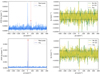 |
Fig. A.1. Absolute value of the Faraday spectrum (FDF; solid blue line) and the real (Q; solid green line) and imaginary (U; solid yellow line) components of the FDF, for two example polarised source components. The Q,U plots have a restricted range on the y-axis to better visualise the noise. The ‘real’ peak, i.e. the highest signal-to-noise polarised component outside the leakage range, is marked with a red cross. The leakage peak is noticeable in both cases at ϕ ∼ 0 rad m−2. The rms noise (σQU) level is shown as a dashed line. After inspection, the top source at S/N ∼ 8 is excluded, while the bottom source, at S/N ∼ 40 is accepted. |
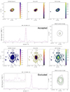 |
Fig. A.2. Inspection maps to evaluate the catalogued polarised source component. Top row: LoTSS 20″ resolution RM map, degree of polarisation map, and polarised intensity map for the catalogued source inside the Stokes I contours (black). Bottom row: FDF with the catalogued RM value and S/N for the peak, and the NVSS 45″ resolution Stokes I (black) and polarised intensity (green) contours for comparison. For the bottom source, the zoomed-in panel show the complexity of the spectrum around the selected peak. After inspection, the top source is accepted, while the bottom source is excluded. |
All Tables
All Figures
|
Fig. 1. Sky distribution of the members of each supercluster in the equatorial reference system. The location of the Galactic plane is shown in light blue. |
| In the text | |
|
Fig. 2. 2D density map of the Corona Borealis supercluster, assuming that each member is on the same redshift plane. The location of the RM sources is shown in red for LoTSS-DR2, green for LoTSS non-DR2, and magenta for NVSS. |
| In the text | |
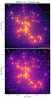 |
Fig. 3. Same as Fig. 2, but for the Hercules supercluster. |
| In the text | |
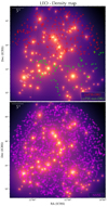 |
Fig. 4. Same as Fig. 2, but for the Leo supercluster. |
| In the text | |
|
Fig. 5. Total weighted RRM MAD variance (σMAD2RRM) trend with gas density in superclusters of galaxies. The plot shows the resulting variance from binning the sources in different gas density regimes. The background is divided into the ranges of densities that are typically related to voids (yellow), filaments (blue), and nodes (green; Cautun et al. 2014). The dashed red line represents where the gas ρ200 limit would approximately be, to highlight the density trend outside galaxy clusters. We measure an excess in the RRM variance between the first and second density bins, which can be attributed to the contribution of the low-density magnetised gas in the supercluster structure. Bottom panel: Same as the top panel, but varying the bins edges with steps of 0.03 (−0.03) with respect the original chosen value. The different resulting MAD variances and their uncertainties are show in different colours. The weighted average of these results in each bin is shown in blue and is consistent with the original value, shown in black. |
| In the text | |
|
Fig. 6. Posterior probability distribution, marginalised into one and two dimensions, for the parameters B||, L, and Λc. Dark and light blue shaded areas indicate the 68 and 95% confidence regions. The 1D projection for each parameters is shown at the top. The dashed blue lines represent (from left to right) the 2.5th, 50th, and 97.5th percentiles. |
| In the text | |
|
Fig. 7. Magnetic field marginalised posterior distribution, zoomed-in from Fig. 6. The distribution is skewed towards small values. The 95% confidence levels of the distribution are shown in dashed blue. The most likely value is shown in dashed red. The resulting adiabatic compression level is shown in purple. |
| In the text | |
|
Fig. 8. Covariance between the magnetic field strength (B||) and reversal scale (Λc), with the path length fixed to L = 70 Mpc. The distribution 1 and 2σ contour levels are shown in black. The dashed red line represent the magnetic field resulting from adiabatic compression only. |
| In the text | |
|
Fig. A.1. Absolute value of the Faraday spectrum (FDF; solid blue line) and the real (Q; solid green line) and imaginary (U; solid yellow line) components of the FDF, for two example polarised source components. The Q,U plots have a restricted range on the y-axis to better visualise the noise. The ‘real’ peak, i.e. the highest signal-to-noise polarised component outside the leakage range, is marked with a red cross. The leakage peak is noticeable in both cases at ϕ ∼ 0 rad m−2. The rms noise (σQU) level is shown as a dashed line. After inspection, the top source at S/N ∼ 8 is excluded, while the bottom source, at S/N ∼ 40 is accepted. |
| In the text | |
|
Fig. A.2. Inspection maps to evaluate the catalogued polarised source component. Top row: LoTSS 20″ resolution RM map, degree of polarisation map, and polarised intensity map for the catalogued source inside the Stokes I contours (black). Bottom row: FDF with the catalogued RM value and S/N for the peak, and the NVSS 45″ resolution Stokes I (black) and polarised intensity (green) contours for comparison. For the bottom source, the zoomed-in panel show the complexity of the spectrum around the selected peak. After inspection, the top source is accepted, while the bottom source is excluded. |
| In the text | |
Current usage metrics show cumulative count of Article Views (full-text article views including HTML views, PDF and ePub downloads, according to the available data) and Abstracts Views on Vision4Press platform.
Data correspond to usage on the plateform after 2015. The current usage metrics is available 48-96 hours after online publication and is updated daily on week days.
Initial download of the metrics may take a while.