| Issue |
A&A
Volume 693, January 2025
|
|
|---|---|---|
| Article Number | A208 | |
| Number of page(s) | 18 | |
| Section | Cosmology (including clusters of galaxies) | |
| DOI | https://doi.org/10.1051/0004-6361/202451333 | |
| Published online | 20 January 2025 | |
The nature of LOFAR rotation measures and new constraints on magnetic fields in cosmic filaments and on magnetogenesis scenarios
1
INAF – Istituto di Radioastronomia, Via Gobetti 101, 40129 Bologna, Italy
2
Dipartimento di Fisica e Astronomia, Universitá di Bologna, via Gobetti 93/2, 40122 Bologna, Italy
3
Hamburger Sternwarte, University of Hamburg, Gojenbergsweg 112, 21029 Hamburg, Germany
4
Departamento de Fisica de la Tierra y Astrofisica & IPARCOS-UCM, Universidad Complutense de Madrid, 28040 Madrid, Spain
5
INAF – Osservatorio Astronomico di Cagliari, Via della Scienza 5, 09047 Selargius (CA), Italy
6
ATNF, CSIRO Space & Astronomy, P.O. Box 1130 Bentley, WA 6102, Australia
7
SKA Observatory, SKA-Low Science Operations Centre, 26 Dick Perry Avenue, Kensington, WA 6151, Australia
8
Department of Space, Earth and Environment, Chalmers University of Technology, Onsala Space Observatory, 439 92 Onsala, Sweden
9
School of Natural Sciences and Medicine, Ilia State University, 3-5 Cholokashvili St., 0194 Tbilisi, Georgia
10
ICRAR, The University of Western Australia, 35 Stirling Hw, 6009 Crawley, Australia
⋆ Corresponding author; carretti@ira.inaf.it
Received:
1
July
2024
Accepted:
18
November
2024
The measurement of magnetic fields in cosmic web filaments can be used to reveal the magnetogenesis of the Universe. In previous works, we produced the first estimates of the field strength and its redshift evolution using the Faraday rotation measure (RM) catalogue of extragalactic background sources at a low frequency obtained with LOFAR observations. For this work, we refined our analysis by selecting sources with a low Galactic RM, which reduces its residual contamination. We also conducted a comprehensive analysis of the different contributions to the extragalactic RMs along the line of sight, and confirm that they are dominated by the cosmic filaments’ component, with only 21 percent originating in galaxy clusters and the circumgalactic medium (CGM) of galaxies. We find a possible hint of a shock at the virial radius of massive galaxies. We also find that the fractional polarisation of background sources might be a valuable CGM tracer. The newly selected RMs have a steeper evolution with redshift than previously found. The field strength in filaments (Bf) and its evolution were estimated assuming Bf evolves as a power law Bf = Bf, 0 (1 + z)α. Our analysis finds an average strength at z = 0 of Bf, 0 = 11–15 nG, with an error of 4 nG, and a slope α = 2.3–2.6 ± 0.5, which is steeper than what we previously found. The comoving field has a slope of β = [0.3, 0.6]±0.5 that is consistent with being invariant with redshift. Primordial magnetogenesis scenarios are favoured by our data, together with a sub-dominant astrophysical-origin RM component increasing with redshift.
Key words: magnetic fields / polarization / methods: statistical / intergalactic medium / large-scale structure of Universe
© The Authors 2025
 Open Access article, published by EDP Sciences, under the terms of the Creative Commons Attribution License (https://creativecommons.org/licenses/by/4.0), which permits unrestricted use, distribution, and reproduction in any medium, provided the original work is properly cited.
This article is published in open access under the Subscribe to Open model. Subscribe to A&A to support open access publication.
1. Introduction
The origin of the magnetic field of the Universe can be investigated through the evolution of several indirect proxies with cosmic time (e.g. Subramanian 2016; Vachaspati 2021; Arámburo-García et al. 2021; Vazza et al. 2021). The magnetic field in cosmic filaments is a sweet spot for such an investigation. There the field is not yet as processed as it is in galaxy clusters, where the memory of the initial conditions has been erased (Cho 2014; Vazza et al. 2017), keeping the information of the primeval conditions, whilst it is stronger than in voids, which makes the detection easier (Neronov & Vovk 2010; Vazza et al. 2017; Mtchedlidze et al. 2022). There are two major groups of magnetogenesis models: primordial scenarios, where the field was produced early, during cosmic inflation, or in phase transitions before recombination (e.g. Turner & Widrow 1988; Kronberg 1994; Paoletti & Finelli 2019), and astrophysical scenarios, where the magnetisation of the Universe was generated late in galaxies and active galactic nuclei (AGNs) and then injected in the intergalactic medium (IGM) (Kronberg 1994; Bertone et al. 2006; Donnert et al. 2009).
The Faraday rotation measure (RM) is a measure of the polarisation angle rotation by birifrangence of the two circular polarisation states, which is produced when polarised radiation travels through a magneto-ionic medium with a magnetic field and is populated with free electrons (a plasma). The RM depends on the magnetic field component along the line of sight (LOS), which is weighted by the electron number density and integrated along the LOS from the source to the observer. It is an effective tool to study magnetic fields and the ionised medium in the Galaxy (Planck Collaboration XLII 2016; Dickey et al. 2022), the circumgalactic medium (CGM) of galaxies (Heesen et al. 2023; Böckmann et al. 2023), the environment local to the source (Laing et al. 2008), and the cosmic web (Pomakov et al. 2022; Carretti et al. 2023; Vernstrom et al. 2023). It helps not only to investigate magnetic fields, but also to reveal the warm-hot intergalactic medium (WHIM) (Akahori & Ryu 2011; Anderson et al. 2021) that, with low temperatures of 104–106 K, is hard to detect in low density environments at other wavelengths (e.g. X-ray).
The evolution with redshift of the extragalactic RM was investigated in the past decades, mostly with no evolution being found (Fujimoto et al. 1971; Reinhardt 1972; Kronberg et al. 1977; Sofue et al. 1979; Kronberg & Perry 1982; Thomson & Nelson 1982; Welter et al. 1984; Oren & Wolfe 1995; You et al. 2003; Bernet et al. 2008; Vernstrom et al. 2018; Riseley et al. 2020). The extragalactic RMs at gigahertz frequencies are dominated by the contribution local to the source (Carretti et al. 2022). At these frequencies Fujimoto et al. (1971), Kronberg et al. (2008), and Lamee et al. (2016) found a hint of evolution using samples of up to a few hundreds of sources, which was attributed to the RM originating local to the source (Kronberg et al. 2008). However, this evolution was not confirmed using a much larger sample of ≈4000 sources (Hammond et al. 2012), and thus the results have been inconclusive so far.
Limits on the IGM magnetic field (i.e. the mean magnetic field strength of the Universe, averaged over all cosmic web structures such as voids, walls, and filaments) are set with several tracers. Rotation measures of extragalactic sources give an upper limit of 1.5 nG when measured at 144 MHz (Pomakov et al. 2022) and of 15 nG when measured at 1400 MHz (Vernstrom et al. 2019). The investigation of the synchrotron emission of the cosmic web has led to upper limits of 10–200 nG (Vernstrom et al. 2017; Brown et al. 2017). The temporal smearing distribution of fast radio bursts gives an upper limit of 10 nG (Padmanabhan & Loeb 2023). Delays in the arrival time of giga-electronvolt from tera-electronvolt γ-ray emission from blazars yield lower limits of 4 × 10⁻¹⁴ to 7 × 10⁻¹⁶ G in voids, depending on the blazar duty cycle (Aharonian et al. 2023). The time delays of lensed blazars give a lower limit of 2 × 10⁻¹⁷ G (Eroshenko 2024). Time delays of γ-rays from gamma ray bursts give lower limits of a few 10−19 G (e.g. Huang et al. 2023; Vovk et al. 2024). Using blazars, the filling factor of the IGM field has been constrained to f ≳ 0.67, which favours primordial over astrophysical models (Tjemsland et al. 2024).
The magnetic field in cosmic filaments has been measured at 30–60 nG using synchrotron emission stacking (Vernstrom et al. 2021) and at 40–80 nG with extragalactic RMs at low frequencies (Carretti et al. 2022, 2023). Vernstrom et al. (2023) find that filaments are highly polarised, which implies a significant ordered magnetic field component in filaments, consistent with the detection of an RM signal from them (Carretti et al. 2022). The high polarisation fraction also supports the theoretical paradigm of filament accretion with shocks from infalling matter. Carretti et al. (2023) estimated the evolution of the magnetic field strength with redshift. Their results are consistent with no evolution of the physical field out to z = 3. Upper limits were found by cross correlating the synchrotron emission at a low frequency with X-ray emission (Hoang et al. 2023), comparing synchrotron emission with simulations (Vacca et al. 2018), and cross-correlating RMs with cosmic web tracers (Amaral et al. 2021). Cosmic filaments have been recently detected in Lyman-α (Martin et al. 2023) and X-ray diffuse emission (Dietl et al. 2024). Magnetic fields have also been recently detected in the cosmic web just off galaxy groups (Anderson et al. 2024), where they have a strength of 200–600 nG and then drop under their dataset sensitivity at projected separations from groups beyond seven splashback radii.
In a previous work, we estimated the magnetic field strength in cosmic filaments using extragalactic source RMs at low frequencies of ≈144 MHz (Carretti et al. 2022, hereafter Paper I) and its evolution with redshift (Carretti et al. 2023, hereafter Paper II). We used the RM catalogue of O’Sullivan et al. (2023) derived from the LOFAR Two-metre Sky Survey (LoTSS; Shimwell et al. 2022) data. We also compared the RM–redshift evolution with that predicted by cosmological models, finding that primordial stochastic models are favoured. We find that the sight lines of polarised sources tend to avoid the high density environments of galaxy clusters at this low frequency, and that the RM of the extragalactic sources is dominated by that produced by the intervening cosmic filaments, with a minor contribution from the environment local to the source.
For this work we refined our analysis by improving our sample selection, specifically, only selecting sources with a low Galactic RM. We also conducted a comprehensive analysis of the different contributions to the extragalactic RMs we used, and again we find that once the Galactic RM is subtracted off, they are dominated by the IGM or cosmic web term. Finally, we estimated the strength and evolution with the redshift of the magnetic field in cosmic filaments, using a Bayesian analysis, and compared the results with the predictions of magnetogenesis models, including several new primordial stochastic ones, which our previous work found favoured compared to other magnetogenesis scenarios.
This paper is organised as follows. In Sect. 2 the RM sample at 144 MHz we used is described, and we explain how we computed the RM as a function of the redshift (z). Section 3 describes the magneto hydrodynamics (MHD) cosmological simulations used in this work. In Sect. 4 we investigate the origin of our RMs, specifically whether there is a significant contribution from intervening galaxy clusters, galaxies and their CGM, or the radio sources themselves. In Sect. 5 we explain how we fitted the strength and redshift evolution of the magnetic field in filaments to the observed extragalactic RM as a function of redshift. We also compare the observed RMs with those computed for a number of magnetogenesis scenarios. Finally, in Sect. 6 we discuss our results and draw our conclusions.
Throughout the paper we assume a flat ΛCDM cosmological model with H0 = 67.8 km s−1 Mpc−1, ΩM = 0.308, ΩΛ = 0.692, Ωb = 0.0468, and σ8 = 0.815 (Planck Collaboration XIII 2016). Errors refer to 1-σ uncertainties.
2. Faraday rotation measure data
2.1. LoTSS RM catalogue at 144 MHz
We use the RMs from the catalogue obtained from the LoTSS DR2 (LOFAR Two-metre Sky Survey Data Release 2) polarisation data (O’Sullivan et al. 2023; Shimwell et al. 2022). All details can be found in the paper describing the catalogue (O’Sullivan et al. 2023). Here we summarise the information relevant to this work. The observations were taken with the High Band Antenna (HBA) of the LOFAR telescope in a 48 MHz broad band centred at 144 MHz, with a frequency resolution of 97.6 kHz, and an angular resolution of 20 arcsec. The catalogue covers an area of 5720 deg2 and consists of 2461 RM components, 1949 of which have an associated redshift, either photometric or spectroscopic. The RMs are measured through RM-Synthesis (Burn 1966; Brentjens & de Bruyn 2005). The catalogue excludes the RM range of [−1, 3] rad m−2 to avoid sources possibly contaminated by instrumental polarisation leakage.
As done in Paper I and II, we filtered the sample by only keeping sources with a spectroscopic redshift (z) and at Galactic latitudes |b|> 25°, the latter is to avoid regions with large Galactic RM (GRM) contamination. This results in a sample of 1016 sources, the median and maximum redshift are 0.48 and 3.37.
The measured RMs are a combination of the GRM (more generally, the RM structures correlated on scales larger than ≈1°, which are dominated by the Milky Way ISM and its circumgalactic medium), the extragalactic RM (RMeg), and the noise (N):

The extragalactic term consists of an RM of astrophysical origin, either local to the source, mostly produced in the environment surrounding the source (Laing et al. 2008), or objects intervening along the sight line such as galaxy clusters or galaxies, and an RM generated in the cosmic web, mostly in filaments because the contribution from voids is marginal (see Paper II). The extragalactic term that we use in this work is estimated as the Residual RM:

At the low frequency of 144 MHz we work at, the astrophysical term is small (see Sect. 4) and the RRM is dominated by the cosmic filament term.
The GRM contribution to each source is estimated from the GRM map of Hutschenreuter et al. (2022) as the median of a disc of radius of 0.5° centred at the source to avoid a known bias at the source position (see Paper I and Hutschenreuter et al. 2022 for details). The radius of 0.5° is set to match the average separation of ≈1° between the sources used by Hutschenreuter et al. (2022) to derive their GRM map. The error is estimated by bootstrapping1. Blunier & Neronov (2024) have computed RRMs for the same LoTSS sample, estimating GRMs either with the same GRM map as used here or from Hutschenreuter & Enßlin (2020) and a method similar to ours. They obtain RRMs similar to ours with either map, which supports the robustness of our GRM estimate method.
The noise term consists of a measurement sensitivity term (Nm) and a GRM error (NGRM). The two noise terms quadratically add up in an RRM rms computation and they are subtracted off throughout the paper:

2.2. RRM rms versus GRM
The RRMs computed with Eq. (2) can still be affected by GRM estimate errors that are expected to be somewhat proportional to the GRM value. We thus filtered the sample for different GRM thresholds (GRMth), keeping sources with |GRM| < GRMth, and computed the RRM rms of each resulting sample. We excluded 2-σ outliers from the rms computation.
The result is shown in Fig. 1, left panel, that reports the RRM rms as a function of GRMth. The unfiltered sample, with a maximum |GRM| of 105.0 rad m−2, has an RRM rms of 1.90 ± 0.05 rad m−2. The minimum rms is at GRMth = 7 rad m−2 at 1.44 ± 0.07 rad m−2. Lower GRMth values do not give any reduction of the RRM rms and we infer that the residual GRM contributions are marginal, at the uncertainty level. However, this case with GRMth = 7 rad m−2 only includes 338 sources, a mere third of the full sample.
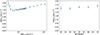 |
Fig. 1. RRM rms as a function of the GRM limit and Galactic latitude. Left: RRM rms of the spectroscopic redshift sample filtered by different GRM limits. The orange circle highlights the case with a limit of 14 rad m−2. Right: RRM rms as a function of Galactic latitude |b| for the case filtered with GRMth = 14 rad m−2. |
A more valuable option is the case with GRMth = 14 rad m−2. It gives an RRM rms of 1.54 ± 0.05 rad m−2, which differs from the minimum at some 1-σ confidence level (1.2-σ). It is still statistically consistent with the minimum, but it contains a much larger number of sources (653). The median GRM is 6.7 rad m−2. The median and maximum redshift of this sample are 0.47 and 3.22. Larger GRMth values return RRM rms values that differ from the minimum by more than 1.6-σ and we consider them not to be an option.
To check whether the GRMth = 14 rad m−2 case still retains a significant residual GRM contribution we computed the RRM rms in Galactic latitude |b| bins, of bin-width of Δ |b| = 10°. If a contribution is still present, a decrease of the RRM rms with |b| would be expected. Fig. 1, right panel, shows a rather flat behaviour with no obvious trend with |b|. The Spearman’s correlation rank of |RRM| as a function of |b| is ρ = −0.018 with a p-value of 0.64, which supports that RRM and b are uncorrelated in this sample.
To further check whether there is significant residual GRM contamination in our RRMs, we compute the RRM rms in |GRM| bins out to 14 rad m−2 (Fig. 2). Data with |GRM| < 3 rad m−2 are excluded to avoid the gap in RM that could produce an artificial correlaton. There is no obvious correlation, which is confirmed by a Spearman’s correlation rank of |RRM| versus |GRM| of ρ = 0.011 with an high p-value of p = 0.77. This supports a marginal residual GRM contamination.
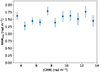 |
Fig. 2. RRM rms as a function of |GRM| of the spectroscopic redshift sample filtered by |GRM| < 14 rad m−2. |
Fig. 3 shows the RRM distribution of the same filtered sample. Compared to the RRM distribution of the unfiltered sample, also shown in Fig. 3. a reduction of the wings can be noticed.
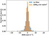 |
Fig. 3. RRM distribution of the spectroscopic redshift sample filtered by |GRM| < 14 rad m−2. The case with no GRM filter is also shown for comparison. |
These sanity checks are informative and necessary in order to assess to which extent can any strategy to separate Galactic and extragalactic contributions to the RMs of a sample of sources. Simpler procedures to remove the Galactic contribution can be biased (see the analysis in Paper I). This would result into a distribution of putative extragalactic RRMs that would instead show statistical correlations with the Galactic RM, signalling an incorrect estimate of the truly extragalactic component.
2.3. Behaviour of extragalactic RM with redshift
For the best fitting analysis of this work we use the spectroscopic redshift sample filtered for |GRM| < 14 rad m−2 discussed in Sect. 2.2. We computed the RRM rms in 20-source redshift bins (Fig. 4, left panel). The RRM rms is computed as for Eq. (3) and excluding 2-σ outliers. Errors are estimated by bootstrapping.
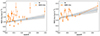 |
Fig. 4. RRM rms in redshift bins of 20 (left) and 40 (right) sources, each of the spectroscopic redshift sample filtered by |GRM| < 14 rad m−2. The linear fit (dashed line) and its uncertainty (shaded area) are also reported. |
Compared to the RRM rms of the full spectroscopic redshift sample (see Paper II), the RRM rms(z) of the GRM filtered sample computed here is steeper and lower, and at the z = 0 end it gets closer to 0. A weighted linear fit gives a slope of 0.25 ± 0.08 which is not flat at 3-σ significance.
We also show the plot of RRM rms as a function of redshift with 40-source bins (Fig. 4, right panel), which gives smaller errors. We note the presence of wiggles. We believe it is unlikely that they are related to the residual GRM contamination. They were also present in Paper II, where we used the full, unfiltered spectroscopic sample, and here, where we use a sample with reduced GRM contamination, they are still there. We discuss more on the wiggles in Sect. 4.2.
3. Cosmological MHD simulations
Compared to our previous work (Paper II), here we use a much improved set of cosmological magneto-hydrodynamical simulations produced using ENZO2, designed to investigate the dependence between RRM and different models of magnetogenesis with increased resolution and improved physical models.
We produced multiple resimulations of the same comoving volume of (42.5 Mpc)3 with a static grid of 10243 cells, giving a constant spatial resolution of 41.5 kpc/cell and a constant mass resolution of 1.01 × 10⁷ M⊙ per dark matter particle. Also based on our previous works, this volume was chosen to provide a reasonable compromise between a good spatial resolution in the medium or low density regions which are mostly contributing to the observed RRM (after the excision of denser halo regions), as well as a large enough cosmic volume to provide us a fair sampling of voids and filaments along simulated lines of sight. All runs include equilibrium gas cooling, a ‘sub-grid’ dynamo amplification model at run-time, which allows the estimation of the maximum contribution of a dynamo in low density environments (see Ryu et al. 2008), while the treatment of primordial magnetic fields and feedback from galaxy formation processes varies. In detail:
“Primordial uniform model”: a primordial uniform volume-filling comoving magnetic field strength of B0 = 0.1 nG initialised at the beginning of the simulation (z = 40).
“Primordial stochastic models”: three different initially tangled seed primordial magnetic fields, whose distribution of field scales follows a simple power law spectrum: PB(k) = PB0kαs characterised by a constant spectral index and an amplitude, commonly referred after smoothing the fields within a scale λ = 1 Mpc, using the same approach of Vazza et al. (2021). Here we simulated the αs = −1.0, = 0.0, = 1.0, and = 2.0 cases, that is, from very “red” to very “blue” primordial spectra, using the normalisation parameters given in Vazza et al. (2021) and based on observational constraints from the Cosmic Microwave Background obtained by Paoletti & Finelli (2019). “Red” spectra with a lower αs have most of their magnetic energy on the largest scales, mimicking the result of inflationary processes, while “blue” spectra with higher αs have more energy at smaller scales, with our limiting case here of αs = 2.0 which mimics the outcome of “causal” generation processes, in which the initial magnetic field is correlated only on scales smaller than the cosmological horizon. In detail, the adopted normalisation for each model is B1 Mpc = 0.003 nG for αs = 2.0, B1 Mpc = 0.042 nG for αs = 1.0, B1 Mpc = 0.35 nG for αs = 0.0 and B1 Mpc = 1.87 nG for the αs = −1.0. As will be discussed in Sect. 5.2, unlike in all other cases we found that downscaling the amplitude of the last, αs = −1.0 model, to B1 Mpc = 0.37 nG can produce a reasonable match to LOFAR RRMs.
“Astrophysical models”: two models in which magnetic fields were injected at run-time in the simulation, both by star forming particles and by simulated active galactic nuclei. In the first case, we used the star formation recipe by Kravtsov (2003), designed to reproduce the observed Kennicutt’s law (Kennicutt 1998) and with free parameters calibrated to reasonably reproduce the integrated star formation history and the stellar mass function of galaxies at z ≤ 2. The feedback from star forming particles assumes a fixed fraction of energy/momentum/mass ejected per each formed star particles, ESN = ϵSFm*c2, with efficiency calibrated to ϵSF = 10−8 as in previous work (Vazza et al. 2017). We also consider that 90% of the feedback energy is released in the thermal form (i.e. hot supernovae-driven winds), distributed to the 27 nearest cells around the star particle, and 10% in the form of magnetic energy, assigned to magnetic dipoles by each feedback burst.
The feedback from active galactic nuclei is treated by assuming that, at each timestep of the simulation, the highest density peaks in the simulation harbour a supermassive black hole, to which we assign a realistic mass based on observed scaling relations (e.g. Gaspari et al. 2019). We then compute the instantaneous mass growth rate onto each supermassive black hole by following the standard Bondi-Hoyle formalism, in which we include (as typically for simulations at this resolution) an ad hoc “boost” parameter meant to compensate for the lack of resolution around the Bondi radius. Depending on the temperature of the accreted gas, we use either “cold gas accretion” feedback (in which most of the energy is distributed in the form of thermal energy in the neighbourhood of each simulated AGN) or “hot gas accretion” feedback (in which most of the energy is released in the form of bipolar kinetic jets). In both cases, 10% of the feedback energy is released in the form of magnetic energy, through pairs of magnetised loops wrapped around the direction of kinetic jets. This magnetic field is added to a negligible uniform initial seed field of B0 = 10−11 nG (comoving), leading to “magnetic bubbles” correlated with halos in the simulated volume. The two variations studied in this work concerns two different set of parameters for the efficiency of feedback from the hot and cold gas accretion and are calibrated to well reproduce the radio luminosity functions of real radio galaxies in the local Universe, with the “astroph 2” model having an overall slightly more efficient feedback energetics, when integrated over the entire lifetime of the simulation. A more detailed descriptions of all parameters used in this model, as well as of the main comparison with simulated and observed galaxy properties is the subject of a forthcoming paper (Vazza et al. 2024).
“Mixed model”: we combined the astrophysical model giving the largest contribution to the magnetisation of the cosmic web of the two discussed above (“astroph 2”), and the stochastic primordial model that gives the best match to LOFAR RRMs (see Sect. 5.2), which is that with αs = −1.0 and downscaled normalisation B1 Mpc = 0.37 nG.
An overview of the numerical parameters of the tested magnetic fields in given in Table1. The adopted cosmological parameters are as for Sect. 1. The production of these new simulations was motivated in order to produce long lines-of-sight (LOS) with a finely sampled redshift evolution of gas and magnetic field quantities from z = 3 to z = 0, which was not available in existing simulations.
Parameters of the primordial magnetic fields tested in our suite of cosmological simulations.
To allow a comparison with the observed RM, we generated 100 LOS through each simulated volume, with information of gas density and 3D magnetic field from z = 2.98 to z = 0. Each LOS is ≈6.502 comoving Gpc long and was produced by replicating the simulated volume 153 times, using a set of 17 snapshots saved at nearly equally spaced redshifts, and by randomly varying the volume-to-volume crossing position. In total, for each simulated model we extracted 100 LOS, each containing physical field values for a total of 156 672 cells. Our analysis shows that the RRM integrated over such long LOS gives very stable trends, and already with a sample of 100 LOS the uncertainties on the RRM within each redshift bin are ≤0.1% (see Sect. 5.2).
4. Origin of RRM at low frequency
In Papers I and II we addressed the origin of the RRMs of our sample at 144 MHz. Analysing the evolution with redshift of the polarisation fraction p and the behaviour of RRM rms with p, we found that a cosmic web origin is favoured, as opposed to an astrophysical origin. We also estimated the separation of our sources and their LOS to galaxy clusters and found that they tend to be far from clusters. Thus, the source LOS tend to travel through low density environments, where the depolarisation is lower.
We also used the results of differential RMs of random pairs (sources with close projected separation, but not physically associated and at different redshifts) and physical pairs (sources physically associated at the same redshift, such as two lobes of a radio galaxy) by Pomakov et al. (2022) and found that a cosmic web contribution is dominant. The astrophysical origin term is estimated to be ≈10 percent.
All of the above points to an origin that is mostly from the cosmic web. The RRM from the cosmic web is largely dominated by the filament contribution because their RRM is much larger than that of voids, according to MHD cosmological simulations (Paper II). In this Section we further investigate the RRM origin at 144 MHz.
4.1. Galaxy clusters
We test whether the galaxy clusters can contribute to the RRMs we measure. If the RRMs are of cosmic origin it is expected that the RRM rms would be larger in lines of sight passing through a cluster, instead of solely through filaments and voids.
We first analyse the full spectroscopic redshift sample with no GRMth filter to investigate the origin of the RRMs used in our two previous papers.
For each RRM source we found the galaxy cluster with the smallest impact parameter (or projected separation from the source LOS) in R100 units3. We then computed the RRM rms as a function of this separation. We used the galaxy cluster catalogue of Wen & Han (2015). The catalogue contains 158 103 records in the redshift range of 0.05–0.75 with an error of up to 0.018. The cluster masses (M5004) are as low as 2.0 × 10¹² M⊙ and the catalogue is 95 percent complete for masses greater than 1.0 × 10¹⁴ M⊙. We selected sources of our RRM sample that are in the galaxy cluster catalogue redshift range, for a total of 707 sources. The RRM rms of this sample is 1.93 ± 0.06 rad m−2. We only used massive clusters (mass M > 1.0 × 10¹⁴ M⊙) that are expected to give the largest RRM effect. The rms is computed excluding 2-σ outliers5.
The rms as a function of separation is computed in bins of 0.45 R100 (which is approximately R500). Figure 5, top left panel, shows the RRM rms as a function of the minimum projected separation from clusters. We find an obvious excess of 6.8 ± 1.5 rad m−2 in the first bin (out to 0.45 R100), which contains 9 sources, whilst beyond 0.45 R100 there is no obvious trend, sitting at a mean value of 1.75 ± 0.06 rad m−2. The latter is 9 percent lower than the RRM rms of the entire sample and is an estimate of the astrophysical term contribution by intervening galaxy clusters to our RRM rms, for the full sample. It is important to note that the value of 6.8 rad m−2 is consistent with the rms of ≈7 rad m−2 of extragalactic sources observed at 1.4 GHz (e.g. Oppermann et al. 2015; Schnitzeler et al. 2019).
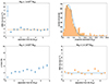 |
Fig. 5. RRM rms (top left), distribution (top right), and mean fractional polarisation (bottom left) of the full spectroscopic sample at 144 MHz in bins of the separation from the nearest galaxy cluster of mass M > 1.0 × 10¹⁴ M⊙ along the LOS. Bottom right: Same as the for the top left panel except it is for galaxy clusters of mass M < 1.0 × 10¹⁴ M⊙. |
Figure 5, bottom left panel, reports the mean polarisation fraction in the same bins. The first bin has a significantly low value of p = 0.62 ± 0.12 percent that is close to the limit of detection of our observations. The few sources whose LOS go through clusters at 144 MHz are thus highly depolarised and on the verge of not being detected. They are likely the few sources that survive such depolarisation and this can explain why so few are detected in polarisation. The polarisation fraction rises to ≈2 percent just beyond 0.45 R100 and then it increases nearly linearly with the separation. This increase might indicate that the environment density is decreasing with the separation to clusters leading to lower depolarisation. A small dip can be seen at ≈3 R100 ≈ 6 R500, the origin of which is still unclear.
Our result of high depolarisation of sources in the background of galaxy clusters is consistent with the results obtained at 1.4 GHz (Vacca et al. 2010; Bonafede et al. 2011; Osinga et al. 2022). However, while at 1.4 GHz high depolarisation is restricted to the inner regions of the cluster, here at low frequency it stretches out to the cluster outskirts, to ≈R500.
We checked whether there is a redshift dependence on how far out the depolarisation stretches. We split the sources in two redshift bins, lower and higher than 0.5, where we find 4 and 5 sources in the first bin. While the lower redshift bin has the depolarisation still limited to the first bin out to 0.45 R100, in the higher redshift bin (z = 0.5–0.75) the depolarisation stretches out to the second separation bin (Fig. 6), out to 0.9 R100 ≈ 2 R500, which is approximately the virial radius. That means that strong depolarisation effects are produced by the entire cluster. However, we verified that the RRM excess is still limited to the first separation bin.
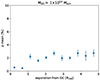 |
Fig. 6. Mean fractional polariation (p) at 144 MHz in bins of the impact parameter from the nearest galaxy cluster of mass M > 1.0 × 10¹⁴ M⊙ along the LOS. The case of the no GRM filter sample restricted to the redshift range z = 0.5–0.75 is shown. |
Figure 5, bottom right panel, shows the RRM rms when clusters of mass M < 1.0 × 10¹⁴ M⊙ are used, which comprises poor clusters and groups. No excess in the first bin out to 0.45 R100 shows up in such a case. The fractional polarisation p raises to 2.7 ± 0.7 percent. These results mean that groups and poor clusters give a marginal effect at this frequency.
The flat trend beyond 0.45 R100, as opposed to the excess within massive clusters, supports a cosmic web origin outside cluster environments. If the RRM rms depended on the local environment, then a decrease with the separation would be observed because of a decrease of density, while a dependence on all the cosmic filaments in the source foreground would result in a term uncorrelated with the separation from the cluster.
The source distribution as a function of the separation from clusters (x) (Fig. 5, top right panel) is well approximated by a Rayleigh distribution, which is the distribution of the magnitude of a 2D vector, as it is the projected separation on the plane of the sky:
where σr is the distribution spread and A is a normalisation term. The best fit (solid line) gives σr = 2.42 ± 0.05 R100. The cumulative distribution function is
We also measured the RRM rms as a function of the separation from galaxy clusters for the sample filtered by the GRMth limit of 14 rad m−2 (Fig. 7), which is the sample used for the analysis in this work. The RRM rms of the sources in the redshift range of the cluster catalogue is 1.56 ± 0.06 rad m−2. The RRM rms of the first bin is of 5.4 ± 2.8 rad m−2, which is consistent with that of the full sample case discussed above.
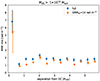 |
Fig. 7. RRM rms at 144 MHz in bins of the impact parameter from the nearest galaxy cluster of mass M > 1.0 × 10¹⁴ M⊙ along the LOS. The full spectroscopic redshift sample and an RRM sample filtered by a GRMth limit are shown. The cases are shifted in separation for clarity. |
The mean RRM rms excluding the first bin gets down to 1.26 ± 0.05 rad m−2. This is 19 ± 4 percent lower than that of the sample and can be considered as the fraction of the astrophysical RRM component from intervening clusters in the sample used in the analysis of this work.
It is worth noticing a hint of a secondary excess at ≈2 R100 ≈ 4R500 (2.1 σ and 2.4 σ significance for the no GRM filter and GRMth = 14 rad m−2 samples). This is possibly related to the presence of companion clusters, as previously found in the density and metallicity profiles obtained from simulations (Angelinelli et al. 2022, 2023). It is unlikely related to the source excess found close to the cluster virial radius (Ilani et al. 2024), which is closer than 2R100.
The mean p of the first bin is 0.77 ± 0.19 percent, again showing a small polarisation fraction as in the unfiltered sample. The Rayleigh distribution spread is similar to that of the no filter case, at σr = 2.51 ± 0.06 R100.
4.2. Galaxies and CGM
Here we analyse whether galaxies or their CGM give a contribution to the RRM sample we use in this work. This is motivated by the recent finding that nearby spiral galaxies can produce a measurable RRM excess at 144 MHz, if the LOS of a background extragalactic source goes through their extraplanar, magnetised outflows from the inner part of the galaxies close to their minor axis (Heesen et al. 2023). In such galaxies the excess RRM is detectable out to 100 kpc.
We analyse the RRM spectroscopic redshift sample with a GRMth filter set to 14 rad m−2.
For each RRM source we estimated the impact parameter of the LOS to the galaxy with the smallest impact parameter in kpc units, and then we computed the RRM rms as a function of that LOS separation. We considered the galaxy catalogue of6 Zou et al. (2019). The catalogue is based on the photometric survey Dark Energy Spectroscopic Instrument (DESI) Legacy Surveys and contains photometric redshifts and stellar masses (M*). It consists of approximately 3.03 × 10⁸ records with photometric redshifts up to z ≈ 1 and errors that depend mostly on their brightness. The median redshift errors for a few M* limited samples are reported in Table 2. The galaxy catalogue is complete for M* > 1011 M⊙ (see Fig. 12 of Zou et al. 2019). We selected sources of our RRM sample that are in the galaxy catalogue redshift range, a total of 550 sources. The RRM rms of such a subsample is 1.53 ± 0.05 rad m−2. We only used massive galaxies (stellar mass M∗ > 1011 M⊙) that are expected to give the largest effect. The main features of this subsample are reported in Table 2. The RRM rms is computed excluding outliers, as for Sect. 4.1.
The top panels of Fig. 8 show the RRM rms and the mean p as a function of the separation from galaxies in kiloparsecs. The bin size is 50 kpc. We do not observe any RRM excess in either the first bin out to 50 kpc nor in the second bin at 50–100 kpc. Also larger separations do not show any specific trend out to 1 Mpc. Our sample is not spiral galaxy-dominated, neither are the LOS selected to pass close to galaxy minor axis, thus our result of not finding any excess at short impact parameters is not inconsistent with the results of Heesen et al. (2023). The fractional polarisation is at about 2 percent in the first bins and then it slightly increases towards larger separations up to some 3 percent.
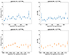 |
Fig. 8. RRM rms (top left) and ⟨p⟩ (top right) of the LoTSS RRM sample with a GRM limit of 14 rad m−2 versus source separation in kiloparsecs from galaxies of stellar mass M* > 1011 M⊙. The bin size is of 50 kpc. Bottom: as for top panels, except the separation is in virial radii, with bin size of 0.15 virial radii. |
The CGM extension depends on the halo mass (Mh) and redshift of the galaxy and these stacking plots mix different fractional separation within halos. Therefore, we also compute the same quantities in virial radius units (Fig. 8, bottom panels), that we expect to be more related to the CGM extension than the physical separation. For each galaxy, we estimate Mh from M* by the relation (Girelli et al. 2020)
![$$ \begin{aligned} M_* = 2M_h \, A(z)\left[ \left(\frac{M_h}{M_A(z)}\right)^{-\beta (z)} + \left(\frac{M_h}{M_A(z)}\right)^{\gamma (z)} \right]^{-1} \end{aligned} $$](/articles/aa/full_html/2025/01/aa51333-24/aa51333-24-eq6.gif)
where the best-fit parameters A, MA, β, and γ are listed in Table 1 of Girelli et al. (2020) as a function of redshift ranges. The virial radius is then estimated from rv = R100 (Reiprich et al. 2014) and using the equation
where ρc is the critical density of the Universe.
Again, there is no RRM excess closest to the galaxies. Intriguingly, the RRM tends to increase out to ≈0.8 rv. Further out, the RRM decreases to a mean value of 1.41 ± 0.06 rad m−2, which is 8 ± 5 percent lower than that of the sample. This can be considered an additional contribution of astrophysical origin. The RRM rms adds up quadratically, thus we can estimate the total astrophysical component contribution, intervening clusters and galaxies, at 21 ± 4 percent. The inner part of the RRM plot is difficult to interpret. On average, it sits about at the same value as the outer part. The first two bins are lower than average, while the two bins close to 0.8 rv are in excess. However, both the lower part and the excess are at low significance and might just be a statistical fluctuation. An intriguing possibility of the excess is as a signature of a shock at about the virial radius, perhaps infalling matter from the cosmic web surrounding the galaxy, or outflowing matter from the galaxy. Assuming plausible values of galaxy far outskirts for magnetic field (B = 0.1 μG), integration path (l = 50–200 kpc), and electron number density (ne = 10−4 cm−3), we get RRMs of 0.4–1.6 rad m−2 at z = 0 and 0.1–0.4 rad m−2 at z = 1, which are consistent with the excess we see here. We do not have plausible explanations for the first two lower bins, at this stage. Further investigations are required, with a larger sample for smaller errors and detailed modelling, especially of the smoothly decreasing RRM rms towards short separations. However, this is beyond the scope of this work.
The fractional polarisation is at ≈2 percent in the first bins, then it raises to 3–4 percent at ≈1.0 rv, where it flattens. The stronger depolarisation at shorter separations might be due to a turbulent medium in the CGM. We argue that ⟨p⟩ of background sources might be an efficient way to trace the CGM and its extension. However, further investigations are required to confirm this.
We estimate the RRM rms and ⟨p⟩ as a function of the separation from galaxies in rv units for two other galaxy subsamples, with M* = 1010–1011 M⊙ and M* = 109–1010 M⊙ (Fig. 9 and Table 2). These RRM profiles do not show the trend at separations within rv of the most massive subsample. The only possible feature is a hint of an excess (≈2.5 σ) at a separation of ≈0.25 rv in the M* = 109–1010 M⊙ subsample. With the caveat it has low significance, this excess might have a different origin compared to that found by Heesen et al. (2023) who do not find any excess in low mass galaxies.
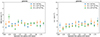 |
Fig. 9. RRM rms (left) and ⟨p⟩ (right) of the LoTSS RRM sample with a GRM limit of 14 rad m−2 versus LOS projected separation in virial radii from galaxies of the three samples of stellar mass M* > 1011 M⊙, M* = 1010–1011 M⊙, and M* = 109–1010 M⊙. The bin size is of 0.15 virial radii. |
As for the M* > 1011 M⊙ case, the mean p raises from the shortest separations and then it flattens out for the M* = 1010–1011 M⊙ subsample. We can see no obvious trend for the M* = 109–1010 M⊙ subsample.
We repeated the analysis flagging the galaxies with redshift error higher than either 3 times or 2 times the median error, to avoid sources with too large uncertainties, and we obtained the same results.
We also used our same galaxy sample limited to galaxies with M* > 1011 M⊙ to investigate possible correlations with the RRM wiggles of Fig. 4, right panel, that approximately peak at redshift of 0.15, 0.36, and 0.56. The galaxy number density as a function of redshift is shown in Fig. 10. There are three dips at redshifts of 0.125, 0.375, and 0.575 (with an uncertainty of 0.25, half the bin size), that well match the positions of the wiggles. The wiggles are interleaved by peaks of the galaxy number density, approximately matching the local minima of RRM rms vs redshift (Fig. 4). The first minimum of RRM rms, at z ≈ 0, corresponds to a raise of the number density. Thus, there is an anti-correlation. A RRM component of local origin is unlikely, because of the lower source density at the wiggles peaks. We do not have an obvious explanation for such a fascinating behaviour and further investigations will be needed.
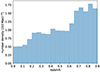 |
Fig. 10. Galaxy number density as a function of the redshift from the sample of galaxies with M* > 1011 M⊙ obtained from the DESI Legacy Surveys’ photometric galaxy catalogue. |
4.3. Dependence of RRM on the source spectral index
The spectral index of radio sources can discriminate radio galaxies from blazars, steeper and flatter, respectively, and can also depend on the local environment (e.g. Liu & Pooley 1991). The RRM is expected to be higher for more depolarised sources and hence to be stronger for blazars and for the more distant lobe of a radio galaxy (Laing 1988; Garrington et al. 1988). We thus would expect the RRM to have a dependence on the spectral index in case that our RRMs at low frequency would have a significant local component.
We explored the dependence of RRM on the spectral index of sources to assess whether there is a local origin. We used the spectral indexes measured by de Gasperin et al. (2018), who employed data from the TIFR GMRT Sky Survey (TGSS) at 147 MHz (Intema et al. 2017) and the NRAO VLA Sky Survey (NVSS) at 1.4 GHz (Condon et al. 1998).
We cross-matched the spectral index catalogue with the position of our sample of polarised sources with no GRM filter. We used a maximum separation of 22 arcsec, because the NVSS beam-size is 45 arcsec and Stokes I and polarised emission could be offset, finding a cross-match for 576 sources7.
Figure 11, top panel, reports RRM rms versus spectral index in bins of 0.2. Outliers beyond 2-σ are flagged. The bottom panel shows the source distribution with the spectral index. There is no obvious trend, looking flat within the errors. We checked three other cases: setting no maximum separation of the cross-match, thus using all sources of the original RM catalogue; setting a maximum separation of 7 arcsec for a safer cross-match; an RRM sample with a |GRM| limit of 14 rad m−2. In all cases, we obtain similar results.
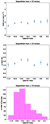 |
Fig. 11. RRM rms of the LoTSS RRM sample as a function of the spectral index obtained as described in the main text (top), polarisation fraction (mid), and spectral index distribution of the sources we used for this analysis (bottom). We used bins of a width of 0.2. |
The mean fractional polarisation also shows no obvious trend (Fig. 11, mid panel).
4.4. Dependence of RRM on the source linear size
We also checked for a dependence of the RRM rms on the source linear size. The linear size information is contained in the LoTSS RM catalogue for 725 sources of our unfiltered, spectroscopic redshift sample. Figure 12, top and bottom panels, show the RRM rms as a function of the source linear size and the corresponding distribution. Outliers beyond 2-σ are flagged. The RRM rms behaviour is flat.
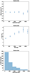 |
Fig. 12. RRM rms of the LoTSS RRM sample versus source linear size (top), mean fractional polarisation (mid), and linear size distribution of the sources we used for this analysis (bottom). We used bins of a width of 400 kpc. |
The mean fractional polarisation increases with the linear size (Fig. 12, mid panel). Giant radio galaxies, with sizes larger than 700 kpc, have the largest values. This is possibly because the largest radio galaxies have a higher chance to exit the densest regions of their local environment and the filaments spines, and are thus affected by smaller amounts of depolarisation.
We also tested the RRM sample limited to |GRM| < 14 rad m−2, obtaining similar results.
The lack of correlation of the RRM rms with source linear size and spectral index (Sect. 4.3) indicates the absence of a clear dependence of the total RRM on source properties. This again points to our RRMs being dominated by the non-local, cosmic web component.
5. Results
5.1. Strength and evolution with redshift of filament magnetic fields
Following the approach of Paper II, we estimate the average strength of the magnetic field in filaments and its evolution with redshift by Bayesian fitting of a model of the RRM rms to that measured with our RRM sample filtered by GRMth = 14 rad m−2. The RRM rms model is assumed to be (see Paper II):
where ne [cm−3] is the electron number density, B∥ [μG] is the magnetic field parallel to the LOS, and dl [pc] is the differential path length. All units are physical (proper) units. The term RRMf is the cosmic filament component and is computed for each of the 100 LOS we extracted from each magnetogenesis scenario. The term Arrm/(1 + z)2 accounts for an astrophysical component constant with redshift, either local or by intervening objects.
The gas density is taken from the LOS extracted from the MHD cosmological simulations. We only consider positions along the LOS where the gas contrast density (δg = ρg/⟨ρg⟩, with ρg the gas density) is greater than 1, which is a typical value to separate filaments from voids and because the underdensities give a negligible contribution to the RRM of the IGM (see Paper II).
As discussed in Paper II, and here in Sect. 4, the LOS of our polarised sources at low frequency tend to avoid galaxy clusters. To account for this, in Paper II we set a density contrast limit above which all LOS points were flagged. However, this does not account for the few sight lines that approach clusters with an impact parameter closer than R500 and that can contribute to the astrophysical component. Here we implement a procedure a little more sophisticated to mimic that the sources have different projected separations from clusters:
-
We search for the matter density maxima in each LOS and select those with matter density contrast above that at the cluster virial radius, which is ρM/ρc ≈ 50 or ρM/⟨ρM⟩≈160, where ρM is the density of the matter and ρc is the critical density of the Universe;
-
For each maximum, we draw a separation (x) from the distribution of Eqs. (4) and (5), setting σr = 2.51 R100 of the GRMth = 14 rad m−2 sample. Then we find the corresponding gas density contrast (δg, th) at that separation from a cluster (see Appendix A);
-
All pixels of the LOS with gas density contrast greater than δg, th and within a distance from the peak of 3 cMpc (comoving), are flagged and excluded from the RRM computation. The limit of 3 cMpc allows including clusters of any mass.
The strength of the proper magnetic field in filaments is assumed to follow the power law:

where Bf, 0 is the strength at z = 0. The comoving field follows the power law:
where8

The field direction is set randomly and changes each time the LOS enters a new filament, that is wherever δg is above 1. To increase the statistics, we produce 120 realisation of the field directions for each LOS. Thus, there are 12 000 RRMf realisations for each cosmological model, 100 LOS times 120 field realisations.
For each realisation we compute the RRMf as a function of z assuming a single value of Bf, 0. The slope α is set in the range of [−5, 5], spaced by 0.5. For each value of α, the RRMf rms is computed with the 12 000 realisations, 2-σ outliers are excluded. RRMf are smoothed on a scale Δz = 0.1. RRMf have a linear dependence on Bf, 0. The RRMf for a generic value of α is obtained by linearly interpolating the two closest values of α that the RRMf have been computed for. This gives the functional dependence on the two parameters that a Bayesian fitting needs.
Our Bayesian fit is a three-free-parameter fit that we conduct with the package EMCEE9 (Foreman-Mackey et al. 2013). We set priors of Bf, 0 < 250 nG (Locatelli et al. 2021), Bf, 0 ≧ 0, and Arrm ≧ 0. Best-fit results for all magnetogenesis scenarios considered here are reported in Table 3 and the fit plots for an example case, primordial stochastic model with spectrum slope of αs = 0.0, are shown in Fig. 13. The magnetic field strength at z = 0 is in the range Bf, 0 = 20–27 ± 5 nG, which is the range of results for the different magnetogenesis models and the typical statistical error. The slope of the physical magnetic field is in the range α = 1.7–2.1 ± 0.4. The field strength thus increases at a rate consistent with a comoving field invariant with redshift, the comoving slope being β = [ − 0.3, 0.1]±0.4. This is steeper than the behaviour found in Paper II and it comes from the steeper RRM rms versus redshift of the RRM sample we use here. The term Arrm is in the range 1.02–1.14 ± 0.11 rad m−2.
Best-fit parameters of the filament magnetic field strength and evolution with redshift to the measured RRM rms at 144-MHz of the sample filtered with GRMth = 14 rad m−2 and in case of an astrophysical component term of shape Arrm/(1 + z)2.
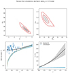 |
Fig. 13. Best-fit results of equation (8) to the RRM rms as a function of the redshift computed from the GRM filtered sample. The gas density is taken from the LOS extracted from the MHD simulation of the primordial stochastic model with αs = 0.0. The case with Bf independent of δg is assumed here. Top-left and top-right: 2D distributions (dots), and 1-sigma and 2-sigma confidence level contours (solid lines) of the fit parameters α, Bf, 0, and Arrm. Bottom-left: RRM rms measured in redshift bins (circles) and best-fit curve (solid) and its error range (grey-shaded area). The fit component of the sole filaments is also shown (dashed line) along with its uncertainty (shaded area). Bottom-right: Evolution with redshift z of the best-fit filament physical (solid line) and comoving magnetic field strength (dashed). The error range is also shown (shaded areas). |
We fitted Eq. (8) also using two other shapes of the astrophysical term instead of Arrm/(1 + z)2: (1) a cubed inverse dependence on redshift Arrm/(1 + z)3, which implies that the astrophysical RRM decreases with redshift as (1 + z)−1, and (2) an inverse dependence Arrm/(1 + z), which implies that the astrophysical RRM increases with redshift as (1 + z). The results are reported in the Tables 4 and 5. They are similar, consistent within the errors, to the previous case with: (1) Bf, 0 = 28–40 ± 7 nG, α = 1.2–1.6 ± 0.4, and Arrm = 1.04–1.20 ± 0.13 rad m−2, the strength is higher and the slope shallower compared to the standard case, possibly because of the degeneracy between these two quantities; (2) Bf, 0 = 11–15 ± 4 nG, α = 2.3–2.6 ± 0.5, and Arrm = 1.01–1.08 ± 0.09 rad m−2, the strength is smaller and the slope steeper.
The term Arrm/(1 + z)2 of Eq. (8) is meant to account for the local or intervening astrophysical objects component. Arrm is in the range 1.02–1.14 ± 0.11 rad m−2. If we assign to each source a contribution according to its redshift, the RRM rms because of the Arrm/(1 + z)2 term is 0.56–0.60 ± 0.06 rad m−2. Compared to the total rms of 1.54 ± 0.05 rad m−2, this corresponds to a fraction of 35–39 ± 4 percent, which is larger than the 21 ± 4 percent we estimated from clusters and CGM. The reasons we can identify are multiple: we are still missing an additional astrophysical component that contributes an additional ≈15 percent, either local or intervening; the astrophysical RM is not constant with redshift, as we assumed, and the corresponding astrophysical term does not depend on (1 + z)−2; a statistical difference (there is a tension at 2–3-σ). To start investigating the second of these options, we fit with different shapes of the astrophysical component term. The case with an astrophysical term decreasing with redshift, Arrm/(1 + z)3, gives an RRM rms contribution of 0.44–0.51 ± 0.06 rad m−2. This is a fraction of 29–33 ± 4 percent, which is closer to the observed 21 ± 4 percent than the previous, invariant with redshift case. The case with an astrophysical RRM increasing with redshift, Arrm/(1 + z), gives a fraction of 46–49 ± 4 percent, even larger than the invariant case. Even though the decreasing astrophysical term RRM shape is closest to the observed value, all shapes are in some tension.
In the previous fitting we assumed B as constant with the gas density. We perform a second series of fits using a model of the filament field where B ∝ ρg2/3, which corresponds to a magnetic field frozen to the plasma, a legitimate condition in the low density environment of filaments:
where  is the field strength at z = 0 and a gas density contrast of δg = 10, which is the typical value for cosmic filaments.
The results of the Bayesian fitting are reported in Table B.1 of Appendix B. We fitted the case with astrophysical component case of Arrm/(1 + z)2, which is mid way of the three shapes we tested. The ranges of the values are larger than in the previous fit, possibly because the computed RRMs now depend on ρg5/3. The field strength at δg = 10 and z = 0 ranges in  –10 ± 2 nG The slope sits at α = 2.0–2.7 ± 0.7. The slope of the comoving field ranges in β = [0.0, 0.7]±0.7.
5.2. RRM of filaments from cosmological simulations
Here we compute the RRMf rms of filaments of the magnetogenesis scenarios as a function of redshift using the magnetic field distributions directly produced by the cosmological MHD simulations. For each scenario, we computed the RRM versus redshift for each of the 100 LOS and then computed the rms. To account for the LOFAR polarised sources sight lines avoiding clusters, we apply the same procedure defined in Sect. 5.1 to flag points at high density contrast. The results are shown in Fig. 14. The RRM rms measured from our sample in 40-source bins is also reported for comparison. The latter has either the term Arrm/(1 + z) (left panel) or Arrm/(1 + z)3 (right panel) subtracted off to only display the cosmic filament component. The term Arrm is set to 1.08 rad m−2 and 1.20 rad m−2, respectively, that are the top of the ranges of the corresponding sets of fittings. We also show the corresponding filament component of the best fit.
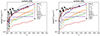 |
Fig. 14. Filaments’ RRMf rms as a function of the redshift of the cosmological models used in this work. The RRMs are computed using the gas densities and magnetic fields from the MHD cosmological simulations (astroph and astroph 2 are the first and second astrophysical models discussed in Sect. 3). The error bars of the simulated LOS are reported, albeit smaller than the markers (the typical mean fractional error is 0.07 percent). The measured RRM rms is also shown for comparison, with the Arrm/(1 + z) (left panel) or Arrm/(1 + z)3 (right panel) term subtracted off to only display the filament component. The corresponding filament component of the best fit is also shown (red, thick, dashed line) along with its uncertainty (shaded area). |
The comparison of the two panels of Fig. 14 shows a better match between the observed data and the simulations for the model with astrophysical RRM increasing with redshift, that is the shape Arrm/(1 + z), especially at low redshift.
A common feature of all primordial scenarios, either uniform or stochastic, is that their large filling factor for magnetic fields produce significant RRM already at high redshift, and their RRM rms show some slope. Their amplitude mostly depends on the initial normalisation. The astrophysical models produce cosmic fields late, injected by outflows and AGNs activity with a maximum at z ∼ 2, and have little power at high redshift. Their RRMf rms flattens and does not match the slope of the observed data.
At low redshift both the astrophysical models and the primordial models with highest power match the filament component of the fit to the observed data.
The slope of the observed RRM rms thus tends to favour primordial scenarios at high redshift. The stochastic models with αs ≥ 0 show RRM rms smaller than that measured already with the current normalisation, which is the highest consistent with CMB data (Paoletti & Finelli 2019; Paoletti et al. 2019), and look disfavoured by our sample. The model with αs = −1.0 and a normalisation that is 20 percent of the current limit from CMB data (i.e. 0.37 nG compared to the upper limit of 1.87 nG inferred by CMB modelling), looks to match the observed RRM rms. Its RRMf rms, also seems to match the observed data at low redshift. These considerations differ from the Paper II results, where the unfiltered sample gave an RRM rms flat at high redshift. We further elaborate on these differences in Sect. 6.
6. Discussion and conclusions
6.1. Origin of the RRM at low frequency
We have investigated possible correlations of the RRMs measured with LOFAR at 144 MHz with astrophysical sources to check whether their origin is the IGM or due to astrophysical sources.
We measured the RRM rms as a function of the projected separation of the source sight line from intervening galaxy clusters. We found an obvious excess at separations shorter than R500 for clusters of mass M > 1014 M⊙. This excess contributes for 19 percent to the total RRM rms. These are few sources (less than 2 percent) the polarisation fraction of which, some 0.6 percent, is much smaller than that of the bulk of the sources and close to the LoTSS detection limit. The sources whose sight lines pass through clusters are thus highly depolarised and only few of them survive complete depolarisation. At redshift beyond 0.5 the strong depolarisation stretches out to ≈R100. No obvious RRM excess is found beyond R500, which supports an IGM origin. The only exception is a possible small excess at a separation from cluster centres of some 2R100 ≈ 4R500, which might be associated to companion clusters typically found at that separation from rich clusters. We also find that the polarisation fraction increases with the separation from clusters, which indicates the density of the filament environment decreases with the separation from the cluster. We find no obvious excess for poor clusters and galaxy groups of mass M < 1014 M⊙, which indicates that only rich clusters can leave an RRM signature at this low frequency.
A similar analysis of the RRM rms as a function of the projected separation from massive galaxies (M* > 1011 M⊙) finds a possible hint of a shock in the CGM at the galaxy virial radius, which could possibly be produced by matter infalling from the cosmic web or outflows from the galaxies. This is small at some 0.5 rad m−2, and further investigations with larger RM samples or at higher frequencies are required to confirm it. POSSUM (Gaensler et al. 2010) or APERTIF (Adebahr et al. 2022) are well suited for conducting such an analysis. The RRM rms beyond the virial radius is 8 percent smaller than that of the entire sample, thus we find the galaxy CGM gives an additional contribution of astrophysical origin to the RRMs at this frequency. The polarisation fraction shows a clear, progressive decrement from the viral radius towards the galaxy centre and we argue the polarisation fraction of extragalactic background polarised sources can be a good tracer of the CGM. No obvious RRM trend is found for lower mass galaxies (M* < 1011 M⊙), as well as for the fractional polarisation of our lowest mass galaxy subsample (M* = 109–1010 M⊙).
A step forward in such an analysis can be done following Heesen et al. (2023) by only selecting star forming galaxies with large extraplanar outflows from the galaxy central regions. Also, the outflows orientation must be known, to select only cases where the LOS passes close to the galaxy minor axis and intercept the outflows. To our knowledge, such data are not yet available for the catalogue we use and such an analysis has to be postponed. The use of Mg II absorption lines in the sight lines of quasars can help identify galaxies with outflows (Bouché et al. 2007; Lundgren et al. 2012; Kacprzak et al. 2014; Schroetter et al. 2019) that have been suggested to harbor galaxy-scale extraplanar magnetic fields (Bernet et al. 2010; Joshi & Chand 2013; Farnes et al. 2014; Kim et al. 2016; Malik et al. 2020). This requires large spectroscopic datasets. A method as in Chang et al. (2015) can be used to separate star forming from quiescent galaxies. Overall, these are complex and extensive investigations that require their own dedicated work.
We also analysed the RRM rms as a function of source properties, such as size and spectral index, and we find no obvious correlation. This supports that the RRMs at this frequency have a marginal component of local origin. The polarisation fraction increases with the source size, which possibly is because larger sources extend beyond the centres of clusters and filament spines and are affected by lower depolarisation.
We thus conclude that the RRMs are dominated by the IGM/filaments component and only a contribution of ≈21 percent is of astrophysical object origin, that is galaxy clusters and galaxy CGM intervening along the source LOS. We note that the shape of the astrophysical contribution that better matches the RRM rms predicted by our MHD simulations implies that a further 25–30 percent of local origin might add up to the astrophysical contribution, but this is still uncertain. It is also worth noticing that, while the fractional polarisation is affected by local effects, the RRM rms is not, except when the depolarisation is high.
6.2. Magnetic fields in cosmic filaments
In this work we have filtered the LoTSS DR2 RMs, only selecting those with low GRM, to further reduce the residual GRM contamination after its subtraction. This produces a sample with an RRM rms ≈20 percent smaller than that of the unfiltered sample. There is negligible dependence of the RRM rms on the Galactic latitude and on GRM, which indicates little residual GRM contamination. The result is a smaller RRM rms which increases with redshift more steeply than in the original unfiltered sample.
The RRM rms as a function of redshift shows wiggles, the nature of which is still uncertain. They are unlikely to be due to GRM residuals. They are anti-correlated with the galaxy number density and thus unlikely are of local origin. Understanding their origin requires further investigation. They are associated with structures on scales of Δz ≈ 0.2, that is ≈800–900 Mpc. The wiggles thus are unlikely to appear in our MHD simulations whose boxes have a linear size of 42.5 Mpc.
Our model fitting of this sample finds a tension between the observed astrophysical component fractional contribution and that estimated from the fitting. The latter is larger by a factor of 1.5–2.5, depending on the shape of the term modelling the astrophysical component. We can identify a few possible causes of such a tension: (1) we are still missing an additional astrophysical component that contributes an additional ≈15 percent; (2) the astrophysical term has not the shapes we considered; (3) a statistical difference (it is at 2–4-σ). However, the data at low frequency are dominated by the IGM component and are not best to investigate the properties of the RRMs of astrophysical origin. This calls for RM data at higher frequency, that is dominated by the astrophysical component (see Paper I). Again, POSSUM and APERTIF can help in that.
The comparison of our data with the results of the MHD simulations of the magnetogenesis scenarios we consider in this work favours Arrm/(1 + z) as a shape for the astrophysical component term, which means that the RRM of astrophysical origin increases with redshift.
Assuming this astrophysical term, the best-fitting results are pretty independent of the magnetogenesis scenario used to draw the gas density. The average physical magnetic field strength in filaments at z = 0 is of Bf, 0 = 11–15 ± 4 nG. The slope as a function of (1 + z) is at α = 2.3–2.6 ± 0.5, while that of the comoving field is β = 0.3–0.6 ± 0.5, which is consistent with a comoving field invariant with redshift. This is steeper than our previous result of a physical field invariant with redshift and it comes from the steeper RRM versus redshift we found for this new GRM filtered sample.
The comparison with the RRM rms predicted by different magnetogenesis scenarios favours primordial models, either uniform or stochastic with a power spectrum slope of αs = −1.0. These models, having magnetic field power at high redshift, give an RRM rms increasing with redshift, as observed. Also at low redshift there is a good match with the observed data. The astrophysical scenarios produce magnetic fields late with little power at high redshift where their RRM rms flattens, inconsistent with the observations. A combined primordial and astrophysical model gives results similar to the primordial model and it is also favoured.
The amplitudes of the simulated primordial stochastic models look to be on the low side, i.e. even using the upper limits allowed by CMB constraints, the simulated RRM is significantly lower than the data. Only the α = −1.0 case, of those tested in this work, reproduces the LOFAR RRM data if an amplitude significantly smaller than the corresponding upper limits from the CMB is used. However, in this work we only simulated non-helical fields. Helical fields of primordial models may in principle produce a different pattern of RRMs (Mtchedlidze et al. 2022), as well as be subject to different constraints from CMB analysis. The power of the primordial uniform model is too high, but it can be fixed with a lower initial normalisation of the order of 0.05 nG.
Compared to the simulations used in Paper II, there are two main differences. First, the RRMs of the astrophysical models are higher, albeit smaller than the observed RRM by LOFAR. The increase in the magnetic output stems from the use of a 64 times finer mass resolution of the dark matter component and a 4 times better spatial resolution, giving better resolved star forming regions and galaxy evolution. This resulted in a larger fraction of low-mass halos (dwarf galaxies), which in turn has increased the magnetisation of voids and filaments and likely generated higher RRM even in the low density environments we explore in our analysis. Also, this model has been calibrated in more detail against both cosmic star formation history and the distribution of observable radio galaxies connected to the AGN model (Vazza et al. 2024). There are a couple of more items to be considered:
-
The basic result that a purely astrophysical origin scenario for extragalactic magnetic fields under predicts the amount of observed RRM at all redshift is consistent with Paper II and other works that reported incompatibility between this model and the non-detection of the Inverse Compton Cascade from blazars (Bondarenko et al. 2022; Tjemsland et al. 2024).
-
We must note that the level of the RRM predicted by other simulations is higher than what we predict here and in Paper II with our cosmological simulations (e.g. Arámburo-García et al. 2022, 2023; Blunier & Neronov 2024). This might signal that, despite how low the density where most of the RRM detected by LOFAR originates from, modern numerical simulations are not in agreement with their predictions in low-density environments, although they are able to reproduce the most basic properties of galaxy populations (e.g. stellar mass distribution and star formation history). This, in turn, strengthens the use of deep radio observations, like those used here, in giving strong constraints to feedback models applied to simulations of galaxy formation, in regimes which are otherwise very difficult to probe with other observational techniques.
The second significant difference with simulations in Paper II is the significantly smaller RRMs of the stochastic model with αs = 1. This is likely a resolution dependent effect. For the primordial models that have most of the power at small spatial scales, any change in resolution introduces more field reversals along the line of sight. The increased magnetic energy at small scales affects, both, the dynamics of gas already since the start of the simulation, as well as the small-scale distribution of magnetic fields at any epoch of the simulation. Combined with the removal of dense halos from this more resolved set of simulations, we think that this effect is plausibly responsible for a reduction of a factor ≈2 in the global RRM trend measured in this new set of simulations.
In summary, these trends call for future larger simulations, with even better resolution and detail on galaxy formation processes, and also including more realistic magnetic fields topologies (e.g. helicity) to seek a possible convergence of these RRMs on the density regime that is most relevant to compare with LOFAR observations.
We also would like to highlight that reducing the residual GRM contamination has significantly changed the redshift evolution scenario from flat to a significant evolution. Even if we have done an important work to minimise bias and residuals, this emphasises the need for even better GRM maps. A leap in this field can be obtained by POSSUM, thanks to both its high RM density and sensitivity.[10]https://lofar-mksp.org/[11]http://healpix.sf.net

We only used the sources of de Gasperin et al. (2018) with safer spectral index, that is the records with keyword S_code labelled as S or M.
Acknowledgments
We thank an anonymous referee for their thoughtful comments that allowed us to improve the paper. This work has been conducted within the LOFAR Magnetism Key Science Project10 (MKSP). This work has made use of LoTSS DR2 data (Shimwell et al. 2022). EC and VV acknowledge this work has been conducted within the INAF program METEORA. VV acknowledges support from the Premio per Giovani Ricercatori “Gianni Tofani” II edizione, promoted by INAF-Osservatorio Astrofisico di Arcetri (DD n. 84/2023). AB acknowledges support from ERC Stg DRANOEL n. 714245 and MIUR FARE grant “SMS”. SPO acknowledges support from the Comunidad de Madrid Atracción de Talento program via grant 2022-T1/TIC-23797, and grant PID2023-146372OB-I00 funded by MICIU/AEI/10.13039/501100011033 and by ERDF, EU. FV and SM have been supported by Fondazione Cariplo and Fondazione CDP, thorugh grant n° Rif: 2022-2088 CUP J33C22004310003 for “BREAKTHRU” project. In this work we used the ENZO code (http://enzo-project.org), the product of a collaborative effort of scientists at many universities and national laboratories. FV acknowledges the CINECA award “IsB28_RADGALEO” under the ISCRA initiative, for the availability of high-performance computing resources and support. LOFAR (van Haarlem et al. 2013) is the Low Frequency Array designed and constructed by ASTRON. It has observing, data processing, and data storage facilities in several countries, which are owned by various parties (each with their own funding sources), and which are collectively operated by the ILT foundation under a joint scientific policy. The ILT resources have benefited from the following recent major funding sources: CNRS-INSU, Observatoire de Paris and Université d’Orléans, France; BMBF, MIWF-NRW, MPG, Germany; Science Foundation Ireland (SFI), Department of Business, Enterprise and Innovation (DBEI), Ireland; NWO, The Netherlands; The Science and Technology Facilities Council, UK; Ministry of Science and Higher Education, Poland; The Istituto Nazionale di Astrofisica (INAF), Italy. LoTSS made use of the Dutch national e-infrastructure with support of the SURF Cooperative (e-infra 180169) and the LOFAR e-infra group. The Jülich LOFAR Long Term Archive and the German LOFAR network are both coordinated and operated by the Jülich Supercomputing Centre (JSC), and computing resources on the supercomputer JUWELS at JSC were provided by the Gauss Centre for Supercomputing e.V. (grant CHTB00) through the John von Neumann Institute for Computing (NIC). LoTSS made use of the University of Hertfordshire high-performance computing facility and the LOFAR-UK computing facility located at the University of Hertfordshire and supported by STFC [ST/P000096/1], and of the Italian LOFAR IT computing infrastructure supported and operated by INAF, and by the Physics Department of Turin university (under an agreement with Consorzio Interuniversitario per la Fisica Spaziale) at the C3S Supercomputing Centre, Italy. This work made use of the Python packages NumPy (Harris et al. 2020), Astropy (Astropy Collaboration 2013), Matplotlib (Hunter 2007), and EMCEE (Foreman-Mackey et al. 2013). Some of the results in this paper have been derived using the healpy (Zonca et al. 2019) and HEALPix11 (Górski et al. 2005) packages.
References
- Adebahr, B., Berger, A., Adams, E. A. K., et al. 2022, A&A, 663, A103 [NASA ADS] [CrossRef] [EDP Sciences] [Google Scholar]
- Aharonian, F., Aschersleben, J., Backes, M., et al. 2023, ApJ, 950, L16 [NASA ADS] [CrossRef] [Google Scholar]
- Akahori, T., & Ryu, D. 2011, ApJ, 738, 134 [NASA ADS] [CrossRef] [Google Scholar]
- Amaral, A. D., Vernstrom, T., & Gaensler, B. M. 2021, MNRAS, 503, 2913 [NASA ADS] [CrossRef] [Google Scholar]
- Anderson, C. S., Heald, G. H., Eilek, J. A., et al. 2021, PASA, 38 [Google Scholar]
- Anderson, C. S., McClure-Griffiths, N. M., Rudnick, L., et al. 2024, MNRAS, 533, 4068 [NASA ADS] [CrossRef] [Google Scholar]
- Angelinelli, M., Ettori, S., Dolag, K., Vazza, F., & Ragagnin, A. 2022, A&A, 663, L6 [NASA ADS] [CrossRef] [EDP Sciences] [Google Scholar]
- Angelinelli, M., Ettori, S., Dolag, K., Vazza, F., & Ragagnin, A. 2023, A&A, 675, A188 [NASA ADS] [CrossRef] [EDP Sciences] [Google Scholar]
- Arámburo-García, A., Bondarenko, K., Boyarsky, A., et al. 2021, MNRAS, 505, 5038 [NASA ADS] [CrossRef] [Google Scholar]
- Arámburo-García, A., Bondarenko, K., Boyarsky, A., et al. 2022, MNRAS, 515, 5673 [CrossRef] [Google Scholar]
- Arámburo-García, A., Bondarenko, K., Boyarsky, A., et al. 2023, MNRAS, 519, 4030 [CrossRef] [Google Scholar]
- Astropy Collaboration (Robitaille, T. P., et al.) 2013, A&A, 558, A33 [NASA ADS] [CrossRef] [EDP Sciences] [Google Scholar]
- Bernet, M. L., Miniati, F., Lilly, S. J., Kronberg, P. P., & Dessauges-Zavadsky, M. 2008, Nature, 454, 302 [NASA ADS] [CrossRef] [Google Scholar]
- Bernet, M. L., Miniati, F., & Lilly, S. J. 2010, ApJ, 711, 380 [NASA ADS] [CrossRef] [Google Scholar]
- Bertone, S., Vogt, C., & Enßlin, T. 2006, MNRAS, 370, 319 [NASA ADS] [Google Scholar]
- Blunier, J., & Neronov, A. 2024, A&A, 691, A34 [NASA ADS] [CrossRef] [EDP Sciences] [Google Scholar]
- Böckmann, K., Brüggen, M., Heesen, V., et al. 2023, A&A, 678, A56 [NASA ADS] [CrossRef] [EDP Sciences] [Google Scholar]
- Bonafede, A., Govoni, F., Feretti, L., et al. 2011, A&A, 530, A24 [CrossRef] [EDP Sciences] [Google Scholar]
- Bondarenko, K., Boyarsky, A., Korochkin, A., et al. 2022, A&A, 660, A80 [NASA ADS] [CrossRef] [EDP Sciences] [Google Scholar]
- Bouché, N., Murphy, M. T., Péroux, C., et al. 2007, ApJ, 669, L5 [CrossRef] [Google Scholar]
- Brentjens, M. A., & de Bruyn, A. G. 2005, A&A, 441, 1217 [NASA ADS] [CrossRef] [EDP Sciences] [Google Scholar]
- Brown, S., Vernstrom, T., Carretti, E., et al. 2017, MNRAS, 468, 4246 [NASA ADS] [CrossRef] [Google Scholar]
- Burn, B. J. 1966, MNRAS, 133, 67 [Google Scholar]
- Carretti, E., Vacca, V., O’Sullivan, S. P., et al. 2022, MNRAS, 512, 945 [NASA ADS] [CrossRef] [Google Scholar]
- Carretti, E., O’Sullivan, S. P., Vacca, V., et al. 2023, MNRAS, 518, 2273 [Google Scholar]
- Chang, Y.-Y., van der Wel, A., da Cunha, E., & Rix, H.-W. 2015, ApJS, 219, 8 [Google Scholar]
- Cho, J. 2014, ApJ, 797, 133 [NASA ADS] [CrossRef] [Google Scholar]
- Condon, J. J., Cotton, W. D., Greisen, E. W., et al. 1998, AJ, 115, 1693 [Google Scholar]
- de Gasperin, F., Intema, H. T., & Frail, D. A. 2018, MNRAS, 474, 5008 [Google Scholar]
- Dickey, J. M., West, J., Thomson, A. J. M., et al. 2022, ApJ, 940, 75 [NASA ADS] [CrossRef] [Google Scholar]
- Dietl, J., Pacaud, F., Reiprich, T. H., et al. 2024, A&A, 691, A286 [NASA ADS] [CrossRef] [EDP Sciences] [Google Scholar]
- Donnert, J., Dolag, K., Lesch, H., & Müller, E. 2009, MNRAS, 392, 1008 [NASA ADS] [CrossRef] [Google Scholar]
- Eroshenko, Y. N. 2024, Chin. Phys. C, 48, 015104 [NASA ADS] [CrossRef] [Google Scholar]
- Farnes, J. S., O’Sullivan, S. P., Corrigan, M. E., & Gaensler, B. M. 2014, ApJ, 795, 63 [NASA ADS] [CrossRef] [Google Scholar]
- Foreman-Mackey, D., Hogg, D. W., Lang, D., & Goodman, J. 2013, PASP, 125, 306 [Google Scholar]
- Fujimoto, M., Kawabata, K., & Sofue, Y. 1971, Prog. Theor. Phys. Suppl., 49, 181 [CrossRef] [Google Scholar]
- Gaensler, B. M., Landecker, T. L., Taylor, A. R., & POSSUM Collaboration 2010, Am. Astron. Soc. Meeting Abstr., 215, 47013 [Google Scholar]
- Garrington, S. T., Leahy, J. P., Conway, R. G., & Laing, R. A. 1988, Nature, 331, 147 [Google Scholar]
- Gaspari, M., Eckert, D., Ettori, S., et al. 2019, ApJ, 884, 169 [NASA ADS] [CrossRef] [Google Scholar]
- Girelli, G., Pozzetti, L., Bolzonella, M., et al. 2020, A&A, 634, A135 [NASA ADS] [CrossRef] [EDP Sciences] [Google Scholar]
- Górski, K. M., Hivon, E., Banday, A. J., et al. 2005, ApJ, 622, 759 [Google Scholar]
- Hammond, A. M., Robishaw, T., & Gaensler, B. M. 2012, arXiv e-prints [arXiv:1209.1438] [Google Scholar]
- Harris, C. R., Millman, K. J., van der Walt, S. J., et al. 2020, Nature, 585, 357 [NASA ADS] [CrossRef] [Google Scholar]
- Heesen, V., O’Sullivan, S. P., Brüggen, M., et al. 2023, A&A, 670, L23 [NASA ADS] [CrossRef] [EDP Sciences] [Google Scholar]
- Hoang, D. N., Brüggen, M., Zhang, X., et al. 2023, MNRAS, 523, 6320 [CrossRef] [Google Scholar]
- Huang, Y.-Y., Dai, C.-Y., Zhang, H.-M., Liu, R.-Y., & Wang, X.-Y. 2023, ApJ, 955, L10 [NASA ADS] [CrossRef] [Google Scholar]
- Hunter, J. D. 2007, Comput. Sci. Eng., 9, 90 [NASA ADS] [CrossRef] [Google Scholar]
- Hutschenreuter, S., & Enßlin, T. A. 2020, A&A, 633, A150 [EDP Sciences] [Google Scholar]
- Hutschenreuter, S., Anderson, C. S., Betti, S., et al. 2022, A&A, 657, A43 [NASA ADS] [CrossRef] [EDP Sciences] [Google Scholar]
- Ilani, G., Hou, K.-C., & Keshet, U. 2024, JCAP, 2024, 008 [CrossRef] [Google Scholar]
- Intema, H. T., Jagannathan, P., Mooley, K. P., & Frail, D. A. 2017, A&A, 598, A78 [NASA ADS] [CrossRef] [EDP Sciences] [Google Scholar]
- Joshi, R., & Chand, H. 2013, MNRAS, 434, 3566 [NASA ADS] [CrossRef] [Google Scholar]
- Kacprzak, G. G., Martin, C. L., Bouché, N., et al. 2014, ApJ, 792, L12 [NASA ADS] [CrossRef] [Google Scholar]
- Kennicutt, R. C., Jr 1998, ApJ, 498, 541 [Google Scholar]
- Kim, K. S., Lilly, S. J., Miniati, F., et al. 2016, ApJ, 829, 133 [NASA ADS] [CrossRef] [Google Scholar]
- Kravtsov, A. V. 2003, ApJ, 590, L1 [NASA ADS] [CrossRef] [Google Scholar]
- Kronberg, P. P. 1994, Rep. Prog. Phys., 57, 325 [NASA ADS] [CrossRef] [Google Scholar]
- Kronberg, P. P., & Perry, J. J. 1982, ApJ, 263, 518 [NASA ADS] [CrossRef] [Google Scholar]
- Kronberg, P. P., Reinhardt, M., & Simard-Normandin, M. 1977, A&A, 61, 771 [NASA ADS] [Google Scholar]
- Kronberg, P. P., Bernet, M. L., Miniati, F., et al. 2008, ApJ, 676, 70 [CrossRef] [Google Scholar]
- Laing, R. A. 1988, Nature, 331, 149 [Google Scholar]
- Laing, R. A., Bridle, A. H., Parma, P., & Murgia, M. 2008, MNRAS, 391, 521 [NASA ADS] [CrossRef] [Google Scholar]
- Lamee, M., Rudnick, L., Farnes, J. S., et al. 2016, ApJ, 829, 5 [NASA ADS] [CrossRef] [Google Scholar]
- Liu, R., & Pooley, G. 1991, MNRAS, 249, 343 [NASA ADS] [Google Scholar]
- Locatelli, N., Vazza, F., Bonafede, A., et al. 2021, A&A, 652, A80 [NASA ADS] [CrossRef] [EDP Sciences] [Google Scholar]
- Lundgren, B. F., Brammer, G., van Dokkum, P., et al. 2012, ApJ, 760, 49 [NASA ADS] [CrossRef] [Google Scholar]
- Malik, S., Chand, H., & Seshadri, T. R. 2020, ApJ, 890, 132 [NASA ADS] [CrossRef] [Google Scholar]
- Martin, D. C., Darvish, B., Lin, Z., et al. 2023, Nat. Astron., 7, 1390 [NASA ADS] [CrossRef] [Google Scholar]
- Mtchedlidze, S., Domínguez-Fernández, P., Du, X., et al. 2022, ApJ, 929, 127 [NASA ADS] [CrossRef] [Google Scholar]
- Neronov, A., & Vovk, I. 2010, Science, 328, 73 [NASA ADS] [CrossRef] [Google Scholar]
- Oppermann, N., Junklewitz, H., Greiner, M., et al. 2015, A&A, 575, A118 [NASA ADS] [CrossRef] [EDP Sciences] [Google Scholar]
- Oren, A. L., & Wolfe, A. M. 1995, ApJ, 445, 624 [NASA ADS] [CrossRef] [Google Scholar]
- Osinga, E., van Weeren, R. J., Andrade-Santos, F., et al. 2022, A&A, 665, A71 [NASA ADS] [CrossRef] [EDP Sciences] [Google Scholar]
- O’Sullivan, S. P., Shimwell, T. W., Hardcastle, M. J., et al. 2023, MNRAS, 519, 5723 [CrossRef] [Google Scholar]
- Padmanabhan, H., & Loeb, A. 2023, ApJ, 946, L18 [CrossRef] [Google Scholar]
- Paoletti, D., & Finelli, F. 2019, JCAP, 2019, 028 [CrossRef] [Google Scholar]
- Paoletti, D., Chluba, J., Finelli, F., & Rubiño-Martín, J. A. 2019, MNRAS, 484, 185 [NASA ADS] [CrossRef] [Google Scholar]
- Planck Collaboration XIII. 2016, A&A, 594, A13 [NASA ADS] [CrossRef] [EDP Sciences] [Google Scholar]
- Planck Collaboration XLII. 2016, A&A, 596, A103 [NASA ADS] [CrossRef] [EDP Sciences] [Google Scholar]
- Pomakov, V. P., O’Sullivan, S. P., Brüggen, M., et al. 2022, MNRAS, 515, 256 [NASA ADS] [CrossRef] [Google Scholar]
- Reinhardt, M. 1972, A&A, 19, 104 [NASA ADS] [Google Scholar]
- Reiprich, T. H., Basu, K., Ettori, S., et al. 2014, in Suzaku-MAXI 2014: Expanding the Frontiers of the X-ray Universe, eds. M. Ishida, R. Petre, & K. Mitsuda, 362 [Google Scholar]
- Riseley, C. J., Galvin, T. J., Sobey, C., et al. 2020, PASA, 37, e029 [Google Scholar]
- Roncarelli, M., Ettori, S., Dolag, K., et al. 2006, MNRAS, 373, 1339 [Google Scholar]
- Ryu, D., Kang, H., Cho, J., & Das, S. 2008, Science, 320, 909 [NASA ADS] [CrossRef] [Google Scholar]
- Schnitzeler, D. H. F. M., Carretti, E., Wieringa, M. H., et al. 2019, MNRAS, 485, 1293 [NASA ADS] [CrossRef] [Google Scholar]
- Schroetter, I., Bouché, N. F., Zabl, J., et al. 2019, MNRAS, 490, 4368 [CrossRef] [Google Scholar]
- Shimwell, T. W., Hardcastle, M. J., Tasse, C., et al. 2022, A&A, 659, A1 [NASA ADS] [CrossRef] [EDP Sciences] [Google Scholar]
- Sofue, Y., Fujimoto, M., & Kawabata, K. 1979, PASJ, 31, 125 [NASA ADS] [Google Scholar]
- Subramanian, K. 2016, Rep. Prog. Phys., 79, 076901 [NASA ADS] [CrossRef] [Google Scholar]
- Thomson, R. C., & Nelson, A. H. 1982, MNRAS, 201, 365 [NASA ADS] [CrossRef] [Google Scholar]
- Tjemsland, J., Meyer, M., & Vazza, F. 2024, ApJ, 963, 135 [NASA ADS] [CrossRef] [Google Scholar]
- Turner, M. S., & Widrow, L. M. 1988, Phys. Rev. D, 37, 2743 [NASA ADS] [CrossRef] [Google Scholar]
- Vacca, V., Murgia, M., Govoni, F., et al. 2010, A&A, 514, A71 [CrossRef] [EDP Sciences] [Google Scholar]
- Vacca, V., Murgia, M., Govoni, F., et al. 2018, MNRAS, 479, 776 [CrossRef] [Google Scholar]
- Vachaspati, T. 2021, Rep. Prog. Phys., 84, 074901 [NASA ADS] [CrossRef] [Google Scholar]
- van Haarlem, M. P., Wise, M. W., Gunst, A. W., et al. 2013, A&A, 556, A2 [NASA ADS] [CrossRef] [EDP Sciences] [Google Scholar]
- Vazza, F., Brüggen, M., Gheller, C., et al. 2017, CQG, 34, 234001 [NASA ADS] [CrossRef] [Google Scholar]
- Vazza, F., Paoletti, D., Banfi, S., et al. 2021, MNRAS, 500, 5350 [Google Scholar]
- Vazza, F., Gheller, C., Zanetti, F., et al. 2024, A&A, submitted [Google Scholar]
- Vernstrom, T., Gaensler, B. M., Brown, S., Lenc, E., & Norris, R. P. 2017, MNRAS, 467, 4914 [NASA ADS] [CrossRef] [Google Scholar]
- Vernstrom, T., Gaensler, B. M., Vacca, V., et al. 2018, MNRAS, 475, 1736 [NASA ADS] [CrossRef] [Google Scholar]
- Vernstrom, T., Gaensler, B. M., Rudnick, L., & Andernach, H. 2019, ApJ, 878, 92 [NASA ADS] [CrossRef] [Google Scholar]
- Vernstrom, T., Heald, G., Vazza, F., et al. 2021, MNRAS, 505, 4178 [NASA ADS] [CrossRef] [Google Scholar]
- Vernstrom, T., West, J., Vazza, F., et al. 2023, Sci. Adv., 9, eade7233 [NASA ADS] [CrossRef] [Google Scholar]
- Vovk, I., Korochkin, A., Neronov, A., & Semikoz, D. 2024, A&A, 683, A25 [NASA ADS] [CrossRef] [EDP Sciences] [Google Scholar]
- Welter, G. L., Perry, J. J., & Kronberg, P. P. 1984, ApJ, 279, 19 [CrossRef] [Google Scholar]
- Wen, Z. L., & Han, J. L. 2015, ApJ, 807, 178 [Google Scholar]
- You, X. P., Han, J. L., & Chen, Y. 2003, Acta Astron. Sin., 44, 155 [Google Scholar]
- Zonca, A., Singer, L., Lenz, D., et al. 2019, J. Open Source Software, 4, 1298 [Google Scholar]
- Zou, H., Gao, J., Zhou, X., & Kong, X. 2019, ApJS, 242, 8 [Google Scholar]
Appendix A: Gas density contrast versus distance from centre in a galaxy cluster
Using galaxy cluster simulations, Roncarelli et al. (2006) find the gas density contrast (δg = ρg/(Ωbρc) profile in galaxy clusters as a function of the distance from the centre in R200 units (x), where ρg is the gas density, Ωb is the baryonic density parameter, and ρc is the critical density of the Universe. The relation is a broken power law:
where b1 = 2.46 ± 0.03, b2 = 3.38 ± 0.29, and Rb/R200 = 1.14 ± 0.20. The normalisation can be estimated from their Fig. 5 as a ≈ 100. That relation is estimated using clusters of virial mass in the range 1.5 × 10¹⁴–3.5 × 10¹⁵ M⊙ and in the distance range of 0.3–3 R200. We found that our observed source closest to a cluster is at a projected separation of 0.27 R200 that is close to the lower limit of that range. Also, Eq. (A.1) returns δg(3 R200) = 2.75 that is lower than the typical density contrast of 10 in filaments and it does not contribute much to the RRMs we measure. Thus, when we draw the separations to clusters from their distribution we restrict them to the range above.
Appendix B: Fitting with field strength dependent on the gas density
Results of the fitting of Eq. (8) using Bf depending on ρg as for Eq. (13) (Table B.1).
As for Table 3 except the magnetic field is dependent on the gas density as Bf ∝ ρg2/3.
All Tables
Parameters of the primordial magnetic fields tested in our suite of cosmological simulations.
Best-fit parameters of the filament magnetic field strength and evolution with redshift to the measured RRM rms at 144-MHz of the sample filtered with GRMth = 14 rad m−2 and in case of an astrophysical component term of shape Arrm/(1 + z)2.
As for Table 3 except the magnetic field is dependent on the gas density as Bf ∝ ρg2/3.
All Figures
|
Fig. 1. RRM rms as a function of the GRM limit and Galactic latitude. Left: RRM rms of the spectroscopic redshift sample filtered by different GRM limits. The orange circle highlights the case with a limit of 14 rad m−2. Right: RRM rms as a function of Galactic latitude |b| for the case filtered with GRMth = 14 rad m−2. |
| In the text | |
|
Fig. 2. RRM rms as a function of |GRM| of the spectroscopic redshift sample filtered by |GRM| < 14 rad m−2. |
| In the text | |
|
Fig. 3. RRM distribution of the spectroscopic redshift sample filtered by |GRM| < 14 rad m−2. The case with no GRM filter is also shown for comparison. |
| In the text | |
|
Fig. 4. RRM rms in redshift bins of 20 (left) and 40 (right) sources, each of the spectroscopic redshift sample filtered by |GRM| < 14 rad m−2. The linear fit (dashed line) and its uncertainty (shaded area) are also reported. |
| In the text | |
|
Fig. 5. RRM rms (top left), distribution (top right), and mean fractional polarisation (bottom left) of the full spectroscopic sample at 144 MHz in bins of the separation from the nearest galaxy cluster of mass M > 1.0 × 10¹⁴ M⊙ along the LOS. Bottom right: Same as the for the top left panel except it is for galaxy clusters of mass M < 1.0 × 10¹⁴ M⊙. |
| In the text | |
|
Fig. 6. Mean fractional polariation (p) at 144 MHz in bins of the impact parameter from the nearest galaxy cluster of mass M > 1.0 × 10¹⁴ M⊙ along the LOS. The case of the no GRM filter sample restricted to the redshift range z = 0.5–0.75 is shown. |
| In the text | |
|
Fig. 7. RRM rms at 144 MHz in bins of the impact parameter from the nearest galaxy cluster of mass M > 1.0 × 10¹⁴ M⊙ along the LOS. The full spectroscopic redshift sample and an RRM sample filtered by a GRMth limit are shown. The cases are shifted in separation for clarity. |
| In the text | |
|
Fig. 8. RRM rms (top left) and ⟨p⟩ (top right) of the LoTSS RRM sample with a GRM limit of 14 rad m−2 versus source separation in kiloparsecs from galaxies of stellar mass M* > 1011 M⊙. The bin size is of 50 kpc. Bottom: as for top panels, except the separation is in virial radii, with bin size of 0.15 virial radii. |
| In the text | |
|
Fig. 9. RRM rms (left) and ⟨p⟩ (right) of the LoTSS RRM sample with a GRM limit of 14 rad m−2 versus LOS projected separation in virial radii from galaxies of the three samples of stellar mass M* > 1011 M⊙, M* = 1010–1011 M⊙, and M* = 109–1010 M⊙. The bin size is of 0.15 virial radii. |
| In the text | |
|
Fig. 10. Galaxy number density as a function of the redshift from the sample of galaxies with M* > 1011 M⊙ obtained from the DESI Legacy Surveys’ photometric galaxy catalogue. |
| In the text | |
|
Fig. 11. RRM rms of the LoTSS RRM sample as a function of the spectral index obtained as described in the main text (top), polarisation fraction (mid), and spectral index distribution of the sources we used for this analysis (bottom). We used bins of a width of 0.2. |
| In the text | |
|
Fig. 12. RRM rms of the LoTSS RRM sample versus source linear size (top), mean fractional polarisation (mid), and linear size distribution of the sources we used for this analysis (bottom). We used bins of a width of 400 kpc. |
| In the text | |
|
Fig. 13. Best-fit results of equation (8) to the RRM rms as a function of the redshift computed from the GRM filtered sample. The gas density is taken from the LOS extracted from the MHD simulation of the primordial stochastic model with αs = 0.0. The case with Bf independent of δg is assumed here. Top-left and top-right: 2D distributions (dots), and 1-sigma and 2-sigma confidence level contours (solid lines) of the fit parameters α, Bf, 0, and Arrm. Bottom-left: RRM rms measured in redshift bins (circles) and best-fit curve (solid) and its error range (grey-shaded area). The fit component of the sole filaments is also shown (dashed line) along with its uncertainty (shaded area). Bottom-right: Evolution with redshift z of the best-fit filament physical (solid line) and comoving magnetic field strength (dashed). The error range is also shown (shaded areas). |
| In the text | |
|
Fig. 14. Filaments’ RRMf rms as a function of the redshift of the cosmological models used in this work. The RRMs are computed using the gas densities and magnetic fields from the MHD cosmological simulations (astroph and astroph 2 are the first and second astrophysical models discussed in Sect. 3). The error bars of the simulated LOS are reported, albeit smaller than the markers (the typical mean fractional error is 0.07 percent). The measured RRM rms is also shown for comparison, with the Arrm/(1 + z) (left panel) or Arrm/(1 + z)3 (right panel) term subtracted off to only display the filament component. The corresponding filament component of the best fit is also shown (red, thick, dashed line) along with its uncertainty (shaded area). |
| In the text | |
Current usage metrics show cumulative count of Article Views (full-text article views including HTML views, PDF and ePub downloads, according to the available data) and Abstracts Views on Vision4Press platform.
Data correspond to usage on the plateform after 2015. The current usage metrics is available 48-96 hours after online publication and is updated daily on week days.
Initial download of the metrics may take a while.