| Issue |
A&A
Volume 691, November 2024
|
|
|---|---|---|
| Article Number | A34 | |
| Number of page(s) | 5 | |
| Section | Extragalactic astronomy | |
| DOI | https://doi.org/10.1051/0004-6361/202450138 | |
| Published online | 29 October 2024 | |
Constraint on magnetized galactic outflows from LOFAR rotation measure data
1
Laboratory of Astrophysics, École Polytechnique Fédérale de Lausanne, CH-1015 Lausanne, Switzerland
2
Université de Paris Cité, CNRS, Laboratoire Astroparticule et Cosmologie, F-75013 Paris, France
⋆ Corresponding author; This email address is being protected from spambots. You need JavaScript enabled to view it.
Received:
27
March
2024
Accepted:
8
August
2024
Abstract
Outflows from galaxies that are driven by active galactic nuclei and star formation activity spread magnetic fields into the intergalactic medium. The importance of this process can be assessed using cosmological magnetohydrodynamical numerical modeling of the baryonic feedback on the large-scale structure, such as that of IllustrisTNG simulations. We use the Faraday rotation measure data of the LOFAR Two-Metre Sky Survey (LoTSS) to test the IllustrisTNG baryonic feedback model. We show that the IllustrisTNG overpredicts the root mean square of the residual rotation measure in LoTSS, which suggests that pollution of the intergalactic medium by magnetized outflows from galaxies is less important than the estimate from IllustrisTNG. This fact supports the hypothesis that the volume-filling large-scale magnetic fields in voids of the large-scale structure are of cosmological origin.
Key words: magnetic fields / methods: numerical / large-scale structure of Universe / radio continuum: general
© The Authors 2024
 Open Access article, published by EDP Sciences, under the terms of the Creative Commons Attribution License (https://creativecommons.org/licenses/by/4.0), which permits unrestricted use, distribution, and reproduction in any medium, provided the original work is properly cited.
This article is published in open access under the Subscribe to Open model. This email address is being protected from spambots. You need JavaScript enabled to view it. to support open access publication.
1. Introduction
Magnetic fields are present in different elements of the intergalactic medium, including voids (Neronov & Vovk 2010; Acciari et al. 2023) and filaments (Vernstrom et al. 2021, 2023; Carretti et al. 2023). These fields may have originated in the early Universe (Grasso & Rubinstein 2001; Durrer & Neronov 2013; Vachaspati 2021) or might be spread by outflows from galaxies as a part of the baryonic feedback on the large-scale structure (LSS) (Bertone et al. 2006). Cosmological magnetic fields may be found in their original form in the voids of the LSS. However, it is not clear whether the baryonic feedback fields are contained in magnetized bubbles around galaxies or if they can overflow into the voids. If this occurs, the strength of the baryonic feedback field in voids may be greater than that of the cosmological field. This would make it impossible to measure the parameters of the cosmological magnetic field.
The current best modeling of the baryonic feedback is included in cosmological magnetohydrodynamical (MHD) simulations such as those of Illustris The Next Generation (TNG) (Marinacci et al. 2018). It indicates that the strength of baryonic outflows from galaxies is probably not sufficient to spread magnetic fields into voids, and that the feedback fields stay contained within magnetized bubbles around galaxies (Arámburo-García et al. 2021, 2023). However, the feedback model has many parameters that are only partially constrained by galaxy-scale observables, and the parameters of the magnetic fields that are spread by galactic outflows are still not clearly determined.
The Faraday rotation measure (RM) values of extragalactic sources are sensitive to the parameters of baryonic feedback fields (Arámburo-García et al. 2022, 2023), and thus RM data can be used to reduce the uncertainty of the baryonic feedback modeling. In what follows, we use the RM dataset of Data Release 2 of the LOFAR Two-Metre Sky Survey (LoTSS) (Shimwell et al. 2022; Carretti et al. 2022; O’Sullivan et al. 2023; Carretti et al. 2023) to constrain the magnetic fields spread by baryonic outflows in the intergalactic medium. We compare the residual rotation measure (RRM) derived from the LoTSS dataset by subtracting the estimated galactic component of the RM from the predictions of the IllustrisTNG model, following the method of Carretti et al. (2023).
2. Faraday rotation measure of extragalactic sources
The rotation of the polarization angle, Δψ, of a radio signal at wavelength λobs coming from a source at distance ls is described by the observable Faraday RM as
 (1)
(1)
If the synchrotron-emitting source is located behind a magneto-ionized medium, the RM is equal to the Faraday depth,
 (2)
(2)
where ne is the proper electron density, B|| is the proper component of magnetic field parallel to the line of sight, λ(l) is the wavelength of the signal at distance l, and me, c are the electron mass and the speed of light. This is not true when the medium is both emitting and in Faraday rotation. For a flat Universe, the comoving distance scales with the redshift z as
 (3)
(3)
where H0 ≃ 67.74 km s−1 Mpc−1 is the Hubble parameter, and ΩM ≃ 0.3089 and ΩΛ ≃ 0.6911 are the present-day matter and cosmological constant density parameters (Planck Collaboration XIII 2016).
Introducing the comoving magnetic field strength  and the electron density
  , we can rewrite Eq. (2) as
 (4)
(4)
The electron densities and magnetic field,  , found in the right-hand side of Eq. (4), can be extracted from cosmological simulations to calculate the dependence of the extragalactic RM on redshift. We did this for the IllustrisTNG simulations.
3. IllustrisTNG model
The IllustrisTNG (The Next Generation) project presents a suite of large-scale MHD cosmological simulations with different volume sizes (Springel et al. 2018; Pillepich et al. 2018; Naiman et al. 2018; Marinacci et al. 2018; Nelson et al. 2018) that aims to model the formation and evolution of galaxies in the Universe.
We focused on the simulation box of TNG100 at its highest resolution. The TNG100 simulation was run using the moving-mesh code AREPO (Springel 2010) to solve the equations of ideal MHD (Pakmor et al. 2011), including gravity. The IllustrisTNG model is designed to reproduce several properties and statistics of observed galaxies, including the stellar-to-halo mass relation and the black hole–stellar mass relation at redshift z = 0. TNG100 is a box of size 106.5 comoving Mpc (cMpc) with periodic boundary conditions including 2 × 18203 particles. TNG100 has a dark matter particle mass of 7.5 × 10⁶ M⊙ and a baryonic mass of 1.4 × 10⁶ M⊙. A hierarchical structure is established for every run through 100 snapshots spanning the evolution of the simulation from z = 127 to z = 0, each containing the characteristics of all particles. We consider only gas particles, also known as gas cells, with the following properties: the coordinates, the density, the mass, the magnetic field and the electron abundance.
IllustrisTNG reproduces the typical magnetic field of 1 − 10 μG present in galaxies. The galactic magnetic fields are produced as a result of the compression and action of dynamos on an initial seed homogeneous field with comoving strength  G. In the absence of magnetized galactic outflows and dynamos, this primordial magnetic field would be compressed during the structure formation, respecting conservation of the magnetic flux, so that its strength would scale with the density as ρ2/3. Deviations from this scaling in moderately overdense regions of the LSS occur due to magnetized outflows from galaxies driven by star formation and active galactic nuclei (AGN) (Marinacci et al. 2018; Arámburo-García et al. 2023). The phenomenological model of the outflows depends on a range of parameters. For example, the AGN feedback model (Weinberger et al. 2017) assumes that a minimal black hole mass Mmin = 1.18 × 10⁶ M⊙ is found in the bottom of the gravitational potential of halos as soon as their masses reach 7.38 × 10¹⁰ M⊙. The black hole starts to accrete and can enter two different modes depending on the Eddington ratio
  , where ṀBH and ṀEdd are the actual and Eddington accretion rates, respectively. When fEdd > 0.1, the energy feedback rate of an outflow generated by the AGN activity is assumed to be
  , where ϵf, high = 0.1, ϵr = 0.2 are the phenomenological efficiencies of converting the black hole accretion power
  into thermal energy of the outflowing gas and radiation. If fEdd < 0.1, only kinetic energy is injected into the gas cells surrounding the black hole, without a direct conversion into radiation and/or thermalization. These two modes contribute to a total volume-filling factor of ∼14% for outflow-generated magnetic fields. The strength of the outflows does not depend on the initial seed field
  (Arámburo-García et al. 2021), as long as it is weak enough (B ≲ 1 nG) so that it does not affect the onset of star formation (Sanati et al. 2020). The volume-filling factor of the baryonic feedback bubbles is rather expected to scale proportionally to the efficiency parameters (ϵ with different subscripts) that regulate the injection of energy that is ultimately used to displace the intergalactic medium. Most of the parameters of the feedback model cited above are not constrained individually and are instead adjusted based on a limited number of galaxy-scale observables. New observables, such as the RM of extragalactic sources discussed below, can be used to better constrain the feedback model(s).
4. Rotation measure estimate from the IllustrisTNG data
We applied Eq. (4) to the IllustrisTNG data to calculate the RM of extragalactic sources accumulated in the redshift interval up to z ∼ 1.5. This redshift range spans several snapshots of the IllustrisTNG simulation. The box size is Lbox ≃ 100 cMpc, which corresponds to Δz ≃ 0.023. To extend the integration range, we used the periodicity of the boundary conditions of the IllustrisTNG simulation and repeated the box while continuing the line of sight, as illustrated in Fig. 1. We fixed all crossing points ri when we added the ith box to ensure that there was no random shift in the position of the line while crossing multiple boxes since the generated orientation is entirely random. Hence, the line of sight is unlikely to encounter many repeated structures. We replaced the snapshot at fixed redshift with the next redshift snapshot as soon as the comoving distance along the integration line exceeded the comoving distance corresponding to the snapshot redshift.
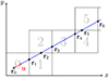 |
Fig. 1. Extension of the integration domain along the line of sight with the direction u, using repetition of the IllustrisTNG simulation boxes in the xy plane. |
In each simulation box, the line of sight intersects gas cells of variable comoving gas density  , mass m, free electron abundance χe, and comoving magnetic field
  . The comoving electron density in the cell is
  , where XH is the hydrogen mass fraction, and mp is the proton mass. The comoving cell size can be calculated assuming spherical symmetry
  . We calculated the distance d between the line of sight and the center of the gas cell to determine whether the line of sight intersects the cell: d < rcell (see Fig. 2).
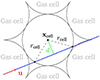 |
Fig. 2. Passage of the line of sight through an IllustrisTNG gas cell at the closest distance d from the center of the cell. The cell radius rcell may vary from one cell to the next. |
For each ith cell intersecting the line of sight, we extracted the components of the comoving magnetic field  and calculated its line-of-sight component
  . We also extracted the electron abundance χe and the gas density
  to calculate the expression under the RM integral in Eq. (4),
 (5)
(5)
We then defined Nz = 105 redshift grid points between z = 0 and z = 1.5, homogeneously spaced by Δz = 1.5 × 10⁻⁵, and interpolated the values of fi on this grid. We then calculated the RM along each line of sight as a sum:  .
.
Figure 3 shows the result of the calculation for one example line of sight. Large increments of the RM are typically found when the line of sight passes closer to a galaxy and possibly intersects one of the magnetized bubbles produced by the baryonic outflows. The probability of a crossing like this increases with redshift and all lines of sight eventually cross at least one magnetized bubble.
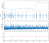 |
Fig. 3. Redshift variations of the RM. From top to bottom: parallel component of the magnetic field, electron density, and overdensity along one line of sight that intercepts an overdensity greater than 50 (horizontal red line) at z ≈ 1.1. |
Figure 4 shows a histogram of the RM values for a sample of 104 randomly generated lines of sight. The RM distribution does not correspond to a Gaussian function with the associated RM root mean square (rms). Furthermore, a number of outliers characterized by a large RM that correspond to the cases when the line of sight occasionally crosses a galaxy or galaxy cluster are present. The analysis of Carretti et al. (2023) has shown that the RM sample of LoTSS mostly does not contain lines of sight passing through large overdensities of the LSS. To account for this fact in the generation of predictions for the RM from numerical simulations, Carretti et al. (2023) have found that the closest approach of the lines of sight to the sources used in the LoTSS RM dataset corresponds to gas cells with overdensities  (
( is the critical density of the Universe). To account for the absence of lines of sight passing through larger overdensities, Carretti et al. (2023) removed cells with densities higher than this limit from the integration along the lines of sight through their simulation volumes. We adopted the same approach and removed gas cells with overdensities higher than the threshold δthr = 50 from the integral of Eq. (4).
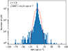 |
Fig. 4. Histogram of the RM values at z = 1.5 for a sample of 104 lines of sight with δ < 50. The distribution is centered around RM = 0 rad m−2, but does not follow a Gaussian distribution with a standard deviation |
5. Results
The IllustrisTNG simulation directly provides values of the intergalactic RM, while the RM values in observations are contaminated by the Galactic RM (GRM) foreground that needs to be subtracted to obtain the residual rotation measure (RRM) that includes the intergalactic RM and the RM intrinsic to the source and its host galaxy. The dashed lines in Fig. 5 show the redshift evolution of the rms of the RM calculated for a sample of 104 lines of sight through the IllustrisTNG with different gas cell overdensities. The RM quickly accumulates in the redshift range up to z ∼ 1 and stabilizes at higher redshifts. The main reason for the fast growth of the RM at low redshift is the presence of the magnetized bubbles driven by the baryonic feedback (Arámburo-García et al. 2021, 2022, 2023). These bubbles are most actively driven by star formation and AGN activity that peaks at somewhat higher redshifts. A stabilization of the RM at redshifts z > 1 indicates that the baryonic feedback-driven bubbles reach their highest volume-filling factor at redshift z ∼ 1. The seed cosmological magnetic field assumed in IllustrisTNG is at a level of 10−14 G, and its contribution to the RM is negligible compared to that of the outflow-driven magnetic field.
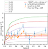 |
Fig. 5. Evolution of the rms of the RM with redshift in IllustrisTNG for six different overdensities in decreasing order from top to bottom (dashed lines). The measurements of the rms of the RRM derived from the LOFAR data (Carretti et al. 2023) based on the GRM model of Hutschenreuter et al. (2022) are shown in individual redshift bins (orange data points) with a power-law fit (orange line) and a constant |

Figure 5 also shows a comparison of the estimate of the RM from IllustrisTNG with the RRM extracted from the LOFAR data by Carretti et al. (2023). The overall RM measured by LOFAR has contributions from the GRM accumulated during the signal passage through the Milky Way galaxy, the RM accumulated during the signal passage through the intergalactic space, and RMIGM (of interest in this work) as well as the RM accumulated at the extragalactic radio source, RMlocal,
 (6)
(6)
An additional noise component arises from the limited precision of the measurements. The residual RM is obtained after subtraction of the GRM model from the total RM,
 (7)
(7)
By construction, the RRM includes the RM local to the radio source and the measurement noise, in addition to the RM accumulated in the IGM. Due to the presence of the noise and source components, the rms of the RRM is expected to be larger than the rms of the intergalactic RM component alone. Thus, the measurement of the rms of the RRM derived by Carretti et al. (2023)
 (8)
(8)
should be considered as an upper bound on the rms of the intergalactic RM,
 (9)
(9)
This upper bound is shown in Fig. 5 by a horizontal red line.
The LOFAR upper bound on the intergalactic RM contradicts the estimate of the RM extracted from the IllustrisTNG model already starting at redshift z ≃ 0.01. This conclusion is valid when the cut δ < 50 is imposed on the gas cells that are included in the RM integral, as explained in the previous section. At higher redshift, z ∼ 1, the discrepancy between the LoTSS upper limit and IllustrisTNG estimate reaches a factor of 3. Assuming redshift (z) and overdensity (δ) dependences, we can capture the shape of the curves from the IllustrisTNG simulation with a power-law fit f(z, δ) = aδzb, where a = 0.126 and b = 0.212 are constant parameters. Fitting the LOFAR data from Carretti et al. (2023), Fig. 5 shows that the model predictions can be made consistent with the data only when all the gas cells with an overdensity in excess of δthr ≃ 16.5 are removed from the RM integral of Eq. (4). This would efficiently remove parts of the lines of sight that pass through filaments of the LSS, which would not correspond to the realistic lines of sight from redshifts z ≳ 1 in the LoTSS sample, which are unlikely to completely avoid filaments.
6. Discussion
The contradiction between the estimate of the intergalactic RM from IllustrisTNG and LOFAR data shows that the model of magnetization of the intergalactic medium implemented in IllustrisTNG needs to be revised. The modeling shows that the RM along the lines of sight mostly accumulates in the magnetized bubbles around galaxies. This contrasts with the models considered by Carretti et al. (2023), in which the intergalactic RM was accumulated in filaments occupied by the compressed primordial magnetic field. This might be explained by the much stronger assumed initial field strength (∼10−10 G in Carretti et al. 2023 vs. 10−14 G in IllustrisTNG). Moreover, the IllustrisTNG baryonic feedback model prediction for the RM is dramatically different from the estimate of Carretti et al. (2023), where the astrophysical model of the magnetic field that is spread by galactic outflows failed to even produce an RM that reached the level that was observed by LOFAR. This perhaps demonstrates the wideness of the uncertainty range of the feedback parameters. Another possibility is that the phenomenological model of the outflows is correct, but that the numerical scheme used for the solution of the MHD equations overestimates the strength of the fields in the outflows (Hopkins & Raives 2016; Mocz et al. 2016).
O’Sullivan et al. (2023) and Carretti et al. (2023) reported that the GRM estimates of Hutschenreuter et al. (2022) are biased toward the RM measurements by LOFAR at the locations of sources from LoTSS, because the RM data sample used by Hutschenreuter et al. (2022) include LOFAR data of superior quality compared to the bulk of the RM data used for the GRM modeling. This led to an underestimate of the RRM. To overcome this difficulty, O’Sullivan et al. (2023) and Carretti et al. (2023) used the GRM model smoothed over one degree on the sky. To verify the estimate of the RRM of O’Sullivan et al. (2023) and Carretti et al. (2023), we compared the RRM estimate of O’Sullivan et al. (2023) and Carretti et al. (2023) with that derived from the same LOFAR data, but using the GRM model of Hutschenreuter & Enßlin (2020), which did not include LOFAR data. The result, shown by the blue data points in Fig. 5, shows that the two estimates are consistent with each other. The difference between the IllustrisTNG prediction and the RRM data is thus unlikely to be due to the underestimated RRM in the LOFAR data.
Even though the comparison of the IllustrisTNG model indicates that the model needs to be revised, it illustrates that the baryonic feedback field may readily saturate the bound on the intergalactic RM from LoTSS. This suggests that in contrast to the claim of Carretti et al. (2023), the presence of the 40 − 80 nG field found in the LSS filaments does not necessarily favor a model of the primordial stochastic magnetic field amplification in the filaments. Fields spread by galactic outflows with a somewhat reduced volume-filling factor compared to the IllustrisTNG model may well cause the fields found in the filaments.
One more important implication of our result concerns the possibility of measuring cosmological relic magnetic fields in the present-day Universe using the methods of γ-ray astronomy (Bondarenko et al. 2022). In the IllustrisTNG model, the magnetized outflows from galaxies are not strong enough to spread into the voids of the LSS with a large volume-filling factor (Arámburo-García et al. 2021, 2023). Our result shows that the IllustrisTNG model overestimates the strength of the outflows and suggests that the volume-filling factor of the outflows is smaller. This supports the idea that the large-scale magnetic fields in voids (Neronov & Vovk 2010; Acciari et al. 2023) have a cosmological origin.
Acknowledgments
We would like to thank F. Vazza, A. Boyarsky, K. Bondarenko and A. Sokolenko for their useful comments on the text. The IllustrisTNG simulations were undertaken with computing time awarded by the Gauss Center for Supercomputing (GCS) under GCS Large-Scale Projects GCS-ILLU and GCS-DWAR on the GCS share of the supercomputer Hazel Hen at the High Performance Computing Center Stuttgart (HLRS), as well as on the machines of the Max Planck Computing and Data Facility (MPCDF) in Garching, Germany.
References
- Acciari, V. A., Agudo, I., Aniello, T., et al. 2023, A&A, 670, A145 [NASA ADS] [CrossRef] [EDP Sciences] [Google Scholar]
- Arámburo-García, A., Bondarenko, K., Boyarsky, A., et al. 2021, MNRAS, 505, 5038 [NASA ADS] [CrossRef] [Google Scholar]
- Arámburo-García, A., Bondarenko, K., Boyarsky, A., et al. 2022, MNRAS, 515, 5673 [CrossRef] [Google Scholar]
- Arámburo-García, A., Bondarenko, K., Boyarsky, A., et al. 2023, MNRAS, 519, 4030 [CrossRef] [Google Scholar]
- Bertone, S., Vogt, C., & Enßlin, T. 2006, MNRAS, 370, 319 [NASA ADS] [Google Scholar]
- Bondarenko, K., Boyarsky, A., Korochkin, A., et al. 2022, A&A, 660, A80 [NASA ADS] [CrossRef] [EDP Sciences] [Google Scholar]
- Carretti, E., Vacca, V., O’Sullivan, S. P., et al. 2022, MNRAS, 512, 945 [NASA ADS] [CrossRef] [Google Scholar]
- Carretti, E., O’Sullivan, S. P., Vacca, V., et al. 2023, MNRAS, 518, 2273 [Google Scholar]
- Durrer, R., & Neronov, A. 2013, A&ARv, 21, 62 [NASA ADS] [CrossRef] [Google Scholar]
- Grasso, D., & Rubinstein, H. R. 2001, Phys. Rep., 348, 163 [NASA ADS] [CrossRef] [Google Scholar]
- Hopkins, P. F., & Raives, M. J. 2016, MNRAS, 455, 51 [NASA ADS] [CrossRef] [Google Scholar]
- Hutschenreuter, S., & Enßlin, T. A. 2020, A&A, 633, A150 [EDP Sciences] [Google Scholar]
- Hutschenreuter, S., Anderson, C. S., Betti, S., et al. 2022, A&A, 657, A43 [NASA ADS] [CrossRef] [EDP Sciences] [Google Scholar]
- Marinacci, F., Vogelsberger, M., Pakmor, R., et al. 2018, MNRAS, 480, 5113 [NASA ADS] [Google Scholar]
- Mocz, P., Pakmor, R., Springel, V., et al. 2016, MNRAS, 463, 477 [NASA ADS] [CrossRef] [Google Scholar]
- Naiman, J. P., Pillepich, A., Springel, V., et al. 2018, MNRAS, 477, 1206 [Google Scholar]
- Nelson, D., Pillepich, A., Springel, V., et al. 2018, MNRAS, 475, 624 [Google Scholar]
- Neronov, A., & Vovk, I. 2010, Science, 328, 73 [NASA ADS] [CrossRef] [Google Scholar]
- O’Sullivan, S. P., Shimwell, T. W., Hardcastle, M. J., et al. 2023, MNRAS, 519, 5723 [CrossRef] [Google Scholar]
- Pakmor, R., Bauer, A., & Springel, V. 2011, MNRAS, 418, 1392 [NASA ADS] [CrossRef] [Google Scholar]
- Pillepich, A., Nelson, D., Hernquist, L., et al. 2018, MNRAS, 475, 648 [Google Scholar]
- Planck Collaboration XIII. 2016, A&A, 594, A13 [NASA ADS] [CrossRef] [EDP Sciences] [Google Scholar]
- Sanati, M., Revaz, Y., Schober, J., Kunze, K. E., & Jablonka, P. 2020, A&A, 643, A54 [NASA ADS] [CrossRef] [EDP Sciences] [Google Scholar]
- Shimwell, T. W., Hardcastle, M. J., Tasse, C., et al. 2022, A&A, 659, A1 [NASA ADS] [CrossRef] [EDP Sciences] [Google Scholar]
- Springel, V. 2010, MNRAS, 401, 791 [Google Scholar]
- Springel, V., Pakmor, R., Pillepich, A., et al. 2018, MNRAS, 475, 676 [Google Scholar]
- Vachaspati, T. 2021, Rep. Prog. Phys., 84, 074901 [NASA ADS] [CrossRef] [Google Scholar]
- Vernstrom, T., Heald, G., Vazza, F., et al. 2021, MNRAS, 505, 4178 [NASA ADS] [CrossRef] [Google Scholar]
- Vernstrom, T., West, J., Vazza, F., et al. 2023, Sci. Adv., 9, eade7233 [NASA ADS] [CrossRef] [Google Scholar]
- Weinberger, R., Springel, V., Hernquist, L., et al. 2017, MNRAS, 465, 3291 [Google Scholar]
All Figures
|
Fig. 1. Extension of the integration domain along the line of sight with the direction u, using repetition of the IllustrisTNG simulation boxes in the xy plane. |
| In the text | |
|
Fig. 2. Passage of the line of sight through an IllustrisTNG gas cell at the closest distance d from the center of the cell. The cell radius rcell may vary from one cell to the next. |
| In the text | |
|
Fig. 3. Redshift variations of the RM. From top to bottom: parallel component of the magnetic field, electron density, and overdensity along one line of sight that intercepts an overdensity greater than 50 (horizontal red line) at z ≈ 1.1. |
| In the text | |
|
Fig. 4. Histogram of the RM values at z = 1.5 for a sample of 104 lines of sight with δ < 50. The distribution is centered around RM = 0 rad m−2, but does not follow a Gaussian distribution with a standard deviation |
| In the text | |
|
Fig. 5. Evolution of the rms of the RM with redshift in IllustrisTNG for six different overdensities in decreasing order from top to bottom (dashed lines). The measurements of the rms of the RRM derived from the LOFAR data (Carretti et al. 2023) based on the GRM model of Hutschenreuter et al. (2022) are shown in individual redshift bins (orange data points) with a power-law fit (orange line) and a constant |
| In the text | |
Current usage metrics show cumulative count of Article Views (full-text article views including HTML views, PDF and ePub downloads, according to the available data) and Abstracts Views on Vision4Press platform.
Data correspond to usage on the plateform after 2015. The current usage metrics is available 48-96 hours after online publication and is updated daily on week days.
Initial download of the metrics may take a while.