| Issue |
A&A
Volume 696, April 2025
|
|
|---|---|---|
| Article Number | A3 | |
| Number of page(s) | 16 | |
| Section | The Sun and the Heliosphere | |
| DOI | https://doi.org/10.1051/0004-6361/202453355 | |
| Published online | 28 March 2025 | |
High flow speeds and transition-region-like temperatures in the solar chromosphere during flux emergence
Evidence from imaging spectropolarimetry in He I 1083 nm and numerical simulations
1
Institute for Solar Physics, Dept. of Astronomy, Stockholm University, AlbaNova University Centre, SE-106 91 Stockholm, Sweden
2
Max-Planck-Institut für Sonnensystemforschung, Justus-von-Liebig-Weg 3, 37077 Göttingen, Germany
3
Institute of Theoretical Astrophysics, University of Oslo, PO Box 1029 Blindern, 0315 Oslo, Norway
4
Rosseland Centre for Solar Physics, University of Oslo, PO Box 1029 Blindern, 0315 Oslo, Norway
⋆ Corresponding author; jorrit.leenaarts@astro.su.se
Received:
9
December
2024
Accepted:
3
March
2025
Context. Flux emergence in the solar atmosphere is a complex process that causes a release of magnetic energy as heat and acceleration of solar plasma on a variety of spatial scales.
Aims. We aim to investigate temperatures and velocities in small-scale reconnection episodes during flux emergence.
Methods. We analyzed imaging spectropolarimetric data taken in the He I 1083 nm line with a spatial resolution of 0.26″, a time cadence of 2.8 s, and a spectral range corresponding to ±220 km s−1 around the line. This line is sensitive to temperatures higher than 15 kK, unlike diagnostics such as Mg II h&k, Ca II H&K, and Hα, which lose sensitivity already at 15 kK. The He I data is complemented by imaging spectropolarimetry in the Fe I 617.3 nm and Ca II 854.2 nm lines and imaging spectroscopy in Ca II K and Hα at a cadence between 12 s and 36 s. We employed inversions to determine the magnetic field and vertical velocity in the solar atmosphere. We computed He I 1083 nm profiles from a radiation-magneto-hydrodynamics simulation of the solar atmosphere to help in the interpretation of the observations.
Results. We find fast-evolving blob-like emission features in the He I 1083 nm triplet at locations where the magnetic field is rapidly changing direction, and these are likely sites of magnetic reconnection. We fit the line with a model consisting of an emitting layer located below a cold layer representing the fibril canopy. The modeling provides evidence that this model, while simple, catches the essential characteristics of the line formation. The morphology of the emission in the He I 1083 nm is localized and blob-like, unlike the emission in the Ca II K line, which is more filamentary.
Conclusions. The modeling shows that the He I 1083 nm emission features and their Doppler shifts can be caused by opposite-polarity reconnection and/or horizontal current sheets below the canopy layer in the chromosphere. Based on the high observed Doppler width and the blob-like appearance of the emission features, we conjecture that at least a fraction of them are produced by plasmoids. We conclude that transition-region-like temperatures in the deeper layers of the active region chromosphere are more common than previously thought.
Key words: magnetic reconnection / Sun: chromosphere / Sun: magnetic fields
© The Authors 2025
 Open Access article, published by EDP Sciences, under the terms of the Creative Commons Attribution License (https://creativecommons.org/licenses/by/4.0), which permits unrestricted use, distribution, and reproduction in any medium, provided the original work is properly cited.
This article is published in open access under the Subscribe to Open model. Subscribe to A&A to support open access publication.
1. Introduction
Flux emergence in the solar atmosphere is a complex process that causes a release of magnetic energy as heat and acceleration of solar plasma on a variety of spatial scales. In solar active regions, magnetic flux emerges from the convection zone into the photosphere on a variety of scales (Cheung & Isobe 2014). The associated magnetic flux ropes have an undulating character dipping into and out of the convection zone (Pariat et al. 2004). The emerging magnetic field reconnects with itself at progressively larger scales and interacts with previously emerged fields until longer loops are formed that can span from one polarity in the active region to the other (e.g., Ortiz et al. 2016). The flux emergence is associated with heating of the chromosphere as evidenced by the increased brightness and radiative losses in active regions compared to quiet Sun (e.g., Withbroe & Noyes 1977).
Flux emergence is associated with various brightening events and acceleration of plasma on a variety of scales (e.g., Nóbrega-Siverio et al. 2024). On sub-granular scales, self-reconnection in the photosphere gives rise to Hα Ellerman bombs (EBs, e.g., Georgoulis et al. 2002; Watanabe et al. 2011); at larger heights this process might appear as a UV-burst in observations of the Si IV 140 nm line (e.g. Peter et al. 2014; Vissers et al. 2015, 2019). On scales on the order of a few granules, reconnection and electric currents give rise to thread-like brightenings in Ca II H&K and Ca II infrared triplet lines as well as a more diffuse brightening surrounding the flux emergence sites (de la Cruz Rodríguez et al. 2015a; Leenaarts et al. 2018). On scales exceeding 10 arcseconds, chromospheric fibrils can become bright all along their length (Ortiz et al. 2016).
Currents sheets associated with magnetic reconnection are susceptible to the tearing instability and tend to fragment, forming magnetic islands or plasmoids in 2D geometry, and a complex structure of twisted magnetic flux ropes in 3D geometry (see Sect. 8 of Pontin & Priest 2022, and references therein). In simulations, these plasmoids have a typical size ranging from order one to a hundred kilometers, at the limit or below the diffraction limit of a meter-class telescope. They have a complex internal structure, with plasma at chromospheric and transition region temperatures lying close together and substantial velocity gradients. In 2D geometry, they are expelled from the reconnection site with speeds on the order of the Alfvén velocity. In observations, plasmoids appear as small bright blobs in the Ca II H&K and Hα lines (Rouppe van der Voort et al. 2017, 2023; Díaz Baso et al. 2021).
Ellerman bombs and UV bursts and their observational signature have been modeled using 3D radiation-magneto-hydrodynamics (MHD) simulations (Danilovic et al. 2017; Danilovic 2017; Hansteen et al. 2017, 2019). Current sheets did not fragment into plasmoids and small-scale twisted flux ropes in these simulations because of the limited resolution in such 3D simulations.
Resolution in 2D simulations is much less of a concern, and plasmoid formation in 2D under chromospheric and transition-region-like circumstances has been simulated by various authors (e.g., Ni et al. 2015; Rouppe van der Voort et al. 2017; Guo et al. 2020). Cheng et al. (2024) performed 2D simulations with adaptive mesh refinement of flux emergence with a resolution of ∼1 km. The simulation exhibited turbulent reconnection and plasmoid formation in the chromosphere away from photospheric flux cancellation sites. It is more reminiscent of reconnection when emerging short loops are pushed into preexisting longer loops.
The high-temperature gas present during reconnection cannot be seen with Mg II h&k, Ca II H&K, and Hα because their ionization stages have too low of a population at temperatures above 15 kK. Spectral lines in the UV offer this sensitivity but can only be observed from space. Slit spectroscopy of the Si IV 140 nm lines with the Interface Region Imaging Spectrograph (IRIS; De Pontieu et al. 2014) has been very successful at a resolution of 0.35″, but it requires scanning to obtain images, lowering the time resolution.
The atomic structure of He I makes the He I 1083 nm line sensitive to temperatures above 15 kK, and it is observable from the ground, making it a unique diagnostic for studying heating in the chromosphere. The reason for the sensitivity at high temperatures is that the triplet system of He I is only significantly populated through either recombination from He II if illuminated by UV radiation (Goldberg 1939), or bombardment by a non-thermal electron beam (Ding et al. 2005; Kerr et al. 2021), or through direct collisional excitation (Milkey et al. 1973). The latter mechanism requires temperatures in the line-forming region higher than 20 kK, the former two do not.
The line is normally in absorption, and the spatial variation of the line strength is mainly caused by the variation of the UV flux impinging on the chromosphere (Leenaarts et al. 2016). However, the line can show emission in EBs (Libbrecht et al. 2017) and flares (e.g., Zeng et al. 2014).
Libbrecht et al. (2021, hereafter L21) investigated the formation of the He I 1083 nm line in the simulations of a reconnection-driven bidirectional jet of Hansteen et al. (2019). They self-consistently included UV radiation produced by hot regions in the simulation, but did not include the effect of non-thermal electrons. They found He I 1083 nm line profiles in emission relative to the continuum intensity. Population in the triplet system was driven by UV radiation produced by a pocket of material at coronal temperatures in the chromosphere, while the emission itself was caused by a shell of material of chromospheric temperature around this hot pocket of sufficient optical thickness to cause the source function to thermalize.
Direct collisional excitation of the triplet system in 3D MHD simulations has to our knowledge not been reported, but there is no a priori reason why this would not occur given sufficient material at the right combination of temperatures and densities. However, as argued by Zeng et al. (2014), there is only a limited range of temperatures where this excitation can populate the triplet system without also collisionally ionizing most He I to He II. Non-equilibrium ionization could sustain He I at temperatures higher than where it would be ionized away in equilibrium circumstances, but only for a short time (ranging from ∼100 s at 23 kK, to 0.05 s at 93 kK). On the other hand, the optical thickness of the emitting layer does not need to be large to create emission relative to the continuum, because both the photon destruction probability ϵ and the Planck function are steeply increasing functions of temperature.
Collisional ionization by non-thermal particles would act the same as photo-ionization, but requires non-thermal particles inside small-scale reconnection events. To our knowledge, no observational evidence for this has been reported.
Here we use the first science-ready integral-field spectropolarimetry data in the He I 1083 nm line obtained with the Helium Spectropolarimeter (HeSP) instrument at the Swedish 1-m Solar Telescope to study small-scale reconnection events. We analyse the data using inversions and use radiation-MHD simulations of the solar atmosphere combined with non-LTE radiative transfer calculations of the He I 1083 nm to interpret the observations.
2. Observations and data reduction
We use observations from the Swedish 1-m Solar Telescope (Scharmer et al. 2003) taken on 2023-06-29 from 08:48:41UT to 09:01:43UT.
The CRISP imaging spectropolarimeter (Scharmer 2006; Scharmer et al. 2008; de Wijn et al. 2021) observed the Fe I 617.3 nm line, Hα, and the Ca II 854.2 nm with a cadence of 36 s. The Fe I 617.3 nm line was sampled with full-Stokes polarimetry at 11 wavelength positions equidistantly spaced from −17.5 pm to +17.5 pm around line center and a single point in the nearby continuum at +42 pm from line center. Hα was sampled at 19 equidistant positions from −90 pm to +90 pm around line center with spectroscopy only. The Ca II 854.2 nm was sampled equidistantly with 15 points from −67.5 pm to +67.5 pm around line center with full-Stokes polarimetry. The pixel scale was 0.044 arcsec.
The CHROMIS imaging spectrograph (Scharmer 2006, 2017) sampled the Ca II K line at 4 points placed at ±150 pm, ±117 pm, and at 25 points spaced equidistantly between −91 pm and +91 pm around line center. A point in the nearby continuum at λ = 400 nm was observed as well. The cadence of the CHROMIS observations was 11.8 s, and the pixel scale 0.038 arcsec. The CRISP and CHROMIS data were reduced with the SSTRED pipeline (de la Cruz Rodríguez et al. 2015b; Löfdahl et al. 2021). The polarimetric calibration of the CRISP data was performed by using a field-dependent demodulation matrix (as proposed by van Noort & Rouppe van der Voort 2008).
A recent addition to the instrumentation, the Helium Spectropolarimeter (HeSP) observed the He I 1083 nm line and the nearby Si I 1082.7 nm line with full-Stokes polarimetry. The HeSP is a microlensed hyperspectral imager (MiHI van Noort et al. 2022), specifically optimized for the helium line at 1083 nm, with a field-of-view (FOV) of 59 × 67 spatial pixels, each with an angular size of 0.13 arcsec, which approximately corresponds to critical sampling according to the Rayleigh criterion at this wavelength, yielding a FOV of 7.7″ × 8.7″. The spectral domain is sampled with 4 pm pixels from 1082.2 nm to 1083.8 nm corresponding to a Doppler speed of about ±220 km s−1 around the He I 1083 nm line. The raw HeSP data were reduced with a procedure closely following the one used for the MiHI prototype (van Noort et al. 2022; van Noort & Chanumolu 2022; van Noort & Doerr 2022).
The HeSP cameras operate at a framerate of 113.6 Hz. In sit-and-stare mode, as in the observations used here, the cadence of the reduced data can be decided after the observations. Here we reduced the data with a cadence of 2.8 s. The resulting HeSP data cubes have the same format as for Fabry-Pérot instruments like CRISP and CHROMIS: they contain intensity as function of time, spatial position, wavelength and Stokes parameter. The difference is that with HeSP all wavelengths are observed simultaneously, whereas Fabry-Pérot instruments observe different wavelengths consecutively.
Based on the root mean square (RMS) variations of the noise in the continuum on the red side of the lines, we estimate the noise floor to be about 1 × 10⁻² of the continuum intensity for a single (x, y, λ) pixel.
The target was the active region NOAA 13354. CRISP, CHROMIS, and HeSP have overlapping fields-of-view (FOVs) and observed cotemporally. The small HeSP FOV was approximately centered on (x, y) = (80″, 200″) in helioprojective Cartesian coordinates (corresponding to μ = 0.98), more or less in the middle of the FOV of the other two instruments (see Fig. 3).
The CRISP, CHROMIS, and HeSP data were coaligned to within one CHROMIS pixel, and resampled in space to the CHROMIS pixel scale of 0.0379″. The resampling of the HeSP data was done using nearest neighbor interpolation, for CRISP data linear interpolation was used. We chose to use nearest neighbor interpolation for HeSP because the large difference in spatial resolution between the He I 1083 nm and Ca II K would otherwise lead to artificially smooth HeSP images. The CRISP and CHROMIS data was resampled in time to the HeSP cadence of 2.8 s using nearest-neighbor interpolation, again to avoid artificial smoothness, but now in the time dimension. We chose not to rotate the data such that solar north points up to avoid unnecessary smoothing of the data. Therefore, the origin and orientation of the x and y axes in the figures are arbitrary.
Figure 2 shows an example frame of the HeSP data. The images appear sharp and at diffraction-limited resolution, and the spectra show strong variation on sub-arcsecond scales. The He I 1083 nm line is mostly in absorption, but also exhibits strong emission at certain locations in the FOV.
Because of the limited signal-to-noise ratio per pixel, Stokes Q and U are far above the noise in the Si I 1082.7 nm only, but the photospheric Ca I and Na I lines (see Fig. 1) also show a weak signal. The removal of the telluric water lines introduces weak spurious Q and U signal. In He I 1083 nm, Q and U are clearly above the noise only at a few locations, such as the Q vs λ plot and the xλ-cut in the upper right of the figure. In contrast, Stokes V is clearly visible in He I 1083 nm in many locations in the image and the spectra.
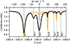 |
Fig. 1. Average spectrum and most important spectral lines in the HeSP observations. Black: spatially and temporally averaged HeSP observations. Orange: Atlas profile from Neckel & Labs (1984), arbitrarily scaled to match the continuum of the HeSP data. Solar spectral lines are indicated with dashed vertical lines and telluric water lines with dotted lines. |
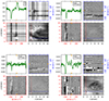 |
Fig. 2. Example HeSP snapshot, at 31 s after the start of the observations. The four groups of four panels display Stokes I (upper left), Q (upper right), U (lower left), and V (lower right). Each group consists of four subpanels, showing an example line profile (upper left), an xλ-slice (upper right), a λy-slice (lower left) and an xy-image (lower right). The locations of the xλ and λy-slices are indicated with blue and red dotted lines in the image, and their intersection is the location for which the line profile is shown. The wavelength of the Stokes Ixy-image in the lower-right is indicated with the orange tick marks in the Stokes I line profile in the upper-left. The Q, U, and V images are wavelength averages, with the average taken over the interval indicated by the orange ticks in the respective frames. The Stokes I intensity is given in arbitrary units. The wavelength axes are specified in units of Doppler velocity relative to λ = 1083.0 nm. An animated version of the figure is available online. |
3. Inversions
3.1. Inversions of the Fe I 617.3 nm and Ca II 854.2 nm lines
The Fe I 617.3 nm data was used in a spatially-regularized Milne-Eddington inversion following de la Cruz Rodríguez (2019) to estimate the photospheric magnetic field vector.
We obtained an estimate of the chromospheric magnetic field vector by applying a spatially-regularized weak-field approximation method to the Ca II 854.2 nm data following Morosin et al. (2020). We did not attempt to resolve the 180-degree ambiguity in the plane-of-the-sky (POS) in either of these inversions.
3.2. Inversion of the He I 1083 nm line
Selected pixels in the He I 1083 nm data were inverted using the HAZEL-2 code (Asensio Ramos et al. 2008), which can treat the full quantum formation of the He polarized signals including the Hanle, Zeeman and Paschen-Back effects. HAZEL-2 solves the radiative transfer in a constant-property slab model using a five-term atomic model for triplet state helium taking into account only radiative transitions. The emergent intensity is determined via an analytical solution to the polarized radiative transfer equation given by
![$$ \begin{aligned} \mathbf{I}=\mathrm{e}^{-\mathbf{K ^{*}}\Delta \tau }\,\mathbf{I}_{0}\,+\,\left[\mathbf{K ^{*}}\right]^{-1}\, \left( \mathbf 1 - \mathrm{e}^{-\mathbf{K ^{*}}\Delta \tau } \right)\,\beta \mathbf S . \end{aligned} $$](/articles/aa/full_html/2025/04/aa53355-24/aa53355-24-eq1.gif)
The quantity I0 is the Stokes vector incident on the boundary of the constant-property slab, furthest from the observer, and along the same line-of-sight. K* is the propagation matrix normalized by its first element (ηI), Δτ is the optical thickness of the slab, and S is the source function vector. The quantity β is an ad hoc scalar parameter that scales the source function to account for deviations from the collision-free case. We treat it as a free parameter. In the optically thin case β is ill-constrained and better kept fixed at unity, but for the pixels that we invert this is not the case.
The version of HAZEL-2 that we employ inverts the photospheric Si I 1082.7 nm line to provide an estimate of the incoming intensity I0 for the first slab above the photosphere. This photospheric inversion is done with the Stokes Inversion based on Response functions code (SIR; Ruiz Cobo & del Toro Iniesta 1992), that assumes LTE and hydrostatic equilibrium to solve the radiative transfer equation.
Here we focus the inversions on those pixels which show emission in the He I 1083 nm line. The observations show a dark layer of fibrils in the core of He I 1083 nm covering most of the FOV, and giving the impression that these fibrils are located higher in the atmosphere than most sites that produce the emission (see also Sect. 5.2 and Fig. 4).
Radiative transfer modeling of an Ellerman bomb/UV burst by L21 indicates that the contribution function of the He I 1083 nm is non-zero in only a few layers of only roughly 100 km extent in the vertical direction.
Taken together this led us to use HAZEL-2 with a stacked two-slab model, one located deeper down in the atmosphere, which we assume to be the emission site, and one slab higher in the atmosphere that represents the dense canopy of fibrils. The intensity from the photosphere is fed into the emission site slab, and the intensity from this slab is used as a boundary for the fibril slab. A similar approach was used in Libbrecht et al. (2017).
Owing to the noise level (of 10−2 in units of continuum intensity) and weak linear polarization signals in our FOV, we will not be able to infer the horizontal component of the magnetic field, so these parameters are kept at zero Gauss.
In order to characterize the incident radiation field, we need to specify the heights of our slabs above the photosphere. In our case, these cannot be inferred since we observe the region from above. We assumed a height of 2.2 Mm for the emission site slab as well as for the fibril canopy slab. While using the same height is unphysical, we cannot determine the heights of the slabs in our observations, so we stick with a single value for simplicity. The polarization signals are relatively insensitive to the exact values of the heights, and might lead to variations in the inferred field on the order of 10 G, so this is not important for our results (Díaz Baso et al. 2019a,b).
In total there are sixteen free parameters per pixel: we fit three nodes in temperature and one in line-of-sight velocity in the photospheric inversion. In each of the two slabs we fit the line-of-sight magnetic field BLOS, the optical thickness at the center of the red blended component of the He I 1083 nm multiplet Δτ, the line-of-sight velocity vLOS, the source function scaling factor β, the line width ΔvD and the damping parameter of the Voigt profile a.
We use the FAL-C model (Fontenla et al. 1993) as starting guess model for the photosphere. Some manual intervention was needed for the He slabs to converge to the best-fit solution. We achieve satisfactory fits using the strategy described below (see Sect. 5).
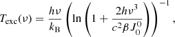
HAZEL-2 does not solve the full non-LTE problem. Instead, the source function is parametrized as a factor β times the first irreducible spherical tensor component of the radiation intensity J00, which is equal to the angle-averaged intensity (neglecting the minor contribution from J02):
The intensity I(ν, μ) used here is computed from the continuum irradiation from the solar photosphere. It takes into account the assumed height of the slabs, the center-to-limb variation and the wavelength dependence of the solar continuum radiation field I(ν, μ) as given in Allen’s astrophysical quantities (Cox 2000).
Because we assumed the height of our slabs to be constant, we can compute the excitation temperature (Rutten 2003) as function of β:
where h is the Planck constant and kB is the Boltzmann constant. For β = 1, we find Texc = 4.6 kK, for β = 10 we obtain Texc = 13 kK. We do not find solutions with β < 1, and the excitation temperature can therefore be interpreted as a lower bound of the gas temperature in the slab assuming the He I 1083 nm source function is described well by a two-level source function:

with ϵ being the photon destruction probability. We note that we cannot determine ϵ from our inversions. However, by definition 0 < ϵ < 1, which in turn implies J00 < Sν < Bν when β > 1, as is the case in our inversions.
4. Numerical modeling
To help interpret the observations, we employed a snapshot from a radiation-MHD simulation of the solar atmosphere, and solved the non-LTE radiative transfer problem for the He I 1083 nm line for this snapshot. The 3D model atmosphere was produced with the MURaM code (Vögler et al. 2005; Rempel 2017). The simulation is the flux emergence run 1 from Danilovic (2023). It tries to reproduce flux emergence in a mildly active region of the Sun. A bipolar flux system is advected through the bottom boundary into a fully developed plage simulation that includes subsurface layers, down to 8 Mm, photosphere, chromosphere, and corona up to 14 Mm. The emergence is limited within an ellipsoidal area with a major and minor axis (a, b) = (10, 2) Mm and field strength of 5000 G (Cheung et al. 2019). The emerging flux reaches the surface after approximately 5 hours of solar time. The grid spacing in the simulation domain is then reduced to half of the original value so that the final resolution is 39 and 21 km in the horizontal and vertical direction, respectively. The simulation domain is 40 × 40 × 22 Mm.
We used a snapshot from the simulation as input atmosphere for the 3D non-LTE radiative transfer computation performed with the Multi3d code (Leenaarts & Carlsson 2009). The input electron density was computed assuming LTE.
Multi3d solves the statistical equilibrium equations using the formalism of Rybicki & Hummer (1992), where the radiation field is evaluated in 3D using 24 angles in the A4 set of Carlson (1963). Because the photoionization-recombination mechanism is an essential mechanism that drives the population of the triplet system of He I, we included production of UV photons in the transition region and corona for wavelengths shortward of the He I ionization edge at 50.4 nm The coronal emissivity is computed as jν = Λν(T)nenH, where Λν(T) is computed using the CHIANTI package (Dere et al. 2009) assuming coronal equilibrium. This emissivity is added to the background emissivity in Multi3d. A detailed description of this method is given in Leenaarts et al. (2016).
We use the He model atom described in L21 It consists of 16 energy levels, of which 12 levels are in He I, 3 are in He II, and the final one is the He III continuum. The model includes the 1s 2s 3S1 and 1s 2p 3P0, 1, 2 levels that produce the three components of the He I 1083 nm line. A detailed description of the model atom including a term diagram is given in L21
In addition, we computed the emergent Hα intensity with Multi3d using full 3D non-LTE radiative transfer following Leenaarts et al. (2012) and the Ca II K intensity in non-LTE including the effects of PRD in the 1.5D approximation using the STiC code (de la Cruz Rodríguez et al. 2019; Uitenbroek 2001).
In addition to these new calculations, we also use a snapshot of a radiation-MHD simulation computed with the Bifrost code by Hansteen et al. (2019) to interpret our observations. The radiative transfer problem for He in this snapshot was solved by L21. This snapshot contains an Ellerman-bomb/UV-burst small-scale reconnection event which shows emission in the He I 1083 nm line.
5. Results
5.1. Overview of the observed region
Figure 3 shows an overview of the observed active region (AR) NOAA 13354 based on the CRISP data. The AR harbours two groups of sunspots of opposite polarity. One group is inside the CRISP FOV, the second group is outside the FOV at the lower right of the figure. Inspection of SDO/HMI data of the AR shows that most flux had emerged by the time of the observations, but the sunspot groups continued to separate for a few days after this date, and flux emergence was still ongoing during the observations. This is evidenced by the elongated structures visible in the continuum intensity between the sunspot groups and the corresponding elongated photospheric magnetic field structures of both polarities visible in BLOS. The HeSP FOV is located in this area with flux emergence. The Hα image shows thick fibrils covering most of the FOV. The photospheric LOS magnetic field structure within the FOV is markedly different from, and predominantly of the opposite polarity as the field in the nearby penumbra.
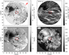 |
Fig. 3. Overview of the observed region at 2023-06-29T08:49, the start of the observation. The upper row shows the continuum close to the Fe I 617.3 nm line and the Hα line core. The bottom row shows the line-of sight and plane-of-the-sky components of the photospheric magnetic field, as determined from the spatially-coupled Milne-Eddington inversion of the Fe I 617.3 nm. The red box shows the HeSP FOV and the arrow in the upper left panel points toward solar north. |
5.2. Zoom in on the HeSP field of view
Figure 4 shows the HeSP FOV. It contains a number of small pores with different polarity (panels a and m).
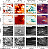 |
Fig. 4. Overview of the HeSP FOV at 246 s after the start of the observations. First row (a–d): magnetic field in the photosphere as determined from a Milne-Eddington inversion of the Fe I 617.3 nm recorded by CRISP. Second row: magnetic field in the chromosphere as determined from the weak-field approximation in the Ca II 854.2 nm (also CRISP data). Bottom two rows: intensity images at various wavelengths. The Hα red wing image is at Δλ = +45 km s−1 from the nominal line core, the Ca II K red wing image at Δλ = +36 km s−1. Panel j shows the intensity normalized to the local continuum intensity I(x, y, λ)/Icont(x, y), the other panels show the unscaled intensity I(x, y, λ). A movie of this figure showing the entire time series is available online. |
The photospheric magnetic field is rather vertical in the pores, but the FOV contains patches with kG-strength horizontal field as well (such as (x, y) = (9″, 7″)), indicative of flux emergence. The azimuth of the magnetic field is predominantly NW to SE, except around the pores at y = 4″, where the azimuth structure appears more complex.
The second row of the figure shows the chromospheric magnetic field as determined from the Ca II 854.2 nm line. The vertical chromospheric field (panel e) is much smoother than in the photosphere and has a lower unsigned field strength. Comparison with panels e and o shows that the positive LOS magnetic field is associated with the dark fibrils covering much of the FOV. Where the fibrils are not present the LOS magnetic field is negative. There are two elongated patches of strong vertical field at y = 4″ and y = 6″. The horizontal field and the inclination (panels f and g) show that in these patches the field is much more vertical. The azimuth panel shows that the horizontal direction of the field largely follows the orientation of the fibrils, except in a small area around (x, y) = (7″, 4.5″), where the azimuth is roughly 90 degrees different.
The picture emerging from this analysis is that there is ongoing small-scale flux emergence in the photosphere with opposite polarity fields existing close together and a complex structure of the horizontal direction of the field. The overlying upper chromosphere appears to consist mostly of ordered fibrils as seen in Hα and Ca II K which are much longer than the extent of the HeSP FOV (see Fig. 3). The atmosphere between the photosphere and the fibril canopy is therefore expected to show a complex evolving magnetic field exhibiting small-scale reconnection and current sheets with concomitant heating, flows and jets (e.g., Ortiz et al. 2020; Díaz Baso et al. 2021).
This view is corroborated in panels l and p, which show images at wavelengths in the red wing of the lines, chosen such that they show a scene in between the photosphere and the fibril canopy. The Ca II K panel in particular is filled with elongated intermediate-brightness threads, which are sites with elevated temperature (e.g. Leenaarts et al. 2018). It also shows blobs and shorter threads with high brightness. The Hα panel shows fewer and less pronounced intermediate-brightness threads, but does show some high-brightness blobs and threads that partially coincide with the ones visible in Ca II K. These phenomena are not visible in the core of the Fe I 617.3 nm (panel n), indicating that the heating is occurring at least 100–200 km higher than the local formation height of the continuum (e.g. Smitha et al. 2023).
Finally, we turn to the appearance of the He I 1083 nm line. The figure does not show the 1083 nm continuum, but inspection shows it appears largely similar to the 400 nm continuum in panel m, but with lower contrast and lower spatial resolution owing to the longer wavelength. The line core (panel i) shows fibrils with the same overall orientation as in the Hα and Ca II K line cores. They appear thinner and not as dark, but are nevertheless completely optically thick, and no photospheric structure is visible. This is expected in active regions where the hot and dense corona produces copious amounts of UV photons to drive the photoionization-recombination mechanism that populates the triplet system of He I.
Panel j shows the intensity at λ = 1083.11 nm, in the red wing of He I 1083 nm, divided by the local continuum intensity, that is, I(x, y, λ)/Icont(x, y). Dividing by the continuum makes the background appear flat, emission above the local continuum level appears bright and absorption features appear dark. The most prominent features are the emission structures at (x, y) = (6″, 4″). Inspection of the movie of Fig. 4 shows that the emission appears as roundish blobs with a diameter smaller than  to elongated blobs of up to 2″ length and a width below
  . Often, but not always there is emission in the red wings of Ca II K, and Hα at locations of He I 1083 nm emission. The reverse is not true, many bright structures visible in Ca II K, such as the threads at (x, y) = (2″, 3″) and (x, y) = (9″, 1.5″) do not have a counterpart in He I 1083 nm. The He I 1083 nm wing image also does not show the elongated intermediate brightness threads that are present in the red wing of Ca II K.
The He I 1083 nm emission is not confined to the red wing of the line, but sometimes appears as wide emission humps as illustrated in Fig. 5. The most extreme profiles exhibit emission out to large Doppler shifts from the line core, ranging from 180 km s−1 blueshift to 140 km s−1 redshift.
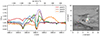 |
Fig. 5. Example He I 1083 nm line profiles that show emission. Left: line profiles. Right: local continuum normalized intensity in the red wing of He I 1083 nm, with the locations of the profiles left indicated with squares of the same color as the profile. The line profiles are taken from the entire time series, not just from the timestep shown in the right-hand panel. The labeled line profiles are discussed in Sects. 5.4–5.6. |
5.3. Analysis of emission sites
In the following sections we present a deeper analysis of three representative pixels that show emission. These pixels are designated as follows: pixel A (red in Fig. 5), pixel B (brown), and pixel C (orange). Figures 6–8 show the locations of these pixels, their time evolution and a comparison with the Ca II K line. Figure 9 shows the fits obtained with the stacked-slab inversions as described in Sects. 3.2, and the inferred parameters are given in Table 1. We note that the optical depth and source function in the emission slab suffer from significant degeneracy. The emission peaks tend to be well-fitted both by a modestly high source function and an optically thick slab, as well as a very high source function with a slab thickness below unity. We show examples of these two types of fits in Appendix A.
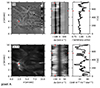 |
Fig. 6. Emission in pixel A. Upper left: image of the scaled intensity Iλ(x, y, t)/Icont(x, y, t) in He I 1083 nm. Upper-middle: λt-slice of the scaled intensity at the location of the red square in the image. The red tick marks indicate the wavelength and time of the image. Upper right: light curve at the spatial location indicated by the square and the wavelength indicated by the tick marks. The bottom row shows the same for Ca II K, except that the image in the lower-left panel shows Iλ, i.e., it is not scaled to the local continuum intensity. |
5.4. Pixel A
The He I 1083 nm line profile of Pixel A shows a very wide emission component that is located on top of the Si I 1082.7 nm line, raising the question of whether the emission is really caused by He I 1083 nm. Because the Si I 1082.7 nm line core is in absorption, the emission, were it caused by Si I, would have to be caused by a high source function deeper down than the Si I 1082.7 nm line core formation height of ≈500 km (Bard & Carlsson 2008). However, comparison with the movie of Fig. 4 shows that the emission is not visible in the Fe I 617.3 nm line and we conclude that the emission is indeed caused by He I 1083 nm.
Panel a of Fig. 4 and the corresponding movie show that the emission is located at a site of persistent photospheric magnetic flux cancellation. This cancellation causes persistent emission in Ca II K (panel l) and Hα (panel p) with an elongated shape. The line-core images (panels i and k) show a faint hint of the emission peeping through the fibril canopy, but is invisible in the Hα core (panel o). The persistence of the Ca II K emission is also clearly seen in the lower panels of Fig. 6. Taken together, we obtain a picture of reconnection brightening in the chromosphere, but clearly below the fibril canopy, reminiscent of Ellerman bombs.
In contrast, the He I 1083 nm emission is much more roundish and blob-like, and more intermittent in time as seen in the upper panels of Fig. 6. As can be seen by comparing the λt-plots in Fig. 7, the Ca II K brightness at times of the He I 1083 nm emission does not stand out.
The line profile is well-fitted by the Hazel inversion (Fig. 9). The upper slab that represents the fibril canopy is marginally optically thick (Δτ = 2, see Table 1), essentially at rest and with a LOS magnetic field strength that is below our noise limit. The layer that is responsible for the blueshifted emission has an upflow speed of 79 km s−1. The Doppler width has an unrealistically high value of 39 km s−1 corresponding to a temperature of ∼400 kK. This is too high for the existence of significant amounts of He I, even when accounting for non-equilibrium ionization (Zeng et al. 2014). The Doppler width should thus be interpreted as the presence of large velocity gradients along the line-of-sight and/or within a HeSP resolution element that cannot be fitted with a constant-property slab (see also Lagg et al. 2007). Likewise, the fitted value of the Voigt damping parameter a = 1.0 is unphysically large and must be interpreted as the inversion trying to fit unresolved velocity gradients, because even at photospheric densities the damping parameter is of order ≈0.01.
Retrieved parameters and associated uncertainties using the stacked HAZEL-2 slab model to the observed spectra.
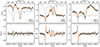 |
Fig. 9. Inversion results for the three selected pixels with emission in the He I 1083 nm line. The columns show the results for pixels A (left), B (middle), and C (right). The top row shows Stokes I; the bottom row Stokes V. Black-filled circles represent the observations, the orange solid lines are the best-fit profiles. The thin gray curve represents an average of a relatively quiet part of the FOV. |
5.5. Pixel B
Pixel B is part of a slightly larger brightening event with about one arcsec diameter located just outside of the fibril canopy, at (x, y) = (2″, 2″) in Figs. 4 and 7. It is located close to, but not on top of, the photospheric polarity inversion line, and is therefore probably not an Ellerman-bomb-like reconnection event. The emission in He I 1083 nm is as concentrated in time as in Ca II K. It is very bright for only 10 s after which the emission rapidly weakens and fades away completely after 30 s.
The Hazel inversion (Fig. 9) properly fits the Stokes I and V profiles. Because the emission is outside the fibril canopy, the properties of both the upper and the lower slab are likely set in the emission region. This is evidenced by the similar values of vLOS and ΔvD. The source function in the upper slab (β = 1) is lower than in the lower slab (β = 8) in order to fit the central reversal of the line. We speculate that the observed central reversal is just a consequence of scattering line formation where the source function drops below the Planck function at heights where the line core forms (similar to the formation mechanism of the central reversal in the Ca II H&K and Mg II h&k lines).
Interestingly, the Stokes V signal in this pixel is strong enough to fit a reasonable value of the LOS magnetic field, −509 G in the upper slab, and −665 G in the lower slab. Given the simplicity of the slab model, we do not believe that the inferred difference in field strengths is necessarily real, but it is clear that the emission forms in a layer with a magnetic field of about 0.5–0.6 kG. This is consistent with the value derived from applying the weak-field approximation to the Ca II 854.2 nm at the same location.
5.6. Pixel C
The brightening in Pixel C occurred at (x, y) = (6″, 4″) at t = 245 s above the pore in the middle of the FOV of HeSP, several arcseconds away from a photospheric polarity inversion line. It is part of a cluster of blobby or slightly elongated brightenings of sub-arcsecond size that appear to move to the left as time passes, as can be seen in panel j in the movie of Fig. 4. A second He I 1083 nm emission event occurs in the same area around t = 403 s. Inspection of the data (not shown here) reveals that most of the emission in this area shows either no clear Doppler shift, or shows redshift.
Comparison between the He I 1083 nm and Ca II K images in Fig. 8 shows that Ca II K is bright at the same locations as He I 1083 nm, but it also shows bright fibrils that emanate from the location of the He I 1083 nm emission. The Ca II K is more persistent in time as well, with persistently elevated brightness between t = 0 and t = 400 s.
The emission is neither visible in the line core of the photospheric Fe I 617.3 nm (Fig. 4n) nor the cores of the chromospheric He I 1083 nm and Ca II K lines, and the emission is thus most likely located in the mid-chromosphere, just as for Pixel A.
The inversion code fits the line profile well, and predicts an upper slab that is at rest, with a modest Doppler width. The lower slab, representing the emission site, exhibits a downflow of 67 km s−1. Just as for Pixel A, the fitted microturbulence is unrealistically high at 32 km s−1, indicating strong unresolved velocity gradients along the line of sight and/or within a HeSP resolution element. The inferred value of the LOS magnetic field in the lower slab is not reliable: the lower right panel of Fig. 9 shows that Stokes V in the emission hump is dominated by noise.
Because Pixel C is located away from a photospheric polarity inversion line, we deem Ellerman-Bomb-like reconnection an unlikely cause of this brightening. The azimuth of the magnetic field in the chromosphere shows an elongated patch of NE-SW orientation (blueish in Fig. 4h) that makes a roughly 90° angle with the predominant NW-SE orientation (red-brown in Fig. 4h). The He I 1083 nm brightening is located at the left end of this patch at x = 6 Mm. The inclination of the chromospheric field (Fig. 4g) shows two patches of a close-to-vertical field on both sides of the patch with NE-SW azimuth. The movie of Fig. 4 shows that the blue patch in azimuth starts to appear around t = 200 s, and has disappeared by t = 250 s.
The chromospheric magnetic field was inferred with the weak field approximation, and lacks information on the geometrical height of the inferred magnetic field. This means we cannot determine the detailed magnetic field configuration around Pixel C. Nevertheless, the large gradients in azimuth and inclination around Pixel C mean that the field must exhibit shear, which in turn implies the presence of electric currents, and possibly also magnetic reconnection.
6. Interpretation based on numerical modeling
The formation of the He I 1083 nm line in an Ellerman Bomb was studied by L21 based on a radiation-MHD simulation of flux emerging into the atmosphere by Hansteen et al. (2019). In this simulation, reconnection occurs in a long vertical current sheet in the chromosphere as a consequence of the squeezing together of opposite polarity flux in the photosphere. As a result, a sheet of material at coronal temperatures is formed, as well as a bidirectional jet. Figure 5 in L21 shows that the He I 1083 nm line profiles at this current sheet exhibit broad emission peaks with intensity up to twice the continuum intensity, and with Doppler shifts ranging from −100 km s−1 to +80 km s−1. Such profiles are reminiscent of the observed profiles presented in this work.
L21 present an analysis of the formation of one of their synthetic line profiles that exhibits both a redshifted and a blueshifted emission component in their Fig. 7, which shows a four-panel formation diagram following the format of Carlsson & Stein (1997).
The red-shifted component forms in the downward part of the bidirectional jet in an emitting layer of about 100 km thickness. This layer is located in a strong velocity gradient which causes a large non-thermal width, similar to what we find in our Hazel inversions. The blue-shifted emission component forms at a larger height, in the upflowing part of the bidirectional jet. It is likewise formed in a thin layer with a gradient in the vertical velocity. Finally, the line profile shows a central depression formed at even larger heights, and is caused by the overlying fibril canopy (see Fig. 4 in L21).
Our Pixel A is located above a patch of persistent photospheric flux cancellation and shows EB-like behavior, similar to the situation described in L21. The line profile in Pixel A can be well-fitted with only one emission component, which is blueshifted. We therefore interpret this emission as formed in the upwardly-directed reconnection outflow. Whether the reconnection gives rise to a bidirectional flow as in L21 requires full non-LTE inversions as in Vissers et al. (2019), which is beyond the scope of the present paper.
Pixel B is not located above a photospheric polarity inversion line. The magnetic field appears to be quite vertical in both the photosphere and chromosphere, even though there is a visible substructure in the inclination at the site of the brightening (see the movie of Fig. 4 around 36 s). The azimuth of the field in the chromosphere shows a large gradient of up to 90 degrees across the brightening (panel h in the movie). We could not infer a likely field configuration from the retrieved magnetic field information so we must refrain from interpreting this event based on the numerical modeling.
Pixel C is part of a complex of brightenings located in a region away from the bipolar magnetic field in the photosphere. The magnetic configuration in the chromosphere exhibits strong changes in the azimuth of the field. The snapshot analyzed by L21 did not contain such an event. Instead, we searched for and found one event in the MURaM simulation described in Sect. 4 that shows a brightening event in the He I 1083 nm associated with a rapid change of field azimuth with height.
The top row of Fig. 10 shows the entire simulation domain. There are two large elongated patches of strong photospheric field, and in between them, there is ongoing flux emergence (inside and above the red box). The He I 1083 nm line core shows a complex fibrillar structure that in general connects the patches of opposite polarity. The appearance of the fibrils in the line core is reminiscent of our observations (see Fig. 4i).
In the bottom row of Fig. 10 we show the region with the He I 1083 nm brightening. Panel c shows the local-continuum-divided He I 1083 nm intensity at a Doppler shift of Δv = −18 km s−1, and exhibits an elongated patch with intensity higher than the local continuum. The photospheric magnetic field in panel a shows the brightening is associated with field lines emanating from a unipolar photospheric magnetic field concentration, without significant opposite polarity flux nearby.
The brightening in the He I 1083 nm wing is not visible in the line core image in panel b. The blue wing of Hα (panel d) shows the same brightening, but the Ca II K (panel e) wing does not. Owing to the large difference in cadence between the Ca II K, Hα, and He I 1083 nm data we cannot be sure of the observational configuration, but Fig. 4 indicates the Pixel C event is visible in all three lines, in contrast to our simulation.
Figure 11 displays the line formation for the brightening through a four-panel formation diagram (Carlsson & Stein 1997) of the pixel indicated in the lower row of Fig. 10. The emission peaks are formed in a single thin layer at z = 1.5 Mm, where the line source function shows a sharp local maximum. This height is the τ = 1 height at the frequencies of the emission peaks in the line profile. The source function maximum is located right next to a thin layer with a maximum temperature of T = 29 kK. Determining whether the source function maximum is caused by the photoionization-recombination mechanism or direct collisional ionization and excitation would require the same extensive analysis as in L21, and because the effect on the line profile is the same, we refrain from doing that here. The emission layer shows a downflow with a speed of 12 km s−1. The absorption throughs are formed in a range of heights between z = 1.6 Mm and z = 2.4 Mm, where the material has a vertical velocity in the range from −5 km s−1 to +4 km s−1.
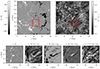 |
Fig. 10. Simulation data. Top row: Vertical component of the magnetic field at z = 0 km and emergent intensity at the nominal line core of the strong component of the He I 1083 nm line. Bottom row: zoom in of the region inside the red square in the top row. Panel a: Vertical component of the photospheric magnetic field at z = 0 km; panel b: emergent intensity at the nominal line core of the strong component of the He I 1083 nm.; panel c: local continuum scaled intensity of the He I 1083 nm at a Doppler shift of −18 km s−1; panel d: Hα intensity at a Doppler shift of −33 km s−1; panel e: Ca II K intensity at a Doppler shift of −8 km s−1. The pixel marked with the filled red square is analyzed in Fig. 11. |
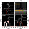 |
Fig. 11. Four-panel formation diagram of the pixel marked in red in the bottom row of Fig. 10. Top left: Opacity χν divided by optical depth τν. The red curve is the height optical depth is unity, the white vertical line marks Δν = 0 and the white curve is the vertical velocity as a function of height. Top right: total source function. The green curve shows the line source function, the orange curve the temperature. Bottom left: τνexp−τν, which peaks at τν = 1. Bottom right: the contribution function χνSνexp−τν. The white curve shows the emergent line profile in temperature units, with a scale on the right. |
This analysis shows that also for this type of event, our simple inversion model of a hot emitting layer below an absorbing cooler fibril layer appears valid. While the absorbing layer has a vertical extent of 0.8 Mm and shows a range of velocities, the source function in this layer is rather constant, and the inversion would likely be able to fit the profile with a single source function and some microturbulence. The downflow in the emitting layer, combined with the roughly zero velocity of the absorbing layer causes the leftmost emission peak to be lower than the other two (as seen of the relatively low value of χν/τν in the leftmost peak in the upper left panel of the figure).
In Fig. 12, we analyse the magnetic field configuration of the event. The material causing the emission peaks is located at the top of the red pillars in the middle of the image, which represent the z(τ = 1) at Δv = −18 km s−1 for the He I 1083 nm line. The magnetic field lines that thread this region are strongly sheared, and a current sheet (not shown in the figure) is located next to the emission region. This current sheet causes the high temperature at z = 1.4 Mm in Fig. 11. The sheet is so thin that even though some of the field lines intersect with the sheet, this high temperature is not visible in the figure.
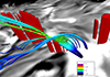 |
Fig. 12. 3D visualization of the magnetic field configuration of the He I 1083 nm emission event in our MURaM simulation. The greyscale background shows the vertical magnetic field in the photosphere (white: positive; black: negative), just above the continuum formation height. The red surface displays the height of optical depth unity z(τ = 1) for the vertically emergent intensity at Δv = −18 km s−1 for the He I 1083 nm line, corresponding to the blue wing images in Fig. 10. This height tends to lie below the height for which we display the magnetic field, and is above it only in some locations, appearing as steeply-sided columns. The magnetic field lines thread the emitting region of the He I 1083 nm brightening, and their color indicates the local temperature. Figure made with VAPOR (Li et al. 2019). |
The field lines originate from a unipolar region to the right of the current sheet. Even though there is opposite polarity flux right below the current sheet, this flux is unrelated to the sheet.
Based on the analysis of this event in our simulation we conclude that the observed behavior of pixel C is consistent with current sheets in the chromosphere caused by sheared magnetic field lines emanating from unipolar regions in the photosphere (see also Hansteen et al. 2015; Skan et al. 2023). The Joule heating inside the sheet can be sufficiently large to raise the temperature to at least 20 kK, sufficient for either the photoionization/recombination mechanism or direct collisional excitation to create He I 1083 nm opacity and a line source function larger than the source function in the photosphere.
7. Discussion and conclusions
In summary, we find small fast-evolving brightenings in the He I 1083 nm line in the observations. They are often cospatial with Hα and Ca II K brightenings, but the latter are much more persistent in time and extended in space. As He I 1083 nm only shows emission in or next to sites with temperatures above 20 kK, these emission sites must indicate small hot spots in the lower solar atmosphere, below the fibril canopy.
A two-layer inversion model can fit the observed He I 1083 nm profiles, and we find large upflows and downflows of order ±75 km s−1. These speeds are inconsistent with acoustic phenomena (the sound speed is of order 10 km s−1) as well as observed velocity amplitudes in transverse or torsional waves in spicules (De Pontieu et al. 2012) and fibrils (e.g. Morton et al. 2012; Kianfar et al. 2022).
These flow speeds are instead consistent with the Alfvén speed vA. Taking B = 665 G as found for the lower slab in pixel B, and a mass density ρ = 7 × 10⁻⁶ kg m−3, corresponding to z = 500 km in the FALC model atmosphere (Fontenla et al. 1993), we find vA = 22 km s−1. For ρ = 10−7 kg m−3, corresponding to z = 1000 km in FALC, vA = 188 km s−1.
Reconnection outflow speeds tend to be on the order of the Alfvén speed (e.g., Parker 1957; Priest 2014), and we interpret the speeds that we recover for pixels A and C as caused by such outflows. To our knowledge, this is the first time such line-of-sight flow speeds are measured in reconnection events at sub-arcsecond scales. Earlier inversions of Ellerman bombs and UV bursts based on Ca II K, Mg II h&k yielded velocities up to ±30 km s−1(Vissers et al. 2019). Inversions of Ellerman Bombs in the He I D3 and He I 1083 nm lines by Rouppe van der Voort et al. (2017) found velocities from 22 km s−1 downflows up to 40 km s−1 upflows. Díaz Baso et al. (2021) found plasmoids visible in the Ca II K line at a blueshift of 100 km s−1, but did not determine the flow speed with inversions.
Speeds of order 100 km s−1 derived from the He I 1083 nm line have been measured before (e.g. Sasso et al. 2011; Díaz Baso et al. 2019a; Sowmya et al. 2022), but with absorption components and for filaments and along chromospheric fibrils at larger spatial scales than reported here.
UV bursts seen in the Si IV 139.4 nm and 140.3 nm lines (Peter et al. 2014), are a signature of low-atmospheric reconnection. At least a fraction of them is caused by the same mechanism that produces Ellerman Bombs: the squeezing together of opposite polarity fields in the photosphere and chromosphere (Hansteen et al. 2019), and flow speeds up to ±100 km s−1 have been reported for them (Peter et al. 2014; Tian et al. 2018). UV bursts tend to have an observed size of order 1″–3″, substantially larger than our pixels A and C, but comparable to pixel B.
Magnetic reconnection in three dimensions is extremely complex and can occur in a variety of magnetic field configurations (Pontin & Priest 2022). We showed using 3D radiation-MHD simulations that some of the observed He I 1083 nm profiles are consistent with opposite polarity reconnection of vertically oriented field (pixel A, see L21) and current sheets in sheared largely horizontal field in the chromosphere (pixel C, simulation presented in this paper). The limited spatial resolution and concomitant large numerical resistivity and viscosity in these simulations mean that the reconnection current sheets lack significant substructure. The resulting He I 1083 nm profiles (Fig. 11 and L21) therefore do not exhibit the wide emission humps (requiring large non-thermal broadening to fit) seen in our observations (Fig. 5).
Long thin current sheets are however unstable and fragment into plasmoids (magnetic islands in 2D and twisted flux ropes in 3D, see Sect. 8 of Pontin & Priest 2022). This process has only been studied in 3D under idealized or coronal circumstances (e.g., Huang & Bhattacharjee 2016; Sen et al. 2023). In 2D it has been studied under chromospheric conditions in self-consistent 2D radiative-MHD simulations by Rouppe van der Voort et al. (2017). The exact spatial resolution of this simulation is not reported, but while the resolution was high enough to lead to fragmentation of the current sheet, the resulting plasmoids do not show internal substructure.
In the 2D simulations of Ni et al. (2021) and Cheng et al. (2024) adaptive mesh refinement was used to simulate plasmoids in the chromosphere with a spatial resolution less than one kilometer. They find plasmoids with a diameter of about 100 km, typically consisting of a hot (∼100 kK) and tenuous partial ring surrounding a dense core with a temperature less than 10 kK. The hot ring should produce copious amount of UV radiation that populates the He I triplet system through photoionization/recombination in the core as well as the surrounding undisturbed chromosphere (Leenaarts et al. 2016). They could thus well explain the small roundish emission features close to the diffraction limit that we find in our data.
In addition, the simulated plasmoids harbour substantial internal velocity structure, with flow speeds reaching up to about 20 km s−1. Because our observations have a spatial resolution of 200 km, we would not resolve the internal velocity gradients in the plane-of-the-sky direction. The vertical extent of the contribution function makes it impossible to resolve such a structure along the line-of-sight. These two effects combined offer a natural explanation for the wide emission humps and non-thermal velocities of order 40 km s−1 that we find in our inversions.
This study is an initial exploration of the first HeSP dataset. The reconnection brightenings are small, evolve fast and show structure at large Dopplershift from the nominal line center. Based on the temperature needed to produce them, we conclude that transition-region-like temperatures in the deeper layers of the active region chromosphere are more common than previously thought.
It highlights the power of high-cadence integral-field spectropolarimetry combined with image reconstruction to reach diffraction-limited spatial resolution. Neither slit spectrographs nor wavelength-scanning imaging instruments are able to fully characterize these events. The He I 1083 nm is a unique diagnostic to study small-scale reconnection and heating in the chromosphere through its sensitivity to temperature above 20 kK, where H I, Ca II, and Mg II are already ionized away.
The study also shows the importance of multiple diagnostics to constrain the physical interpretation. Work is underway to further analyse the He I 1083 nm brightenings through a more in-depth investigation of their motion, more extensive inversions with Hazel and full non-LTE inversions of the Ca II K, Fe I 617.3 nm, and Ca II 854.2 nm lines to better constrain the magnetic field configuration in these events. It would also be of interest to compute the He I 1083 nm profiles emanating from models of chromospheric plasmoids.
Data availability
Movies associated to Figs. 2 and 4 are available at https://www.aanda.org
Acknowledgments
The Swedish 1-m Solar Telescope is operated on the island of La Palma by the Institute for Solar Physics of Stockholm University in the Spanish Observatorio del Roque de los Muchachos of the Instituto de Astrofísica de Canarias. The Institute for Solar Physics is supported by a grant for research infrastructures of national importance from the Swedish Research Council (registration number 2021-00169). JL acknowledges financial support from the Knut och Alice Wallenberg Stiftelse (project number 2016.0019). This project received funding from the European Union (ERC, MAGHEAT, 101088184 and WINSUN, 101097844). Views and opinions expressed are however those of the author(s) only and do not necessarily reflect those of the European Union or the European Research Council. Neither the European Union nor the granting authority can be held responsible for them. This project has received funding from Swedish Research Council (2021-05613) and Swedish National Space Agency (2021-00116). This research is supported by the Research Council of Norway, project number 325491 and through its Centers of Excellence scheme, project number 262622. The radiative transfer computations were performed on resources provided by the National Academic Infrastructure for Supercomputing in Sweden (projects NAISS 2023/1-15 and NAISS 2024/1-14) at the PDC Centre for High Performance Computing (PDC-HPC) at the Royal Institute of Technology in Stockholm.
References
- Asensio Ramos, A., Trujillo Bueno, J., & Landi Degl’Innocenti, E. 2008, ApJ, 683, 542 [Google Scholar]
- Bard, S., & Carlsson, M. 2008, ApJ, 682, 1376 [NASA ADS] [CrossRef] [Google Scholar]
- Carlson, B. 1963, Methods of Computational Physics (New York: Academic Press), 1, 1 [NASA ADS] [Google Scholar]
- Carlsson, M., & Stein, R. F. 1997, ApJ, 481, 500 [Google Scholar]
- Cheng, G., Ni, L., Chen, Y., & Lin, J. 2024, A&A, 685, A2 [NASA ADS] [CrossRef] [EDP Sciences] [Google Scholar]
- Cheung, M. C. M., & Isobe, H. 2014, Liv. Rev. Sol. Phys., 11, 3 [Google Scholar]
- Cheung, M. C. M., Rempel, M., Chintzoglou, G., et al. 2019, Nat. Astron., 3, 160 [NASA ADS] [CrossRef] [Google Scholar]
- Cox, A. N. 2000, Allen’s astrophysical quantities (New York: AIP Press) [Google Scholar]
- Danilovic, S. 2017, A&A, 601, A122 [NASA ADS] [CrossRef] [EDP Sciences] [Google Scholar]
- Danilovic, S. 2023, Adv. Space Res., 71, 1939 [NASA ADS] [CrossRef] [Google Scholar]
- Danilovic, S., Solanki, S. K., Barthol, P., et al. 2017, ApJS, 229, 5 [NASA ADS] [CrossRef] [Google Scholar]
- de la Cruz Rodríguez, J. 2019, A&A, 631, A153 [NASA ADS] [CrossRef] [EDP Sciences] [Google Scholar]
- de la Cruz Rodríguez, J., Hansteen, V., Bellot-Rubio, L., & Ortiz, A. 2015a, ApJ, 810, 145 [Google Scholar]
- de la Cruz Rodríguez, J., Löfdahl, M. G., Sütterlin, P., Hillberg, T., & Rouppe van der Voort, L. 2015b, A&A, 573, A40 [NASA ADS] [CrossRef] [EDP Sciences] [Google Scholar]
- de la Cruz Rodríguez, J., Leenaarts, J., Danilovic, S., & Uitenbroek, H. 2019, A&A, 623, A74 [Google Scholar]
- De Pontieu, B., Carlsson, M., Rouppe van der Voort, L. H. M., et al. 2012, ApJ, 752, L12 [Google Scholar]
- De Pontieu, B., Title, A. M., Lemen, J. R., et al. 2014, Sol. Phys., 289, 2733 [Google Scholar]
- de Wijn, A. G., de la Cruz Rodríguez, J., Scharmer, G. B., Sliepen, G., & Sütterlin, P. 2021, AJ, 161, 89 [NASA ADS] [CrossRef] [Google Scholar]
- Dere, K. P., Landi, E., Young, P. R., et al. 2009, A&A, 498, 915 [NASA ADS] [CrossRef] [EDP Sciences] [Google Scholar]
- Díaz Baso, C. J., Martínez González, M. J., & Asensio Ramos, A. 2019a, A&A, 625, A128 [NASA ADS] [CrossRef] [EDP Sciences] [Google Scholar]
- Díaz Baso, C. J., Martínez González, M. J., & Asensio Ramos, A. 2019b, A&A, 625, A129 [NASA ADS] [CrossRef] [EDP Sciences] [Google Scholar]
- Díaz Baso, C. J., de la Cruz Rodríguez, J., & Leenaarts, J. 2021, A&A, 647, A188 [NASA ADS] [CrossRef] [EDP Sciences] [Google Scholar]
- Ding, M. D., Li, H., & Fang, C. 2005, A&A, 432, 699 [NASA ADS] [CrossRef] [EDP Sciences] [Google Scholar]
- Fontenla, J. M., Avrett, E. H., & Loeser, R. 1993, ApJ, 406, 319 [Google Scholar]
- Georgoulis, M. K., Rust, D. M., Bernasconi, P. N., & Schmieder, B. 2002, ApJ, 575, 506 [Google Scholar]
- Goldberg, L. 1939, ApJ, 89, 673 [Google Scholar]
- Guo, L. J., De Pontieu, B., Huang, Y. M., Peter, H., & Bhattacharjee, A. 2020, ApJ, 901, 148 [NASA ADS] [CrossRef] [Google Scholar]
- Hansteen, V., Guerreiro, N., De Pontieu, B., & Carlsson, M. 2015, ApJ, 811, 106 [NASA ADS] [CrossRef] [Google Scholar]
- Hansteen, V. H., Archontis, V., Pereira, T. M. D., et al. 2017, ApJ, 839, 22 [NASA ADS] [CrossRef] [Google Scholar]
- Hansteen, V., Ortiz, A., Archontis, V., et al. 2019, A&A, 626, A33 [NASA ADS] [CrossRef] [EDP Sciences] [Google Scholar]
- Huang, Y.-M., & Bhattacharjee, A. 2016, ApJ, 818, 20 [NASA ADS] [CrossRef] [Google Scholar]
- Kerr, G. S., Xu, Y., Allred, J. C., et al. 2021, ApJ, 912, 153 [NASA ADS] [CrossRef] [Google Scholar]
- Kianfar, S., Leenaarts, J., Esteban Pozuelo, S., et al. 2022, A&A, submitted [arXiv:2210.14089] [Google Scholar]
- Lagg, A., Woch, J., Solanki, S. K., & Krupp, N. 2007, A&A, 462, 1147 [NASA ADS] [CrossRef] [EDP Sciences] [Google Scholar]
- Leenaarts, J., & Carlsson, M. 2009, in The Second Hinode Science Meeting: Beyond Discovery-Toward Understanding, eds. B. Lites, M. Cheung, T. Magara, J. Mariska, & K. Reeves, ASP Conf. Ser., 415, 87 [Google Scholar]
- Leenaarts, J., Carlsson, M.& Rouppe van der Voort, L. 2012, ApJ, 749, 136 [NASA ADS] [CrossRef] [Google Scholar]
- Leenaarts, J., Golding, T., Carlsson, M., Libbrecht, T., & Joshi, J. 2016, A&A, 594, A104 [CrossRef] [EDP Sciences] [Google Scholar]
- Leenaarts, J., de la Cruz Rodríguez, J., Danilovic, S., Scharmer, G., & Carlsson, M. 2018, A&A, 612, A28 [NASA ADS] [CrossRef] [EDP Sciences] [Google Scholar]
- Li, S., Jaroszynski, S., Pearse, S., Orf, L., & Clyne, J. 2019, Atmosphere, 10, 488 [NASA ADS] [CrossRef] [Google Scholar]
- Libbrecht, T., Joshi, J., de la Cruz Rodríguez, J., Leenaarts, J., & Ramos, A. A. 2017, A&A, 598, A33 [NASA ADS] [CrossRef] [EDP Sciences] [Google Scholar]
- Libbrecht, T., Bjørgen, J. P., Leenaarts, J., et al. 2021, A&A, 652, A146 [NASA ADS] [CrossRef] [EDP Sciences] [Google Scholar]
- Löfdahl, M. G., Hillberg, T., de la Cruz Rodríguez, J., et al. 2021, A&A, 653, A68 [Google Scholar]
- Milkey, R. W., Heasley, J. N., & Beebe, H. A. 1973, ApJ, 186, 1043 [Google Scholar]
- Morosin, R., de la Cruz Rodríguez, J., Vissers, G. J. M., & Yadav, R. 2020, A&A, 642, A210 [NASA ADS] [CrossRef] [EDP Sciences] [Google Scholar]
- Morton, R. J., Verth, G., Jess, D. B., et al. 2012, Nat. Commun., 3, 1315 [Google Scholar]
- Neckel, H., & Labs, D. 1984, Sol. Phys., 90, 205 [Google Scholar]
- Ni, L., Kliem, B., Lin, J., & Wu, N. 2015, ApJ, 799, 79 [Google Scholar]
- Ni, L., Chen, Y., Peter, H., Tian, H., & Lin, J. 2021, A&A, 646, A88 [NASA ADS] [CrossRef] [EDP Sciences] [Google Scholar]
- Nóbrega-Siverio, D., Cabello, I., Bose, S., et al. 2024, A&A, 686, A218 [NASA ADS] [CrossRef] [EDP Sciences] [Google Scholar]
- Ortiz, A., Hansteen, V. H., Bellot Rubio, L. R., et al. 2016, ApJ, 825, 93 [NASA ADS] [CrossRef] [Google Scholar]
- Ortiz, A., Hansteen, V. H., Nóbrega-Siverio, D., & Rouppe van der Voort, L. 2020. A&A, 633, A58 [NASA ADS] [CrossRef] [EDP Sciences] [Google Scholar]
- Pariat, E., Aulanier, G., Schmieder, B., et al. 2004, ApJ, 614, 1099 [Google Scholar]
- Parker, E. N. 1957, J. Geophys. Res., 62, 509 [Google Scholar]
- Peter, H., Tian, H., Curdt, W., et al. 2014, Science, 346, 1255726 [Google Scholar]
- Pontin, D. I., & Priest, E. R. 2022, Liv. Rev. Sol. Phys., 19, 1 [NASA ADS] [CrossRef] [Google Scholar]
- Priest, E. 2014, Magnetohydrodynamics of the Sun (Cambridge University Press) [Google Scholar]
- Rempel, M. 2017, ApJ, 834, 10 [Google Scholar]
- Rouppe van der Voort, L., De Pontieu, B., Scharmer, G. B., et al. 2017, ApJ, 851, L6 [Google Scholar]
- Rouppe van der Voort, L. H. M., van Noort, M., & de la Cruz Rodríguez, J. 2023, A&A, 673, A11 [NASA ADS] [CrossRef] [EDP Sciences] [Google Scholar]
- Ruiz Cobo, B., & del Toro Iniesta, J. C. 1992, ApJ, 398, 375 [Google Scholar]
- Rutten, R. J. 2003, Radiative Transfer in Stellar Atmospheres (Lecture Notes Utrecht University) [Google Scholar]
- Rybicki, G. B., & Hummer, D. G. 1992, A&A, 262, 209 [NASA ADS] [Google Scholar]
- Sasso, C., Lagg, A., & Solanki, S. K. 2011, A&A, 526, A42 [NASA ADS] [CrossRef] [EDP Sciences] [Google Scholar]
- Scharmer, G. B. 2006, A&A, 447, 1111 [NASA ADS] [CrossRef] [EDP Sciences] [Google Scholar]
- Scharmer, G. 2017, in SOLARNET IV: The Physics of the Sun from the Interior to the Outer Atmosphere, 85 [Google Scholar]
- Scharmer, G. B., Bjelksjo, K., Korhonen, T. K., Lindberg, B., & Petterson, B. 2003, in Innovative Telescopes and Instrumentation for Solar Astrophysics, eds. S. L. Keil, & S. V. Avakyan, SPIE Conf. Ser., 4853, 341 [NASA ADS] [CrossRef] [Google Scholar]
- Scharmer, G. B., Narayan, G., Hillberg, T., et al. 2008, ApJ, 689, L69 [Google Scholar]
- Sen, S., Jenkins, J., & Keppens, R. 2023, A&A, 678, A132 [NASA ADS] [CrossRef] [EDP Sciences] [Google Scholar]
- Skan, M., Danilovic, S., Leenaarts, J., Calvo, F., & Rempel, M. 2023, A&A, 672, A47 [NASA ADS] [CrossRef] [EDP Sciences] [Google Scholar]
- Smitha, H. N., van Noort, M., Solanki, S. K., & Castellanos Durán, J. S. 2023, A&A, 669, A144 [NASA ADS] [CrossRef] [EDP Sciences] [Google Scholar]
- Sowmya, K., Lagg, A., Solanki, S. K., & Castellanos Durán, J. S. 2022, A&A, 661, A122 [NASA ADS] [CrossRef] [EDP Sciences] [Google Scholar]
- Tian, H., Zhu, X., Peter, H., et al. 2018, ApJ, 854, 174 [NASA ADS] [CrossRef] [Google Scholar]
- Uitenbroek, H. 2001, ApJ, 557, 389 [Google Scholar]
- van Noort, M., & Chanumolu, A. 2022, A&A, 668, A150 [NASA ADS] [CrossRef] [EDP Sciences] [Google Scholar]
- van Noort, M., & Doerr, H. P. 2022, A&A, 668, A151 [NASA ADS] [CrossRef] [EDP Sciences] [Google Scholar]
- van Noort, M. J., & Rouppe van der Voort, L. H. M. 2008, A&A, 489, 429 [NASA ADS] [CrossRef] [EDP Sciences] [Google Scholar]
- van Noort, M., Bischoff, J., Kramer, A., Solanki, S. K., & Kiselman, D. 2022, A&A, 668, A149 [NASA ADS] [CrossRef] [EDP Sciences] [Google Scholar]
- Vissers, G. J. M., Rouppe van der Voort, L. H. M., Rutten, R. J., Carlsson, M., & De Pontieu, B. 2015, ApJ, 812, 11 [NASA ADS] [CrossRef] [Google Scholar]
- Vissers, G. J. M., de la Cruz Rodríguez, J., Libbrecht, T., et al. 2019, A&A, 627, A101 [NASA ADS] [CrossRef] [EDP Sciences] [Google Scholar]
- Vögler, A., Shelyag, S., Schüssler, M., et al. 2005, A&A, 429, 335 [Google Scholar]
- Watanabe, H., Vissers, G., Kitai, R., Rouppe van der Voort, L., & Rutten, R. J. 2011, ApJ, 736, 71 [NASA ADS] [CrossRef] [Google Scholar]
- Withbroe, G. L., & Noyes, R. W. 1977, ARA&A, 15, 363 [Google Scholar]
- Zeng, Z., Qiu, J., Cao, W., & Judge, P. G. 2014, ApJ, 793, 87 [Google Scholar]
Appendix A: Degeneracy between the scaling factor β and the optical depth Δτ
We ran HAZEL-2 inversions for the three selected pixels in Table 1 changing the value of β to explore the degeneracy between β and Δτ and quantify the range of possible values. The results are shown in Fig. A.1. The figure shows the intensity profiles for the three selected pixels, with two models for each pixel, one with very low β and high Δτ, and one with high β and low Δτ. The figure shows that the two models are almost indistinguishable. From this experiment, we can conclude that we can modify β from 3 to 20 and still obtain a good fit to the data. The rest of the parameters, in particular the magnetic field, are not affected by the choice of β.
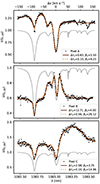 |
Fig. A.1. Degeneracy between the scaling factor β and the optical depth Δτ. The figure shows the intensity profiles for the three selected pixels, with two models for each pixel, one with low β and high Δτ, and one with high β and low Δτ. The grey curve is a nearby quiet Sun spectrum. |
All Tables
Retrieved parameters and associated uncertainties using the stacked HAZEL-2 slab model to the observed spectra.
All Figures
|
Fig. 1. Average spectrum and most important spectral lines in the HeSP observations. Black: spatially and temporally averaged HeSP observations. Orange: Atlas profile from Neckel & Labs (1984), arbitrarily scaled to match the continuum of the HeSP data. Solar spectral lines are indicated with dashed vertical lines and telluric water lines with dotted lines. |
| In the text | |
|
Fig. 2. Example HeSP snapshot, at 31 s after the start of the observations. The four groups of four panels display Stokes I (upper left), Q (upper right), U (lower left), and V (lower right). Each group consists of four subpanels, showing an example line profile (upper left), an xλ-slice (upper right), a λy-slice (lower left) and an xy-image (lower right). The locations of the xλ and λy-slices are indicated with blue and red dotted lines in the image, and their intersection is the location for which the line profile is shown. The wavelength of the Stokes Ixy-image in the lower-right is indicated with the orange tick marks in the Stokes I line profile in the upper-left. The Q, U, and V images are wavelength averages, with the average taken over the interval indicated by the orange ticks in the respective frames. The Stokes I intensity is given in arbitrary units. The wavelength axes are specified in units of Doppler velocity relative to λ = 1083.0 nm. An animated version of the figure is available online. |
| In the text | |
|
Fig. 3. Overview of the observed region at 2023-06-29T08:49, the start of the observation. The upper row shows the continuum close to the Fe I 617.3 nm line and the Hα line core. The bottom row shows the line-of sight and plane-of-the-sky components of the photospheric magnetic field, as determined from the spatially-coupled Milne-Eddington inversion of the Fe I 617.3 nm. The red box shows the HeSP FOV and the arrow in the upper left panel points toward solar north. |
| In the text | |
|
Fig. 4. Overview of the HeSP FOV at 246 s after the start of the observations. First row (a–d): magnetic field in the photosphere as determined from a Milne-Eddington inversion of the Fe I 617.3 nm recorded by CRISP. Second row: magnetic field in the chromosphere as determined from the weak-field approximation in the Ca II 854.2 nm (also CRISP data). Bottom two rows: intensity images at various wavelengths. The Hα red wing image is at Δλ = +45 km s−1 from the nominal line core, the Ca II K red wing image at Δλ = +36 km s−1. Panel j shows the intensity normalized to the local continuum intensity I(x, y, λ)/Icont(x, y), the other panels show the unscaled intensity I(x, y, λ). A movie of this figure showing the entire time series is available online. |
| In the text | |
|
Fig. 5. Example He I 1083 nm line profiles that show emission. Left: line profiles. Right: local continuum normalized intensity in the red wing of He I 1083 nm, with the locations of the profiles left indicated with squares of the same color as the profile. The line profiles are taken from the entire time series, not just from the timestep shown in the right-hand panel. The labeled line profiles are discussed in Sects. 5.4–5.6. |
| In the text | |
|
Fig. 6. Emission in pixel A. Upper left: image of the scaled intensity Iλ(x, y, t)/Icont(x, y, t) in He I 1083 nm. Upper-middle: λt-slice of the scaled intensity at the location of the red square in the image. The red tick marks indicate the wavelength and time of the image. Upper right: light curve at the spatial location indicated by the square and the wavelength indicated by the tick marks. The bottom row shows the same for Ca II K, except that the image in the lower-left panel shows Iλ, i.e., it is not scaled to the local continuum intensity. |
| In the text | |
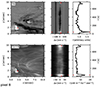 |
Fig. 7. Emission in pixel B. The figure format is the same as in Fig. 6. |
| In the text | |
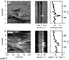 |
Fig. 8. Emission in pixel C. The figure format is the same as in Fig. 6. |
| In the text | |
|
Fig. 9. Inversion results for the three selected pixels with emission in the He I 1083 nm line. The columns show the results for pixels A (left), B (middle), and C (right). The top row shows Stokes I; the bottom row Stokes V. Black-filled circles represent the observations, the orange solid lines are the best-fit profiles. The thin gray curve represents an average of a relatively quiet part of the FOV. |
| In the text | |
|
Fig. 10. Simulation data. Top row: Vertical component of the magnetic field at z = 0 km and emergent intensity at the nominal line core of the strong component of the He I 1083 nm line. Bottom row: zoom in of the region inside the red square in the top row. Panel a: Vertical component of the photospheric magnetic field at z = 0 km; panel b: emergent intensity at the nominal line core of the strong component of the He I 1083 nm.; panel c: local continuum scaled intensity of the He I 1083 nm at a Doppler shift of −18 km s−1; panel d: Hα intensity at a Doppler shift of −33 km s−1; panel e: Ca II K intensity at a Doppler shift of −8 km s−1. The pixel marked with the filled red square is analyzed in Fig. 11. |
| In the text | |
|
Fig. 11. Four-panel formation diagram of the pixel marked in red in the bottom row of Fig. 10. Top left: Opacity χν divided by optical depth τν. The red curve is the height optical depth is unity, the white vertical line marks Δν = 0 and the white curve is the vertical velocity as a function of height. Top right: total source function. The green curve shows the line source function, the orange curve the temperature. Bottom left: τνexp−τν, which peaks at τν = 1. Bottom right: the contribution function χνSνexp−τν. The white curve shows the emergent line profile in temperature units, with a scale on the right. |
| In the text | |
|
Fig. 12. 3D visualization of the magnetic field configuration of the He I 1083 nm emission event in our MURaM simulation. The greyscale background shows the vertical magnetic field in the photosphere (white: positive; black: negative), just above the continuum formation height. The red surface displays the height of optical depth unity z(τ = 1) for the vertically emergent intensity at Δv = −18 km s−1 for the He I 1083 nm line, corresponding to the blue wing images in Fig. 10. This height tends to lie below the height for which we display the magnetic field, and is above it only in some locations, appearing as steeply-sided columns. The magnetic field lines thread the emitting region of the He I 1083 nm brightening, and their color indicates the local temperature. Figure made with VAPOR (Li et al. 2019). |
| In the text | |
|
Fig. A.1. Degeneracy between the scaling factor β and the optical depth Δτ. The figure shows the intensity profiles for the three selected pixels, with two models for each pixel, one with low β and high Δτ, and one with high β and low Δτ. The grey curve is a nearby quiet Sun spectrum. |
| In the text | |
Current usage metrics show cumulative count of Article Views (full-text article views including HTML views, PDF and ePub downloads, according to the available data) and Abstracts Views on Vision4Press platform.
Data correspond to usage on the plateform after 2015. The current usage metrics is available 48-96 hours after online publication and is updated daily on week days.
Initial download of the metrics may take a while.