| Issue |
A&A
Volume 695, March 2025
|
|
|---|---|---|
| Article Number | A193 | |
| Number of page(s) | 23 | |
| Section | Galactic structure, stellar clusters and populations | |
| DOI | https://doi.org/10.1051/0004-6361/202453611 | |
| Published online | 19 March 2025 | |
Signatures of simulated spiral arms on radial actions
1
Université Côte d’Azur, Observatoire de la Côte d’Azur, CNRS, Laboratoire Lagrange,
Bd de l’Observatoire, CS 34229,
06304
Nice cedex 4, France
2
Sydney Institute for Astronomy, School of Physics, A28, The University of Sydney,
NSW
2006, Australia
3
Center of Excellence for All Sky Astrophysics in Three Dimensions (ASTRO-3D),
Australia
4
INAF – Osservatorio Astrofisico di Torino,
via Osservatorio 20,
10025
Pino Torinese (TO), Italy
5
ILANCE, CNRS – University of Tokyo International Research Laboratory,
Kashiwa, Chiba
277-8582, Japan
6
Kavli IPMU (WPI), UTIAS, The University of Tokyo,
Kashiwa, Chiba
277-8583, Japan
7
Sorbonne Université, CNRS, UMR7095, Institute d’Astrophysique de Paris,
98 bis Boulevard Arago,
75014
Paris,
France
8
School of Physics & Astronomy, University of Leicester,
University Road,
Leicester
LE1 7RH, UK
9
Université de Strasbourg, CNRS, Observatoire astronomique de Strasbourg,
UMR 7550,
67000
Strasbourg, France
★ Corresponding author; This email address is being protected from spambots. You need JavaScript enabled to view it.
Received:
25
December
2024
Accepted:
17
February
2025
Abstract
Context. Spiral arms play a key role in the evolution of disc galaxies, defining their morphology, star formation, chemistry, and dynamics. Among their various implications, it has been observed in the Milky Way disc that the distribution of Gaia Data Release 3 (DR3) radial actions exhibits structures that might be related to the spiral arms.
Aims. Our goal is to investigate the relationship between regions of low radial action identified in simulated discs and the location of the spiral arms, such as that suggested for the Galaxy in previous studies.
Methods. For a sample of 23 simulated spiral galaxies, we modelled the axisymmetric component of their gravitational potential to compute the radial action of their stellar particles using the Stäckel fudge. The spatial distribution of the radial action was then compared to the location of the spiral arms, identified as overdensities in the stellar surface density using a kernel density estimator.
Results. Our analysis reveals a strong correlation between the radial action distribution and the spiral arms in 18 of 23 simulated galaxies. However, notable discrepancies are observed in the remaining five, since they are profoundly out-of-equilibrium systems, such as galaxies influenced by external interactions or spiral arms still in the process of winding up. Additionally, spiral arms are consistently traced across young, intermediate, and old stellar populations (≥3 Gyr) in most simulations, suggesting that they are supported by stars spanning a broad age range.
Conclusions. We have confirmed that, in general, there is a tendency for spatial correlation between spiral arms and stellar populations featuring low values of the radial action, as discussed in the literature using Gaia DR3 data. However, discrepancies between features in the radial action distribution and the spiral structure can be interpreted as signatures of recent disturbances, a scenario applicable to the Milky Way. Furthermore, populations at least as old as 3 Gyr trace the spiral arms with no significant misalignment across age bins, suggesting a possible theoretical interpretation of the observations obtained with Gaia data. A linear relation between the maximum value of the radial action of the spiral arms and the vertical scale-length is found, which is also satisfied by the Milky Way.
Key words: Galaxy: disk / Galaxy: evolution / Galaxy: kinematics and dynamics / Galaxy: structure / galaxies: kinematics and dynamics
© The Authors 2025
 Open Access article, published by EDP Sciences, under the terms of the Creative Commons Attribution License (https://creativecommons.org/licenses/by/4.0), which permits unrestricted use, distribution, and reproduction in any medium, provided the original work is properly cited.
This article is published in open access under the Subscribe to Open model. This email address is being protected from spambots. You need JavaScript enabled to view it. to support open access publication.
1 Introduction
Spiral arms are ubiquitous structures in the Local Universe, present in about two-thirds of galaxies (Huertas-Company et al. 2011; Lintott et al. 2011; Willett et al. 2013; Kelvin et al. 2014; Hart et al. 2016, 2017; Masters et al. 2019). This prevalence has facilitated the morphological classification of spiral arms into three categories (Elmegreen & Elmegreen 1982): the ‘grand design’, typically featuring two large, continuous, well-defined arms that complete one revolution around the galaxy; flocculent spiral arms, characterised by a more irregular pattern composed of numerous fragmented segments with no apparent correlation among them (Goldreich & Lynden-Bell 1965; Binney & Tremaine 2008); and a third category comprising intermediatescale arms, whose tracks exhibit bifurcations, branching, and are less extended than the ‘grand design’ arms.
Despite significant research over the last six decades, the formation mechanisms of spiral arms remain unclear, though several models have been proposed to explain these structures. These include the quasi-steady density wave theory (Lindblad 1963; Lin & Shu 1964; Bertin & Lin 1996; Shu 2016), the swing amplification model (Goldreich & Lynden-Bell 1965; Julian & Toomre 1966; Toomre 1981; Grand et al. 2012a,b, 2013; Dobbs & Baba 2014; Michikoshi & Kokubo 2016), transient spiral modes (Sellwood & Carlberg 2014), the dressed mass clump model (Toomre & Kalnajs 1991; D’Onghia et al. 2013), tidal interactions (Toomre & Toomre 1972; Tully 1974; Elmegreen & Elmegreen 1983; Oh et al. 2008; Dubinski et al. 2008; Dobbs et al. 2010), and recurrent cycles of groove modes (Sellwood & Carlberg 2019) among others.
As important drivers of secular evolution (Kormendy & Kennicutt 2004), spiral arms not only define the morphology of galaxies but also contribute to the redistribution of angular momentum (Lynden-Bell & Kalnajs 1972; Minchev & Famaey 2010; Minchev et al. 2011), the heating of the disc (Martinez-Medina et al. 2015; Grand et al. 2016), radial migration (Sellwood & Binney 2002; Di Matteo et al. 2013), and the thickening of the disc (Roškar et al. 2013), to cite a few examples. Therefore, the presence of spiral arms has implications for disc kinematics and dynamics. In contrast to face-on external galaxies, where the presence of the spiral structure can be detected by direct imaging, our position within the Galactic disc complicates the detection of the Milky Way’s spiral arms by this technique, requiring more indirect methods such as those based on distributions of young objects (Reid et al. 2014, 2019; Xu et al. 2018, 2021a,b; Pantaleoni Gonzάlez et al. 2021; Zari et al. 2021; Gaia Collaboration 2023b,a; Ge et al. 2024; Rezaei et al. 2024), chemistry (Poggio et al. 2022; Spitoni et al. 2023; Hawkins 2023; Barbillon et al. 2025; Hackshaw et al. 2024; Debattista et al. 2025), kinematics (Antoja et al. 2011; Hunt et al. 2015; Martinez-Medina et al. 2022; Denyshchenko et al. 2024), and dynamics (Trick et al. 2017; Hunt et al. 2019; Sellwood et al. 2019; Palicio et al. 2023; Khalil et al. 2024). Sellwood et al. (2019) performed a detailed analysis of the Gaia Data Release 2 (DR2) dynamics (Gaia Collaboration 2018) in the very solar neighbourhood (~200 pc from the Sun) to test some of the spiral arm models mentioned above, concluding that the dressed mass model is favoured. Mata-Chávez et al. (2019) studied the relation between the physical parameters of simulated spiral arms with their formation mechanisms, although they did not perform a comparison with those of the Milky Way.
Using the full kinematics sample from Gaia DR3 (Gaia Collaboration 2023c), in Palicio et al. (2023) we mapped the radial actions, JR, and identified areas in the Galactic disc characterised by low values of JR compared to the whole explored region. The location and shape of most of these areas were compatible with those believed to trace spiral arms identified using young tracers such as masers (Reid et al. 2014), upper main sequence stars (Poggio et al. 2021), and Cepheids (Lemasle et al. 2022). This correlation can be attributed to the fact that stars are believed to form on nearly circular orbits within spiral arms, resulting in low radial actions. Although satisfactory, we could not completely rule out the contribution of moving groups to the features seen in the JR maps, and some discrepancies were observed in the IV quadrant (−90° < ℓ < 0°). Our results also suggested that older populations can support the structure of spiral arms, in alignment with the findings of Lin et al. (2022) and Uppal et al. (2023) concerning the distribution of red clump stars in the Local arm and the Outer arm, respectively.
In this work, we aim to confirm the relationship between spiral arms and regions of low JR , originally reported in Palicio et al. (2023), through numerical simulations. We also address whether older populations can trace spiral arms. This paper is organised as follows. In Section 2, we present the set of simulations used in this work and describe the fitting procedure for the potential and acceleration field. Results and discussions are detailed in Section 3. Conclusions are summarised in Section 4.
2 Simulations
2.1 Selected sample and methodology
We analysed a sample of 23 disc galaxy simulations at redshift zero, comprising seven from the Auriga simulations (Grand et al. 2017, 2024), ten from the Illustris-TNG collaboration (Vogelsberger et al. 2014; Pillepich et al. 2019; Nelson et al. 2019a,b; Pillepich et al. 2024), one from the NewHorizon collaboration (Dubois et al. 2021), and the g2.79e12 NIHAO- UHD simulation (Buck et al. 2020). These simulations represent Milky Way-like galaxies and were selected for the pronounced spiral arms shown in their pre-visualisation images. The galaxies provided by the Auriga, Illustris-TNG, and NIHAO-UHD teams belong to a group or cluster of galaxies and, consequently, their evolution is also affected by interactions with their neighbours, as evidenced by the visualisation of their snapshots. We noted, however, that certain relative isolation criteria were applied to consider them as Milky Way-like candidates, as reported in their respective works. In contrast, the NewHorizon volume was chosen so that most galaxies evolve in a field environment, as does the one selected in this work. Apart from these cosmological simulations, we have considered four controlled simulations of idealised galaxies, two of which were presented in Bland-Hawthorn & Tepper-Garcia (2021) and Tepper-Garcia et al. (2022), respectively, and two unpublished simulations created with the NEXUS framework (Tepper-Garcia et al. 2024). These controlled simulations include the interaction with a point mass intended as a proxy for the Sagittarius dwarf galaxy (Sgr), and differ from one another in their gas content and how it is treated: NEXU S A (cf. Bland-Hawthorn & Tepper-Garcia 2021) is a pure N-body simulation without gas, NEXUS B and NEXUS D (cf. Tepper-Garcia et al. 2022) include an ‘inert’ gaseous disc component with a mass equal to 20% and 10% the total (stars and gas) disc mass, respectively. In these simulations, the gas is treated with a simple isothermal equation of state. Finally, NEXUS C adopts the same initial conditions as NEXUS B, but it includes a prescription for galaxy formation, whereby the gas is allowed to cool and to form stars, accounting for their energetic and mass feedback. We kindly refer to the above mentioned references for more details on each the simulation suites. The nominal resolutions for the baryonic particles, as reported for each family of simulations in their respective works, are: 369 pc (AURIGA), 150 pc (ILLUSTRIS), 34pc (NEWHORIZON), 36 pc (NEXUS), and 265 pc (NIHAO -UHD). The number of stellar particles contained in each simulation, as well as other relevant details, are presented in Table 1.
2.2 Model of the potential
In order to model the axisymmetric component of the gravitational potential, we set the centre of mass of the main galaxy of each simulation at the origin, and rotated the whole system to align the total angular momentum with the vertical axis. For those galaxies that exhibit clumps of accretions in their disc and halo, we manually removed them as their self-gravity constitutes a significant fraction of the potential at that position. By excluding these objects, we avoided the inclusion of misleading local potential values in the fitting process, which are not representative of the global main galaxy’s potential.
We considered three intervals in galactocentric distance, separated at r = rmin and r = rmax, and performed individual fits of the potential in each of them. The primary fit was conducted in the intermediate regime rmin < r < rmax, where most of the features are expected. For this interval, we adopted the series proposed by Hernquist & Ostriker (1992) as fit of our potential Φmid, where
 (1)
(1)
in which
 (2)
(2)
where ξ = (r − a)/(r + a), Pℓ,0 are the Legendre polynomials, and  denotes the Gegenbauer polynomials (Gegenbauer 1884; Abramowitz et al. 1988). The parameter a is a characteristic radial scale length of the disc (McMillan 2017), with values in the range of a few kiloparsecs (~1–5 kpc), to improve the convergence of the series in Eq. (1). The restriction to even values of ℓ in Eq. (1) imposes a vertically symmetric fit between both hemispheres, while the value m = 0 in the associated Legendre polynomial implies no azimuthal variations of Φmid (hence no dependence on the angle ϕ). The coefficients An,ℓ were computed by a least-squared fit of the potential value reported by the simulations, performed over a subsample of randomly selected particles since considering the whole simulation in this procedure is computationally expensive.
Once Φmid is obtained, approximations in the inner (r ≤ rmin ) and outer (r ≥ rmax) region were linked to it. For the inner region, we found good fits for the potential assuming the polynomial form
![Mathematical equation: $\eqalign{ & {\Phi _{{\rm{in}}}}(r,\theta ) = {\Phi _{{\rm{mid}}}}\left( {{r_{{\rm{min}}}},\theta } \right) \cdot \left[ {1 + {a_{00}}u + {a_{12}}u{{\cos }^2}\theta } \right. \cr & \,\,\,\,\,\,\,\,\,\,\,\,\,\,\,\,\,\,\,\,\,\,\,\left. { + {a_{22}}{u^2}{{\cos }^2}\theta + {a_{32}}{u^3}{{\cos }^2}\theta + {a_{24}}{u^2}{{\cos }^4}\theta } \right], \cr}$](/articles/aa/full_html/2025/03/aa53611-24/aa53611-24-eq4.png) (3)
(3)
where u = 1 − r/rmin and the coefficients aij are the free parameters set by the least-square minimisation. For the outer region, we considered a power-law like decay of the potential with distance,
![Mathematical equation: ${{{\Phi _{{\rm{out}}}}(r,\theta )} \over {{\Phi _{{\rm{mid}}}}\left( {{r_{{\rm{max}}}},\theta } \right)}} = {\left[ {1 + {{{{\left( {r - {r_{{\rm{max}}}}} \right)}^2}} \over {R_c^2}}\left( {1 + \left( {{{1 - {q^2}} \over {{q^2}}}} \right){{\cos }^2}\theta } \right)} \right]^{ - \gamma /2}},$](/articles/aa/full_html/2025/03/aa53611-24/aa53611-24-eq5.png) (4)
(4)
where the free parameters are the characteristic radii Rc , the flattening term q, and the index of the power law γ such that Φout ~ r−γ at large distances. Note that both Φin and Φout are continuous with Φmid at r = rmin and r = rmax , respectively. The final model of the potential, Φfit , is obtained by combining the fits across the three distance regimes.
The quality of the potential modelling is illustrated in Figure 1 for a galaxy from each collaboration group, while Figure A.1 shows the corresponding results for the remaining simulations considered in this work. The colour code indicates the most discrepant relative difference between the reported potential and Φfit . With the exception of the galactic centre, most regions of the galaxies show good agreement between the model and the original potential, with values of |Φreal − Φfit| < 0.1|Φreal|, and generally below ~2–3%.
Parameters of the simulations considered in this work.
2.3 Model of the accelerations
The NewHorizon simulation does not directly provide the potential of the stellar particles; instead, it provides their accelerations, a, which relate to the potential via a = −∇Φ. If we assume the potential is axisymmetric, the azimuthal component of the acceleration, aϕ, must be zero. This leaves two components of the acceleration to fit: the radial component, aR , and the vertical component, aZ. Since a single component of the acceleration does not uniquely determine the potential, we need to account for both aR and aZ to estimate the proper Φ(r, θ). Therefore, we assumed a model of the potential given by Eq. (1) and tuned the Anl parameters to minimise
 (5)
(5)
where the summation is performed over NP simulation particles and (R, Z) = (r sin θ, rcos θ) are the cylindrical coordinates. We noted, however, the convergence of Eq. (5) is quite slow, especially at the galactic plane (Kuijken & Dubinski 1995; Dehnen & Binney 1998), so we have added the correction term
 (6)
(6)
in which the free parameters cn improved the least-square minimisation of S2. We also tested a correction similar to that used by Dehnen & Binney (1998) and implemented in GALPY (Bovy 2015) to accelerate the spherical harmonic decomposition; however, Eq. (6) led to lower S2 values.
The resulting fit of the accelerations is illustrated in Fig. 2. As can be seen, the relative errors in the radial acceleration are mostly smaller than 5%, while for aZ these discrepancy can be larger than ±10%. We should note, however, this mismatch is appreciated only at low vertical accelerations (e.g., close to the galactic plane), where the radial forces dominate the dynamics.
For the particular case of the NewHorizon simulation, since no improvement in the fit of a was observed when Φin was considered (see Eq. (3)), we decided to retain Φmid to model the inner galaxy. On the contrary, a potential of the form Φout is used at distances r > 40 kpc.
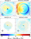 |
Fig. 1 Relative residuals of the potential fits (in percentages) for one simulation from each group considered in this work. The cells show the most extreme relative discrepancy between the model and the nominal potential reported in the simulation within the range |Z| < Zlim. The black cross in the lower-left corner indicates the scale of ±10 kpc. The corresponding maps for the other simulations can be found in Figure A.1. |
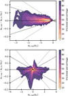 |
Fig. 2 Model of the accelerations of the NewHorizon simulation. Upper (lower) panel: discrepancy between the reported radial (vertical) acceleration and its fit as a function of the acceleration itself. The colour-bars indicate the percentage of stellar particles enclosed in each region. Dashed (dotted) lines represent relative errors of ±5% (±10%). All the accelerations are expressed in units of a⊙ ≈ 6895.6 km2 s−2 kpc−1. |
2.4 Spiral arm overdensities
In order to identify the spiral arms, we applied a bivariate kernel density estimator (KDE) technique similar to that exploited by Poggio et al. (2021). Using this approach, at the location (X, Y) we approximate the local surface density, Σ(X, Y; h), as
 (7)
(7)
where K(x; h) ~ (1 − x2/h2) if |x| < h is the Epanechnikov kernel function, which weights the contribution of a particle at distance |x| to the density at origin, assuming a characteristic bandwidth h (Epanechnikov 1969). For distances |x| > h, the Epanechnikov kernel is zero. The summation in Eq. (7) is performed over all the particles located at (xi, yi) with mass mi. Analogously, the global surface density, Σ(X, Y; H), is estimated as its local counterpart by using a bandwidth H > h, so that the contrast density, δΣ , is determined by their relative difference as
 (8)
(8)
The selected values for h and H for each simulation are summarised in Table 1. The parameter h is set to approximately match the width of the spiral arms, whereas H represents the typical range of large-scale density variations in the disc.
Figures 3, B.1–B.4 illustrate the maps of δΣ(X, Y) for each simulation in the region |Z| < Zlim (values in Table 1). In most simulations, the distribution of δΣ is influenced by short-scale distortions, particularly in the outer regions of the galactic disc, where the effects of Poissonian noise become more pronounced due to the low density in these areas. We reduced the contribution of such fluctuations by reconstructing δΣ (X, Y) from its truncated Fourier series approximation as
![Mathematical equation: ${{\tilde \delta }_\Sigma }(X,Y) = \sum\limits_{n = 0}^{11} {\sum\limits_{m = 0}^{11} {{C_{n,m}}} } \exp \left( {{{2\pi i} \over {{L_{{\rm{kpc}}}}}}[n \cdot X + m \cdot Y]} \right),$](/articles/aa/full_html/2025/03/aa53611-24/aa53611-24-eq10.png) (9)
(9)
where Cn,m are the coefficients of the Fourier expansion of δΣ and Lkpc denotes the limits of the square maps shown in Figs. 3, B.1–B.4. Thus, by approximating δΣ by  (second columns in Figs. 3, B.1–B.4), we are able to reduce the noise and enhance the larger scale structures in the contrast density maps.
By observing the maps of δΣ and  , we visually identified the tentative trace of the spiral arms (dotted lines in the Figures) for sake of comparison with the features in JR. The criteria for considering these features as part of the spiral arms depend on: (i) their extent, where segments significantly larger than their width are readily accepted; (ii) its location, as features in the less dense outer regions require special attention due to the Poissonian noise in the δΣ maps or from artefacts caused by the periodic boundaries of
  , a natural consequence of the Fourier reconstruction; and (iii) the degree of agreement between
  , where, if the previous criteria are not enough to accept a feature, we check whether its inclusion is consistent with the extension of other nearby structures. Since these criteria rely on visual inspection of the reported maps, some minor or ambiguous features may have been omitted. However, none of these omissions are expected to significantly affect the overall spiral pattern of the galaxy, which is dominated by the large, clearly discernible structures usually located at R < Lkpc .
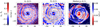 |
Fig. 3 Maps of the density contrast (first column), its bidimensional Fourier approximation (second column), and mass-weighted median radial action (third column) for the AURIGA 2 simulation. Open circles in second and third panels denote the inferred tracks for the spiral arms. The corresponding maps for the rest of simulations considered in this work can be found in Figs. B.1–B.4. |
2.5 Computation of the radial actions
For each simulation, we estimated the orbital parameters, actions and energy by using the potential Φfit (see Section 2.2) in the code used in Palicio et al. (2023) instead of the Galactic potential of McMillan (2017). Assuming an axisymmetric potential, this code implements the Stäckel-fudge approximation method (Famaey & Dejonghe 2003; Binney 2012; Sanders & Binney 2016; Mackereth & Bovy 2018; Bland-Hawthorn et al. 2019; Hadden 2024, but see also Appendix B of Palicio et al. 2023) to estimate the apocenter, pericenter, eccentricity, maximum galactic height and actions from the input position and kinematics.
The maps of the radial action, JR , can be seen in the rightmost columns of Figs. 3, B.1–B.4. In contrast to Palicio et al. (2023), where the number of Gaia DR3 stars exceeded that of particles in our simulations, we had to consider an Epanechnikov kernel with h = 0.5 kpc to effectively increase the number of particles per cell1 in the maps of JR . The contribution of each particle to the median JR within a cell is weighted by its stellar mass.
3 Results and discussions
3.1 Radial action of the spiral arms
The maps represented in the first columns of Figures 3, B.1–B.4 illustrate the contrast of stellar mass density, δΣ, among the different regions of each galaxy. In these panels, we can discern several arc-shaped structures whose densities exceed those of their surroundings (red areas), which we identify as the loci of the spiral arms. They are oriented around the galactic centre, with some bifurcating (as those in AURIGA 2 and AURIGA 3, for example), having kicks in their pitch angles (e.g., AURIGA 16 and AURIGA 24) or showing distortions due to remnants of accreted satellites (e.g., ILLUSTRIS 532760). The contrast density maps filtered for short-scale features,  , are shown in the middle columns of Figs. 3, B.1–B.4, and are adopted as a visual reference for exploring the noisy regions, in which we traced, by visual inspection, those over-density structures that we attributed to the spiral arms (dotted curves in Figs. 3, B.1–B.4). Conversely, we excluded the inner galaxy from our analysis since the high mass of the bulge biases the δΣ estimator there, leading to unrealistic values of the density contrast (blue annular regions at origin in left and middle columns of Figs. 3, B.1-B.4). Similarly, we did not consider as representative of the main galaxy morphology the features in δΣ created by remnants of accreted satellites, as those seen, for example, in ILLUSTRIS 424288 at (Χ,Υ)≈(−24.5, 9.0), (5.1, −25.0), and (21.0, 17.0) kpc.
The spatial distribution of the median radial action (right columns) also reveals arc-shape structures that trace the low JR regions. In contrast to those in δΣ , whose width typically ranges between ~1.5 and ~2.5 kpc, the features in JR can be up to ~4–5 kpc width (e.g., AURIGA 16 and ILLUSTRIS 555287). By confronting the maps of δΣ and median JR , we find the overdensities of stellar mass tend to be located at the low radial action areas (dotted curves in middle and right columns), although noticeable discrepancies are observed both in the external zones (e.g., AURIGA 24, ILLUSTRIS 549516, and NEXUS A) and the central regions (e.g., ILLUSTRIS 42428 8).
To evaluate the quality of correspondence between the high δΣ and the low radial action arcs, we examined the value of JR at the location of the nodes that indicate our estimation of the spiral arm tracks (i.e., the circles that form the dotted curves in Figs. 3, B.1–B.4). The separation between two consecutive nodes is 2 kpc. subsequently, these nodes are classified into three categories based on the degree of agreement with JR : category ‘G’ (good) for the cases in which the δΣ-JR correlation is clear, ‘F’ (fair) if a correspondence exists between the features in δΣ and JR despite some mismatch, and ‘B’ (bad) ifno agreement is observed. specifically, the criteria for category ‘F’ include cases that would align after shifts of ≾1 kpc in their position, a natural extension of their arcs, or are located in a slightly elevated JR area (light bluish areas in the map of the median JR). As an illustrative example of this intermediate category, in ILLUSTRIS 424288, six of the seven last nodes of the spiral arm that ends at (X,Y)≈(15.3, 0.5) kpc were classified as ‘F’ nodes. Another example can be found in the nodes between (X, Y)≈(5.0, 20.), and (10.0, 23) kpc in ILLUSTRIS 549516, since their median JR is slightly above the border value (0.02 L⊙) and they bridge the extremes of the arc feature they belong to.
Due to the difference in the width of the arcs seen in the δΣ (or  ) and JR mapss, as well as the Poissonian noise in the outer regions (usually at R ≿ Lkpc), a correlation diagram of δΣ vs. JR does not clearly show the connection between the overdensities and the zones of low radial action. However, we present these diagrams in Appendix C where, despite the large scatter, all the simulations show an anticorrelation between δΣ and JR .
The resulting classification revealed the nodes tagged as ‘G’ constitute, on average, the 62.6% of the total nodes of a simulation. This percentage, however, ranges from 14.7% for the NEXUS A simulation to 88.1% for AURIGA 16, while 18 of the 21 galaxies have percentages for the ‘G’ sample ≿50%2. If we consider the combination of categories ‘G+F’ as positive matches, the percentage of agreement rises, on average, to 80.2%; while all the simulations exceed the 70% threshold but two: NEXus A (57%) and AuRIGA 2 (67%). The percentage of agreement for each galaxy is indicated in Table 2.
3.2 Anomalous scenarios
Although most of the spiral arms analysed above show a correlation with the low JR regions, we have detected a few discrepancies in some cases, especially in the NEXus family of simulations, as well as in other numerical galaxies not included above but described and discussed as follows. In the first panel of Fig. B.4, we can observe a misalignment between the spiral arms, as traced by the overdensity in δΣ , and the low JR regions for the NEXus A simulation. This mismatch is more evident at the outermost parts (R ≿ 20 kpc) of the main spiral arms of NEXus A, NEXus C, and NEXus D (first, third, and fourth panels in Fig. B.4, respectively); as well as in the innermost ~10 kpc where the spirals wind up bringing closer the features in JR . We interpreted these mismatches as a consequence of a configuration far from the equilibrium for these simulations, as evidenced by the void in the inter-arm region at Y ≿ 20 kpc. Furthermore, we verified the radial velocity field, VR, suggests an eventual wind up of the major arm there, removing the gap and leading to a more relaxed configuration. The same argument applies in the R ≾ 10 kpc regions, where the particles in the arm (inter-arm) show inwards (outwards) radial motions. In other words, the spatial shifts observed between the high density and the low JR areas are compatible with a spiral pattern that is still winding up.
Other major discrepancy concerns the spiral arm detected at the lowermost boundary of the above mentioned gap; such as that starting at (X, Y) ≈ (28, 0) kpc in NEXus A but with analogous examples in all the NEXus simulations. This spiral arms do not lie on a low radial action area but trace the envelope of the highest JR region. Although the out-of-equilibrium scenario described above can explain such discrepancy with the other simulations, there is an alternative explanation for such mismatch concerning the kernel technique described in sect. 2.4: the abrupt transition from moderately populated (i.e., region below the dotted curve starting at X=20 kpc, Υ=0 kpc) to almost empty areas (above the dotted curve) can produce misleading estimations of the density contrasts, which might be misinterpreted as spiral arms. This idea is explained in detail in Appendix E.
In addition to the AURIGA simulations presented in Figs. 3 and B.1, we analysed the peculiar case of AURIGA 23, whose overdensity map (upper-left panel in Fig. 4) suggests the presence of a long bar in the central regions. As commonly done in the literature (e.g., Martinez-Valpuesta et al. 2017; Thomas et al. 2023; Bland-Hawthorn et al. 2024), we used the ratio between the amplitudes of the dipolar A2 and the axisymmetric A0 components of the surface density to confirm the existence of the bar and quantify its strength. We computed A2 /A0 over the range R = 0.5 to 7.5 kpc using bins of ΔR = 0.5 kpc width with a 50% overlap.
As shown in Fig. 5, AURIGA 23 exhibits a large A2 /A0 ratio (~0.4) compared to most of the simulations, surpassed only by AURIGA 24 (A2/A0 ≈ 0.54), two earlier snapshots of AURIGA 23 from ~3 Gyr and ~1 Gyr ago (A2/A0 ≈ 0.53 and ≈0.41, respectively), and ILLUSTRIS 552414 (A2/A0 ≈ 0.52) with a ~2 kpc half-length bar. Despite being stronger, the bars in AURIGA 24 and ILLUSTRIS 552414 do not seem to cause significant distortions in the distribution of radial actions. To explore this in detail, we located the resonances associated with the m = 2 and m = 4 perturbers of these galaxies and checked whether the radial action maps show any imprint of them at these positions. In particular, when two perturbers with different pattern speeds coexist, an overlap of their resonances can induce a significant exchange of angular momentum (Quillen 2003; Minchev & Famaey 2010; Minchev et al. 2011) in a nonlinear fashion (i.e., the effect of the combined perturbers exceeds that produced by each of them individually) – especially if the bar’s corotation or outer Lindblad resonance is involved. This change in angular momentum would imply a variation in the radial action whenever a resonance other than corotation participates (Sellwood & Binney 2002), as suggested by the increase in the radial velocity dispersion reported by Minchev & Famaey (2010).
Therefore, for the AURIGA 24 and ILLUSTRIS 552414 galaxies, we located the resonances of their m = 2 and m = 4 per- turbers, estimating their pattern speeds through the 2D Fourier mode velocity method (Pfenniger et al. 2023). We noted that, due to the complexity of the structures in the discs of simulated galaxies-where multiple perturbers can coexist with different pattern speeds and transient behaviour–the inferred rotation Ω and epicyclic κ frequencies may not decrease monotonically with radius. Consequently, a galaxy may exhibit more than one outer Lindblad resonance, as is the case for AURIGA 24 and ILLUSTRIS 552414.
As Figure 6 illustrates, the AURIGA 24 simulation shows three resonance overlaps created by the m = 2 and m = 4 modes (hereafter denoted by the subscripts ‘b’ and ‘s’, respectively): an overlap between the corotation resonances at RCR,b ≈ RCR,s ≈ 3.0 kpc, and two overlaps involving the 2 : 1b, 2 : 1s, and 4 : 1s resonances at ~5.75 kpc and 16.5 kpc. Among them, only the corotation overlap appears to have a significant impact on the radial action distribution, acting as a barrier for the innermost low-JR regions.
Conversely, in the ILLUSTRIS 552414 simulation, the corotation radii RCR,b and RCR,s are slightly more separated, while the 2 : 1b resonances overlap with the ultraharmonic 2 : 1s and the outer Lindblad resonances 4 : 1s at 5.5, 8.5, 10.5, and 16.5 kpc. However, we detected no distinct features in the JR distribution that suggest any influence from these overlaps, except for limiting the innermost low-JR regions at the corotation radii, similar to AURIGA 24. In contrast to AURIGA 24 and ILLUSTRIS 552414, the AURIGA 23 snapshots reveal two crescent-shaped regions of low JR located on either side of the bar’s minor axis, indicating a notable impact on the radial action distribution in this area.
Finally, the analysis of the ILLUSTRIS 456326 simulation revealed a significant mismatch between the overdensities in δΣ and the features in the median JR (Fig. 7). The latter exhibited very extended structures compared to those observed in the other simulations. To evaluate the reasons behind these discrepancies, we explored the recent history of this simulation using earlier snapshots. 1.35 Gyr ago, the spiral arms of ILLUSTRIS 456326t91 showed a strong correlation with the low-JR regions, representing one of the clearest examples in our study. This agreement persisted until snapshot ILLUSTRIS 456326t94, corresponding to 0.9 Gyr ago, where a ring-shaped area of low radial action emerged at R ≈ 6.5 kpc, and slight misalignments between the spiral arms and the arcs in JR became noticeable.
At later times, the maps from subsequent snapshots reveal a new configuration of the overdensities in δΣ , which reorganised to eventually form two large spiral arms. Meanwhile, the ring-shaped low-JR area expanded to R ≈ 10.8 kpc in snapshot ILLUSTRIS 456326t95 (0.7 Gyr ago). In the following snapshots, there is a complete misalignment between the overdensities and the arcs in JR , with no discernible patterns emerging. At the present time, the ILLUSTRIS 456326 simulation shows two banana-shaped regions characterised by low radial action, of which only the uppermost region includes a spiral arm.
We interpreted the evolution described above as the result of an interaction between the main ILLUSTRIS 456326 galaxy and a nearby satellite, whose mass comprises 20% of the total system’s mass. The pericenter of this encounter was located, at most, at 44.2 kpc (snapshot ILLUSTRIS 456326t95) from the centre of the main body, producing an overlap between the discs of both galaxies approximately ~0.7 Gyr ago. The effects of this interaction can be observed in Fig. A.2, where the companion caused significant distortions and asymmetries in the potential of the main galaxy.
statistics of the node classification based on the agreement between the δΣ overdensity and the low JR regions.
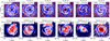 |
Fig. 4 Maps of the density contrast (upper panels) and mass-weighted median radial action (bottom panels) for the AURIGA 23 barred simulation analysed in Section 3.2. Open circles denote the inferred tracks for the spiral arms. |
 |
Fig. 5 Absolute value of the dipolar-to-axisymmetric component of the density ratio, |A2/A0|, for all the simulations considered in this work. Large values of A2 /A0 denote great contribution from elongated structures, like a bar, to the local density. For the sake of visualisation, the complete set of simulations has been divided into five panels. |
 |
Fig. 6 Location of the resonances created by the m = 2 and the m = 4 perturbers in the AURIGA 24 and ILLUSTRIS 552414 simulations. Blue (red) vertical lines refer to the m = 2 (m = 4) perturber; while the linestyle denotes the frequency ratio involved: corotation (solid lines), first harmonics 2 : 1b and 4 : 1s (dashed lines), second harmonics 1 : 1b and 2 : 1s (dotted lines). |
3.3 Age of the spiral arm population
Apart from the low JR-overdensity correspondence, the results of Palicio et al. (2023) suggested the spiral arms might be also supported by populations older than expected. In that work, we were able to discern the spiral arms in the distribution of JR using a photometrically selected sample of Gaia DR3 giant stars. Furthermore, by reproducing the KDE technique described in Sect. 2.4, we observed overdensities of giant stars at the locations of the spiral arms reported by Poggio et al. (2021) and traced by upper main sequence stars. The idea of old populations contributing to the spiral arm structure is not new but was originally noted by Zwicky (1955) and Schweizer (1976), although for ‘grand design’ spirals (Eskridge et al. 2002). However, the spiral arms of the Milky Way are thought to be intermediatescale or flocculent types (Binney & Tremaine 2008; Quillen et al. 2018; Martinez-Medina et al. 2022), and they are not expected to be long-lived structures (Oort 1970; Elmegreen & Elmegreen 1984).
The methodology of Palicio et al. (2023), however, offers an alternative explanation for the features seen in their JR maps with giants stars: their uncertainties in the photometric selection criteria (observational errors, incorrect estimation of the extinction, etc.) may have misclassified some young sources as giants, in which the former would be preferentially located at the spiral arms regions they were born. On the contrary, the giant population would show a more uniform spatial distribution since it is older. Although the polluting young sample were smaller in volume compared to the old one, the KDE method would enhance the spatial asymmetries of the former revealing the spiral arms.
In order to address whether the old population can trace the spiral arms or not, we have applied the KDE technique on three subsets of different ranges of age, τ: the young (τ ≤ 1 Gyr), intermediate (1 ≤ τ < 2 Gyr) and old (2 ≤ τ < 3 Gyr) populations. The resulting maps for δΣ are illustrated in Figs. 8, D.1–D.3. In general, all the spiral arms traced by the whole simulation (dotted lines) are observed at the three age intervals, although a few minor discrepancies are found in ILLUSTRIS 464163, where half of the spiral arm starting at (X, Y) ≈ (1.4, –10.4) kpc is not traced by the oldest sample; in ILLUSTRIS 479290, where the small overdensities at the upper right corner of the maps can be only identified in the young subset; as well as in NEWHORIZON, in which the most external spiral arms are not discernible in populations older than 1 Gyr. In contrast, the spiral arms of the NIHAO-UHD simulation are almost exclusively supported by the young population.
Our results align with the findings of Lin et al. (2022) and Uppal et al. (2023), who demonstrated that it is possible to trace the Local and Outer spiral arms, respectively, using the red clump population, whose age distribution is expected to peak at ~1–4 Gyr (Girardi & Salaris 2001; Girardi 2016). Similarly, Khanna et al. (2024) identified structures in the distribution of red clump stars consistent with the spiral arms traced by Drimmel (2000), although none correspond to the Local Arm. In a recent study, Debattista et al. (2025) identified the spiral arms of their simulated galaxy by analysing the population older than 2 Gyr.
We do not observe, however, any significant misalignment in the spiral arm traces across the three age bins (Rand & Kulkarni 1989). This contrasts with the findings of Hao et al. (2021), who reported offsets using masers and young open clusters. A key distinction is that their oldest age interval extends up to 0.1 Gyr, whereas our youngest age bin is an order of magnitude greater. Consequently, it is likely that our maps lack the resolution necessary to disentangle the offsets between populations of such small age difference.
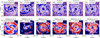 |
Fig. 7 Maps of the density contrast (upper panels) and mass-weighted median radial action (bottom panels) for different snapshots of the ILLUSTRIS 456326 simulation, which is affected by a recent merger, as analysed in Section 3.2. Open circles denote the inferred tracks of the spiral arms. |
 |
Fig. 8 Density contrast maps of the AURIGA 2 simulation for three distinct age intervals: stellar particles younger than 1 Gyr (left column), those aged between 1 and 2 Gyr (middle column), and those between 2 and 3 Gyr (right column). Open circles indicate the spiral arm tracks inferred from Fig. 3. Cross in the bottom-right corner indicates the scale of ±5 kpc. |
3.4 Relation to the Milky Way
The arc-shaped structures identified in the maps of radial actions are not delimited by a single value of JR common to all the simulations. Instead, each galaxy requires an individual reference value, JR,w , that separates the high and low radial action regions (see rightmost colour-bars in Figs. 3, Β.1–Β.4). Motivated by the results of Jia et al. (2023) and Jia et al. (2024), who identified a correlation between the vertical scale-length, hZ, and the mean radial action along the disc of the form JR ~ (hZ – b)2, we investigated a potential connection between JR,w and the vertical and radial (hR) scale-lengths. These parameters are represented on the horizontal axis of Fig. 9.
The scale-lengths hR and hZ were computed assuming exponential fits for the histograms of stellar masses along the radial and vertical directions, respectively. Since the discs of the analysed simulations show non-negligible deviations from exponential profiles in the radial direction, we considered the average of two estimations for hR : one imposing R < Lkpc and another with R < Lkpc/2 as the maximum galactocentric distance for the histogram. In both cases, the criteria |Z| < Zlim and 0.2Lkpc ≤ R were applied to focus on the galactic plane and exclude the bulge regions, respectively. Similarly, for hZ, we averaged the estimations within |Z| < Zlim and |Z| < Zlim/2, imposing 0.2Lkpc ≤ R < Lkpc . The discrepancy between both estimations is denoted by the (symmetric) error bars in Fig. 9.
As shown in the upper panel of Fig. 9, no clear trend JR,w(hR) can be inferred from the distribution of data points, primarily due to the large errors associated with the estimation of hR . Its vertical counterpart, however, shows a positive correlation between the radial action JR,w and hZ . To confirm this correlation, we performed a linear fit excluding outliers through a σ-clipping procedure: in each iteration, only the data points whose absolute discrepancy lay within the 75th percentile participated in the next fit (filled markers in Fig. 9). The resulting parameters of the fit confirmed our visual interpretation of the JR,w vs. hZ correlation, showing a positive slope of 3.69 × 10⁻² L⊙/kpc. This correlation is analogous to that found by Jia et al. (2023) at different ranges of Galactocentric radii, although we adopted a simpler functional form for the fit. Jia et al. (2023) proposed a parabolic fit for JR,w (hZ), as predicted by some distribution functions for the Milky Way under the epicycle approximation (see Problem 4.21 in Binney & Tremaine 2008), while we found that a linear relation provides an adequate fit to the data points. It is important to note, however, that the parameter JR,w does not correspond to the mean radial action as in Jia et al. (2023), and we did not subdivide the data into radial bins as they did. Consequently, the observed trends of JR,w with scale lengths or velocity dispersions might appear linear rather than quadratic.
For comparison with the Milky Way, we included estimations for hR and hZ in the diagrams of Fig. 9 (black markers3). We adopted the value JR,w = (9.4 ± 0.6) × 10−3L for the Milky Way from Figure 1 of Palicio et al. (2023), while those for hR were extracted from the compendium presented in Bland-Hawthorn & Gerhard (2016). For the vertical scale length, we considered hZ ≈ 0.3 kpc, as widely reported in the literature for decades (Gilmore & Reid 1983; JuriJurić et al. 2008).
The large error bars associated with the radial scale-length estimates prevent reliable comparisons, in which the Milky Way’s hR remains the shortest among them. Conversely, the position of the Milky Way in the JR,w vs. hZ plane aligns with expectations from the linear fit, as well as with those of the NEXUS galaxies.
As noted by Jia et al. (2023), the correlation between hZ and the radial action can be explained as a consequence of the disc’s underlying heating mechanisms, which broaden the distribution of radial actions and increase the velocity dispersions. This implies greater kinetic energy in the vertical direction, allowing stars to reach larger galactic heights. Since radial actions are always positive, the broadening of the JR distribution is associated with a shift of the mean and median towards higher values. This effect can be visualised assuming an exponential distribution for JR, as in Fig. 3 of Jia et al. (2023), where the mean and median are proportional to the scale factor. We attribute the lack of correlation between JR,w and hR to their evolution through different mechanisms: the radial action is a key parameter determining the orbital eccentricity, ecc, around the Galactic centre ( under the epicyclic approximation, as shown in Eq. 3.261 of Binney & Tremaine 2008). Thus, increasing the radial action implies larger ecc, leading to an outward displacement of the apocenter4, rapo . In this configuration, stars can visit outer disc regions, which might suggest, erroneously, that hR has increased due to stellar mass being pushed outward. However, larger eccentricities also imply shorter galactocentric distances for the pericenter, resulting in stellar mass transport towards central regions and a reduction of the radial scale-length. Consequently, changes in radial action induced by heating mechanisms are unlikely to significantly impact hR, particularly within the epicyclic approximation regime. However, when this approximation does not hold, as in the case of very eccentric orbits, a star may spend more time at galactocentric distances greater than its guiding radius than within it. This implies, on average, a net outward displacement of mass. In contrast, changes in angular momentum, LZ , directly affect the guiding radii of the orbit, a proxy for the mean galactocentric distance, potentially triggering radial migration that redistributes mass outward, thereby increasing hR. In alignment with this interpretation, Frankel et al. (2020) reported changes in the angular momentum of the Milky Way thin disc that are approximately 10 times larger than those in radial action. In a recent study, Hamilton et al. (2024) explored several models of spiral arms to reproduce the observed heating- to-migration ratio of ~0.1. They concluded that the non-linear horseshoe transport mechanism (Sellwood & Binney 2002) is compatible with the observations, albeit under rather specific conditions related to the spatial extent of the perturbation amplitude or the presence of greater pitch angles in the past. However, in the former scenario, the non-horseshoe scattering mechanism can also be consistent with the data.
It is interesting to compare the radial action maps presented in this work to the one obtained for the Milky Way, represented in Fig. 1 of Palicio et al. (2023). In our Galaxy, however, the comparison between the JR maps and the spiral structure is not trivial, because there is no consensus about the geometry and number of spiral arms in the Galactic disc. Low-JR features from Palicio et al. (2023) tend to be co-located with the spiral arm geometry proposed by Reid et al. (2014), with the exception of the Scutum arm and a small part of the Perseus arm in the third Galactic quadrant (see second panel of Fig. 4 in Palicio et al. 2023). The general good agreement between the spiral arm model from Reid et al. (2014) and the observed low-JR features would suggest a connection between the two, as seen in the majority of the simulated galactic discs analysed in this work.
However, a larger pitch angle for the Perseus arm has been found by other works based on young stars in Gaia (Zari et al. 2021; Poggio et al. 2021; Gaia Collaboration 2023a) and Cepheids (Drimmel et al. 2025), in agreement with the model by Levine et al. (2006) based on HI observations (see their spiral arm no. 2). Such pitch angle would also be consistent with the map obtained with the giant sample in Palicio et al. (2023). Assuming the Perseus arm geometry from these works, the low-JR feature in the outer disc mapped by would not coincide with a spiral arm (see first and last panels of Fig. 4 in Palicio et al. 2023). Therefore, in this scenario, the outer disc of the Milky Way would be more similar to the out-of-equilibrium simulated galaxies analysed in this work (Antoja et al. 2018; McMillan et al. 2022; Poggio et al. 2024); although similar discrepancies have also been observed in less disturbed simulations.
Based on all spiral arm geometries explored, the structures tentatively associated with the Local and Perseus spiral arms, respectively, merge in an area of low JR, showing a certain misalignment with the literature – except for the 17th group of Cepheids reported in Lemasle et al. (2022). By analysing the maps for δΣ and JR from the simulations, we identified similar structures, where the region between two nearby spiral arms also presents low radial action. This is the case for the bifurcation at (X, Y) ~ (-8,0) kpc in AURIGA 19 (third row in Fig. B.1), at (10, -6.6) kpc in AURIGA 27 (fifth row in Fig. B.1), at (−5.3, −7.3) kpc in ILLUSTRIS 555287 (fourth row in Fig. B.3), and the gap between two spiral arms in NEXUS D at (10.6,0) kpc (fourth row in Fig. B.4). While reaching a definitive conclusion about the Milky Way remains challenging, there is no doubt that mapping JR features in the Galactic disc provides a unique perspective on the dynamical history of the Galaxy, as demonstrated by the simulations analysed in this work.
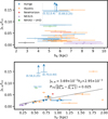 |
Fig. 9 Dependence of JR,w with the structure and kinematic parameters of the simulations: radial scale-length (upper panel) and vertical scalelength (lower panel). Coloured markers refer to simulation families: AURIGA (blue circles), ILLUSTRIS (orange triangles), NEWHORIZON (red diamond), NEXUS (purple triangles), and NIHAO-UHD (green square). Black markers denote measurements for the Milky Way reported in the literature (see main text). Open markers denote outliers excluded from the linear fit (dashed line) by the σ-clipping algorithm. |
4 Conclusions
Our analysis of a set of simulations from independent groups supports the correlation between the location of the spiral arms and the low radial action features, as proposed by Palicio et al. (2023) using Gaia eDR3 and DR3 data (Gaia Collaboration 2021, 2023c). In that work, the features in JR were mainly consistent with the models of the Sagittarius, Local, and Perseus spiral arms proposed by Reid et al. (2014) in the first and second quadrants (0° ≤ ℓ ≤ 180°), while at negative longitudes, no preferential model emerged from the comparison with the literature. For our sample of simulations, such correspondence was observed in 20 of the 23 spiral galaxies, with an average percentage of agreement ranging from the 64% to the 88.1%, depending on the strictness of the goodness criterion. Conversely, for the remaining two simulations, the mismatch between the δΣ and the JR maps can be explained by an out of equilibrium state, such as that triggered by an interaction with a companion galaxy (ILLUSTRIS 456326, NEXUS A-D), and by border effects of the KDE technique, as these observed in the NEXUS simulations and explained in Appendix E.
Although restricted to the particular cases of AURIGA 23 and NIHAO-UHD, we found no evidence of a great influence of the bar on the distribution of the radial actions at the locations of the spiral arms. We must exclude from this observation, however, the central regions in which the bar is confined, as two arc-shaped areas of low JR have emerged near the minor axis. In any case, all the conclusions derived for the barred galaxy scenario should be interpreted with caveat since our methodology assumes the potential is predominantly axisymmetric. Therefore, it might result unrealistic if the bar contributes significantly to the total potential, requiring more advanced approaches for the action estimation, such as that proposed by Debattista et al. (2025).
On the other hand, strong interactions with satellites can destroy the existing spiral arm pattern, leading to a new configuration in which the emerging spiral arms do not lie on low JR areas, as observed in the recent history of the ILLUSTRIS 456326 simulation. This perturbed scenario is expected to be transitory and eventually evolve to a new equilibrium state in which the JR-δΣ anticorrelation is recovered. Further re-simulations of post-interaction galaxies are required for confirming this hypothesis.
The maps of the density contrast, δΣ, computed for different bins in age revealed the population older than 1 Gyr can trace the spiral arms. Furthermore, at the spatial resolution of the considered simulations, no significant misalignment among the spiral arm tracks has been observed when compared the three age bins. This contradicts the classical picture of the spiral arms traced by the young sources recently formed in, implying differences in the mean age between the leading and trailing sides of the arms. We recall, however, this contrast in age might not be discernible in our maps due to the spatial resolution. Addressing whether the old population was formed in the spiral arms they are observed in or have been trapped later is beyond the scope of this paper.
The comparison of the limiting value for the low JR regions, JR,w, with the vertical scale-length of the disc reveals a positive correlation between the two, which can be approximated by the linear relation presented in Fig. 9. Given that correlation does not necessarily imply causation, we interpreted that relation as consequence of disc heating, which increases the velocity dispersion raising the eccentricity of the orbits, thereby increasing the radial actions and, consequently, JR,w. On the contrary, no clear trend is observed between the radial scale-length, hR, and JR,w, suggesting that disc heating is not the primary mechanism driving its expansion, although some influence cannot be entirely ruled out.
Acknowledgements
We thank the anonymous referee for their valuable comments, which have helped improve the revision of this manuscript. P. A. Palicio acknowledges the financial support from the Centre national d’études spatiales (CNES). TTG acknowledges partial financial support from the Australian Research Council (ARC) through an Australian Laureate Fellowship awarded to JBH. We have used simulations from the Auriga Project public data release (Grand et al. 2024) available at https://wwwmpa.mpa-garching.mpg.de/auriga/data. The NewHorizon simulation was made possible thanks to computational resources at CINES, TGCC, and KISTI, and local clusters at the Institut d’Astrophysique de Paris and the Yonsei University. This work was granted access to the HPC resources of CINES under the allocations c2016047637, A0020407637, and A0070402192 by Genci, KSC-2017-G2-0003 by KISTI, and as a ‘Grand Challenge’ project granted by GENCI on the AMD Rome extension of the Joliot Curie supercomputer at TGCC. Although GALPY is not explicitly used in this work, P. A. Palicio uses its source code as reference and recognises the credit for the work of Bovy (2015).
Appendix A Maps of the potential fit
As mentioned in Section 2.2, for each simulation we performed a fit of the gravitational potential assuming an axisymmetric formulation for it. The most deviant relative discrepancy between this fit and the potential reported in the simulations is illustrated in Figs. A.1 and A.2.
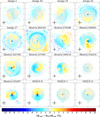 |
Fig. A.1 Relative residuals of the potential fits (in percentages) for each simulation considered in this work. Each cell shows the most extreme relative discrepancy between the model and the nominal potential reported in the simulation within |Z| < Zlim. Black cross in the lower left corner indicates the scale of ±10 kpc. |
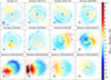 |
Fig. A.2 Similar to Fig. A.1 but for the set of AURIGA 23 and ILLUSTRIS 456326 snapshots used in Section 3.2. Black cross in the lower left corner indicates the scale of ±10 kpc. |
Appendix B Additional maps of density contrast and radial actions
In this section, we present the maps of the density contrasts, δΣ and  , as well as those of the radial actions for the simulations not shown in Figure 3.
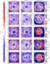 |
Fig. B.1 Maps of the density contrast (first column), its bidimensional Fourier approximation (second column), and mass-weighted median radial action (third column) for a set of simulations not shown in Fig. 3. |
Appendix C The overdensity vs. radial action anticorrelation
As explained in Section 3.1, the difference in the width of the structures observed in the JR maps compared to those in δΣ(X, Y) hinders a clearer discernment of their relationship through visual inspection. This is evident in Figure C.1, where the linear fit, despite significant scatter, shows negative slopes for all the simulations.
 |
Fig. C.1 Distribution of particles in the correlation diagram δΣ vs. JR. The solid lines represent the linear fit of the particle density shown in the background map. The slope of the linear fit is provided in the inset text. |
Appendix D Additional age binned maps of density contrast
In this section, we show the density contrast maps per bin of stellar age, δΣ(X, Y), for those simulations not presented in Section 3.3.
 |
Fig. D.1 Density contrast maps for three distinct age intervals: stellar particles younger than 1 Gyr (left column), those aged between 1 and 2 Gyr (middle column), and those between 2 and 3 Gyr (right column) for a set of galaxies not shown in Fig. 8. Open circles indicate the spiral arm tracks inferred from Figs. B.1–B.4. Cross in the bottom-right corner indicates the scale of ±5 kpc. |
Appendix E KDE technique at discontinuities
In Sect. 3.2, we explained a discrepancy between the δΣ and JR maps, observed in certain regions of the NEXUS simulations, as a misinterpretation of the former as a spiral arm instead of a border effect of the KDE technique. In order to illustrate the mechanisms that produces this effect, we adopted a simplified model of the scenario seen in the simulations in which a medium of constant surface density, Σ0, limits the vacuum at Y = 0. We can obviate the X direction in this approximation. In the neighbourhood of the boundary between the two media, the estimation of δΣ(Y) depends on the distance of the kernel centre with respect to Y = 0 kpc, as well as on the bandwidths h and H used for the local and global KDEs, respectively. Consequently, there are five possible configurations for the relative location of the kernel (upper panel of Fig. E.1). In the configuration labelled as A, the support of the global kernel is completely inside the dense medium. If the support of the local kernel is completely embedded in the dense medium but not that of the global kernel we obtain the configuration B. The configuration C accounts for the partial embedding of both kernel supports, while in the configuration D only that of the global kernel is partially included in the medium. Finally, in the configuration E both kernels do not overlap with the dense medium.
From the mathematical point of view, the generalisation of the KDE technique with continuous media implies the substitution of the summation in Eq. 8 by an integral. Therefore, the local density estimated with the Epanechnikov kernel of bandwidth h is
 (E.1)
(E.1)
where the limits of the integral depend of the configurations shown in Fig. E.1. The estimation of the global density is analogous to Eq. E.1 but replacing h by H. The density contrast δΣ(Y) derived from these estimations is represented in the bottom panel of Fig. E.1 for different distances to the interface, assuming bandwidths of h = 0.5 kpc and H = 2.0 kpc. As can be seen, in configuration B the estimator δΣ is positively biased while at configuration C it may result either positively (peaking at ~0.5 for this example) or negatively biased. Finally, we adopted δΣ = −1 as value for the configuration E to avoid the 0/0 indeterminate form (dashed red line in Fig. E.1).
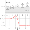 |
Fig. E.1 Visualisation of the border effect produced by the KDE technique on the δΣ map of the NEXUS simulations. Upper panel: scheme of the different configurations of the local (small squares) and global (large squares) scanning windows with respect to the boundary between a medium of uniform density Σ0 (grey area at negative Y) and the vacuum (white region at positive Y). Lower panel: values of δΣ for the mentioned configurations (red curve), assuming h = 0.5 kpc (vertical dotted lines) and H = 2.0 kpc (vertical dashed lines) bandwidths for the local and global kernels, respectively. |
References
- Abramowitz, M., Stegun, I. A., & Romer, R. H. 1988, Am. J. Phys., 56, 958 [NASA ADS] [CrossRef] [Google Scholar]
- Antoja, T., Figueras, F., Romero-Gómez, M., et al. 2011, MNRAS, 418, 1423 [NASA ADS] [CrossRef] [Google Scholar]
- Antoja, T., Helmi, A., Romero-Gómez, M., et al. 2018, Nature, 561, 360 [Google Scholar]
- Barbillon, M., Recio-Blanco, A., Poggio, E., et al. 2025, A&A, 693, A3 [NASA ADS] [CrossRef] [EDP Sciences] [Google Scholar]
- Bertin, G., & Lin, C. C. 1996, Spiral Structure in Galaxies: A Density Wave Theory (Cambridge, MA: MIT Press) [Google Scholar]
- Binney, J. 2012, MNRAS, 426, 1324 [Google Scholar]
- Binney, J., & Tremaine, S. 2008, Galactic Dynamics, 2nd edn. [Google Scholar]
- Bland-Hawthorn, J., & Gerhard, O. 2016, ARA&A, 54, 529 [Google Scholar]
- Bland-Hawthorn, J., & Tepper-García, T. 2021, MNRAS, 504, 3168 [CrossRef] [Google Scholar]
- Bland-Hawthorn, J., Sharma, S., Tepper-Garcia, T., et al. 2019, MNRAS, 486, 1167 [NASA ADS] [CrossRef] [Google Scholar]
- Bland-Hawthorn, J., Tepper-Garcia, T., Agertz, O., & Federrath, C. 2024, ApJ, 968, 86 [Google Scholar]
- Bovy, J. 2015, ApJS, 216, 29 [NASA ADS] [CrossRef] [Google Scholar]
- Buck, T., Obreja, A., Macciò, A. V., et al. 2020, MNRAS, 491, 3461 [Google Scholar]
- Debattista, V. P., Khachaturyants, T., Amarante, J. A. S., et al. 2025, MNRAS, 537, 1620 [Google Scholar]
- Dehnen, W., & Binney, J. 1998, MNRAS, 294, 429 [Google Scholar]
- Denyshchenko, S. I., Fedorov, P. N., Akhmetov, V. S., Velichko, A. B., & Dmytrenko, A. M. 2024, MNRAS, 527, 1472 [Google Scholar]
- Di Matteo, P., Haywood, M., Combes, F., Semelin, B., & Snaith, O. N. 2013, A&A, 553, A102 [NASA ADS] [CrossRef] [EDP Sciences] [Google Scholar]
- Dobbs, C., & Baba, J. 2014, PASA, 31, e035 [NASA ADS] [CrossRef] [Google Scholar]
- Dobbs, C. L., Theis, C., Pringle, J. E., & Bate, M. R. 2010, MNRAS, 403, 625 [NASA ADS] [CrossRef] [Google Scholar]
- D’Onghia, E., Vogelsberger, M., & Hernquist, L. 2013, ApJ, 766, 34 [Google Scholar]
- Drimmel, R. 2000, A&A, 358, L13 [NASA ADS] [Google Scholar]
- Drimmel, R., Khanna, S., Poggio, E., & Skowron, D. M. 2025, A&A, in press, https://doi.org/10.1051/0004-6361/202451100 [Google Scholar]
- Dubinski, J., Gauthier, J. R., Widrow, L., & Nickerson, S. 2008, in ASPC, 396, Formation and Evolution of Galaxy Disks, eds. J. G. Funes, & E. M. Corsini, 321 [Google Scholar]
- Dubois, Y., Beckmann, R., Bournaud, F., et al. 2021, A&A, 651, A109 [NASA ADS] [CrossRef] [EDP Sciences] [Google Scholar]
- Elmegreen, D. M., & Elmegreen, B. G. 1982, MNRAS, 201, 1021 [NASA ADS] [CrossRef] [Google Scholar]
- Elmegreen, B. G., & Elmegreen, D. M. 1983, ApJ, 267, 31 [Google Scholar]
- Elmegreen, D. M., & Elmegreen, B. G. 1984, ApJS, 54, 127 [Google Scholar]
- Epanechnikov, V. A. 1969, Theory Probab. Appl., 14, 153 [Google Scholar]
- Eskridge, P. B., Frogel, J. A., Pogge, R. W., et al. 2002, ApJS, 143, 73 [NASA ADS] [CrossRef] [Google Scholar]
- Famaey, B., & Dejonghe, H. 2003, MNRAS, 340, 752 [NASA ADS] [CrossRef] [Google Scholar]
- Frankel, N., Sanders, J., Ting, Y.-S., & Rix, H.-W. 2020, ApJ, 896, 15 [NASA ADS] [CrossRef] [Google Scholar]
- Gaia Collaboration (Brown, A. G. A., et al.) 2018, A&A, 616, A1 [NASA ADS] [CrossRef] [EDP Sciences] [Google Scholar]
- Gaia Collaboration (Brown, A. G. A., et al.) 2021, A&A, 649, A1 [NASA ADS] [CrossRef] [EDP Sciences] [Google Scholar]
- Gaia Collaboration (Drimmel, R., et al.) 2023a, A&A, 674, A37 [CrossRef] [EDP Sciences] [Google Scholar]
- Gaia Collaboration (Recio-Blanco, A., et al.) 2023b, A&A, 674, A38 [CrossRef] [EDP Sciences] [Google Scholar]
- Gaia Collaboration (Vallenari, A., et al.) 2023c, A&A, 674, A1 [NASA ADS] [CrossRef] [EDP Sciences] [Google Scholar]
- Ge, Q. A., Li, J. J., Hao, C. J., et al. 2024, AJ, 168, 25 [NASA ADS] [CrossRef] [Google Scholar]
- Gegenbauer, L. 1884, Denkschr. Kaiserl. Akad. Wiss. Wien, Math.-Naturwiss. Cl., 48, 293 [Google Scholar]
- Gilmore, G., & Reid, N. 1983, MNRAS, 202, 1025 [Google Scholar]
- Girardi, L. 2016, ARA&A, 54, 95 [Google Scholar]
- Girardi, L., & Salaris, M. 2001, MNRAS, 323, 109 [Google Scholar]
- Goldreich, P., & Lynden-Bell, D. 1965, MNRAS, 130, 125 [Google Scholar]
- Grand, R. J. J., Kawata, D., & Cropper, M. 2012a, MNRAS, 426, 167 [NASA ADS] [CrossRef] [Google Scholar]
- Grand, R. J. J., Kawata, D., & Cropper, M. 2012b, MNRAS, 421, 1529 [CrossRef] [Google Scholar]
- Grand, R. J. J., Kawata, D., & Cropper, M. 2013, A&A, 553, A77 [NASA ADS] [CrossRef] [EDP Sciences] [Google Scholar]
- Grand, R. J. J., Springel, V., Gómez, F. A., et al. 2016, MNRAS, 459, 199 [Google Scholar]
- Grand, R. J. J., Gómez, F. A., Marinacci, F., et al. 2017, MNRAS, 467, 179 [NASA ADS] [Google Scholar]
- Grand, R. J. J., Fragkoudi, F., Gómez, F. A., et al. 2024, MNRAS, 532, 1814 [NASA ADS] [CrossRef] [Google Scholar]
- Hackshaw, Z., Hawkins, K., Filion, C., et al. 2024, ApJ, 977, 143 [Google Scholar]
- Hadden, S. 2024, ApJ, 972, 64 [Google Scholar]
- Hamilton, C., Modak, S., & Tremaine, S. 2024, ApJ, Submitted [arXiv:2411.08944] [Google Scholar]
- Hao, C. J., Xu, Y., Hou, L. G., et al. 2021, A&A, 652, A102 [NASA ADS] [CrossRef] [EDP Sciences] [Google Scholar]
- Hart, R. E., Bamford, S. P., Willett, K. W., et al. 2016, MNRAS, 461, 3663 [NASA ADS] [CrossRef] [Google Scholar]
- Hart, R. E., Bamford, S. P., Casteels, K. R. V., et al. 2017, MNRAS, 468, 1850 [NASA ADS] [CrossRef] [Google Scholar]
- Hawkins, K. 2023, MNRAS, 525, 3318 [NASA ADS] [CrossRef] [Google Scholar]
- Hernquist, L., & Ostriker, J. P. 1992, ApJ, 386, 375 [Google Scholar]
- Huertas-Company, M., Aguerri, J. A. L., Bernardi, M., Mei, S., & Sánchez Almeida, J. 2011, A&A, 525, A157 [NASA ADS] [CrossRef] [EDP Sciences] [Google Scholar]
- Hunt, J. A. S., Kawata, D., Grand, R. J. J., et al. 2015, MNRAS, 450, 2132 [Google Scholar]
- Hunt, J. A. S., Bub, M. W., Bovy, J., et al. 2019, MNRAS, 490, 1026 [NASA ADS] [CrossRef] [Google Scholar]
- Jia, Y., Chen, Y., Du, C., & Zhao, G. 2023, A&A, 669, A107 [NASA ADS] [CrossRef] [EDP Sciences] [Google Scholar]
- Jia, Y., Yang, C., Chen, Y., Du, C., & Zhao, G. 2024, A&A, 692, A167 [NASA ADS] [CrossRef] [EDP Sciences] [Google Scholar]
- Julian, W. H., & Toomre, A. 1966, ApJ, 146, 810 [NASA ADS] [CrossRef] [Google Scholar]
- Jurić, M., Ivezić, Ž., Brooks, A., et al. 2008, ApJ, 673, 864 [Google Scholar]
- Kelvin, L. S., Driver, S. P., Robotham, A. S. G., et al. 2014, MNRAS, 439, 1245 [NASA ADS] [CrossRef] [Google Scholar]
- Khalil, Y. R., Famaey, B., Monari, G., et al. 2024, A&A, submitted [arXiv:2411.12800] [Google Scholar]
- Khanna, S., Yu, J., Drimmel, R., et al. 2024, A&A, Submitted [arXiv:2410.22036] [Google Scholar]
- Kormendy, J., & Kennicutt, J., Robert, C., 2004, ARA&A, 42, 603 [NASA ADS] [CrossRef] [Google Scholar]
- Kuijken, K., & Dubinski, J. 1995, MNRAS, 277, 1341 [CrossRef] [Google Scholar]
- Lemasle, B., Lala, H. N., Kovtyukh, V., et al. 2022, A&A, 668, A40 [NASA ADS] [CrossRef] [EDP Sciences] [Google Scholar]
- Levine, E. S., Blitz, L., & Heiles, C. 2006, Science, 312, 1773 [NASA ADS] [CrossRef] [Google Scholar]
- Lin, C. C., & Shu, F. H. 1964, ApJ, 140, 646 [Google Scholar]
- Lin, Z., Xu, Y., Hou, L., et al. 2022, ApJ, 931, 72 [NASA ADS] [CrossRef] [Google Scholar]
- Lindblad, B. 1963, Sto. An., 5, 5 [Google Scholar]
- Lintott, C., Schawinski, K., Bamford, S., et al. 2011, MNRAS, 410, 166 [Google Scholar]
- Lynden-Bell, D., & Kalnajs, A. J. 1972, MNRAS, 157, 1 [Google Scholar]
- Mackereth, J. T., & Bovy, J. 2018, PASP, 130, 114501 [Google Scholar]
- Martinez-Medina, L. A., Pichardo, B., Pérez-Villegas, A., & Moreno, E. 2015, ApJ, 802, 109 [Google Scholar]
- Martinez-Medina, L., Pérez-Villegas, A., & Peimbert, A. 2022, MNRAS, 512, 1574 [NASA ADS] [CrossRef] [Google Scholar]
- Martinez-Valpuesta, I., Aguerri, J. A. L., González-García, A. C., Dalla Vecchia, C., & Stringer, M. 2017, MNRAS, 464, 1502 [Google Scholar]
- Masters, K. L., Lintott, C. J., Hart, R. E., et al. 2019, MNRAS, 487, 1808 [NASA ADS] [CrossRef] [Google Scholar]
- Mata-Chávez, M. D., Velázquez, H., Pichardo, B., et al. 2019, ApJ, 876, 6 [Google Scholar]
- McMillan, P. J. 2017, MNRAS, 465, 76 [NASA ADS] [CrossRef] [Google Scholar]
- McMillan, P. J., Petersson, J., Tepper-Garcia, T., et al. 2022, MNRAS, 516, 4988 [NASA ADS] [CrossRef] [Google Scholar]
- Michikoshi, S., & Kokubo, E. 2016, ApJ, 823, 121 [Google Scholar]
- Minchev, I., & Famaey, B. 2010, ApJ, 722, 112 [Google Scholar]
- Minchev, I., Famaey, B., Combes, F., et al. 2011, A&A, 527, A147 [NASA ADS] [CrossRef] [EDP Sciences] [Google Scholar]
- Nelson, D., Pillepich, A., Springel, V., et al. 2019a, MNRAS, 490, 3234 [Google Scholar]
- Nelson, D., Springel, V., Pillepich, A., et al. 2019b, Comput. Astrophys. Cosmol., 6, 2 [Google Scholar]
- Oh, S. H., Kim, W.-T., Lee, H. M., & Kim, J. 2008, ApJ, 683, 94 [NASA ADS] [CrossRef] [Google Scholar]
- Oort, J. H. 1970, in IAU Symposium, 38, The Spiral Structure of our Galaxy, eds. W. Becker, & G. I. Kontopoulos, 1 [Google Scholar]
- Palicio, P. A., Recio-Blanco, A., Poggio, E., et al. 2023, A&A, 670, L7 [NASA ADS] [CrossRef] [EDP Sciences] [Google Scholar]
- Pantaleoni González, M., Maíz Apellániz, J., Barbá, R. H., & Reed, B. C. 2021, MNRAS, 504, 2968 [CrossRef] [Google Scholar]
- Pfenniger, D., Saha, K., & Wu, Y.-T. 2023, A&A, 673, A36 [NASA ADS] [CrossRef] [EDP Sciences] [Google Scholar]
- Pillepich, A., Nelson, D., Springel, V., et al. 2019, MNRAS, 490, 3196 [Google Scholar]
- Pillepich, A., Sotillo-Ramos, D., Ramesh, R., et al. 2024, MNRAS, 535, 1721 [NASA ADS] [CrossRef] [Google Scholar]
- Poggio, E., Drimmel, R., Cantat-Gaudin, T., et al. 2021, A&A, 651, A104 [NASA ADS] [CrossRef] [EDP Sciences] [Google Scholar]
- Poggio, E., Recio-Blanco, A., Palicio, P. A., et al. 2022, A&A, 666, L4 [NASA ADS] [CrossRef] [EDP Sciences] [Google Scholar]
- Poggio, E., Khanna, S., Drimmel, R., et al. 2024, A&A, submitted [arXiv:2407.18659] [Google Scholar]
- Quillen, A. C. 2003, AJ, 125, 785 [NASA ADS] [CrossRef] [Google Scholar]
- Quillen, A. C., Carrillo, I., Anders, F., et al. 2018, MNRAS, 480, 3132 [NASA ADS] [CrossRef] [Google Scholar]
- Rand, R. J., & Kulkarni, S. R. 1989, ApJ, 343, 760 [NASA ADS] [CrossRef] [Google Scholar]
- Reid, M. J., Menten, K. M., Brunthaler, A., et al. 2014, ApJ, 783, 130 [Google Scholar]
- Reid, M. J., Menten, K. M., Brunthaler, A., et al. 2019, ApJ, 885, 131 [Google Scholar]
- Rezaei, S. K., Beuther, H., Benjamin, R. A., et al. 2024, A&A, 692, A255 [NASA ADS] [CrossRef] [EDP Sciences] [Google Scholar]
- Roškar, R., Debattista, V. P., & Loebman, S. R. 2013, MNRAS, 433, 976 [CrossRef] [Google Scholar]
- Sanders, J. L., & Binney, J. 2016, MNRAS, 457, 2107 [Google Scholar]
- Schweizer, F. 1976, ApJS, 31, 313 [Google Scholar]
- Sellwood, J. A., & Binney, J. J. 2002, MNRAS, 336, 785 [Google Scholar]
- Sellwood, J. A., & Carlberg, R. G. 2014, ApJ, 785, 137 [CrossRef] [Google Scholar]
- Sellwood, J. A., & Carlberg, R. G. 2019, MNRAS, 489, 116 [CrossRef] [Google Scholar]
- Sellwood, J. A., Trick, W. H., Carlberg, R. G., Coronado, J., & Rix, H.-W. 2019, MNRAS, 484, 3154 [NASA ADS] [CrossRef] [Google Scholar]
- Shu, F. H. 2016, ARA&A, 54, 667 [NASA ADS] [CrossRef] [Google Scholar]
- Spitoni, E., Cescutti, G., Recio-Blanco, A., et al. 2023, A&A, 680, A85 [NASA ADS] [CrossRef] [EDP Sciences] [Google Scholar]
- Tepper-García, T., Bland-Hawthorn, J., & Freeman, K. 2022, MNRAS, 515, 5951 [CrossRef] [Google Scholar]
- Tepper-García, T., Bland-Hawthorn, J., Vasiliev, E., et al. 2024, MNRAS, 535, 187 [Google Scholar]
- Thomas, G. F., Famaey, B., Monari, G., et al. 2023, A&A, 678, A180 [NASA ADS] [CrossRef] [EDP Sciences] [Google Scholar]
- Toomre, A. 1981, in Structure and Evolution of Normal Galaxies, eds. S. M. Fall, & D. Lynden-Bell, 111 [Google Scholar]
- Toomre, A., & Toomre, J. 1972, ApJ, 178, 623 [Google Scholar]
- Toomre, A., & Kalnajs, A. J. 1991, in Dynamics of Disc Galaxies, ed. B. Sundelius, 341 [Google Scholar]
- Trick, W. H., Bovy, J., D’Onghia, E., & Rix, H.-W. 2017, ApJ, 839, 61 [NASA ADS] [CrossRef] [Google Scholar]
- Tully, R. B. 1974, ApJS, 27, 449 [Google Scholar]
- Uppal, N., Ganesh, S., & Schultheis, M. 2023, A&A, 673, A99 [NASA ADS] [CrossRef] [EDP Sciences] [Google Scholar]
- Vogelsberger, M., Genel, S., Springel, V., et al. 2014, MNRAS, 444, 1518 [Google Scholar]
- Willett, K. W., Lintott, C. J., Bamford, S. P., et al. 2013, MNRAS, 435, 2835 [Google Scholar]
- Xu, Y., Bian, S. B., Reid, M. J., et al. 2018, A&A, 616, L15 [NASA ADS] [CrossRef] [EDP Sciences] [Google Scholar]
- Xu, Y., Bian, S. B., Reid, M. J., et al. 2021a, ApJS, 253, 1 [NASA ADS] [CrossRef] [Google Scholar]
- Xu, Y., Hou, L. G., Bian, S. B., et al. 2021b, A&A, 645, L8 [EDP Sciences] [Google Scholar]
- Zari, E., Rix, H. W., Frankel, N., et al. 2021, A&A, 650, A112 [NASA ADS] [CrossRef] [EDP Sciences] [Google Scholar]
- Zwicky, F. 1955, PASP, 67, 232 [Google Scholar]
This includes the NEXus D simulation, whose percentage for the ‘G’ subset is 49.3%.
The Milky Way data points were not included in the iterative fitting procedure.
The eccentricity is usually approximated as (rapo − rperi)/(rapo + rperi).
All Tables
statistics of the node classification based on the agreement between the δΣ overdensity and the low JR regions.
All Figures
|
Fig. 1 Relative residuals of the potential fits (in percentages) for one simulation from each group considered in this work. The cells show the most extreme relative discrepancy between the model and the nominal potential reported in the simulation within the range |Z| < Zlim. The black cross in the lower-left corner indicates the scale of ±10 kpc. The corresponding maps for the other simulations can be found in Figure A.1. |
| In the text | |
|
Fig. 2 Model of the accelerations of the NewHorizon simulation. Upper (lower) panel: discrepancy between the reported radial (vertical) acceleration and its fit as a function of the acceleration itself. The colour-bars indicate the percentage of stellar particles enclosed in each region. Dashed (dotted) lines represent relative errors of ±5% (±10%). All the accelerations are expressed in units of a⊙ ≈ 6895.6 km2 s−2 kpc−1. |
| In the text | |
|
Fig. 3 Maps of the density contrast (first column), its bidimensional Fourier approximation (second column), and mass-weighted median radial action (third column) for the AURIGA 2 simulation. Open circles in second and third panels denote the inferred tracks for the spiral arms. The corresponding maps for the rest of simulations considered in this work can be found in Figs. B.1–B.4. |
| In the text | |
|
Fig. 4 Maps of the density contrast (upper panels) and mass-weighted median radial action (bottom panels) for the AURIGA 23 barred simulation analysed in Section 3.2. Open circles denote the inferred tracks for the spiral arms. |
| In the text | |
|
Fig. 5 Absolute value of the dipolar-to-axisymmetric component of the density ratio, |A2/A0|, for all the simulations considered in this work. Large values of A2 /A0 denote great contribution from elongated structures, like a bar, to the local density. For the sake of visualisation, the complete set of simulations has been divided into five panels. |
| In the text | |
|
Fig. 6 Location of the resonances created by the m = 2 and the m = 4 perturbers in the AURIGA 24 and ILLUSTRIS 552414 simulations. Blue (red) vertical lines refer to the m = 2 (m = 4) perturber; while the linestyle denotes the frequency ratio involved: corotation (solid lines), first harmonics 2 : 1b and 4 : 1s (dashed lines), second harmonics 1 : 1b and 2 : 1s (dotted lines). |
| In the text | |
|
Fig. 7 Maps of the density contrast (upper panels) and mass-weighted median radial action (bottom panels) for different snapshots of the ILLUSTRIS 456326 simulation, which is affected by a recent merger, as analysed in Section 3.2. Open circles denote the inferred tracks of the spiral arms. |
| In the text | |
|
Fig. 8 Density contrast maps of the AURIGA 2 simulation for three distinct age intervals: stellar particles younger than 1 Gyr (left column), those aged between 1 and 2 Gyr (middle column), and those between 2 and 3 Gyr (right column). Open circles indicate the spiral arm tracks inferred from Fig. 3. Cross in the bottom-right corner indicates the scale of ±5 kpc. |
| In the text | |
|
Fig. 9 Dependence of JR,w with the structure and kinematic parameters of the simulations: radial scale-length (upper panel) and vertical scalelength (lower panel). Coloured markers refer to simulation families: AURIGA (blue circles), ILLUSTRIS (orange triangles), NEWHORIZON (red diamond), NEXUS (purple triangles), and NIHAO-UHD (green square). Black markers denote measurements for the Milky Way reported in the literature (see main text). Open markers denote outliers excluded from the linear fit (dashed line) by the σ-clipping algorithm. |
| In the text | |
|
Fig. A.1 Relative residuals of the potential fits (in percentages) for each simulation considered in this work. Each cell shows the most extreme relative discrepancy between the model and the nominal potential reported in the simulation within |Z| < Zlim. Black cross in the lower left corner indicates the scale of ±10 kpc. |
| In the text | |
|
Fig. A.2 Similar to Fig. A.1 but for the set of AURIGA 23 and ILLUSTRIS 456326 snapshots used in Section 3.2. Black cross in the lower left corner indicates the scale of ±10 kpc. |
| In the text | |
|
Fig. B.1 Maps of the density contrast (first column), its bidimensional Fourier approximation (second column), and mass-weighted median radial action (third column) for a set of simulations not shown in Fig. 3. |
| In the text | |
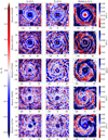 |
Fig. B.2 Continuation of Fig. B.1. |
| In the text | |
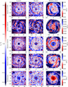 |
Fig. B.3 Continuation of Fig. B.2. |
| In the text | |
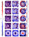 |
Fig. B.4 Continuation of Fig. B.3. |
| In the text | |
|
Fig. C.1 Distribution of particles in the correlation diagram δΣ vs. JR. The solid lines represent the linear fit of the particle density shown in the background map. The slope of the linear fit is provided in the inset text. |
| In the text | |
|
Fig. D.1 Density contrast maps for three distinct age intervals: stellar particles younger than 1 Gyr (left column), those aged between 1 and 2 Gyr (middle column), and those between 2 and 3 Gyr (right column) for a set of galaxies not shown in Fig. 8. Open circles indicate the spiral arm tracks inferred from Figs. B.1–B.4. Cross in the bottom-right corner indicates the scale of ±5 kpc. |
| In the text | |
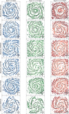 |
Fig. D.2 Continuation of Fig. D.1. |
| In the text | |
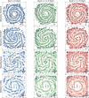 |
Fig. D.3 Continuation of Fig. D.2. |
| In the text | |
|
Fig. E.1 Visualisation of the border effect produced by the KDE technique on the δΣ map of the NEXUS simulations. Upper panel: scheme of the different configurations of the local (small squares) and global (large squares) scanning windows with respect to the boundary between a medium of uniform density Σ0 (grey area at negative Y) and the vacuum (white region at positive Y). Lower panel: values of δΣ for the mentioned configurations (red curve), assuming h = 0.5 kpc (vertical dotted lines) and H = 2.0 kpc (vertical dashed lines) bandwidths for the local and global kernels, respectively. |
| In the text | |
Current usage metrics show cumulative count of Article Views (full-text article views including HTML views, PDF and ePub downloads, according to the available data) and Abstracts Views on Vision4Press platform.
Data correspond to usage on the plateform after 2015. The current usage metrics is available 48-96 hours after online publication and is updated daily on week days.
Initial download of the metrics may take a while.