| Issue |
A&A
Volume 670, February 2023
|
|
|---|---|---|
| Article Number | L7 | |
| Number of page(s) | 11 | |
| Section | Letters to the Editor | |
| DOI | https://doi.org/10.1051/0004-6361/202245026 | |
| Published online | 30 January 2023 | |
Letter to the Editor
Spiral-like features in the disc revealed by Gaia DR3 radial actions⋆
1
Université Côte d’Azur, Observatoire de la Côte d’Azur, CNRS, Laboratoire Lagrange, France
e-mail: This email address is being protected from spambots. You need JavaScript enabled to view it.
2
Osservatorio Astrofisico di Torino, Istituto Nazionale di Astrofisica (INAF), 10025 Pino Torinese, Italy
3
Departament de Física Quàntica i Astrofísica (FQA), Universitat de Barcelona (UB), c. Martí i Franquès, 1, 08028 Barcelona, Spain
4
Institut de Ciències del Cosmos (ICCUB), Universitat de Barcelona (UB), c. Martí i Franquès, 1, 08028 Barcelona, Spain
5
Institut d’Estudis Espacials de Catalunya (IEEC), c. Gran Capità, 2-4, 08034 Barcelona, Spain
6
Lund Observatory, Department of Astronomy and Theoretical Physics, Lund University, Box 43 22100 Lund, Sweden
Received:
20
September
2022
Accepted:
4
December
2022
Abstract
Context. The so-called action variables are specific functions of the positions and velocities that remain constant along the stellar orbit. The astrometry provided by Gaia Early Data Release 3 (EDR3), combined with the velocities inferred from the Radial Velocity Spectrograph (RVS) spectra of Gaia DR3, allows for the estimation of these actions for the largest volume of stars to date.
Aims. We explore such actions with the aim of locating structures in the Galactic disc.
Methods. We computed the actions and the orbital parameters of the Gaia DR3 stars, assuming an axisymmetric model for the Milky Way. Using Gaia DR3 photometric data, we also selected a subset of giant stars with better astrometry as a control sample.
Results. We find that the maps of the percentiles of the radial action JR reveal arc-like segments. We found a high JR region centered at R ≈ 10.5 kpc of 1 kpc width, as well as three arc-shape regions dominated by circular orbits at inner radii. We also identified the spiral arms in the overdensities of the giant population.
Conclusions. For Galactic coordinates (X, Y, Z), we find good agreement with the literature in the innermost region for the Scutum-Sagittarius spiral arms. At larger radii, the low JR structure tracks the Local arm at negative X, while for the Perseus arm, the agreement is restricted to the X < 2 kpc region, with a displacement with respect to the literature at more negative longitudes. We detected a high JR area at a Galactocentric radii of ∼10.5 kpc, consistent with some estimations of the Outer Lindblad Resonance location. We conclude that the pattern in the dynamics of the old stars is consistent in several places with the spatial distribution of the spiral arms traced by young populations, with small potential contributions from the moving groups.
Key words: Galaxy: kinematics and dynamics / Galaxy: structure / Galaxy: disk
The orbital parameters and actions computed for this work are available at the CDS via anonymous ftp to cdsarc.cds.unistra.fr (130.79.128.5) or via https://cdsarc.cds.unistra.fr/viz-bin/cat/J/A+A/670/L7
© The Authors 2023
 Open Access article, published by EDP Sciences, under the terms of the Creative Commons Attribution License (https://creativecommons.org/licenses/by/4.0), which permits unrestricted use, distribution, and reproduction in any medium, provided the original work is properly cited.
This article is published in open access under the Subscribe-to-Open model. This email address is being protected from spambots. You need JavaScript enabled to view it. to support open access publication.
1. Introduction
The Gaia satellite (Gaia Collaboration 2016, 2018, 2022c; de Bruijne 2012) constitutes the most advanced astrometric mission to date. After its launch in 2013, it has been providing positions, parallaxes, proper motions, and line-of-sight (LoS) velocities for an increasing number of sources in subsequent data releases (Katz et al. 2004, 2019, 2022; Cropper et al. 2018). This exquisite astrometry has improved our understanding of Galactic structures that are already known, such as the spiral arms and the warp (Antoja et al. 2016; Poggio et al. 2018, 2021; Chrobáková et al. 2022; Gaia Collaboration 2022b), in addition to revealing a complex formation for the Milky Way and strong interactions with other galaxies (Belokurov et al. 2018; Myeong et al. 2018, 2019; Helmi et al. 2018; Koppelman et al. 2019; Helmi 2020). In this context, many asymmetries in different parameter spaces have been interpreted as a consequence of this scenario, including velocities (Antoja et al. 2017), distribution of proper motions (Palicio et al. 2020), ridges in projected velocities (Ramos et al. 2018; Fragkoudi et al. 2019; Khoperskov & Gerhard 2022; Gaia Collaboration 2022b,a; McMillan et al. 2022), distribution of actions (Hunt et al. 2019; Sellwood et al. 2019; Bland-Hawthorn et al. 2019; Trick et al. 2019, 2021; Trick 2022), and distribution of metallicity (Poggio et al. 2022). In this work, we report on structures in the Galactic plane revealed by the distribution of the radial action, JR, computed with the Gaia DR3 astrometry and LoS velocities (Gaia Collaboration 2022c).
This Letter is organised as follows. In Sect. 2, we explain the selection criteria applied to the Gaia data of our sample. In Sect. 3, we describe the model and the performance adopted for computing the orbital parameters and actions from the input data. Results are shown and discussed in Sects. 4 and 5, respectively. The conclusions can be found in Sect. 6. Finally, in Appendices A and B, we specify the data query performed on the Gaia archive1 and the detailed procedure for the estimation of the actions and orbital parameters, respectively. In Appendix C, we reproduce our analysis with a subsample of giants stars selected by photometry.
2. Gaia data and selection criteria
We made use of all the Gaia DR3 stars with full astrometric information available (parallaxes, positions, proper motions and line of sight velocities) and select those with non-null geometric distance estimation (Bailer-Jones et al. 2021). The corresponding ADQL query can be found in Appendix A. This sample totals 33 653 049 million sources – of these, we select the ones with good kinematic measurements by imposing a maximum LoS velocity error of 5 km s−1 and a relative error in proper motion lower than 15%. For the heliocentric distance, we imposed a maximum relative error of 20%. Since we have focussed our study on the disc, we excluded those stars whose maximum distance from the Galactic plane is larger than 500 pc (see Sect. 3). The resulting sample size is ∼12.4 million sources. We corrected the LoS velocities and proper motions, assuming (U⊙, V⊙, W⊙)=(9.5, 250.7, 8.56) km s−1 for the solar motion (GRAVITY Collaboration 2021; Reid & Brunthaler 2020) and R⊙ = 8.249 kpc for the Galactocentric distance of the Sun (GRAVITY Collaboration 2021).
In order to propagate the errors, we considered the correlations between the astrometric parameters. Motivated by the approach of Gaia Collaboration (2022b) and Kordopatis et al. (2022), we modelled the distribution of the errors of the geometric distances with a broken Gaussian distribution parameterised by the input confidence intervals (i.e. rlo and rhi in Bailer-Jones et al. 2021).
3. Orbital parameters and actions
We modeled the forces of the Milky Way with a rescaled version of the potential of McMillan (2017) such that the circular velocity at R⊙ = 8.249 kpc is V⊙ = 238.5 km s−1, consistent with our assumed Solar motion and the velocity of the Sun with respect to the local standard of rest taken from Schönrich et al. (2010). This potential is fully axisymmetric and models the contribution of the halo, bulge, and thin and thick stellar discs as well as the H I and H II gas discs. We estimate the orbital parameters (apocenter, rapo, pericenter, rperi, and maximum orbital distance to the galactic plane, Zmax) and the non-trivial actions, JR and JZ, by using own implementation of the Stäckel-Fudge approximation (Binney 2012; Sanders & Binney 2016; Mackereth & Bovy 2018). We refer to Appendix B for a detailed description of this procedure. Apart from these parameters, the vertical component of the angular momentum, Lz, and the total energy, E, are obtained as output. The actions, JR, JZ, and the angular momentum, Lz, presented in this work are expressed in units of L⊙ = R⊙V⊙.
4. Results
In this section, we explore the map of the distribution of the radial action JR in the Galactic Plane. Figure 1 shows the spatial distribution of the median JR, while each panel in Fig. 2 refers to other percentiles to illustrate the variation of the distribution of JR across the Galactic plane. Due to the variations in the observed trends as a function of the considered percentile, the colorbar is tuned to enhance the contrast between the high and low JR regions in each panel. We identify three main structures in the low JR regions for the first four percentiles shown in the figure (labelled as A, B, and C in Fig. 1), whereas for the 94th percentile, they are highly distorted. We observe an additional feature (labelled D) in the outer part of the disc (10 kpc ≲ R ≲ 11 kpc) characterised by high JR values. The innermost structure, labelled A, extends from R ≈ 6.0 kpc at (X, Y) ≈ (−2, −5.5) kpc to R ∼ 7 kpc at the solar azimuth (X = 0 kpc direction), while for X < 0 kpc it shows an almost constant radii of R ≈ 7 − 7.2 kpc. This results in a longitudinally asymmetric arc-shape structure of variable pitch angle.
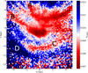 |
Fig. 1. Distribution of the median (equivalent to the P50 percentile) of JR on the Galactic Plane (|Zmax|< 0.5 kpc). The solid black circle denotes the solar position. Features labelled A to D are discussed in the text. |
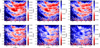 |
Fig. 2. Distribution of JR percentiles on the Galactic Plane (|Zmax|< 0.5 kpc). The x percentile is denoted by Px. The solid black circle denotes the solar position. |
Structure B also shows significant variations with longitude2: for X < 0 we observe a well-defined low JR area that extends from (X, Y) ≈ (−4, −6.5) kpc to (0, 8.5) kpc, embedding the solar neighbourhood. However, its prolongation at negative X is highly distorted, resulting in a wide area of low JR between structure A and the ℓ = −90° direction.
In contrast to the previous features, structure C is sharply defined at negative X, where it extends from (X, Y) ≈ (4, −9) kpc to (−2, −10) kpc, although it is possible to discern a tail of relatively low JR at X < −2 kpc. At positive X, this structure is connected with one of the extensions of the feature B, located in the large low JR area found between A and B (X > 0 kpc and −8 ≲ Y ≲ −7 kpc), and creating a gap of high JR with B. As can be seen in Fig. 2, this feature extends towards outer radii for percentiles larger than P83, and constitutes the only low JR structure at large percentile (P94).
The outermost feature (D) is a high JR region with an arc-shape of almost constant radii of 10.5 kpc and ∼1.0 kpc width. It remains almost unchanged for percentiles lower than P77 and becomes blurred for higher values. Apart from the main features, it is worthwhile mentioning the bifurcation in structure A at (X ≲ −2 kpc, Y ≈ −6 kpc) towards positive X, although it gets distorted in the maps for the large percentiles (P66 and above). Finally, we can discern a subtle arc-shape structure between A and B, with very low median radial action (P50 < 0.008) from (X, Y)≈(0, −7.7) to (2, −7.7).
In order to check whether the features described above are a consequence of the distribution of stars, we represent in Fig. 3 the density map of the selected sample. As it can be seen in the left panel, the density map cannot explain all the structures identified in Figs. 1 and 2. The density map peaks at the solar position and decreases with the heliocentric distance as fainter stars are excluded, showing no correspondence with the arc-shaped structures in the JR distribution.
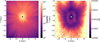 |
Fig. 3. Density map of the selected sample in the Cartesian plane (X, Y) on the left. Distribution of median errors in JR on the Galactic plane on the right. |
We verify the significance of the features in JR with the observational errors by evaluating the map of the median error of the radial action, δJR, estimated from 25 realisations of the input data (right panel in Fig. 3). Although it is possible to distinguish some selection effects in an annular region centred at the Sun, the structure associated with them does not correspond to that reported in Figs. 1 and 2. Furthermore, in the vast majority of the plane, the errors of JR are at least 3.5 times smaller than the median JR, supporting the robustness of the features found in the percentile distributions.
5. Discussion
In this section, we discuss three possible scenarios to explain the observed features in JR.
5.1. Spiral arms
The spatial distribution and shape of the structures reported above suggest a connection with the spiral arms. To explore this hypothesis, we compare these structures with the fit of the spiral arms inferred from the kinematics of one hundred masers (Reid et al. 2014) from the distribution of Cepheids (Lemasle et al. 2022) and from the distribution of Gaia EDR3 upper main sequence stars (UMS stars, Poggio et al. 2021), which considers the same astrometric measurements (but for a different sample) as this work. We complement these references with the overdensity map of our subsample of giant stars (see Appendix C). Following the procedure described in Poggio et al. (2021), we compute the local (average) density using an Epanechnikov kernel (Epanechnikov 1969) of bandwidth 0.3 kpc (2.0 kpc). This kernel assumes that the contribution of a star to the density at a reference point is weighted by a term ∝max{1 − x2/h2, 0}, where h is the bandwidth and x is the separation between the star and the reference point. For sake of visualisation, the references of spiral arms described above are shown in individual panels in Fig. 4.
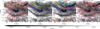 |
Fig. 4. Comparison of the maps of P50(JR) with the spiral arms reported in literature. First panel: contour lines enclose the overdensities found in the subsample of giants. Second panel: solid lines represent the Scutum (cyan), Sagittarius (yellow), Local (blue), and Perseus (black) spiral arms of Reid et al. (2014), while the dotted lines correspond to their extrapolation in azimuth. Third panel: Solid lines represent the segments of spiral arms of Lemasle et al. (2022), in which their same naming convention is used, while the colorcode results from a visual comparison with these of Reid et al. (2014). The additional structures are indicated by red and pink lines for description convenience. Fourth panel: contour lines illustrate the overdensities reported by Poggio et al. (2021). Background image: reproduction of Fig. 1 using a grey color-scale to increase the contrast between the coloured lines and the background map. The solid white circle denotes the solar position. |
The first panel in Fig. 4 illustrates the overdensities in the distribution of our sample of giants. We find a correspondence between the overdensities in this sample and these reported by Poggio et al. (2021) for the younger UMS population (fourth panel); although some discrepancies are observed at (X, Y)≈(−1, −9) kpc and (−2,−6.5) kpc. The presence of the spiral arms traced by an old population has been recently proposed by Lin et al. (2022), who identified the Local Arm in a sample of 87 000 Gaia EDR3-2MASS (Gaia Collaboration 2021; Skrutskie et al. 2006), Red Clump stars (RC) and could be related to the metallicity asymmetry in Sample B and C in Poggio et al. (2022, see their Fig. 1).
In general terms, we find a good agreement between the low JR areas and the spiral arms, especially in the innermost regions, where the distribution of giant stars (first panel) reveals an overdensity consistent with Structure A. Furthermore, the bifurcation observed in A can be explained by segments 16 and 22 of Lemasle et al. (2022), likely to be part of Sagittarius and Scutum, respectively. On the contrary, we find a shift of ∼0.5 kpc between structure A and the location of segment 9, where the extrapolation of Reid et al. (2014) fits the lowest JR region of A (dotted lines) perfectly. Compared to Poggio et al. (2021), we can identify most of Structure A in the innermost overdensity of UMS stars, although no bifurcation is observed at X ≈ −2 kpc. The extension of this overdensity, however, is compatible with the area of low JR that connects the structures A and B in Fig. 1.
As mentioned in Sect. 4, we find a subtle arc-shape structure between A and B close to the solar neighbourhood. This feature has no counterpart in the spiral arms of Reid et al. (2014) and Poggio et al. (2021) or in our distribution of giant stars, but it is located at the same position as the segment 18 (pink line) of Lemasle et al. (2022), being a potential continuation of the Sagittarius arm. As the percentile increases (Fig. 2), this small area of low JR becomes more evident (a gap with A emerges) and consistent with the segment 18 and its extension towards positive X.
The part of structure B located at negative X is compatible with the fit of the Local spiral arm of Reid et al. (2014), the segment 23 of Lemasle et al. (2022) and the overdense regions found in the UMS and giant population. On the contrary, at positive X only the Local arm of Reid et al. (2014) might provide a good explanation for structure B, but only if a shift of ∼0.5 kpc is considered. It is worthwhile mentioning the significant differences among the references for that part of the Local arm: assuming the segment labelled 17 is part of the Local arm, it implies a pitch angle of opposite sign compared to that in Poggio et al. (2021); whereas according to Reid et al. (2014), the Local arm is more tangential. This variety of observations suggests a complex definition of the extension and limits of the Local spiral arm despite its proximity to the Sun.
One major discrepancy is found in the solar neighbourhood: according to our maps, the Sun is embedded in the intersection of the Local and the Sagittarius spiral arm, while the predictions of all three spiral arms maps report a solar location in the inner boundary of the Local Arm.
The JR maps suggest a connection between the Perseus and the Local Arm (Structures C and B, respectively). However, the spatial geometry of the spiral arms from UMS stars (Poggio et al. 2021), Red Clump stars (Lin et al. 2022), and the giant sample does not coincide with the observed features in JR in this region.
The comparison of structure C reveals a good agreement with the Perseus spiral arm of Reid et al. (2014) for X ≲ 0 kpc and the segment 12 of Lemasle et al. (2022) within |X|≲1 kpc. However, at positive X, structure C exhibits a different pitch angle, as compared to both Reid et al. (2014) and Lemasle et al. (2022).
It is worth mentioning that the spiral structure of the Milky Way might be different depending on the considered stellar population. Here, the contrast in JR is observed mainly in the giant old population (see Appendix C for the specific analysis of the giant stars), even though the stars in the spiral arms tend to be young and, through the age–velocity dispersion relation, exhibit lower values of JR. For instance, the referred spiral arms have been traced by selecting masers, Cepheids and UMS stars, namely, the young population. Thus, the dynamics of the old stars seem to be in agreement with the spatial distribution of the young population in some regions, but present some discrepancies in others. Such discrepancies can be either due to the fact that the geometry of the spiral arms might be different for different stellar populations or that the dynamical nature of the spiral arms somehow leads to the observed features.
5.2. Moving groups
We also explored the possible origin of the reported structures in the moving groups. As Ramos et al. (2018) have shown, it is possible to identify the moving groups as stripes in the azimuthal velocity, Vϕ vs. R, diagram. Figure 5 represents the distribution of the median JR in the (R,Vϕ) plane, including some of the moving groups reported by Ramos et al. (2018) as reference (yellow dashed lines). For sake of visualisation, we focus on the range 220 < Vϕ < 250 km s−1 and use a logarithmic colorscale for median(JR) to enhance the features. As expected, the values of JR tend to increase as Vϕ differs from the rotation curve. As Fig. 5 shows, the Dehnen98-6, Hyades and Sirius moving groups are predominantly located in areas of relatively high JR in the (R,Vϕ) plane, in contrast to the low JR values that characterise the features described in Sect. 4. On the contrary, Coma Berenices lies close to a transition from low to high JR. The Hercules and most of the Horn-Dehnen98 moving groups lie in the region of high JR (blue saturated region) and we do not see any clear correspondence for the Arch1-Hat moving group at this point. In any case, these groups could be related to the structures of JR in the R − Vϕ projection that extend to higher JR (not seen in our figures due to the colour range).
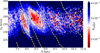 |
Fig. 5. Azimuthal velocity Vϕ vs. R diagram colorcoded with the median JR. The colorbar has been intentionally set in logarithmic scale to cover a wide range of values in JR. The moving groups (dashed yellow lines) are displayed from the bottom left to the upper right corner as follows: Hercules, Dehnen98-6, Horn-Dehnen98, Hyades, Coma Berenices, Sirius, and Arch1-Hat. Black ellipses enclose the two selected areas (see the text), while the Sun is denoted by the solid black circle. |
Apart from the ridges, we can identify two interesting areas of low JR: one located between the Dehnen98-6 and the Hyades moving groups (as a prolongation of Horn-Dehnen98 at inner radii) and another more extended low JR area close to Coma Berenices. In order to evaluate the contribution of this potential members of moving groups, we exclude the stars within these regions (black dashed ellipses in Fig. 5). We have verified the exclusion of the stars close to Coma Berenices raises the median values of JR at ∼(2, −8) kpc, improving the separation between the A and B structures at positive X. The exclusion of the other selection, however, leads to an annular distortion at R ∼ 7.7 kpc that increases the gap between the A and B structures, especially at negative X. This distortion, however, is more likely to be an artefact caused by the exclusion of a significant number of sources within 7.6 ≲ R ≲ 8.0 kpc, rather than a true contribution of the Horn-Dehnen moving group.
Based on our tests, the features observed in the Vϕ vs. R plane are not as clear as those found in the maps of JR, although an apparent relation between the high JR values and the position of some ridges can be inferred. A deeper analysis of this relation is needed to evaluate the contribution of the moving groups to the features in JR(X, Y) and (potentially) its connection with the spiral arms. Such an analysis is beyond the scope of this Letter and will be explored in a future work.
5.3. Galactic bar
Apart from the spiral arms, the location and shape of the high JR region at R ∼ 10.5 kpc is consistent with some values reported for the Outer Lindblad Resonance (OLR; Liu et al. 2012; Portail et al. 2017; Pérez-Villegas et al. 2017). In order to evaluate this possible connection, we must verify whether the OLR corresponds to a region of increasing radial action. Under the epicyclic approximation (see Binney & Tremaine 2008), the Galactocentric distance R(t) of a star trapped by a resonance varies with time as:
 (1)
(1)
where the factor of 2 in the cosine comes from the assumption of a dipolar disturbance of the potential (m = 2), Rg is the guiding radius, Ω is the circular frequency at Rg, Ωp is the pattern speed, and C2 is a constant that depends on the bar potential Φb(R, ϕ, t) as:
 (2)
(2)
with κ the epicyclic frequency at R = Rg. Differentiating Eq. (1) with respect to the time and substituting in the integral for JR (see Eq. (B.11)) we have:
 (3)
(3)
where the upper and lower limits correspond to the cases in which cos(ΔΩt) = −1 (apocenter) and +1 (pericenter), respectively. Thus, Eq. (3) diverges in the Outer Lindblad Resonance (κ + 2ΔΩ = 0). Although Eq. (1) assumes a small deviation in azimuth with respect to the circular orbit defined by the guiding radius, which is not true in the resonance regime, it is enough to demonstrate the radial action increases towards the resonances (Chiba & Schönrich 2021). A more detailed analysis, such as that described for the corotation in Sect. 3.3b of Binney & Tremaine (2008), would predict a large but finite action. However, the calculus of this more general case is not straightforward (Goldreich & Tremaine 1981).
According to Sellwood & Binney (2002) and Sellwood (2010), it is not only the OLR, but also the inner Lindblad resonance (ILR), that should be characterised by an increment in JR due to the outward flow of angular momentum (Lynden-Bell & Kalnajs 1972). Assuming a pattern speed for the bar between 34 and 47 km s−1 kpc−1 (Bland-Hawthorn & Gerhard 2016, and references therein), the ILR is expected to be located out of our region of study.
6. Conclusions
The statistics of the radial actions reveal arc-shape structures in the Galactic disc. These structures are characterised by a predominance of more circular orbits that contrasts to the high radial action feature found at R ∼ 10.5 kpc. The analysis of the errors in JR confirms the reported structures are not spurious but robust from the statistical point of view. Furthermore, they cannot be explained by the selection effects inherent in Gaia.
The characteristic arc shape of the structures in JR motivates the comparison with the Milky Way spiral arms, whose fit parameters have been reported in previous studies. We find that in the innermost region, structure A clearly defines the Sagittarius arm, with its upper boundary is delimited by the Scutum arm. At larger Galactocentric radii, structure B tracks the Local Arm at negative X, while no clear correspondence with literature is found at X > 0, where the variety of models suggests a complex definition for this arm. On the contrary, for the Perseus Arm we observe a good concordance with the spatial distribution of young stellar population for X ∈ ( − 2, 0) kpc, while at positive X, the orientation of the JR feature has a different pitch angle compared to all the considered models. Our results suggest that the Perseus Arm in the JR map is connected to the Local Arm at ∼3.6 kpc from the Sun, in the direction of ℓ ≈ −100°. This would result in a mismatch with some geometries of the spiral arms from young stellar populations, which will be studied in the future. We observe a correspondence between the segment 18 in Lemasle et al. (2022) and a region of very low JR between structures A and B that has not clear spiral arm assignation.
We also explored the moving groups as a possible explanation for the features. The JR arc-shape structures in the (X, Y) plane are likely to be related to the structures in JR in the R − Vϕ plane but mapped onto different projections of phase space, in particular, showing also their complex dependency with position (e.g., azimuth) in the (X, Y) case. We observe some features in the Vϕ vs. R plane that might be anti-correlated with some known moving groups. However, this connection between the moving groups and the JR features in the Galactic plane, if present, is not obvious and should be explored in future studies.
We identify an area of high radial action centered at ∼10.5 kpc, where the outer Lindblad resonance (OLR) caused by the bar is expected. Apart from the features in the maps of the radial action, we find the distribution of the giant stars in the disc is consistent with the spiral arms traced by younger populations, in particular: the upper main sequence stars.
The analysis presented in this work indicate that multiple agents might be causing the structures found in the distribution of JR. Although the spiral arms account for most of the features reported in this work, there are still many discrepancies that must be addressed. In this context, further studies with numerical simulations and analytical models are required to explain these differences and shed light on the Galactic dynamics.
We denote the Galactic longitude and latitude with (ℓ, b), respectively, where ℓ increases counter-clockwise from the Sun-Galactic centre direction.
Defined as σ = 1.48 × median(|x − median(x)|) for consistency with the standard deviation.
Acknowledgments
The authors acknowledge J. Bland-Hawthorn for his constructive contribution to this work as referee. We thank P. de Laverny for his useful comments. P. A. Palicio acknowledges the financial support from the Centre national d’études spatiales (CNES). E. Spitoni and A. Recio-Blanco received funding from the European Union’s Horizon 2020 research and innovation program under SPACE-H2020 grant agreement number 101004214 (EXPLORE project). This project has received funding from the European Union’s Horizon 2020 research and innovation programme under the Marie Sklodowska-Curie grant agreement N. 101063193. TA acknowledges the grant RYC2018-025968-I funded by MCIN/AEI/10.13039/501100011033 and by “ESF Investing in your future”. This work was (partially) funded by the Spanish MICIN/AEI/10.13039/501100011033 and by “ERDF A way of making Europe” by the “European Union” through grant RTI2018-095076-B-C21, and the Institute of Cosmos Sciences University of Barcelona (ICCUB, Unidad de Excelencia ‘María de Maeztu’) through grant CEX2019-000918-M. PJM acknowledges project grants from the Swedish Research Council (Vetenskaprådet, Reg: 2017- 03721; 2021-04153). This work has made use of data from the European Space Agency (ESA) mission Gaia (https://www.cosmos.esa.int/gaia), processed by the Gaia Data Processing and Analysis Consortium (DPAC, https://www.cosmos.esa.int/web/gaia/dpac/consortium). Funding for the DPAC has been provided by national institutions, in particular the institutions participating in the Gaia Multilateral Agreement. Although GALPY is not explicitly used in this work, P. A. Palicio uses its source code as reference and recognises the credit for the work of Bovy (2015).
References
- Antoja, T., Roca-Fàbrega, S., de Bruijne, J., & Prusti, T. 2016, A&A, 589, A13 [NASA ADS] [CrossRef] [EDP Sciences] [Google Scholar]
- Antoja, T., de Bruijne, J., Figueras, F., et al. 2017, A&A, 602, L13 [EDP Sciences] [Google Scholar]
- Bailer-Jones, C. A. L., Rybizki, J., Fouesneau, M., Demleitner, M., & Andrae, R. 2021, AJ, 161, 147 [Google Scholar]
- Belokurov, V., Erkal, D., Evans, N. W., Koposov, S. E., & Deason, A. J. 2018, MNRAS, 478, 611 [Google Scholar]
- Binney, J. 2012, MNRAS, 426, 1324 [Google Scholar]
- Binney, J., & Tremaine, S. 2008, Galactic Dynamics, 2nd edn. (Princeton: Princeton University Press) [Google Scholar]
- Bland-Hawthorn, J., & Gerhard, O. 2016, ARA&A, 54, 529 [Google Scholar]
- Bland-Hawthorn, J., Sharma, S., Tepper-Garcia, T., et al. 2019, MNRAS, 486, 1167 [NASA ADS] [CrossRef] [Google Scholar]
- Bovy, J. 2015, ApJS, 216, 29 [NASA ADS] [CrossRef] [Google Scholar]
- Chiba, R., & Schönrich, R. 2021, MNRAS, 505, 2412 [NASA ADS] [CrossRef] [Google Scholar]
- Chrobáková, Ž., Nagy, R., & López-Corredoira, M. 2022, A&A, 664, A58 [NASA ADS] [CrossRef] [EDP Sciences] [Google Scholar]
- Cropper, M., Katz, D., Sartoretti, P., et al. 2018, A&A, 616, A5 [NASA ADS] [CrossRef] [EDP Sciences] [Google Scholar]
- de Zeeuw, T. 1985, MNRAS, 216, 273 [NASA ADS] [CrossRef] [Google Scholar]
- de Bruijne, J. H. J. 2012, Ap&SS, 341, 31 [NASA ADS] [CrossRef] [Google Scholar]
- Epanechnikov, V. A. 1969, Theory Probab. Appl., 14, 153 [Google Scholar]
- Fragkoudi, F., Katz, D., Trick, W., et al. 2019, MNRAS, 488, 3324 [NASA ADS] [Google Scholar]
- Gaia Collaboration (Prusti, T., et al.) 2016, A&A, 595, A1 [NASA ADS] [CrossRef] [EDP Sciences] [Google Scholar]
- Gaia Collaboration (Brown, A. G. A., et al.) 2018, A&A, 616, A1 [NASA ADS] [CrossRef] [EDP Sciences] [Google Scholar]
- Gaia Collaboration (Brown, A. G. A., et al.) 2021, A&A, 649, A1 [NASA ADS] [CrossRef] [EDP Sciences] [Google Scholar]
- Gaia Collaboration (Drimmel, R., et al.) 2022a, https://doi.org/10.1051/0004-6361/202243797 [Google Scholar]
- Gaia Collaboration (Recio-Blanco, A., et al.) 2022b, https://doi.org/10.1051/0004-6361/202243511 [Google Scholar]
- Gaia Collaboration (Vallenari, A., et al.) 2022c, A&A, 161, 147 [Google Scholar]
- Goldreich, P., & Tremaine, S. 1981, ApJ, 243, 1062 [NASA ADS] [CrossRef] [Google Scholar]
- GRAVITY Collaboration (Abuter, R., et al.) 2021, A&A, 654, A22 [NASA ADS] [CrossRef] [EDP Sciences] [Google Scholar]
- Helmi, A. 2020, ARA&A, 58, 205 [Google Scholar]
- Helmi, A., Babusiaux, C., Koppelman, H. H., et al. 2018, Nature, 563, 85 [Google Scholar]
- Hunt, J. A. S., Bub, M. W., Bovy, J., et al. 2019, MNRAS, 490, 1026 [NASA ADS] [CrossRef] [Google Scholar]
- Katz, D., Munari, U., Cropper, M., et al. 2004, MNRAS, 354, 1223 [NASA ADS] [CrossRef] [Google Scholar]
- Katz, D., Sartoretti, P., Cropper, M., et al. 2019, A&A, 622, A205 [NASA ADS] [CrossRef] [EDP Sciences] [Google Scholar]
- Katz, D., Sartoretti, P., Guerrier, A., et al. 2022, https://doi.org/10.1051/0004-6361/202244220 [Google Scholar]
- Khoperskov, S., & Gerhard, O. 2022, A&A, 663, A38 [NASA ADS] [CrossRef] [EDP Sciences] [Google Scholar]
- Koppelman, H. H., Helmi, A., Massari, D., Price-Whelan, A. M., & Starkenburg, T. K. 2019, A&A, 631, L9 [NASA ADS] [CrossRef] [EDP Sciences] [Google Scholar]
- Kordopatis, G., Schultheis, M., McMillan, P.J., et al. 2022, A&A, submitted [arXiv:2206.07937] [Google Scholar]
- Lemasle, B., Lala, H. N., Kovtyukh, V., et al. 2022, A&A, 668, A40 [NASA ADS] [CrossRef] [EDP Sciences] [Google Scholar]
- Lin, Z., Xu, Y., Hou, L., et al. 2022, ApJ, 931, 72 [NASA ADS] [CrossRef] [Google Scholar]
- Liu, C., Xue, X., Fang, M., et al. 2012, ApJ, 753, L24 [NASA ADS] [CrossRef] [Google Scholar]
- Lynden-Bell, D., & Kalnajs, A. J. 1972, MNRAS, 157, 1 [Google Scholar]
- Mackereth, J. T., & Bovy, J. 2018, PASP, 130, 114501 [Google Scholar]
- McMillan, P. J. 2017, MNRAS, 465, 76 [NASA ADS] [CrossRef] [Google Scholar]
- McMillan, P. J., Petersson, J., Tepper-Garcia, T., et al. 2022, MNRAS, 516, 4988 [NASA ADS] [CrossRef] [Google Scholar]
- Myeong, G. C., Evans, N. W., Belokurov, V., Amorisco, N. C., & Koposov, S. E. 2018, MNRAS, 475, 1537 [NASA ADS] [CrossRef] [Google Scholar]
- Myeong, G. C., Vasiliev, E., Iorio, G., Evans, N. W., & Belokurov, V. 2019, MNRAS, 488, 1235 [Google Scholar]
- Palicio, P. A., Martinez-Valpuesta, I., Allende Prieto, C., & Dalla Vecchia, C. 2020, A&A, 634, A90 [NASA ADS] [CrossRef] [EDP Sciences] [Google Scholar]
- Pérez-Villegas, A., Portail, M., Wegg, C., & Gerhard, O. 2017, ApJ, 840, L2 [Google Scholar]
- Poggio, E., Drimmel, R., Lattanzi, M. G., et al. 2018, MNRAS, 481, L21 [Google Scholar]
- Poggio, E., Drimmel, R., Cantat-Gaudin, T., et al. 2021, A&A, 651, A104 [NASA ADS] [CrossRef] [EDP Sciences] [Google Scholar]
- Poggio, E., Recio-Blanco, A., Palicio, P. A., et al. 2022, A&A, 666, L4 [NASA ADS] [CrossRef] [EDP Sciences] [Google Scholar]
- Portail, M., Gerhard, O., Wegg, C., & Ness, M. 2017, MNRAS, 465, 1621 [NASA ADS] [CrossRef] [Google Scholar]
- Ramos, P., Antoja, T., & Figueras, F. 2018, A&A, 619, A72 [NASA ADS] [CrossRef] [EDP Sciences] [Google Scholar]
- Reid, M. J., & Brunthaler, A. 2020, ApJ, 892, 39 [Google Scholar]
- Reid, M. J., Menten, K. M., Brunthaler, A., et al. 2014, ApJ, 783, 130 [Google Scholar]
- Ripepi, V., Clementini, G., Molinaro, R., et al. 2022, https://doi.org/10.1051/0004-6361/202243990 [Google Scholar]
- Sanders, J. L., & Binney, J. 2016, MNRAS, 457, 2107 [Google Scholar]
- Schönrich, R., Binney, J., & Dehnen, W. 2010, MNRAS, 403, 1829 [NASA ADS] [CrossRef] [Google Scholar]
- Sellwood, J. A. 2010, MNRAS, 409, 145 [NASA ADS] [CrossRef] [Google Scholar]
- Sellwood, J. A., & Binney, J. J. 2002, MNRAS, 336, 785 [Google Scholar]
- Sellwood, J. A., Trick, W. H., Carlberg, R. G., Coronado, J., & Rix, H.-W. 2019, MNRAS, 484, 3154 [NASA ADS] [CrossRef] [Google Scholar]
- Skrutskie, M. F., Cutri, R. M., Stiening, R., et al. 2006, AJ, 131, 1163 [NASA ADS] [CrossRef] [Google Scholar]
- Trick, W. H. 2022, MNRAS, 509, 844 [Google Scholar]
- Trick, W. H., Coronado, J., & Rix, H.-W. 2019, MNRAS, 484, 3291 [NASA ADS] [CrossRef] [Google Scholar]
- Trick, W. H., Fragkoudi, F., Hunt, J. A. S., Mackereth, J. T., & White, S. D. M. 2021, MNRAS, 500, 2645 [Google Scholar]
Appendix A: ADQL query
SELECT source_id, ra, dec, pmra, pmdec,
 radial_velocity, parallax, ruwe, ra_error,
 dec_error, pmra_error, pmdec_error,
 radial_velocity_error, parallax_error,
 ra_dec_corr, ra_pmra_corr, ra_pmdec_corr,
 dec_pmra_corr, dec_pmdec_corr, pmra_pmdec_corr,
 grvs_mag,r_med_geo, r_lo_geo, r_hi_geo
FROM user_dr3int6.gaia_source INNER JOIN
 external.gaiaedr3_distance USING(source_id)
WHERE (radial_velocity is not NULL) and (pmra is not
 NULL) and (pmdec is not NULL)
Listing 1. ADQL query for the Gaia DR3 considered in this work.
Appendix B: Stäckel-Fudge approximation
Within this approach, the orbital parameters can be computed assuming the considered Galactic potential Φ(R, z) satisfies some properties of the so-called Stäckel potentials. Given an axisymmetric oblate distribution of mass, its potential Φ(R, z) is said to be a Stäckel potential if there are two single-variable functions U(u) and V(v) such that:
 (B.1)
(B.1)
where (u, v) are the ellipsoidal coordinates (de Zeeuw 1985) related to (R, z) through the transformation:
 (B.2)
(B.2)
with Δ as the focal length of the elliptical (hyperbolic) curves of constant u (v). Since the Galactic potential is known to be oblate, we do not describe the prolate case (for the prolate case see de Zeeuw 1985). By differentiating both sides of Eq. B.2 with respect to time, the transformation of the momentum between (R, z) and the (u, v) coordinate systems is as follows:
 (B.3)
(B.3)
where pi is the momentum associated with the coordinate i ∈ {R, z, u, v}. The Hamiltonian constructed with the momenta of Eq.B.3 and the potential ΦS(u, v) results in a expression that can be separated into two single variable terms:
 (B.4)
(B.4)
in which E is the total energy of the system (since the Hamiltonian does not depend explicitly on time), Lz is the vertical component of the angular momentum, and I3 is the third integral of motion.
For a reference point with coordinates (u, v)=(u0, π/2), the expression for u in Eq. B.4 is:
 (B.5)
(B.5)
 (B.6)
(B.6)
where the choice for u0 is discussed later. Subtracting Eq. B.4 from B.5 and solving for pu we find:
 (B.7)
(B.7)
where the term δU ≡ U(u)−U(u0) can be approximated using the definition of the Stäckel potential (Eq. B.1) as:
 (B.8)
(B.8)
Similarly, we can define δV = V(v)−V(π/2) such that:
 (B.9)
(B.9)
then pv can be written as
 (B.10)
Expressions B.7 and B.10 for pu and pv, respectively, can be substituted in the integrals for the definition of the actions (see Eq. 6 in Binney 2012):
 (B.11)
 (B.12)
Both the limits and the integrals of Eq. B.11 have to be computed numerically. The limits of integration correspond to the roots of Eq. B.7 and B.10 (therefore, the actions are always real). In our case, we computed these roots using the bisection method, while the numerical integration is performed by Gaussian Quadrature with ten nodes. We approximated the radial and vertical actions as JR ≈ Ju and Jz ≈ Jv, respectively, since the R (z) coordinate varies more with u (v), as Fig B.1 illustrates. The choice of u0 is rather arbitrary (see Section 2 in Binney (2012) for the discussion), so we use the coordinate u given by the input value (R, z) of the star.
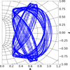 |
Fig. B.1. Example of an orbit in the (R, Z) plane (blue curve) with the lines of constant u (dot-dashed ellipses) and v (dashed hyperbolas) in the background. The units of the axis are arbitrary. |
In order to account for the error propagation, we performed 25 random realisations of the input data and compute the median values and the 16th and 84th percentiles of the output.
Appendix C: Results with the subsample of giants
Using a photometric selection of stars, we demonstrate that the dynamical pattern reported here is mainly supported by the old giant population, although the stars in spiral arms tend to be younger than average and, therefore, they have lower values of JR according to the age-velocity dispersion relation. We reproduce the percentiles of JR (shown in Fig. 2) by applying the following photometric criteria:
 (C.1)
(C.1)
which assumes no extinction as a first approximation to restrict the sample to the giants (hereafter, we refer to this subset as ’giant subsample’). The expression in Eq. C.1 visually separates the red giant branch (RGB) from the main sequence stars in the Hertzsprung–Russell (HR) diagram, using the red clump as reference for the boundary (Fig. C.1). By selecting giants, we are able to retain stars intrinsically brighter and reduce the effect of the selection function as well as the contribution from the faint dwarf stars that dominate the sample in the Solar neighbourhood (Gaia Collaboration 2022b).
Figure C.2 illustrates the distribution of the percentiles of JR for the ’giant’ subsample. In general, the features found in the whole sample are observed in the giant subsample, with the exception of the high JR region between the Local and Perseus (B-C) arm which is more distorted. Similarly, the high radial action region near the Sun disappears. In contrast to Fig. 3, for the giant subsample, the highest density area corresponds to the innermost low JR region, although no evidence of the other structures are observed.
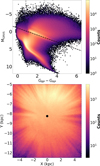 |
Fig. C.1. Distribution of stars in the Hertzsprung–Russell diagram for the Galactic disc sample (|Zmax|< 0.5 kpc) shown in the upper panel. The dashed black line represents the boundary condition considered to separate Main Sequence and RGB stars (Eq. C.1) neglecting extinction. Density map of the giant sample in the (X, Y) plane in the bottom panel. The solar position is denoted by a solid black circle. |
 |
Fig. C.2. Distribution of JR percentiles for the giant subsample. Details are the same as those in Fig. 2. Upper-left panel corresponds to the median (equivalent to Fig. 1), while two additional percentiles are shown in the central and right upper panels. |
We performed an additional test to address the age of the tracers of the arc-shaped structures. We compared the kinematics of our giant sample with that of the Cepheids in Gaia DR3 (Ripepi et al. 2022) to get a proxy of the relative age of both populations. In Fig. C.3, we show the distributions of azimuthal (Vϕ) and vertical velocities (VZ) for the Cepheid and giant subsamples. As we can see, the distribution of Vϕ for the Cepheids is more peaked than that of the giants, as expected for cooler (and younger) populations, with a median absolute deviation3 of σC = 36.05 km/s (σG = 20.41 km/s) for the Cepheid (giant) samples. Similarly, the distribution of VZ observed for the giant subsample is consistent with a hotter and older population compared to the Cepheids, with σG = 22.56 km/s and σC = 8.56 km/s, respectively. Therefore, the distributions presented in Fig. C.3 indicate that the giant subsample is dominated by stars typically older than the Cepheids.
It is interesting to note that our sample is typically old, whereas the spiral arms feature is most often seen in young stars (classical Cepheids, masers, and UMS stars). When comparing the features in JR to the spiral arms, we should therefore bear in mind that intrinsic differences might be present because they are two different populations.
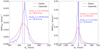 |
Fig. C.3. Probability distribution function of the azimuthal (left panel) and vertical (right panel) velocities for the subsample of giant stars (red bars) and Cepheids (blue bars). The median values (P50) and median absolute deviations (σ) for both samples are indicated in the inset. Vertical dashed lines denote median values. |
All Figures
|
Fig. 1. Distribution of the median (equivalent to the P50 percentile) of JR on the Galactic Plane (|Zmax|< 0.5 kpc). The solid black circle denotes the solar position. Features labelled A to D are discussed in the text. |
| In the text | |
|
Fig. 2. Distribution of JR percentiles on the Galactic Plane (|Zmax|< 0.5 kpc). The x percentile is denoted by Px. The solid black circle denotes the solar position. |
| In the text | |
|
Fig. 3. Density map of the selected sample in the Cartesian plane (X, Y) on the left. Distribution of median errors in JR on the Galactic plane on the right. |
| In the text | |
|
Fig. 4. Comparison of the maps of P50(JR) with the spiral arms reported in literature. First panel: contour lines enclose the overdensities found in the subsample of giants. Second panel: solid lines represent the Scutum (cyan), Sagittarius (yellow), Local (blue), and Perseus (black) spiral arms of Reid et al. (2014), while the dotted lines correspond to their extrapolation in azimuth. Third panel: Solid lines represent the segments of spiral arms of Lemasle et al. (2022), in which their same naming convention is used, while the colorcode results from a visual comparison with these of Reid et al. (2014). The additional structures are indicated by red and pink lines for description convenience. Fourth panel: contour lines illustrate the overdensities reported by Poggio et al. (2021). Background image: reproduction of Fig. 1 using a grey color-scale to increase the contrast between the coloured lines and the background map. The solid white circle denotes the solar position. |
| In the text | |
|
Fig. 5. Azimuthal velocity Vϕ vs. R diagram colorcoded with the median JR. The colorbar has been intentionally set in logarithmic scale to cover a wide range of values in JR. The moving groups (dashed yellow lines) are displayed from the bottom left to the upper right corner as follows: Hercules, Dehnen98-6, Horn-Dehnen98, Hyades, Coma Berenices, Sirius, and Arch1-Hat. Black ellipses enclose the two selected areas (see the text), while the Sun is denoted by the solid black circle. |
| In the text | |
|
Fig. B.1. Example of an orbit in the (R, Z) plane (blue curve) with the lines of constant u (dot-dashed ellipses) and v (dashed hyperbolas) in the background. The units of the axis are arbitrary. |
| In the text | |
|
Fig. C.1. Distribution of stars in the Hertzsprung–Russell diagram for the Galactic disc sample (|Zmax|< 0.5 kpc) shown in the upper panel. The dashed black line represents the boundary condition considered to separate Main Sequence and RGB stars (Eq. C.1) neglecting extinction. Density map of the giant sample in the (X, Y) plane in the bottom panel. The solar position is denoted by a solid black circle. |
| In the text | |
|
Fig. C.2. Distribution of JR percentiles for the giant subsample. Details are the same as those in Fig. 2. Upper-left panel corresponds to the median (equivalent to Fig. 1), while two additional percentiles are shown in the central and right upper panels. |
| In the text | |
|
Fig. C.3. Probability distribution function of the azimuthal (left panel) and vertical (right panel) velocities for the subsample of giant stars (red bars) and Cepheids (blue bars). The median values (P50) and median absolute deviations (σ) for both samples are indicated in the inset. Vertical dashed lines denote median values. |
| In the text | |
Current usage metrics show cumulative count of Article Views (full-text article views including HTML views, PDF and ePub downloads, according to the available data) and Abstracts Views on Vision4Press platform.
Data correspond to usage on the plateform after 2015. The current usage metrics is available 48-96 hours after online publication and is updated daily on week days.
Initial download of the metrics may take a while.