| Issue |
A&A
Volume 695, March 2025
|
|
|---|---|---|
| Article Number | A278 | |
| Number of page(s) | 18 | |
| Section | Interstellar and circumstellar matter | |
| DOI | https://doi.org/10.1051/0004-6361/202453386 | |
| Published online | 27 March 2025 | |
FAUST
XXIII. SiO outflow in the protobinary system L483
1
National Astronomical Observatory of Japan,
2-12 Hoshigaoka, Mizusawa, Oshu,
Iwate
023-0861,
Japan
2
SOKENDAI (The Graduate University for Advanced Studies),
2-21-1 Osawa, Mitaka,
Tokyo
181-8588,
Japan
3
Université de Bordeaux – CNRS Laboratoire d’Astrophysique de Bordeaux,
33600
Pessac,
France
4
Center for Gravitational Physics, Yukawa Institute for Theoretical Physics, Kyoto University,
Oiwake-cho, Kitashirakawa, Sakyo-ku, Kyoto-shi,
Kyoto-fu
606-8502,
Japan
5
Leiden Observatory, Leiden University,
PO Box 9513,
2300 RA
Leiden,
The Netherlands
6
Astrochemistry Laboratory, Code 691, NASA Goddard Space Flight Center,
8800 Greenbelt Road,
Greenbelt,
MD
20771,
USA
7
Centro de Astrobiología (CAB), INTA-CSIC, Ctra. de Torrejón a Ajalvir,
km 4,
28850,
Torrejón de Ardoz,
Spain
8
Univ. Grenoble Alpes, CNRS, IPAG,
38000
Grenoble,
France
9
Institut de Radioastronomie Millimétrique,
38406
Saint-Martin d'Hères,
France
10
European Southern Observatory,
Karl-Schwarzschild Str. 2,
85748
Garching bei München,
Germany
11
IRAP, Univ. de Toulouse, CNRS, CNES, UPS,
Toulouse,
France
12
National Radio Astronomy Observatory,
PO Box O,
Socorro,
NM
87801,
USA
13
Instituto Nazionale di Astrofisica (INAF), Osservatorio Astrofisico di Arcetri,
Largo E. Fermi 5,
50125
Firenze,
Italy
14
RIKEN Cluster for Pioneering Research,
2-1, Hirosawa, Wako-shi,
Saitama
351-0198,
Japan
15
Department of Astronomy, The University of Tokyo,
7-3-1 Hongo, Bunkyo-ku,
Tokyo
113-0033,
Japan
16
Department of Chemistry, Biology, and Biotechnology, The University of Perugia,
Via Elce di Sotto 8,
06123
Perugia,
Italy
17
Center for Astrochemical Studies, Max-Planck-Institut für extraterrestrische Physik (MPE),
Gie βenbachstr. 1,
85741
Garching,
Germany
18
CY Cergy Paris Université, Sorbonne Université, Observatoire de Paris, PSL University, CNRS, LERMA,
95000,
Cergy,
France
19
School of Physics and Astronomy, University of Leeds,
Leeds
LS2 9JT,
UK
20
Department of Astronomy, Xiamen University, Xiamen,
Fujian
361005,
PR China
21
Max-Planck-Institut für extraterrestrische Physik (MPE),
Gie βenbachstr. 1,
D-85741
Garching,
Germany
22
Laboratoire d'Études du Rayonnement et de la Matière en Astrophysique et Atmosphères (LERMA), Observatoire de Paris,
Meudon,
France
23
Komaba Institute for Science, The University of Tokyo,
3-8-1 Komaba, Meguro,
Tokyo
153-8902,
Japan
24
Department of Basic Science, The University of Tokyo,
3-8-1 Komaba, Meguro,
Tokyo
153-8902,
Japan
25
Center for Frontier Science, Chiba University,
1-33 Yayoi-cho, Inage-ku,
Chiba
263-8522,
Japan
26
Department of Chemistry, University of Virginia,
McCormick Road,
PO Box 400319,
Charlottesville,
VA
22904,
USA
27
Department of Physics and Astronomy, Rice University,
6100 Main Street, MS-108,
Houston,
TX
77005,
USA
28
NRC Herzberg Astronomy and Astrophysics,
5071 West Saanich Road,
Victoria,
BC,
V9E 2E7,
Canada
29
Department of Physics and Astronomy, University of Victoria,
Victoria,
BC
V8P 5C2,
Canada
30
Department of Physics, National Sun Yat-Sen University,
No. 70, Lien-Hai Road,
Kaohsiung City
80424,
Taiwan, ROC
31
Center of Astronomy and Gravitation, National Taiwan Normal University,
Taipei
116,
Taiwan, ROC
32
Instituto de Radioastronomía y Astrofísica, Universidad Nacional Autónoma de México,
Apartado Postal 3-72, Morelia
58090,
Michoacán,
Mexico
33
Black Hole Initiative at Harvard University,
20 Garden Street,
Cambridge,
MA
02138,
USA
34
David Rockefeller Center for Latin American Studies, Harvard University,
1730 Cambridge Street,
Cambridge,
MA
02138,
USA
35
National Astronomical Observatory of Japan,
2-21-1 Osawa, Mitaka,
Tokyo
181-8588,
Japan
36
Institute of Low Temperature Science, Hokkaido University,
N19W8, Kita-ku, Sapporo,
Hokkaido
060-0819,
Japan
37
Departament de Química, Universitat Autònoma de Barcelona,
08193
Bellaterra,
Spain
38
Graduate School of Informatics and Engineering, The University of Electro-Communications, Chofu,
Tokyo
182-8585,
Japan
39
Department of Astronomy, The University of Texas at Austin,
2515 Speedway, Austin,
Texas
78712,
USA
40
Steward Observatory,
933 N Cherry Ave.,
Tucson,
AZ
85721,
USA
41
Alma Mater Studiorum – Università di Bologna, Dipartimento di Fisica e Astronomia "Augusto Righi",
Via Gobetti 93/2,
I-40129,
Bologna,
Italy
42
Materials Science and Engineering, College of Engineering, Shibaura Institute of Technology,
3-7-5 Toyosu, Koto-ku,
Tokyo
135-8548,
Japan
43
Department of Astronomy, Shanghai Jiao Tong University,
800 Dongchuan Rd., Minhang,
Shanghai
200240,
China
44
SOKENDAI (The Graduate University for Advanced Studies),
Shonan Village, Hayama,
Kanagawa
240-0193,
Japan
★ Corresponding author; tomoya.hirota@nao.ac.jp
Received:
10
December
2024
Accepted:
18
February
2025
Context. While protostellar outflows are important in terms of mass accretion and angular momentum transport in star formation processes, high-resolution observations of outflows in protobinary systems are still sparse.
Aims. We aim to reveal outflow structures traced by millimeter SiO emission in a low-mass protobinary system, L483.
Methods. We observed the SiO (J = 5−4) line in L483 with the Atacama Large Millimeter/submillimeter Array (ALMA) as part of the large program FAUST (Fifty AU STudy of the chemistry in the disk/envelope systems of Solar-like protostars). The spatial and spectral resolutions were 0.39′′×0.30′′ (780 au×60 au) and 122 kHz (0.17 km s−1 at 217 GHz), respectively. The spectral lines of SO, CS, and C18O were also used to study the physical and dynamical properties of the SiO emitting regions.
Results. Two SiO emission peaks are identified in the central part of L483, which have offsets of 100 au and 200 au toward the northeast (SiO-peak) and north (SiO-N), respectively, from the continuum peak. The SiO-peak shows only blueshifted emission with a broad linewidth of 5 km s−1, while that of SiO-N corresponds to the systemic velocity. Furthermore, weak and compact SiO emission components are distributed up to 2400 au away from the continuum position. They have narrow linewidths of ∼1 km s−1. One of these components is a blueshifted isolated emission feature, 2400 au northeast of the continuum peak, NE-cloud, located outside the east-west outflow lobes. The SiO abundances relative to H2 are 10−10−10−9 and 10−10 in the central part and more widely distributed components, respectively. These are intermediate values between those of strongly shocked regions caused by high-velocity outflows and quiescent molecular clouds.
Conclusions. The central SiO emission could be interpreted as either two different outflows driven by both protostars or as an outflow ejected from one of the circumstellar disks in the binary system. The NE-cloud region is most likely explained as a remnant of an old shock produced by past outflow activity, as has been proposed for the low-mass protostar IRAS 15398–3359. The complex structures of the outflows traced by the SiO line could reflect dynamical processes of the newly formed protobinary system in L483.
Key words: stars: protostars / ISM: abundances / ISM: jets and outflows / ISM: molecules / ISM: individual objects: L483
© The Authors 2025
 Open Access article, published by EDP Sciences, under the terms of the Creative Commons Attribution License (https://creativecommons.org/licenses/by/4.0), which permits unrestricted use, distribution, and reproduction in any medium, provided the original work is properly cited.
This article is published in open access under the Subscribe to Open model. Subscribe to A&A to support open access publication.
1 Introduction
Protostellar outflows have been extensively observed from radio to optical wavelengths as they are thought to control the removal of angular momentum, dissipation of ambient clouds, and consequently mass accretion onto disks and newly born protostars (Frank et al. 2014; Bally 2016; Pudritz & Ray 2019). Recent progress of high-resolution observations with the Atacama Large Millimeter/submillimeter Array (ALMA) has contributed to revealing their innermost structures (Bjerkeli et al. 2016; Alves et al. 2017; Hirota et al. 2017; Lee et al. 2017; Tabone et al. 2017; Zhang et al. 2018). These results suggest that protostellar outflows are most likely driven by magneto-centrifugal disk winds at an order of 0.1–10 au in radius and that they actually play a key role in removing angular momentum from accreting materials (Pudritz & Ray 2019; Pascucci et al. 2023; Tsukamoto et al. 2023).
Because a significant fraction of stars are members of binary and multiple systems (Duchêne & Kraus 2013), the formation processes of binary and multiple systems are also essential issues in star formation studies. According to magnetohydrodynamic (MHD) simulations, binary systems also eject outflows, but their dynamical structures are more complicated than those of single protostars; low- and high-velocity outflows are predicted to be launched from its circumbinary disk and from each of the circumstellar disks enclosed in the circumbinary disk, respectively (Machida et al. 2009; Kuruwita et al. 2017; Saiki & Machida 2020; Matsumoto 2024).
Millimeter interferometer observations show that binary or multiple systems are usually embedded in dense molecular cores. There is a great deal of observational evidence that multiple protostellar systems drive several outflows that have different propagation axes and physical and chemical properties (Ospina-Zamudio et al. 2018; Ospina-Zamudio et al. 2019; Tobin et al. 2019; Reipurth et al. 2023). Nevertheless, it is still challenging to resolve the structures of binary systems including associated disks and outflows, even with ALMA. Hence, the number of observed samples with resolved outflow structures and binary separations of a few 10s of astronomical units is still limited (e.g., Tobin et al. 2016; Alves et al. 2017; Hara et al. 2021; Oya et al. 2021; Ohashi et al. 2022). Larger observational samples are indispensable for future detailed studies to understand various key issues in binary formation processes, such as where outflows are launched in the binary systems, how outflows are affected by binary formation (and vice versa) in the course of angular momentum removal, and the role of magnetic fields.
In order to investigate the evolutionary processes of nearby low-mass protostellar objects in terms of chemical compositions and diversity, the ALMA large program FAUST (Fifty AU STudy of the chemistry in the disk/envelope systems of Solar-like protostars) was initiated in 2018 (Codella et al. 2021). Thanks to high-sensitivity observations using multiple array configurations, FAUST data can reveal not only envelopes and disks on scales of 50 au, but also more extended structures on ∼1000 au scales covering wide spatial ranges of outflows. Hence, the FAUST data can be utilized to investigate possible origins of complex outflow structures, including binary systems (Okoda et al. 2021b; Ohashi et al. 2022; Evans et al. 2023; Sabatini et al. 2024; Chahine et al. 2024a,b).
Among the FAUST target sources, L483 is an isolated globule in the Aquila Rift at a distance of 200 pc from the Sun (Dame & Thaddeus 1985; Jacobsen et al. 2019). The recent ALMA observation of dust continuum emission has confirmed a protobinary system with a separation of 34 au (Cox et al. 2022). Thus, it is a new promising target with which to study physical and chemical structures in a protobinary system.
In this paper, we focus on the shocked regions in and around the outflow of L483 traced by the SiO line. Millimeter and submillimeter SiO lines are well established as excellent probes of strong shock regions (Mikami et al. 1992; Martín-Pintado et al. 1992; Lefloch et al. 1996; Bachiller & Pérez Gutiérrez 1997). Radio interferometer observations have employed SiO lines to investigate kinematics and chemistry of protostellar outflows and jets. Fast and narrow collimated jets, which are sweeping up material and forming slow and extended outflows, have been revealed in some low-mass protostellar objects (e.g., Codella et al. 2007; Cabrit et al. 2007; Lee et al. 2010, 2017). These SiO jets have typical velocities of >30 km s−1 and the H2 densities of >106 cm−3 (Podio et al. 2021; Dutta et al. 2024). In such regions, the release of SiO molecules or Si atoms by sputtering or grain-grain collisions followed by gas-phase reactions can efficiently enhance the gas-phase SiO abundance up to SiO/H2 = 10−9−10−7 (Glassgold et al. 1991; Caselli et al. 1997; Schilke et al. 1997; Gusdorf et al. 2008a,b; Tabone et al. 2020); that is, by more than 3–5 orders of magnitude compared with what is reported for quiescent molecular clouds, in which the SiO abundance is much lower, SiO/H2<10−12 (Ziurys et al. 1989; Jiménez-Serra et al. 2004, 2005). Considering these characteristics, the SiO lines can be unique probes with which to elucidate outflow structures. To investigate the physical conditions of the SiO emitting region tracing the outflow in L483, we compare its spatial and velocity structures with those of the SO, CS, and C18O lines. The SO lines were selected as good shock tracers which are similar to SiO (Podio et al. 2021; Codella et al. 2024), and CS is known to trace the outflow in L483 (Oya et al. 2017, 2018). C18O, on the other hand, is generally used as a standard molecule that traces the gas column density.
This paper is organized as follows. In Sect. 2, we summarize past observational studies on the target source L483. In Sect. 3, we present relevant observations of the different molecular lines (SiO, SO, CS, and C18O) and the data reduction methods. In Sect. 4, we show our results based on the high-resolution ALMA observations. We analyze and discuss these findings in Sect. 5, before summarizing our results and concluding the article in Sect. 6.
2 The protobinary system L483
L483 hosts an infrared source, IRAS 18148–0440, which is a protostellar object classified as being in the intermediate stage between Class 0 and Class I, with a luminosity of 13 L⊙ (Fuller et al. 1995; Tafalla et al. 2000; Shirley et al. 2000). A bipolar outflow elongated in the east-west (E–W) direction is observed in millimeter molecular lines and near-infrared emission (Fuller et al. 1995; Buckle et al. 1999; Tafalla et al. 2000; Park et al. 2000; Velusamy et al. 2014). The length of the CO J = 2–1 lobes in the E–W outflow mapped by Tafalla et al. (2000) is on the order of 10000 au for each lobe. The H2 emission from a bow shock and an outflow structures in L483 has been studied by Fuller et al. (1995) and Buckle et al. (1999). They detect H2 emission mainly in the blueshifted outflow lobe, consistent with a C-shock of speed 45 km s−1 (Buckle et al. 1999). Assuming a flow velocity of ∼200 km s−1, this shock velocity indicates that the outflow has a density about 10 times lower than that of the medium into which it is propagating (Buckle et al. 1999). The circumstellar envelope has been studied with single-dish and interferometer observations on 1000–10 000 au scales, where infalling motion is detected (Myers et al. 1995; Jørgensen 2004; Takakuwa et al. 2007; Leung et al. 2016). On a smaller scale of <1000 au, the E–W outflow and envelope structures are revealed with ALMA in various chemical diagnostic molecular lines (Oya et al. 2017, 2018).
Along with its physical properties, L483 has been studied to unveil its rich chemistry (Jørgensen 2004; Agúndez et al. 2019). L483 is identified as one of the protostellar cores abundant in carbon-chain molecules showing CCS and C4H distributions at ∼10 000 au scales (Sakai et al. 2009; Hirota et al. 2009, 2010). Through ALMA observations at <200 au resolution, an infalling-rotating envelope is traced by CCH and CS emission with an enclosed mass of 0.1–0.2 M⊙ (Oya et al. 2017, 2018). It is analogous to warm carbon-chain chemistry (WCCC) sources which are low-mass protostellar objects rich in carbon-chain molecules (Sakai et al. 2009; Sakai & Yamamoto 2013). On the other hand, various saturated interstellar complex organic molecules, iCOMs (i.e., organic molecules with at least six atoms; Ceccarelli et al. 2017), are detected (Oya et al. 2017; Jacobsen et al. 2019; Okoda et al. 2021a) in the envelope within a size of 50 au, which is coincident with the estimated ice sublimation radius. Rich chemistry of iCOMs is a common characteristics of low-mass hot corino sources (Cazaux et al. 2003; Ceccarelli et al. 2007, 2017, 2023), and hence L483 is regarded as a hybrid of WCCC and hot corino (Oya et al. 2017; Oya 2020).
The SiO J = 5–4 and 6–5 lines have been observed by Oya et al. (2017) and Okoda et al. (2021a), respectively, using ALMA. Although Oya et al. (2017) detected the same SiO transition as employed in the present study, the new observations by FAUST improved both spatial resolution and sensitivity. Okoda et al. (2021a) achieved a higher spatial resolution (0.243′′ × 0.158′′) than the present study to focus mainly on chemical differentiation in the close vicinity to the central protostar. In contrast, our present observations could recover weak and compact SiO emission components widely distributed at a scale of 1000 au thanks to the higher-sensitivity images with multiple array configurations.
L483 is revealed to host a protobinary system with an apparent separation of 34 au (Cox et al. 2022). Despite the high-resolution observations, there is no evidence of a Keplerian rotating disk down to a diameter of 18–30 au (Jacobsen et al. 2019; Cox et al. 2022).
Observed lines in Band 6.
3 Observations and data analysis
Observations of L483 were conducted during the ALMA Cycle 6 from 2018 to 2019 as part of the ALMA Large Program FAUST (2018.1.01205.L; PI: S. Yamamoto). The tracking center position of L483 was taken to be RA=18h17m29s.947, Dec=−04∘39′39′′.55 (ICRS). The systemic velocity of L483 is defined as being 5.5 km s−1 (Hirota et al. 2009) in the local standard of rest (LSR) velocity frame.
Two frequency setups at Band 6 (setup 1 for 216–235 GHz and setup 2 for 244–262 GHz) were employed to observe various molecular lines including carbon-chain and carbon-ring molecules, iCOMs, shock tracers, and other high-density tracers. In this paper, we make use of the shock tracers only, such as SiO, SO, and CS, which are listed in Table 1. For comparison, we also analyze a standard dense-gas tracer, the C18O line.
In each setup, one spectral window was in the wide-band mode with a frequency coverage of 1875 MHz, while the other spectral windows were configured with a finer spectral resolution of 122 kHz with the total bandwidth of 58.6 MHz for each spectral window. The spectral resolution of 122 kHz provides a velocity resolution of about 0.17 km s−1. In order to recover the extended emission and to achieve a high angular resolution corresponding to 50 au at the distance of L483, two different array configurations in C43–2 (January and March 2019) and C43–5 (October and November 2018) were used for the observations for the setup 1 to cover the uv lengths of 10kλ−1.2Mλ. For setup 2, the Atacama Compact Array (ACA or Morita Array) was also added to cover the baseline lengths down to 6kλ (October 2018). As is listed in Table 1, the angular resolutions achieved for setups 1 and 2 are slightly different due to the different array configurations. The maximum recoverable scales are 9.4′′ and 27′′ for setups 1 and 2, respectively.
Data reduction was done using the CASA (Common Astronomy Software Applications) software package (CASA Team 2022) through pipeline scripts modified by the FAUST team1. First, visibility data were calibrated in a standard manner for each spectral setup and array configuration. The line-free channels were determined automatically in the pipeline script and checked manually to subtract continuum emission from the line data. Self-calibration was performed using the continuum data for each spectral setup and array configuration individually, and the results were applied to all the spectral windows. Finally, all configuration data were combined to produce final image cubes for representative molecular lines through the imaging pipeline script. Spectral line cubes were produced by the CASA task tclean with a Briggs robust parameter of 0.5. The rms (root mean square) noise levels and synthesized beam sizes with their position angles (PAs) are summarized in Table 1. Moment 8 (maximum intensity) and moment 1 (peak velocity) maps were produced using the velocity range of ±10 km s−1 with respect to the systemic velocity of 5.5 km s−1. The cutoff level to produce the moment 1 maps was 4σ, where σ is the rms noise level of the channel map (Table 1).
4 Results
4.1 SiO emission close to the continuum peak
Figure 1 shows the maps of continuum emission and maximum intensity (moment 8) of the SiO J=5–4 line in L483. The continuum image was produced from the setup 1 data at 225 GHz with the uniform weighting (Briggs robust parameter of −2.0) to achieve higher spatial resolution. The synthesized beam size of the continuum image is 0.28′′ × 0.19′′ with a PA of −88 degrees. We detected a compact continuum source at the image center, which contains two binary components reported by higher-resolution observations with the 0.117′′ × 0.079′′ beam (Cox et al. 2022), as indicated by plus symbols in Fig. 1. For comparison, the E–W molecular outflow traced by the CS line (Oya et al. 2018) is indicated by the solid blue and red lines, assuming that the outflow is driven from the continuum peak position. The overall distribution of SiO in the central part of L483 is offset and asymmetric with respect to the continuum peak. Positions of the SiO emission features are listed in Table 2.
Figure 2 shows the integrated intensity (moment 0), maximum intensity (moment 8), and peak velocity (moment 1) maps of the SiO J=5–4 line. The left panel is a zoom-in view of the central part, while the middle and right panels show those with a larger field of view. For a reference, the overall distribution of the SiO emission components is depicted in Fig. A.1 to clarify their relationships with the outflow structure (Oya et al. 2017, 2018).
In the left panel of Fig. 2, strong SiO emission is detected ∼100 au northeast of the continuum peak, as is reported by Oya et al. (2017). Hereafter, this component is denoted as the SiO-peak. The emission at the SiO-peak is blueshifted with respect to the systemic velocity of 5.5 km s−1. A second, weaker SiO peak is located ∼200 au north of the continuum peak, denoted as the SiO northern peak (SiO-N). The SiO line at the SiO-N peak appears near the systemic velocity, as is reported in channel maps of previous observations by Oya et al. (2017). The SiO line is also detected at the continuum peak. The moment 1 map of the SiO line shows a velocity gradient in the north-south direction across the continuum peak. The northern blueshifted part is contaminated with the SiO-peak and the most redshifted component is detected toward the southern edge of the SiO distribution. In addition, there is another blueshifted SiO component ∼100 au southeast of the continuum peak position. The channel map of the SiO line is presented in Fig. 3. While the entire SiO emission region is more extended than the synthesized beam size, each SiO peak component is comparable to or slightly larger compared with the synthesized beam. Thus, some of the SiO components could be unresolved with the present observations.
For comparison, integrated intensity (moment 0), maximum intensity (moment 8), and peak velocity (moment 1) maps of the SO, CS, and C18O lines are presented in Figs. 4–7. In the integrated intensity images (contours in the left panels of Figs. 4–7), the emission peaks are located in the inner part close to the continuum position. Diffuse and extended emission components are more clearly traced by the maximum intensity images (color scales in the right panels of Figs. 4–7). For the SO lines, the maximum intensity maps are elongated roughly 200 au north and south of the continuum source and their peaks are coincident with that of the continuum position (left panels of Figs. 4–5). The maximum intensity maps of the CS (left panel of Fig. 6) and C18O (left panel of Fig. 7) are more extended than those of SO. Although there is a peak in the CS image coincident with the continuum peak position (left panel of Fig. 6), no clear peak is found in the C18O map (left panel of Fig. 7). There is no clear emission peak at the SiO-peak and SiO-N positions in the SO, CS, and C18O images, which is evidence that CS, SO, and C18O emission trace different regions than SiO. The velocity gradients are also seen in the moment 1 maps of SO, CS, and C18O with PAs of ∼15 degrees. These gradients trace the infalling-rotating envelope (Oya et al. 2017) and they are more apparent in the northeast-southwest directions than that of the SiO line.
In order to compare the velocity structures, position–velocity (PV) diagrams in the north–south direction are shown in Fig. 8. We employed a 1′′ width rectangle (seen in the left panel of Fig. 2) to integrate the emission covering velocity structures of the central region including all of the SiO-peak, SiO-N, and continuum peak positions. The PV diagrams of SO, CS, and C18O lines show symmetric structures in both velocities and positions. The results support the fact that these species are tracing the rotating envelope (Oya et al. 2017). The emission of the C18O line is mostly concentrated within ∼±4 km s−1 with respect to the systemic velocity. Although the C18O line could be emitted at the base of the low velocity outflow, there is no emission peak around the continuum source where the outflow would be launched (left panel of Fig. 7). Thus, it is likely that the C18O line traces mainly the outer part of the envelope. These differences in our PV maps are consistent with the previous observational results from ALMA that the C18O map shows different properties from other molecular lines in the principal component analysis (Okoda et al. 2021a).
In contrast, the PV diagram of the SiO line shows an asymmetric pattern with emission only toward the northern side. Furthermore, the most blueshifted component down to VLSR ∼ 0 km s−1 at the declination offset of 0.5′′ is significantly displaced from the other envelope emission, as depicted by black contours in Fig. 8. The difference of PV diagrams between SiO and the other molecules suggests that SiO is probably tracing a shocked gas region not associated with the rotating envelope.
Figure 9 shows the integrated spectra of SiO, along with those of SO, CS, and C18O in the 0.5′′ × 0.5′′ squared regions indicated in Fig. 2. We note that the integrated region corresponds to 100 au×100 au and is slightly larger than the beam size (Table 1). The line parameters of the integrated spectrum are determined by Gaussian fitting, as is listed in Tables C.1–C.3. We list the fitting results only for SiO, SO, and C18O, which will be used to estimate molecular abundances (Sect. 4.3). Spectra at both continuum and SiO-peak positions show broad line profiles with linewidths >5 km s−1. At the SiO peak, Fig. 9 shows that the broad line profiles of SiO, SO, and C18O are different: SiO and SO broad components do not peak at the same VLSR, and therefore trace different regions. We could not fit the spectra of the SO and C18O lines well unless two Gaussian profiles were employed for the fitting (Tables C.2 and C.3). In contrast, the SiO-N peak shows a velocity component at VLSR = 5 km s−1 and a narrower linewidth of ∼1 km s−1. At the continuum peak, a single Gaussian fitting is not valid for C18O, as its line profile is double-peaked. Hence, the fit for C18O does not provide accurate line parameters.
Positions of the SiO emission.
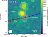 |
Fig. 1 Maximum intensity (moment 8) map of the SiO J=5–4 line at 217.105 GHz (color scale and white contours) and continuum image (setup 1 at 225 GHz; magenta contours) in the innermost region of L483. The moment 8 image was produced using the velocity range of ±10 km s−1 with respect to the systemic velocity of 5.5 km s−1. The synthesized beam is shown in the bottom left corner of the image. Contour levels are 2, 4, and 8 times the rms noise level of 3.78 mJy beam−1 for the maximum intensity and 4, 8, 16, and 32 times the rms noise level of 0.23 mJy beam−1 for the continuum image, respectively. The 0.5′′ × 0.5′′ regions where spectra (Fig. 9) have been extracted (Table 2, Fig. A.1) are indicated by red squares. Small black plus signs show the positions of continuum peaks of the binary system (Cox et al. 2022). The axes of the blue and red lobes of the E–W outflow (Oya et al. 2018) with the PA of 105 degrees are plotted by solid blue and red lines, respectively. |
 |
Fig. 2 Moment maps of the SiO J =5–4 line at 217.105 GHz of L483. (Left) Maximum intensity (moment 8; black contours) and peak velocity (moment 1; color) maps in the innermost region around the continuum peak. The synthesized beam is shown in the bottom left corner of the image. Contour levels are 2, 4, and 8 times the rms noise level of 3.78 mJy beam−1. The 0.5′′ × 0.5′′ regions where spectra (Fig. 9) have been extracted (Table 2, Fig. A.1) are indicated by red squares. Small black plus signs show the positions of continuum peaks of the binary system (Cox et al. 2022). The rectangular region (1′′ × 3′′) was used to produce the PV diagram in the north-south direction (Fig. 8). (Middle) Same image as is presented in the left panel but showing the larger image size. A black square at the image center indicates the blow-up region for the left panel. We note that the color scales of the moment 1 maps are different from those in Figs. 4–7 in order to clarify the larger velocity width of the SiO line than those of the others. (Right) Integrated intensity (moment 0; white contours) and maximum intensity (moment 8; color) images. Contour levels are 2, 4, 8, and 16 times the rms noise level of 12.67 mJy beam−1 km s−1. |
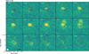 |
Fig. 3 Channel maps of the SiO J=5–4 line at 217.105 GHz for the zoom-in view. The central velocity of each panel is indicated in the top left corner. Contour levels are 4, 8, 16, 32, … times the rms noise level of 0.93 mJy beam−1. |
4.2 Localized SiO distribution in and around the outflow
On a larger scale, the SiO emission is weak and very localized in the maximum intensity map up to 2400 au from the continuum position (middle and right panels of Fig. 2). These emission components are distributed over a more extended region than the image fields of previous ALMA observations (Oya et al. 2017, 2018). Positions of the SiO emission identified in this study are labeled in Fig. 2 and Table 2 (Fig. A.1 for large-scale structures). They are located within more extended emission of SO, CS, and C18O, as is seen in the middle and right panels of Figs. 4–7. These weak SiO emission components are marginally seen in the integrated intensity (moment 0) map, while they are significant in the maximum intensity (moment 8) image (right panel of Fig. 2). In fact, they are clearly detected in the spectrum integrated over each emission region of 0.5′′ × 0.5′′ area (Fig. 9). The line profiles, peak velocities, and linewidths of the SiO spectra are consistent with those of the SO lines (Tables C.1 and C.2), and hence the detections of the SiO lines are reliable. It is unlikely that the SiO emission is resolved out because we employed the compact configurations of ALMA to achieve the maximum recoverable scale of 9.4′′, as is demonstrated for other molecular lines (Figs. 6 and 7).
The SiO linewidths at positions of these weak emission are typically ∼1 km s−1 and narrower than those in the central part, the continuum peak, SiO-peak, and SiO-N, as is summarized in Table C.1. Similar narrow SiO linewidths have been detected in other star-forming regions such as NGC1333, L1448-mm, L1448-IRS3, NGC2264, and IRAS 15398–3359 (Lefloch et al. 1998; Codella et al. 1999; Jiménez-Serra et al. 2004, 2005; López-Sepulcre et al. 2016; Okoda et al. 2021b; De Simone et al. 2022) and toward the infrared dark cloud G035.39–00.33 (Jiménez-Serra et al. 2010).
Among the identified SiO emission components, the largest one is a blueshifted feature located at 2400 au northeast of the map center, denoted as the northeastern cloud (NE-cloud). The NE-cloud is also seen in the maximum intensity maps of the lower-excitation SO NJ = 56−45 line and CS line (Figs. 4 and 6). It is an isolated emission feature north of the outflow lobe traced by more extended CS emission (Oya et al. 2017), as can be seen in Fig. 6. There is no sign of C18O emission around the NE-cloud region (Fig. 7). The fact that only shock tracers are detected toward this region would support a shock origin.
We note that the lower-excitation SO JN = 56−45 line shows a blueshifted blob at 10′′ northwest of the continuum peak (NW-blob). However, it is not detected in the SiO line in either the maximum intensity image (Fig. 2) or the integrated spectrum (Fig. 9).
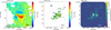 |
Fig. 4 Moment maps of the SO NJ = 56−45 line at 219.949 GHz, same as Fig. 2. Contour levels are 2, 4, 8, and 16 times the rms noise level of 5.02 mJy beam −1 for the maximum intensity (moment 8; left and middle panels) and 2, 4, 8, 16, and 32 times the rms noise level of 17.10 mJy beam−1 km s−1 for the integrated intensity map (moment 0; right panel). We note that the velocity range shown in the color scale is narrower than those of SiO (Fig. 2). |
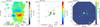 |
Fig. 5 Same as Fig. 4 but for the SO NJ = 66−55 line at 258.256 GHz. Contour levels are 2, 4, 8, and 16 times the rms noise level of 5.04 mJy beam−1 for the maximum intensity (moment 8; left and middle panels) and 2, 4, 8, 16, and 32 times the rms noise level of 17.38 mJy beam−1 km s−1 for the integrated intensity map (moment 0; right panel). |
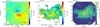 |
Fig. 6 Same as Fig. 4 but for the CS J = 5–4 line at 244.936 GHz. Contour levels are 2, 4, 8, 16, and 32 times the rms noise level of 5.13 mJy beam−1 for the maximum intensity (moment 8; left and middle panels) and 2, 4, 8, 16, 32, and 64 times the rms noise level of 16.39 mJy beam−1 km s−1 for the integrated intensity map (moment 0; right panel). |
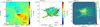 |
Fig. 7 Same as Fig. 4 but for the C18O J =2–1 line at 219.560 GHz. Contour levels are 2, 4, and 8 times the rms noise level of 4.20 mJy beam−1 for the maximum intensity (moment 8; left and middle panels) and 2, 4, and 8 times the rms noise level of 14.26 mJy beam−1 km s−1 for the integrated intensity map (moment 0; right panel). |
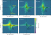 |
Fig. 8 Position-velocity (PV) maps in the north-south direction for all lines integrated with the 1′′ width. The noise levels range from 0.9 mJy to 1.7 mJy. Contour levels are common with 1, 2, 4, 8, … times 5 mJy (3–5 σ levels). A vertical and horizontal line indicate the map center and the systemic velocity (VLSR = 5.5 km s−1), respectively. The SiO PV maps (black contours) are plotted in all panels for comparison. |
4.3 Molecular abundances
Using the line parameters determined by the Gaussian fitting to the integrated spectra, molecular column densities were derived; they are listed in Table 3. For the following analysis, line frequencies, excitation energy levels, and Einstein A-coefficients were taken from the CDMS2 (Cologne Database for Molecular Spectroscopy; Müller et al. 2001). In this section, we focus on SiO and SO as shock tracers and C18O as a standard molecule tracing the gas column density. It should be noted that we compare the molecular abundances in the observed SiO emitting regions, but it is possible that each molecule traces a different gas region. In fact, the velocity widths used to derive the molecular column densities are different from molecule to molecule, as is listed in Tables C.1, C.2, and C.3, suggesting the chemical differentiation even within the same line of sight.
First, we analyzed the two SO transitions to determine the excitation temperatures, Tex, and column densities, N, assuming LTE (local thermodynamic equilibrium) and optically thin conditions. In the LTE approximation, the gas column density and the excitation temperature were derived from the best fit analysis. The SO flux uncertainties have an impact on the derivation of the excitation temperature and the column density, whose resultant uncertainties are typically 10–20% and 20–40%, respectively. For the NE-cloud region, the signal-to-noise ratio of the SO 66–55 line is about 3σ, which means that the line is marginally detected, as can be seen in Fig. 9. Thus, the uncertainty in the derived column density is larger for this region.
Next, the column densities of SiO and C18O were evaluated under the assumption of LTE conditions by using the excitation temperature derived from SO. The excitation temperature depends on the kinetic temperature, the gas density, and the spectroscopic properties of the molecule, including the Einstein coefficients and collision rates. In other words, SO, SiO, and C18O probably have different excitation temperatures in principle. However, only one line was observed for SiO and C18O, and therefore we have no information about their excitation conditions. The derived molecular abundances rely on the hypothesis that the excitation temperatures of the different molecules are similar, and adopting the excitation temperature of SO is a simplifying hypothesis.
Based on Fig. 9, there is no evidence of a narrow line component in the spectrum of the SiO line at the SiO-peak. Thus, we could only provide the upper limit (1σ) for the narrow spectral component as it cannot be distinguished from the broad component in the Gaussian fitting (Sect. 4.1). The column density of C18O at the NE-cloud position is an upper limit as the line is not detected.
The uncertainties in the molecular column densities are estimated to be 10% from the Gaussian fitting errors (± 1 σ). We confirmed that changes in the assumed excitation temperatures within the ranges of their uncertainties of the SO data are smaller than ∼20%. However, the uncertainties could be much larger because of a limited number of SO transitions employed in the LTE analysis to estimate the excitation temperatures. Furthermore, the assumption that all of SiO, SO, and C18O are emitted from the same gas is not always valid as they show different spatial distributions in the moment maps (Figs. 2, 4–7) and different line profiles even toward the same positions (Fig. 9). If we assume higher excitation temperatures of 50 K and 100 K (e.g., Podio et al. 2021; Codella et al. 2024) than those from the SO data for the central part, the estimated SiO column densities are larger by factors of about 1.0–1.1 and 1.5–1.6, respectively, for all of the Continuum peak, SiO-peak, and SiO-N positions due to the larger partition function in the higher temperature condition. On the other hand, we also compared the column densities in the outer regions (NE-cloud and other blobs) assuming the excitation temperature of 50 K and 100 K. We find that the estimated SiO column densities are changed by factors of 0.4–1.0 and 0.5–1.5, respectively. In some cases, the higher excitation temperature gives the lower optical depth for the observed transition which reduces the total column density even with the larger partition function at the higher temperature. Thus, the possible uncertainties in the SiO column densities caused by the assumed excitation temperatures would be smaller than a factor of 2.
C18O was used to estimate the H2 column densities, assuming the C18O/H2 ratio of 1.7×10⁻⁷ (Frerking et al. 1982). As was mentioned above, we simply assume that SiO, SO, and C18O are emitted from the same gas. Thus, the H2 column densities derived above only provide us with rough estimates of the SiO and SO fractional abundances relative to H2.
The SiO abundances relative to H2 are on the order of (2–3)×10−10, except at the SiO-peak, where the abundance reaches 10−9. The SiO abundance estimates are in agreement with the conclusions of Tafalla et al. (2000), who estimate maximum abundances of 8×10⁻¹⁰ in the outflow of L483. At the NE-cloud where the C18O line is not detected, we give only the lower limit for the SiO abundance (1σ) in Table 3. However, the minimum abundance reported for SiO(2.6×10⁻⁸) is very high. Because the CO distribution could be more extended than the maximum recoverable scale, the derived C18O abundance (upper limit) could be significantly affected by missing flux of the C18O line, which is possibly resolved out with the present ALMA observations.
Apart from the NE-cloud, the SiO abundances detected in our work are in agreement with the results of Lefloch et al. (1998); Codella et al. (1999); Jiménez-Serra et al. (2004, 2005, 2010); López-Sepulcre et al. (2016); De Simone et al. (2022), who all found low abundances of 10−11−10−8 in the low-velocity gas of other star-forming regions. The SiO abundances in L483 are intermediate between those in strongly shocked regions of 10−9−10−6 (Mikami et al. 1992; Martín-Pintado et al. 1992; Bachiller & Pérez Gutiérrez 1997; Jiménez-Serra et al. 2005; Cabrit et al. 2007; Lee et al. 2010; Ospina-Zamudio et al. 2019; Podio et al. 2021) and quiescent clouds with <10−12 (Ziurys et al. 1989; Jiménez-Serra et al. 2004, 2005). Thus, SiO abundances in L483 are found to be affected by shock interaction.
The SO abundances relative to H2 are about 10−9−10−8, except for those at the NE-cloud position. As was discussed for SiO, the lower-limit of the SO abundance at the NE-cloud region gives a very high value of >1.4×10⁻⁷. It could also be affected by the missing flux of the C18O line. The SO abundances in the SiO peak positions (Table 3) tend to be higher than those in the Perseus, Taurus, and Orion molecular clouds, which range from 7.3×10⁻¹⁰ to 2.0×10⁻⁹ (Rodríguez-Baras et al. 2021). Although the observed SO abundances in L483 are lower than those in strongly shocked regions (e.g., SO/H2 ∼10−8−10−6; Martín-Pintado et al. 1992; Bachiller & Pérez Gutiérrez 1997; Jiménez-Serra et al. 2005; Ospina-Zamudio et al. 2019; Podio et al. 2021; Codella et al. 2024), the relatively high abundances of SO also support a shock origin (Pineau des Forets et al. 1993).
The excitation temperatures in the localized SiO emission away from the central continuum peak tend to be lower than those in the continuum, SiO-peak, and SiO-N positions. The fact that the excitation temperature of SO is higher in the continuum peak is probably due to the higher dust and gas excitation conditions close to the binary protostellar system, as is commonly observed. In strong shock regions where SiO and SO are enhanced, gas is generally heated up to ∼100 K or higher (Podio et al. 2021; Codella et al. 2024). Thus, the outflow shock possibly contributes to the relatively high SO temperature at the SiO-peak and SiO-N positions.
The excitation temperature at the position of the NE-cloud region is the lowest, 11.3 K, due to the only marginal detection of the higher excitation SO line. This is probably due to the non-LTE excitation of the line induced by the lower H2 gas densities found at the outer parts of the molecular envelope compared to the central parts. It is almost the same as those in quiescent prestellar cores of 10 K. We note that the actual gas kinetic temperatures could be higher than the derived excitation temperatures determined by assuming the LTE conditions. To check the validity of the derived column densities and excitation temperatures, we also conducted a non-LTE analysis, which is discussed in Appendix D. Except for the results of W-blob, the derived column densities and excitation temperatures are consistent within 10%–20% (Tables 3 and D.1).
 |
Fig. 9 Spectra of all lines integrated over 0.5′′ × 0.5′′ region toward the selected positions (Table 2), as indicated in the moment maps of SiO (Fig. 2). Top 3 panels are the spectra in the central part of L483 while bottom 6 panels show those in the SiO blobs and the NE-cloud region. Considering the different flux levels between the central part (upper 3 rows) and others (lower 6 rows), different plotting ranges are employed. Vertical lines indicate the systemic velocity of VLSR = 5.5 km s−1. Gaussian fitting results are overlaid with thin red curves (Tables C.1–C.3). |
Column densities and abundances of SiO, SO, and C18O based on LTE analysis.
5 Discussion
5.1 Possible origins of SiO-peak and SiO-N emission
In L483, the SiO emission close to the continuum source shows spatial (Fig. 2) and velocity (Fig. 8) structures different from those of the SO, CS, and C18O lines. Previous principal component analysis of the spectral data cube of various molecular lines in L483 has suggested that SiO shows different characteristics from other molecular lines mostly tracing the rotating envelope and/or disk system (Okoda et al. 2021a). Thus, our result supports the idea that the strong SiO-peak is not emitted from the rotating envelope traced by the SO, CS, and C18O lines but from the outflow (Oya et al. 2017).
In this section, we consider the following possible origins of SiO-peak and SiO-N emission in L483 in terms of the outflow structure, as is shown in Fig. 10. There is no evidence of a disk in L483 on scales of 18–30 au (Jacobsen et al. 2019; Cox et al. 2022), which is smaller than the binary separation of 34 au (Cox et al. 2022). Furthermore, the existence of a circumbinary disk in L483 is still unclear. Thus, we mainly consider outflows driven by circumstellar disks associated with binary components which are unresolved with the currently achieved spatial resolution.
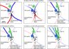 |
Fig. 10 Possible scenarios for outflows in the central region of L483. Each panel shows the same region as in the left panel of Fig. 2 with the image size of 3.2′′×3.2′′(640 au) but the image center is defined as the middle of the two continuum peaks of binary components A and B (Cox et al. 2022). Positions of SiO-peak, SiO-N, two continuum peaks A and B are indicated by crosses. Blue- and redshifted lobes of the parabolic outflow models (Oya et al. 2018) are overlaid with blue and red curves, respectively. Possible configurations of outflows (bold solid or dashed red, blue, and green lines), circumbinary disk (dashed ellipse) and circumstellar disks (small solid ellipses) are also plotted. A scale bar of 100 au is indicated in the top left panel a while sizes and directions (orientation and inclination) of disks and outflows are arbitrary. We note that the circumbinary disk with the diameter of >30 au has not been confirmed yet, as is plotted by a dashed black ellipse (Jacobsen et al. 2019; Cox et al. 2022). |
5.1.1 (a) Cavity wall of E–W outflow
A simple interpretation is that the SiO-peak and SiO-N emission are part of the E–W bipolar outflow (Fig. 10a). The E–W outflow traced by the CS line has an edge-on geometry with an inclination angle of ∼80 degrees, where the western lobe is blueshifted (Oya et al. 2018). It seems opposite to the blueshifted SiO-peak emission located at the northeastern side of the continuum source. If this is the case, the SiO-peak and SiO-N emission could trace the high-density clumps in the cavity wall of the outflow with a wide opening angle (i.e., the parabolic outflow model by Oya et al. 2018, as shown in Fig. 10a), where the swept-up gas by the outflow would be interacting with the ambient matters. The blueshifted SiO and SO emission on the southeastern side of the continuum peak could also be explained by a part of the wide opening angle cavity. Because there is no evidence of a disk in L483 with a size down to 18–30 au (Jacobsen et al. 2019; Cox et al. 2022), it is likely that the E–W outflow could be launched from one of the circumstellar disks.
5.1.2 (b) Base of E–W rotating outflow
While the velocity and position of the SiO-peak are significantly shifted with respect to those of SO, CS, and C18O lines, the blueshifted emission is detected in the northern part of the rotating envelope. If the molecular line emission traces the outflow launching region (Fig. 10b), it sometimes shows a rotation (Bjerkeli et al. 2016; Hirota et al. 2017; Lee et al. 2017; Tabone et al. 2017; Zhang et al. 2018) with the velocity close to the Keplerian rotation at the launching radius in the disk (Machida et al. 2008). The maximum velocity offset at the SiO-peak at VLSR ∼ − 1.5 km s−1(∼ −7 km s−1 with respect to the systemic velocity of 5.5 km s−1; Figs. 3 and 8) corresponds to the Keplerian rotation at the radius of 4 au, assuming the larger estimated mass of 0.2 M⊙ (Oya et al. 2017). Even for the peak velocity at the SiO-peak of VLSR ∼2.7 km s−1(∼ −3 km s−1 with respect to the systemic velocity; Table C.1), the corresponding radius is 20 au. As the SiO-N position is 400 au (2′′) away from the continuum source and is close to the systemic velocity, it would trace part of the envelope interacting with the outflow or accreting materials.
5.1.3 (c) Reorientation of outflow
Since the directions of the SiO-peak and SiO-N are approximately perpendicular to the E–W larger-scale outflow (Fig. A.1), these two SiO emission components could trace another outflow toward the northern direction (Fig. 10c). One of the possible origins is that the SiO-peak and SiO-N trace the outflow with reorientation of the flow axis due to a misalignment of the magnetic field and rotation axis (Matsumoto & Tomisaka 2004; Hirano et al. 2020; Machida et al. 2020). Because outflows are expected to be launched parallel to the rotation axis (e.g., Machida et al. 2020), the rotation axis of a circumstellar disk driving the outflow would have been changed from the eastwest direction to the north-south direction. It should be noted that the apparent separation of the binary sources are aligned in the southeast-northwest direction (Cox et al. 2022) and the direction toward the SiO-peak is almost perpendicular to the binary separation (Fig. 2). Furthermore, there is evidence of a velocity gradient in the SiO emission in Fig. 3, in the direction perpendicular to the axis of the two protostars.
Although the inclination angle of the outflow is unknown, dynamical timescales of compact outflow emission traced by the SiO-peak and SiO-N components are estimated to be 200/tan ip yr and 2000/tan iN yr, respectively, where ip and iN are the inclination angles of outflow directions toward the SiO-peak and SiO-N, respectively (inclination=90 degrees for an edge-on geometry; Eq. (B.1)). The apparent difference of dynamical timescales by a factor 10 can be caused by the different radial velocities. There are uncertainties in these timescales due to the unknown inclination angles, ip and iN. Because one can see no overlap of the SiO-peak and SiO-N positions with the separation of 100 au, it is unlikely that the outflow orientation would be close to a pole-on geometry (i.e., i < 45 degrees). Thus, the SiO-peak and SiO-N component could trace a newly ejected outflow with shorter dynamical timescales than that of the E–W outflow of 3000 yr (Oya et al. 2018).
There is ample observational evidence that binary and even single protostellar systems power outflows with different physical and chemical properties toward different propagation directions (Ospina-Zamudio et al. 2018; Ospina-Zamudio et al. 2019; Tobin et al. 2019; Hara et al. 2021; Ohashi et al. 2022; Okoda et al. 2021b; Reipurth et al. 2023; Sato et al. 2023; Evans et al. 2023; Sabatini et al. 2024; Chahine et al. 2024a,b). Possible evidence of multiple outflows with reorientation has been reported for a single protostellar object, IRAS 15398–3359 (Okoda et al. 2021b), and L483 could be a similar case but for a protobinary system.
5.1.4 (d) Misaligned outflow
The misalignment of the rotation axes of circumstellar disks and binary orbit can result in misaligned outflows in binary systems (Tsukamoto & Machida 2013; Offner et al. 2016). The direction of the rotation axis, and hence the outflows, is predicted to be time-variable, as in the case of the above scenario (Fig. 10c). In this case, the outflow traced by the SiO-peak and SiO-N emission could be launched in a different direction than the E–W outflow (Fig. 10d).
5.1.5 (e) Precessing outflow
Similar to the cases (c) and (d) in Fig. 10, the outflow traced by SiO-peak and SiO-N could be explained by the precession caused by the binary orbital motion (Fig. 10e). As is discussed in Appendix B, a simple model of the precessing outflow gives a precession period. Using the observed quantities of Δ x = 40 au (Δ α = 0.2′′) and Δ vrot = Δ VLSR = −2.3 km s−1, the precession period can be calculated to be 520 yr (Eq. (B.9)).
The estimated total mass (both components) is in the range of 0.1–0.2 M⊙ (Oya et al. 2017). The observations of Cox et al. (2022) at an angular resolution of 0.09′′ resolve the binary system of L483 and put constraints of <25 au on the size of the protostellar disks. Assuming the binary separation of 34 au and the total mass of 0.2 M⊙, the orbital period of the binary system is calculated to be 400 yr (Eq. (B.10)). If we consider the lower mass of 0.1 M⊙ or the inclination of the binary orbit, the orbital period would be longer. In addition, dynamical timescales of outflows traced by the SiO-peak and SiO-N components are estimated to be <200 yr and <2000 yr, respectively (as was discussed in case (c)). Although there are large uncertainties in disk and outflow parameters, such as protostellar masses and inclination angles of the outflow and binary orbit, the precession period of the outflow, binary orbital period, and dynamical timescales of outflows seem to be consistent with one another.
5.1.6 (f) Twin outflows
The SiO-peak and SiO-N component could trace two different outflows by both circumstellar disks in the binary system as MHD simulations have predicted (Saiki & Machida 2020; Kuruwita et al. 2017; Matsumoto 2024, and Fig. 10f). In a protobinary system, high-velocity outflows up to ∼100 km s−1 are predicted to be launched in the innermost region of the circumstellar disks at ∼0.01 au (Saiki & Machida 2020). At such a high velocity, the outflow could interact with the dense materials to produce shocked gas at high temperatures (>800 K), and hence could enhance gas-phase SiO molecules (Glassgold et al. 1991; Caselli et al. 1997; Schilke et al. 1997; Gusdorf et al. 2008a,b; Tabone et al. 2020). In this case, the E–W outflow could be driven by the circumbinary disk misaligned with those of the high-velocity outflows launched from the circumstellar disks, although there is no observational evidence of the circumbinary disk with the size of 18–30 au (Jacobsen et al. 2019; Cox et al. 2022). In the channel maps of L483 (Fig. 3), the SiO emission seems to be connected to the innermost region of the continuum peak, possibly northwestern component at the blueshifted channels from −0.6 to 2.5 km s−1, but we cannot still identify the possible launching regions of these outflows. The different linewidths between the SiO-peak (5.48 km s−1) and SiO-N (1.38 km s−1) positions could be attributed to differences in inclination angles, launched radii of each outflow, or the dynamical timescale 3. Because no high-velocity SiO emission at ≫ 10 km s−1 is found in L483, it could be attributed to larger launching radii or insufficient sensitivity of the present observations to detect weaker high-velocity line wing emission. It is also likely that the large inclination angle of the outflow parallel to the sky plane (∼80 degrees) would reduce the line-of-sight velocity of the SiO line.
5.1.7 Outflow and magnetic field directions
It has been demonstrated that the outflow orientation could be significantly affected by the binary orbital motion (Tsukamoto & Machida 2013; Offner et al. 2016). According to these simulations, outflows are launched along the rotation axis of the disk which are sometimes misaligned with the magnetic field vectors, and these configurations are time-variable (Matsumoto & Tomisaka 2004; Hirano et al. 2020; Machida et al. 2020). Furthermore, recent MHD simulations predict that binary systems drive low- and high-velocity outflows from both the circumbinary disk and circumstellar disks (Machida et al. 2009; Kuruwita et al. 2017; Saiki & Machida 2020; Matsumoto 2024). Thus, we expect to see complicated structures of outflows in binary systems. A case study of such a complex outflow system has been reported for a low-mass protostellar object, Ser-emb 15 (Sato et al. 2023). Ser-emb 15 shows two continuum sources with a separation of 218 au, associated with a well-collimated primary bipolar outflow in the north-south direction and a secondary monopolar outflow lobe perpendicular to the primary outflow (Sato et al. 2023). The CepE-mm source is a nice example of a binary intermediate-mass protostellar system with both components (1200 au distance) powering high-velocity SiO outflows which propagate in perpendicular directions (Ospina-Zamudio et al. 2018).
Cox et al. (2022) suggest that the magnetic field likely played an important role in the initial collapse and binary formation in L483. According to Fig. 2 of Cox et al. (2022), the magnetic field vectors are parallel to the E–W outflow on large scales (10000 au). Cox et al. (2022) also reveal a change in magnetic field orientation in the NW-SE direction close to the continuum peak within the inner 1000 au region, which is perpendicular to the major axis of a flattened envelope (Leung et al. 2016). These results, implying the misalignment of the large-scale (10 000 au) magnetic field and the E–W outflow with respect to the small-scale (<1000 au) magnetic field and binary orbit, would be consistent with our interpretation of misaligned or reoriented outflows.
5.1.8 Summary and caveats of interpretations
As was discussed above, we considered various configurations of outflows and disks in the protobinary system of L483. Our observational results would expect any of the models presented, but there still remain some caveats to explain possible origins.
For instance, we have suggested that only one of the circumstellar disks (or protostars) might launch the outflow in some cases (Scenario (a), (b), (c)) or two outflows have different sizes and dynamical timescales even if they coexist at the same time (Scenario (d)). This could be explained by the different protostellar masses, evolutionary (accretion) phases, or time variable outflow ejection from circumstellar disks (Saiki & Machida 2020). Moreover, physical properties of the outflows traced by various molecular lines could be sometimes misinterpreted possibly due to strong chemical differentiation in outflow lobes (e.g., Ospina-Zamudio et al. 2019).
It should also be noted that SiO-peak and SiO-N trace only the blueshifted outflow lobes driven toward the northern direction in the cases of (c), (d), (e), and (f), while there is no red-shifted counterpart toward the southern region. Such monopolar or asymmetric outflows are recognized in some protostars (Sato et al. 2023, and references therein), and a significant fraction of the SiO outflows show asymmetric structures (Podio et al. 2021; Dutta et al. 2024). Monopolar outflows are also predicted by nonideal MHD simulations (e.g., Zhao et al. 2018). It can be explained by the inhomogeneous density structure where high-density gas obstacles the outflows or chemical differentiation between bipolar outflow lobes (Ospina-Zamudio et al. 2019). We note that near-infrared H2 observations toward L483 also show the asymmetric outflow structure on a larger scale where the strong emission is detected only in the blueshifted lobe, but it is due to the larger extinction in the receding redshifted lobe at the infrared wavelengths (Fuller et al. 1995; Buckle et al. 1999).
SiO is efficiently enhanced by sputtering or grain-grain collisions followed by gas-phase reactions at a gas temperature of >800 K (Glassgold et al. 1991; Caselli et al. 1997; Schilke et al. 1997; Gusdorf et al. 2008a,b; Tabone et al. 2020). If the gas density were high enough, the excitation condition of SiO would be close to LTE, and hence it would show a high excitation temperature. As was discussed in Sect. 4.3, we assumed the same excitation temperatures of SiO and SO, around 30 K. It is much lower than those in typical shocked regions associated with SiO emission at >100 K (Podio et al. 2021; Codella et al. 2024). This would suggest that the SO emission components of the continuum, SiO-peak, and SiO-N positions could be unresolved with our observations (Sect. 4.1) that yields lower brightness temperatures, and hence underestimate the excitation temperatures. It is also likely that the SiO lines have higher excitation temperature than those of SO.
The SiO linewidths in L483 are 1–8 km s−1 (Table C.1), which are smaller than those expected for the SiO-rich shocked region of >30 km s−1 (Mikami et al. 1992; Martín-Pintado et al. 1992; Lefloch et al. 1996; Bachiller & Pérez Gutiérrez 1997). This could be due to the insufficient sensitivity to detect weak high-velocity emission or the large inclination angle of the outflow parallel to the sky plane.
The estimated fractional abundances of SiO with respect to H2 in the central regions of L483, 10−10−10−9, are lower than those of typical shocked regions (Mikami et al. 1992; Martín-Pintado et al. 1992; Bachiller & Pérez Gutiérrez 1997; Jiménez-Serra et al. 2005; Cabrit et al. 2007; Lee et al. 2010; Ospina-Zamudio et al. 2019; Podio et al. 2021). According to chemical model calculations of high-velocity outflows, the SiO abundance increases under higher mass loss rate where SiO is efficiently formed in the denser gas but less destroyed by self-shielding of the stellar radiation (Glassgold et al. 1991; Tabone et al. 2020). The lower SiO abundances in L483 could be related to this trend because its evolutionary phase is close to more evolved Class I protostars (Fuller et al. 1995; Tafalla et al. 2000; Shirley et al. 2000), which have lower mass accretion, and hence mass loss rates, than typical Class 0 protostars. The SiO/H2 ratios of 10−10−10−9 in L483 agree with some of the outflow models under different physical conditions but commonly with the mass loss rate on the order of 10−6 M⊙ yr−1 or smaller (Glassgold et al. 1991; Tabone et al. 2020).
Even the largest estimated launching radius of 20 au (0.1′′) could not be resolved with the present spectral line images. There has been no evidence of a circumbinary disk enclosing circumstellar disks associated with two protostars, which are predicted to drive the outflows (proposed for Scenario (f)). Moreover, possible evidence of circumstellar disks showing the velocity gradients have not been identified down to a scale of 18–30 au (Jacobsen et al. 2019; Cox et al. 2022). It should also be noted that the projected separation of 34 au would give a lower limit of the current separation and the actual separation and inclination of the binary orbit are unknown, and hence the estimated quantities such as the sizes and timescales of this protobinary system would have large uncertainties. Higher-resolution observations are needed to resolve the outflow launching regions in the binary system to distinguish between the different formation scenarios.
5.2 Possible origins of NE-cloud
We find a weak isolated SiO emission feature, the NE-cloud, 2400 au northeast of the central protobinary system in L483. The SiO NE-cloud region shows a narrow linewidth of 1 km s−1 at a blueshifted velocity of VLSR = 4 km s−1 (Fig. 9 and Table C.1).
Observationally, SiO is known to be enhanced in strongly shocked regions caused by high-velocity outflows with broad linewidths of >10–100 km s−1 (Mikami et al. 1992; Martín-Pintado et al. 1992; Lefloch et al. 1996; Bachiller & Pérez Gutiérrez 1997). On the other hand, some star-forming regions show narrow SiO emission with velocity widths of ∼1 km s−1, which are interpreted as (i) old outflow shocks where high-velocity components are dissipated (Lefloch et al. 1998; Codella et al. 1999; López-Sepulcre et al. 2016; Okoda et al. 2021b); (ii) a slow train of shock between an expanding bubble and ambient cloud (De Simone et al. 2022); (iii) magnetic precursor of young MHD C-shocks (Jiménez-Serra et al. 2004, 2005); or (iv) a large-scale slow shock caused by cloud-cloud collisions (Jiménez-Serra et al. 2010). Although only the lower limit of the SiO fractional abundance is derived for the NE-cloud region (Sect. 4.3), it would be in good agreement with or slightly larger than that measured in other star-forming regions showing narrow SiO emission lines, SiO/H2 ∼10−11−10−8 (Lefloch et al. 1998; Codella et al. 1999; Jiménez-Serra et al. 2004, 2005, 2010; López-Sepulcre et al. 2016; De Simone et al. 2022). Thus, the origin of SiO in the NE-cloud regions could be explained by a similar scenario.
As was introduced in the previous section, the single low-mass protostar IRAS 15398–3359 shows evidence of reorientation of the outflow (Okoda et al. 2021b). In this source, an arc-like structure of the SiO emission is extending farther than ∼1200 au and is connected to a secondary bipolar outflow perpendicular to the primary bipolar outflow. The arc-like structure has a narrow linewidth, which is interpreted as an old outflow shock where the high-velocity component has been dissipated (Lefloch et al. 1998; Codella et al. 1999; Okoda et al. 2021b).
For L483, we consider the same scenario: that the SiO NE-cloud region could be originated from a remnant of a past outflow. As is discussed by Okoda et al. (2021b) in the case of IRAS 15398–3359, the dynamical timescale would have to be shorter than the depletion timescale of the gas-phase SiO molecule (Bergin et al. 1998) but much longer than the dissipation timescale of high-velocity shocks (Codella et al. 1999) if the narrow-line SiO component is produced by old shock interaction. The dynamical timescale of the NE-cloud region is estimated to be 8000/tan i yr (Eq. (B.1)). As was discussed for the central SiO-peak and SiO-N emission (Sect. 5.1), the small radial velocities of the NE-cloud region could rule out the possibility of a pole-on geometry (i.e., i < 45 degrees). However, if the past outflow velocity is much faster and the higher-velocity components are dissipated, the estimated dynamical timescale would give an upper limit. The timescale for shock dissipation is roughly estimated to be 3000 yr (Eq. (B.12)) if we assume the size and velocity of the shocked region to be 200 au (1′′) and 10 km s−1, respectively. These timescales are slightly shorter than that of SiO depletion of 104 yr for the H2 number density of 105 cm−3 (Bergin et al. 1998), which is roughly consistent with our non-LTE analysis of the SO lines (Table D.1). The dynamical timescale of the E–W outflow is estimated to be 3000 yr (Oya et al. 2018). While the above discussion would have large uncertainties, all the timescales are roughly consistent with the idea that the SiO in the NE-cloud region would be a remnant of an old outflow where the high-velocity component is already dissipated but the gas-phase SiO is abundant.
We note that there is a filamentary gas distribution toward the southwestern direction in the maximum intensity map of CS (Fig. 6), labeled as the SW filament (Fig. A.1). The SW filament is located nearly in the opposite side of the SiO NE-cloud region with respect to the continuum peak, as is seen in the CS map, and hence it could be a counterpart of the bipolar outflow lobe. It is worth mentioning that the PA toward the NE-cloud at a scale of >1000 au would be roughly coincident with that of the SiO-peak at the much smaller scale of 100 au. Thus, the possible origins of the NE-cloud region would be related to the scenario (c), (d), (e), or (f) discussed in Sect. 5.1. Although the relationship between the central SiO emission (SiO-peak and SiO-N), NE-cloud, and SW filament is still unclear, the complex SiO distribution in L483 could reflect active events caused by the past outflow ejection and their launching mechanisms.
5.3 Possible origins of other localized SiO blobs away from the central protobinary system
In addition to the NE-cloud, there are localized compact SiO blobs which are away from the central protobinary system. These blobs are located in the outflow cavity walls mainly traced by the SO emission (Figs. 4 and 5). In fact, some of the SiO blobs are coincident with the outline of the parabolic outflow model (Oya et al. 2018), as is indicated in Fig. A.1. This suggests that the SiO blobs would be produced by shock interaction in the high-density clumps in the E–W outflow cavity wall. The timescale of shock dissipation (∼3000 yr) and gas-phase SiO depletion (∼104 yr) would be consistent with this scenario if these shocked regions are produced ∼104 yr ago, which is slightly longer than the dynamical timescale of the CS outflow (∼3000 yr Oya et al. 2018).
6 Conclusions
As part of the ALMA large program FAUST, we have presented distributions of SiO emission in a newly identified protobinary system, L483. By comparing the SiO, SO, CS, and C18O lines, we studied the physical and chemical properties of several SiO emission region in L483. The key results are listed below:
Two SiO peaks, SiO-peak and SiO-N, are located ∼100 au northwest and ∼200 au north of the continuum peak, respectively. The SiO emission at the central scale of 200 au shows spatial and velocity structures different from other molecular lines of SO, CS, and C18O. In the continuum and SiO peaks, linewidths of the observed molecular species are broad (5.5–8 km s−1) due to the rotating motion;
In addition to the central part, some localized weak SiO emission components are identified away from the central protobinary system. The most prominent one is the NE-cloud, located 2400 au northwest of the protobinary system. In addition, there are some other compact SiO blobs. All of these SiO emission regions have narrow linewidths of 1 km s−1, indicating that nonthermal gas motions are minimal;
An LTE analysis of the two SO lines suggests that the gas excitation temperatures in the central part are 32.9–38.7 K, while those in the narrow-line SiO regions tend to be lower, 11.3–26.7 K. The SO and SiO abundances are estimated to be about 10−9−10−8 and 10−10−10−9, respectively. These values are intermediate between those in strongly shocked regions and quiescent clouds, and in good agreement with those in narrow-line SiO emission regions in other star-forming regions;
The directions of the position offset toward the central SiO-peak and SiO-N components with respect to the continuum position are misaligned with the larger-scale E–W bipolar outflows, 1000 au-scale magnetic field, and rotation axis of the envelope, while they appear to be aligned with those of the binary separation. These two SiO components could be interpreted as two different outflows driven from circumstellar disks associated with both binary protostars or a single outflow launched from one of the binary components;
For the NE-cloud region, a comparison of various timescales suggests that it can be interpreted as an old outflow shock where the high-velocity shock is dissipated but the gas-phase SiO still maintains a high abundance, as has been proposed for the protostellar object IRAS 15398–3359;
Other compact SiO blobs are located in the dense part of the E–W outflow cavity walls. These SiO lines could trace the densest regions of the shock interaction located in the E–W outflow cavity wall.
Acknowledgements
We would like to thank the anonymous referee for valuable comments to clarify the manuscript. This paper makes use of the following ALMA data: ADS/JAO.ALMA#2018.1.01205.L. ALMA is a partnership of ESO (representing its member states), NSF (USA) and NINS (Japan), together with NRC (Canada), MOST and ASIAA (Taiwan), and KASI (Republic of Korea), in cooperation with the Republic of Chile. The Joint ALMA Observatory is operated by ESO, AUI/NRAO and NAOJ. Data analysis were in part carried out on common use data analysis computer system at the Astronomy Data Center, ADC, of the National Astronomical Observatory of Japan. This study is supported by the MEXT/JSPS KAKENHI Grant Numbers 18H05222, 20H05845, 20H05847, and 21K13954. This project has received funding from the European Research Council (ERC) under the European Union Horizon Europe research and innovation program (grant agreement No. 101042275, project Stellar-MADE). S. V. and M.B acknowledge the support from the European Research Council (ERC) Advanced Grant MOPPEX 833460. I.J-.S acknowledges funding from grant PID2022–136814NB-I00 funded by MICIU/AEI/ 10.13039/501100011033 and by "ERDF/EU". E. B. acknowledges the contribution of the Next Generation EU funds within the National Recovery and Resilience Plan (PNRR), Mission 4 – Education and Research, Component 2 – From Research to Business (M4C2), Investment Line 3.1 – Strengthening and creation of Research Infrastructures, Project IR0000034 – "STILES – Strengthening the Italian Leadership in ELT and SKA". L.P., C.C., and E.B. acknowledge financial support under the National Recovery and Resilience Plan (NRRP), Mission 4, Component 2, Investment 1.1, Call for tender No. 104 published on 2.2.2022 by the Italian Ministry of University and Research (MUR), funded by the European Union – NextGenerationEU – Project Title 2022JC2Y93 ChemicalOrigins: linking the fossil composition of the Solar System with the chemistry of protoplanetary disks – CUP J53D23001600006 – Grant Assignment Decree No. 962 adopted on 30.06.2023 by the Italian Ministry of Ministry of University and Research (MUR). L.P., C.C., E.B., and G.S. also acknowledge the EC H2020 project "Astro-Chemical Origins" (ACO, No 811312), the PRINMUR 2020 BEYOND-2p (Astrochemistry beyond the second period elements, Prot. 2020AFB3FX), the project ASI-Astrobiologia 2023 MIGLIORA (Modeling Chemical Complexity, F83C23000800005), the INAF-GO 2023 fundings PROTO-SKA (Exploiting ALMA data to study planet forming disks: preparing the advent of SKA, C13C23000770005), the INAF-Minigrant 2022 "Chemical Origins" (P.I.: L. Podio), and the INAF-Minigrant 2023 TRIESTE ("TRacing the chemIcal hEritage of our originS: from proTostars to planEts"; PI: G. Sabatini). H.B.L. is supported by the National Science and Technology Council (NSTC) of Taiwan (Grant Nos. 111–2112-M-110–022-MY3, 113–2112-M-110–022-MY3). L.L. acknowledges the support of UNAM-DGAPA PAPIIT grants IN108324 and IN112820 and CONACYT-CF grant 263356. F.M. acknowledges funding from the European Research Council (ERC) under the European Union's Horizon Europe research and innovation program (grant agreement No. 101053020, project Dust2Planets).
Appendix A Overall structure of L483
The overall structure of L483 denoting each region and structure discussed in the present paper is illustrated in Fig. A.1. The parabolic outflow model is taken from Oya et al. (2018), where the PA of the outflow is 105 degrees.
 |
Fig. A.1 Maximum intensity (moment 8) image of the SiO 5–4 line (color scale). The white contour shows the 2σ level of the maximum intensity of the CS 5–4 line which outlines the E–W outflow lobes (Fig. 6), with the 1 σ noise level of 5.13 mJy beam−1. Positions of specific structures traced by other lines (SO and CS) are also labeled in the panel. Each region listed in Table 2 is indicated by a red square with the size of 0.5′′×0.5′′. The parabolic outflow model (Oya et al. 2018) with a PA of 105 degrees are indicated with solid red and blue lines for the red- and blueshifted lobes, respectively. The arrows indicate the directions toward the NE-cloud and SW filament. |
Appendix B Derivation of various timescales
Here we briefly summarize the derivation of the timescales discussed in Sect. 5.
Outflows are characterized by a broad velocity range. The dynamical timescale of the outflow, tdyn, is estimated as
 (B.1)
(B.1)
in which L, v, and i are the linear size of the outflow on the plane of the sky, the radial velocity of the outflow, and the inclination angle of the outflow axis (i = 90 degrees is edge-on), respectively.
Next, we consider a timescale of precession motion of the outflow. We simply assume that the outflow is aligned in the north-south direction with the edge-on geometry and ignore the correction for the inclination angle and PA of the outflow axis. In addition, if the outflow is well collimated and the opening angle can be regarded as a constant value, the trajectory of the precessing outflow can be expressed as
 (B.2)
(B.2)
 (B.3)
(B.3)
 (B.4)
(B.4)
where the x, y, and z axes are defined as the position offsets in right ascension, line of sight, and declination directions, respectively (Fig. B.1), and ω is the angular velocity of the rotation. The outflow velocity is taken as a constant, vz, as a function of distance, z, and time, t. Using Eq. (B.3), the rotation velocity can be expressed as
 (B.5)
(B.5)
We simply assume the two representative cases for the locations of SiO-peak and SiO-N, as is summarized in Fig. B.1.
 (B.6)
(B.6)
 (B.7)
(B.7)
in which tp and tn correspond to the dynamical time at the positions of SiO-peak and SiO-N, respectively. Using Eqs. (B.6) and (B.7), the precessing period can be easily derived as
 (B.8)
(B.8)
 (B.9)
(B.9)
The orbital period of the binary system is calculated to be
 (B.10)
where a and M are the separation and the total mass of the binary system, respectively.
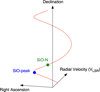 |
Fig. B.1 Geometry of the precessing outflow in L483. Here, we ignore the correction of the PA, inclination angle, and opening angle of the outflow (i.e., assuming the cylindrical north-south outflow parallel to the plane of the sky). A representative example for the positions of SiO-peak and SiO-N is indicated in the figure. |
According to Codella et al. (1999), the dissipation timescale of high-velocity components can be estimated as
 (B.11)
where ρ/ρ1 is the density ratio of the shocked gas to that of the ambient gas, r is the size of the shocked region, and v is the shock velocity. Assuming ρ/ρ1 = 10, this relationship can be expressed as
 (B.12)
Appendix C Parameters of detected lines
The line parameters determined by the Gaussian fitting at each position, the peak flux density F, brightness temperature Tb, peak LSR velocity VLSR, and FWHM (full width at half maximum) linewidth Δ VFWHM, are listed in Tables C.1, C.2, and C.3.
Line parameters of SiO J = 5–4 emission
Line parameters of SO emission
Appendix D Non-LTE analysis
For comparison, we also calculated molecular column densities using non-LTE analysis. We employed the LVG (large-velocity gradient) model (Goldreich & Kwan 1974) to estimate SO excitation temperatures Tex, optical depths τ, column density N[SO], and H2 density n[H2] for each position by a least-squares analysis. Kinetic temperatures Tkin were assumed to be 20, 30, 40, and 50 K. Because of the relatively high excitation temperatures, the LVG calculations could not converge at the kinetic temperature of 10 K for all positions, 20 K for the continuum peak, SiO-peak, SiO-N, and SE-blob positions and 30 K for the SiO-peak position. Collision rates of SO and para-H2 up to the NJ = 1010 levels (Eu = 127 K) were taken from the BASECOL data base (Dubernet et al. 2024), for which the original collisional datasets were calculated by Lique et al. (2007). The results are presented in Table D.1 for kinetic temperatures in the range 20 K–50 K, with a minimum value which depends on the sources.
Compared with the results of the LTE analysis (Table 3), difference in column densities and excitation temperatures determined by the non-LTE analysis are ∼10–20%. One exception is the results for W-blob, in which the excitation temperature derived from the non-LTE analysis are smaller by a factor of 2 but the column density is larger by a factor of 3 than those from the LTE analysis. Because the derived excitation temperature and column density are more sensitive to the integrated intensity ratios and brightness temperature ratios in the LTE and non-LTE (LVG) analysis, respectively, the different linewidths for two SO transitions affects the results, in particular for W-blob (Table C.2).
Line parameters of C18O J = 2–1 emission
Non-LTE analysis for the SO lines
References
- Agúndez, M., Marcelino, N., Cernicharo, J., et al. 2019, A&A, 625, A147 [NASA ADS] [CrossRef] [EDP Sciences] [Google Scholar]
- Alves, F. O., Girart, J. M., Caselli, P., et al. 2017, A&A, 603, L3 [NASA ADS] [CrossRef] [EDP Sciences] [Google Scholar]
- Bachiller, R., & Pérez Gutiérrez, M. 1997, ApJ, 487, L93 [Google Scholar]
- Bally, J. 2016, ARA&A, 54, 491 [Google Scholar]
- Bergin, E. A., Melnick, G. J., & Neufeld, D. A. 1998, ApJ, 499, 777 [Google Scholar]
- Bjerkeli, P., van der Wiel, M. H. D., Harsono, D., et al. 2016, Nature, 540, 406 [NASA ADS] [CrossRef] [Google Scholar]
- Buckle, J. V., Hatchell, J., & Fuller, G. A. 1999, A&A, 348, 584 [NASA ADS] [Google Scholar]
- Cabrit, S., Codella, C., Gueth, F., et al. 2007, A&A, 468, L29 [NASA ADS] [CrossRef] [EDP Sciences] [Google Scholar]
- CASA Team (Bean, B., et al.) 2022, PASP, 134, 114501 [NASA ADS] [CrossRef] [Google Scholar]
- Caselli, P., Hartquist, T. W., & Havnes, O. 1997, A&A, 322, 296 [NASA ADS] [Google Scholar]
- Cazaux, S., Tielens, A. G. G. M., Ceccarelli, C., et al. 2003, ApJ, 593, L51 [CrossRef] [Google Scholar]
- Ceccarelli, C., Caselli, P., Herbst, E., et al. 2007, Protostars and Planets V, 47 [Google Scholar]
- Ceccarelli, C., Caselli, P., Fontani, F., et al. 2017, ApJ, 850, 176 [NASA ADS] [CrossRef] [Google Scholar]
- Ceccarelli, C., Codella, C., Balucani, N., et al. 2023, Astron. Soc. Pac. Conf. Ser., 534, 379 [NASA ADS] [Google Scholar]
- Chahine, L., Ceccarelli, C., De Simone, M., et al. 2024a, MNRAS, 531, 2653 [NASA ADS] [Google Scholar]
- Chahine, L., Ceccarelli, C., De Simone, M., et al. 2024b, MNRAS, 534, L48 [NASA ADS] [Google Scholar]
- Codella, C., Bachiller, R., & Reipurth, B. 1999, A&A, 343, 585 [NASA ADS] [Google Scholar]
- Codella, C., Cabrit, S., Gueth, F., et al. 2007, A&A, 462, L53 [NASA ADS] [CrossRef] [EDP Sciences] [Google Scholar]
- Codella, C., Ceccarelli, C., Chandler, C., et al. 2021, Front. Astron. Space Sci., 8, 227 [NASA ADS] [CrossRef] [Google Scholar]
- Codella, C., Podio, L., De Simone, M., et al. 2024, MNRAS, 528, 7383 [NASA ADS] [CrossRef] [Google Scholar]
- Cox, E. G., Novak, G., Sadavoy, S. I., et al. 2022, ApJ, 932, 34 [NASA ADS] [CrossRef] [Google Scholar]
- Dame, T. M., & Thaddeus, P. 1985, ApJ, 297, 751 [NASA ADS] [CrossRef] [Google Scholar]
- De Simone, M., Codella, C., Ceccarelli, C., et al. 2022, MNRAS, 512, 5214 [CrossRef] [Google Scholar]
- Dubernet, M. L., Boursier, C., Denis-Alpizar, O., et al. 2024, A&A, 683, A40 [NASA ADS] [CrossRef] [EDP Sciences] [Google Scholar]
- Duchêne, G., & Kraus, A. 2013, ARA&A, 51, 269 [Google Scholar]
- Dutta, S., Lee, C.-F., Johnstone, D., et al. 2024, AJ, 167, 72 [Google Scholar]
- Evans, L., Vastel, C., Fontani, F., et al. 2023, A&A, 678, A160 [NASA ADS] [CrossRef] [EDP Sciences] [Google Scholar]
- Frank, A., Ray, T. P., Cabrit, S., et al. 2014, Protostars and Planets VI, 451 [Google Scholar]
- Frerking, M. A., Langer, W. D., & Wilson, R. W. 1982, ApJ, 262, 590 [Google Scholar]
- Fuller, G. A., Lada, E. A., Masson, C. R., et al. 1995, ApJ, 453, 754 [Google Scholar]
- Goldreich, P., & Kwan, J. 1974, ApJ, 189, 441 [CrossRef] [Google Scholar]
- Glassgold, A. E., Mamon, G. A., & Huggins, P. J. 1991, ApJ, 373, 254 [NASA ADS] [CrossRef] [Google Scholar]
- Gusdorf, A., Cabrit, S., Flower, D. R., et al. 2008a, A&A, 482, 809 [NASA ADS] [CrossRef] [EDP Sciences] [Google Scholar]
- Gusdorf, A., Pineau Des Forêts, G., Cabrit, S., et al. 2008b, A&A, 490, 695 [NASA ADS] [CrossRef] [EDP Sciences] [Google Scholar]
- Hara, C., Kawabe, R., Nakamura, F., et al. 2021, ApJ, 912, 34 [NASA ADS] [CrossRef] [Google Scholar]
- Hirano, S., Tsukamoto, Y., Basu, S., et al. 2020, ApJ, 898, 118 [NASA ADS] [CrossRef] [Google Scholar]
- Hirota, T., Ohishi, M., & Yamamoto, S. 2009, ApJ, 699, 585 [Google Scholar]
- Hirota, T., Sakai, N., & Yamamoto, S. 2010, ApJ, 720, 1370 [Google Scholar]
- Hirota, T., Machida, M. N., Matsushita, Y., et al. 2017, Nat. Astron., 1, 0146 [Google Scholar]
- Jacobsen, S. K., Jørgensen, J. K., Di Francesco, J., et al. 2019, A&A, 629, A29 [NASA ADS] [CrossRef] [EDP Sciences] [Google Scholar]
- Jiménez-Serra, I., Martín-Pintado, J., Rodríguez-Franco, A., et al. 2004, ApJ, 603, L49 [CrossRef] [Google Scholar]
- Jiménez-Serra, I., Martín-Pintado, J., Rodríguez-Franco, A., et al. 2005, ApJ, 627, L121 [CrossRef] [Google Scholar]
- Jiménez-Serra, I., Caselli, P., Tan, J. C., et al. 2010, MNRAS, 406, 187 [Google Scholar]
- Jørgensen, J. K. 2004, A&A, 424, 589 [NASA ADS] [CrossRef] [EDP Sciences] [Google Scholar]
- Kuruwita, R. L., Federrath, C., & Ireland, M. 2017, MNRAS, 470, 1626 [NASA ADS] [CrossRef] [Google Scholar]
- Lee, C.-F., Hasegawa, T. I., Hirano, N., et al. 2010, ApJ, 713, 731 [NASA ADS] [CrossRef] [Google Scholar]
- Lee, C.-F., Ho, P. T. P., Li, Z.-Y., et al. 2017, Nat. Astron., 1, 0152 [CrossRef] [Google Scholar]
- Lefloch, B., Eisloeffel, J., & Lazareff, B. 1996, A&A, 313, L17 [NASA ADS] [Google Scholar]
- Lefloch, B., Castets, A., Cernicharo, J., et al. 1998, ApJ, 504, L109 [NASA ADS] [CrossRef] [Google Scholar]
- Leung, G. Y. C., Lim, J., & Takakuwa, S. 2016, ApJ, 833, 55 [Google Scholar]
- Lique, F., Senent, M.-L., Spielfiedel, A., et al. 2007, J. Chem. Phys., 126, 164312 [NASA ADS] [CrossRef] [Google Scholar]
- López-Sepulcre, A., Watanabe, Y., Sakai, N., et al. 2016, ApJ, 822, 85 [CrossRef] [Google Scholar]
- Machida, M. N., Inutsuka, S. & Matsumoto, T. 2008, ApJ, 676, 1088 [CrossRef] [Google Scholar]
- Machida, M. N., Inutsuka, S. & Matsumoto, T. 2009, ApJ, 704, L10 [NASA ADS] [CrossRef] [Google Scholar]
- Machida, M. N., Hirano, S., & Kitta, H. 2020, MNRAS, 491, 2180 [Google Scholar]
- Martín-Pintado, J., Bachiller, R., & Fuente, A. 1992, A&A, 254, 315 [Google Scholar]
- Matsumoto, T. 2024, ApJ, 964, 133 [Google Scholar]
- Matsumoto, T., & Tomisaka, K. 2004, ApJ, 616, 266 [NASA ADS] [CrossRef] [Google Scholar]
- Mikami, H., Umemoto, T., Yamamoto, S., et al. 1992, ApJ, 392, L87 [Google Scholar]
- Müller, H. S. P., Thorwirth, S., Roth, D. A., et al. 2001, A&A, 370, L49 [Google Scholar]
- Myers, P. C., Bachiller, R., Caselli, P., et al. 1995, ApJ, 449, L65 [NASA ADS] [Google Scholar]
- Offner, S. S. R., Dunham, M. M., Lee, K. I., et al. 2016, ApJ, 827, L11 [Google Scholar]
- Ohashi, S., Codella, C., Sakai, N., et al. 2022, ApJ, 927, 54 [NASA ADS] [CrossRef] [Google Scholar]
- Okoda, Y., Oya, Y., Abe, S., et al. 2021a, ApJ, 923, 168 [Google Scholar]
- Okoda, Y., Oya, Y., Francis, L., et al. 2021b, ApJ, 910, 11 [Google Scholar]
- Ospina-Zamudio, J., Lefloch, B., Ceccarelli, C., et al. 2018, A&A, 618, A145 [NASA ADS] [CrossRef] [EDP Sciences] [Google Scholar]
- Ospina-Zamudio, J., Lefloch, B., Favre, C., et al. 2019, MNRAS, 490, 2679 [NASA ADS] [CrossRef] [Google Scholar]
- Oya, Y. 2020, Origins: From the Protosun to the First Steps of Life, 345, 111 [Google Scholar]
- Oya, Y., Sakai, N., Watanabe, Y., et al. 2017, ApJ, 837, 174 [Google Scholar]
- Oya, Y., Sakai, N., Watanabe, Y., et al. 2018, ApJ, 863, 72 [NASA ADS] [CrossRef] [Google Scholar]
- Oya, Y., Watanabe, Y., López-Sepulcre, A., et al. 2021, ApJ, 921, 12 [NASA ADS] [CrossRef] [Google Scholar]
- Park, Y.-S., Panis, J.-F., Ohashi, N., et al. 2000, ApJ, 542, 344 [Google Scholar]
- Pascucci, I., Cabrit, S., Edwards, S., et al. 2023, Protostars and Planets VII, 534, 567 [NASA ADS] [Google Scholar]
- Pineau des Forets, G., Roueff, E., Schilke, P., et al. 1993, MNRAS, 262, 915 [CrossRef] [Google Scholar]
- Podio, L., Tabone, B., Codella, C., et al. 2021, A&A, 648, A45 [NASA ADS] [CrossRef] [EDP Sciences] [Google Scholar]
- Pudritz, R. E., & Ray, T. P. 2019, Front. Astron. Space Sci., 6, 54 [Google Scholar]
- Reipurth, B., Bally, J., Yen, H.-W., et al. 2023, AJ, 165, 209 [Google Scholar]
- Rodríguez-Baras, M., Fuente, A., Riviére-Marichalar, P., et al. 2021, A&A, 648, A120 [NASA ADS] [CrossRef] [EDP Sciences] [Google Scholar]
- Sabatini, G., Podio, L., Codella, C., et al. 2024, A&A, 684, L12 [NASA ADS] [CrossRef] [EDP Sciences] [Google Scholar]
- Saiki, Y., & Machida, M. N. 2020, ApJ, 897, L22 [NASA ADS] [CrossRef] [Google Scholar]
- Sakai, N., & Yamamoto, S. 2013, Chem. Rev., 113, 8981 [Google Scholar]
- Sakai, N., Sakai, T., Hirota, T., et al. 2009, ApJ, 697, 769 [CrossRef] [Google Scholar]
- Sakai, N., Sakai, T., Hirota, T., et al. 2014, Nature, 507, 78 [Google Scholar]
- Sato, A., Tokuda, K., Machida, M. N., et al. 2023, ApJ, 958, 102 [Google Scholar]
- Schilke, P., Walmsley, C. M., Pineau des Forets, G., et al. 1997, A&A, 321, 293 [Google Scholar]
- Shirley, Y. L., Evans, N. J., Rawlings, J. M. C., et al. 2000, ApJS, 131, 249 [NASA ADS] [CrossRef] [Google Scholar]
- Tabone, B., Cabrit, S., Bianchi, E., et al. 2017, A&A, 607, L6 [NASA ADS] [CrossRef] [EDP Sciences] [Google Scholar]
- Tabone, B., Godard, B., Pineau des Forêts, G., et al. 2020, A&A, 636, A60 [NASA ADS] [CrossRef] [EDP Sciences] [Google Scholar]
- Tafalla, M., Myers, P. C., Mardones, D., et al. 2000, A&A, 359, 967 [Google Scholar]
- Takakuwa, S., Kamazaki, T., Saito, M., et al. 2007, PASJ, 59, 1 [NASA ADS] [CrossRef] [Google Scholar]
- Tobin, J. J., Kratter, K. M., Persson, M. V., et al. 2016, Nature, 538, 483 [NASA ADS] [CrossRef] [Google Scholar]
- Tobin, J. J., Bourke, T. L., Mader, S., et al. 2019, ApJ, 870, 81 [CrossRef] [Google Scholar]
- Tsukamoto, Y., & Machida, M. N. 2013, MNRAS, 428, 1321 [NASA ADS] [CrossRef] [Google Scholar]
- Tsukamoto, Y., Maury, A., Commercon, B., et al. 2023, Protostars and Planets VII, 534, 317 [Google Scholar]
- Velusamy, T., Langer, W. D., & Thompson, T. 2014, ApJ, 783, 6 [NASA ADS] [CrossRef] [Google Scholar]
- Zhang, Y., Higuchi, A. E., Sakai, N., et al. 2018, ApJ, 864, 76 [NASA ADS] [CrossRef] [Google Scholar]
- Zhao, B., Caselli, P., Li, Z.-Y., et al. 2018, MNRAS, 473, 4868 [CrossRef] [Google Scholar]
- Ziurys, L. M., Friberg, P., & Irvine, W. M. 1989, ApJ, 343, 201 [NASA ADS] [CrossRef] [Google Scholar]
https://faust-imaging.readthedocs.io/en/latest/ (Chandler et al., in prep., Moellenbrock et al., in prep.) for more details.
It may also be possible that the different linewidths could be attributed to different levels of shock dissipation (Sect. 5.2). However, given the shorter dynamical timescales of <2000 yr for SiO-N than that of the shock dissipation of 3000 yr, this possibility may be ruled out.
All Tables
All Figures
|
Fig. 1 Maximum intensity (moment 8) map of the SiO J=5–4 line at 217.105 GHz (color scale and white contours) and continuum image (setup 1 at 225 GHz; magenta contours) in the innermost region of L483. The moment 8 image was produced using the velocity range of ±10 km s−1 with respect to the systemic velocity of 5.5 km s−1. The synthesized beam is shown in the bottom left corner of the image. Contour levels are 2, 4, and 8 times the rms noise level of 3.78 mJy beam−1 for the maximum intensity and 4, 8, 16, and 32 times the rms noise level of 0.23 mJy beam−1 for the continuum image, respectively. The 0.5′′ × 0.5′′ regions where spectra (Fig. 9) have been extracted (Table 2, Fig. A.1) are indicated by red squares. Small black plus signs show the positions of continuum peaks of the binary system (Cox et al. 2022). The axes of the blue and red lobes of the E–W outflow (Oya et al. 2018) with the PA of 105 degrees are plotted by solid blue and red lines, respectively. |
| In the text | |
|
Fig. 2 Moment maps of the SiO J =5–4 line at 217.105 GHz of L483. (Left) Maximum intensity (moment 8; black contours) and peak velocity (moment 1; color) maps in the innermost region around the continuum peak. The synthesized beam is shown in the bottom left corner of the image. Contour levels are 2, 4, and 8 times the rms noise level of 3.78 mJy beam−1. The 0.5′′ × 0.5′′ regions where spectra (Fig. 9) have been extracted (Table 2, Fig. A.1) are indicated by red squares. Small black plus signs show the positions of continuum peaks of the binary system (Cox et al. 2022). The rectangular region (1′′ × 3′′) was used to produce the PV diagram in the north-south direction (Fig. 8). (Middle) Same image as is presented in the left panel but showing the larger image size. A black square at the image center indicates the blow-up region for the left panel. We note that the color scales of the moment 1 maps are different from those in Figs. 4–7 in order to clarify the larger velocity width of the SiO line than those of the others. (Right) Integrated intensity (moment 0; white contours) and maximum intensity (moment 8; color) images. Contour levels are 2, 4, 8, and 16 times the rms noise level of 12.67 mJy beam−1 km s−1. |
| In the text | |
|
Fig. 3 Channel maps of the SiO J=5–4 line at 217.105 GHz for the zoom-in view. The central velocity of each panel is indicated in the top left corner. Contour levels are 4, 8, 16, 32, … times the rms noise level of 0.93 mJy beam−1. |
| In the text | |
|
Fig. 4 Moment maps of the SO NJ = 56−45 line at 219.949 GHz, same as Fig. 2. Contour levels are 2, 4, 8, and 16 times the rms noise level of 5.02 mJy beam −1 for the maximum intensity (moment 8; left and middle panels) and 2, 4, 8, 16, and 32 times the rms noise level of 17.10 mJy beam−1 km s−1 for the integrated intensity map (moment 0; right panel). We note that the velocity range shown in the color scale is narrower than those of SiO (Fig. 2). |
| In the text | |
|
Fig. 5 Same as Fig. 4 but for the SO NJ = 66−55 line at 258.256 GHz. Contour levels are 2, 4, 8, and 16 times the rms noise level of 5.04 mJy beam−1 for the maximum intensity (moment 8; left and middle panels) and 2, 4, 8, 16, and 32 times the rms noise level of 17.38 mJy beam−1 km s−1 for the integrated intensity map (moment 0; right panel). |
| In the text | |
|
Fig. 6 Same as Fig. 4 but for the CS J = 5–4 line at 244.936 GHz. Contour levels are 2, 4, 8, 16, and 32 times the rms noise level of 5.13 mJy beam−1 for the maximum intensity (moment 8; left and middle panels) and 2, 4, 8, 16, 32, and 64 times the rms noise level of 16.39 mJy beam−1 km s−1 for the integrated intensity map (moment 0; right panel). |
| In the text | |
|
Fig. 7 Same as Fig. 4 but for the C18O J =2–1 line at 219.560 GHz. Contour levels are 2, 4, and 8 times the rms noise level of 4.20 mJy beam−1 for the maximum intensity (moment 8; left and middle panels) and 2, 4, and 8 times the rms noise level of 14.26 mJy beam−1 km s−1 for the integrated intensity map (moment 0; right panel). |
| In the text | |
|
Fig. 8 Position-velocity (PV) maps in the north-south direction for all lines integrated with the 1′′ width. The noise levels range from 0.9 mJy to 1.7 mJy. Contour levels are common with 1, 2, 4, 8, … times 5 mJy (3–5 σ levels). A vertical and horizontal line indicate the map center and the systemic velocity (VLSR = 5.5 km s−1), respectively. The SiO PV maps (black contours) are plotted in all panels for comparison. |
| In the text | |
|
Fig. 9 Spectra of all lines integrated over 0.5′′ × 0.5′′ region toward the selected positions (Table 2), as indicated in the moment maps of SiO (Fig. 2). Top 3 panels are the spectra in the central part of L483 while bottom 6 panels show those in the SiO blobs and the NE-cloud region. Considering the different flux levels between the central part (upper 3 rows) and others (lower 6 rows), different plotting ranges are employed. Vertical lines indicate the systemic velocity of VLSR = 5.5 km s−1. Gaussian fitting results are overlaid with thin red curves (Tables C.1–C.3). |
| In the text | |
|
Fig. 10 Possible scenarios for outflows in the central region of L483. Each panel shows the same region as in the left panel of Fig. 2 with the image size of 3.2′′×3.2′′(640 au) but the image center is defined as the middle of the two continuum peaks of binary components A and B (Cox et al. 2022). Positions of SiO-peak, SiO-N, two continuum peaks A and B are indicated by crosses. Blue- and redshifted lobes of the parabolic outflow models (Oya et al. 2018) are overlaid with blue and red curves, respectively. Possible configurations of outflows (bold solid or dashed red, blue, and green lines), circumbinary disk (dashed ellipse) and circumstellar disks (small solid ellipses) are also plotted. A scale bar of 100 au is indicated in the top left panel a while sizes and directions (orientation and inclination) of disks and outflows are arbitrary. We note that the circumbinary disk with the diameter of >30 au has not been confirmed yet, as is plotted by a dashed black ellipse (Jacobsen et al. 2019; Cox et al. 2022). |
| In the text | |
|
Fig. A.1 Maximum intensity (moment 8) image of the SiO 5–4 line (color scale). The white contour shows the 2σ level of the maximum intensity of the CS 5–4 line which outlines the E–W outflow lobes (Fig. 6), with the 1 σ noise level of 5.13 mJy beam−1. Positions of specific structures traced by other lines (SO and CS) are also labeled in the panel. Each region listed in Table 2 is indicated by a red square with the size of 0.5′′×0.5′′. The parabolic outflow model (Oya et al. 2018) with a PA of 105 degrees are indicated with solid red and blue lines for the red- and blueshifted lobes, respectively. The arrows indicate the directions toward the NE-cloud and SW filament. |
| In the text | |
|
Fig. B.1 Geometry of the precessing outflow in L483. Here, we ignore the correction of the PA, inclination angle, and opening angle of the outflow (i.e., assuming the cylindrical north-south outflow parallel to the plane of the sky). A representative example for the positions of SiO-peak and SiO-N is indicated in the figure. |
| In the text | |
Current usage metrics show cumulative count of Article Views (full-text article views including HTML views, PDF and ePub downloads, according to the available data) and Abstracts Views on Vision4Press platform.
Data correspond to usage on the plateform after 2015. The current usage metrics is available 48-96 hours after online publication and is updated daily on week days.
Initial download of the metrics may take a while.