| Issue |
A&A
Volume 695, March 2025
|
|
|---|---|---|
| Article Number | A42 | |
| Number of page(s) | 23 | |
| Section | Stellar structure and evolution | |
| DOI | https://doi.org/10.1051/0004-6361/202451733 | |
| Published online | 07 March 2025 | |
A study in scarlet
I. Photometric properties of a sample of intermediate-luminosity red transients
1
INAF – Osservatorio Astronomico di Padova, Vicolo dell’Osservatorio 5, I-35122 Padova, Italy
2
INAF – Osservatorio Astronomico di Brera, Via E. Bianchi 46, 23807 Merate (LC), Italy
3
Yunnan Observatories, Chinese Academy of Sciences, Kunming 650216, PR China
4
Key Laboratory for the Structure and Evolution of Celestial Objects, Chinese Academy of Sciences, Kunming 650216, P.R. China
5
International Centre of Supernovae, Yunnan Key Laboratory Kunming 650216, PR China
6
Graduate Institute of Astronomy, National Central University, 300 Jhongda Road, 32001 Jhongli, Taiwan
7
SRON, Netherlands Institute for Space Research, Niels Bohrweg 4, 2333 CA, Leiden, The Netherlands
8
Department of Astrophysics/IMAPP, Radboud University Nijmegen, P.O. Box 9010 6500 GL, Nijmegen, The Netherlands
9
Institute of Space Sciences (ICE, CSIC), Campus UAB, Carrer de Can Magrans s/n, E-08193 Barcelona, Spain
10
School of Physics, O’Brien Centre for Science North, University College Dublin, Belfield, Dublin 4, Ireland
11
The Oskar Klein Centre, Department of Astronomy, Stockholm University, AlbaNova, 10691 Stockholm, Sweden
12
Hiroshima Astrophysical Science Center, Hiroshima University, Higashi-Hiroshima, Japan
13
Department of Physics, Florida State University, 77 Chieftan Way, Tallahassee, FL 32306, USA
14
Las Cumbres Observatory, 6740 Cortona Dr. Suite 102, Goleta, CA 93117, USA
15
Department of Physics, University of California, Santa Barbara, CA 93106, USA
16
School of Physics & Astronomy, Cardiff University, Queens Buildings, The Parade, Cardiff CF24 3AA, UK
17
INAF, Osservatorio Astronomico di Capodimonte, Salita Moiariello 16, I-80131 Napoli, Italy
18
DARK, Niels Bohr Institute, University of Copenhagen, Jagtvej 128, 2200 Copenhagen, Denmark
19
Caltech, Mail Code 220-6, Pasadena, CA 91125, USA
20
Tuorla Observatory, Department of Physics and Astronomy, University of Turku, 20014 Turku, Finland
21
Astrophysics Research Institute, Liverpool John Moores University, IC2, Liverpool Science Park, 146 Brownlow Hill, Liverpool L3 5RF, UK
22
Max-Planck-Institut für Astrophysik, Karl-Schwarzschild Str. 1, D-85748 Garching, Germany
23
Aryabhatta Research Institute of observational sciences, Manora Peak, Nainital 263001, India
24
Instituto de Alta Investigación, Universidad de Tarapacá, Casilla 7D, Arica, Chile
25
School of Physics, Trinity College Dublin, College Green, Dublin 2, Ireland
26
Steward Observatory, University of Arizona, 933 North Cherry Avenue, Tucson, AZ 85721-0065, USA
27
Department of Physics, University of Oxford, Keble Road, Oxford OX1 3RH, UK
28
Astrophysics Research Centre, School of Mathematics and Physics, Queens University Belfast Belfast BT7 1NN, UK,
29
Department of Physics and Astronomy, Aarhus University, Ny Munkegade 120, DK-8000 Aarhus C, Denmark
30
INAF – Osservatorio Astronomico d’Abruzzo, via M. Maggini snc, Teramo I-64100, Italy
31
Department of Physics, University of California, Davis, CA 95616, USA
32
European Southern Observatory, Alonso de Córdova 3107, Casilla 19, Santiago, Chile
33
Millennium Institute of Astrophysics, Nuncio Monsenor Sótero Sanz 100, Providencia, 8320000 Santiago, Chile
34
INAF-Osservatorio Astrofisico di Catania, Via Santa Sofia 78, I-95123 Catania, Italy
35
Instituto de Astrofísica, Universidad Andres Bello, Fernandez Concha 700, Las Condes, Santiago RM, Chile
36
ICRANet, Piazza della Repubblica 10, I-65122 Pescara, Italy
37
Institut für Theoretische Physik, Goethe Universität, Max-von-Laue-Str. 1, 60438 Frankfurt am Main, Germany
38
INFN-TIFPA, Trento Institute for Fundamental Physics and Applications, Via Sommarive 14, I-38123 Trento, Italy
39
Institut d’Estudis Espacials de Catalunya (IEEC), E-08034 Barcelona, Spain
40
Center for Astrophysics, Harvard & Smithsonian, Cambridge, Massachusetts, MA 02138, USA
41
The NSF AI Institute for Artificial Intelligence and Fundamental Interactions, 77 Massachusetts Avenue, Cambridge, USA
42
Finnish Centre for Astronomy with ESO (FINCA), University of Turku, Väisäläntie 20, 21500 Piikkiö, Finland
43
DTU Space, National Space Institute, Technical University of Denmark, Elektrovej 327, 2800Kgs. Lyngby, Denmark
44
Dipartimento di Fisica e Astronomia “G. Galilei”, Università degli studi di Padova Vicolo dell’Osservatorio 3, I-35122 Padova, Italy
45
IAASARS, National Observatory of Athens, Metaxa & Vas. Pavlou St., 15236 Penteli, Athens, Greece
46
Department of Astronomy, University of Virginia, Charlottesville, VA 22904, USA
47
Max-Planck-Institut für Extraterrestrische Physik, Giessenbachstraße 1, 85748 Garching, Germany
48
Department of Physics and Astronomy, University of North Carolina at Chapel Hill, Chapel Hill, NC 27599, USA
49
Cosmic Dawn Center (DAWN), Rådmandsgade 64, 2200 Copenhagen N., Denmark
50
Niels Bohr Institute, University of Copenhagen, Jagtvej 128, 2200 København N, Denmark
51
Manipal Centre for Natural Sciences, Manipal Academy of Higher Education, Manipal, – 576104 Karnataka, India
52
Indian Institute Of Astrophysics, 100 Feet Rd, Santhosapuram, 2nd Block, Koramangala, Bengaluru, Karnataka 560034, India
⋆ Corresponding author; This email address is being protected from spambots. You need JavaScript enabled to view it.
Received:
31
July
2024
Accepted:
21
January
2025
Abstract
Aims. We investigate the photometric characteristics of a sample of intermediate-luminosity red transients (ILRTs), a class of elusive objects with peak luminosity between that of classical novae and standard supernovae. Our goal is to provide a stepping stone in the path to reveal the physical origin of such events, thanks to the analysis of the datasets collected.
Methods. We present the multi-wavelength photometric follow-up of four ILRTs, namely NGC 300 2008OT-1, AT 2019abn, AT 2019ahd, and AT 2019udc. Through the analysis and modelling of their spectral energy distribution and bolometric light curves, we inferred the physical parameters associated with these transients.
Results. All four objects display a single-peaked light curve which ends in a linear decline in magnitudes at late phases. A flux excess with respect to a single blackbody emission is detected in the infrared domain for three objects in our sample, a few months after maximum. This feature, commonly found in ILRTs, is interpreted as a sign of dust formation. Mid-infrared monitoring of NGC 300 2008OT-1 761 days after maximum allowed us to infer the presence of ∼10−3–10−5 M⊙ of dust, depending on the chemical composition and the grain size adopted. The late-time decline of the bolometric light curves of the considered ILRTs is shallower than expected for 56Ni decay, hence requiring an additional powering mechanism. James Webb Space Telescope observations of AT 2019abn prove that the object has faded below its progenitor luminosity in the mid-infrared domain, five years after its peak. Together with the disappearance of NGC 300 2008OT-1 in Spitzer images seven years after its discovery, this supports the terminal explosion scenario for ILRTs. With a simple semi-analytical model we tried to reproduce the observed bolometric light curves in the context of a few solar masses ejected at few 103 km s−1 and enshrouded in an optically thick circumstellar medium.
Key words: circumstellar matter / supernovae: general / supernovae: individual: NGC 300 2008OT-1 / supernovae: individual: AT 2019abn / supernovae: individual: AT 2019ahd / supernovae: individual: AT 2019udc
© The Authors 2025
 Open Access article, published by EDP Sciences, under the terms of the Creative Commons Attribution License (https://creativecommons.org/licenses/by/4.0), which permits unrestricted use, distribution, and reproduction in any medium, provided the original work is properly cited.
This article is published in open access under the Subscribe to Open model. This email address is being protected from spambots. You need JavaScript enabled to view it. to support open access publication.
1. Introduction
It is well established that single stars with an initial mass below ∼8 M⊙ will end their lives as white dwarfs, cooling down while supported by the electron degeneracy pressure in their cores. In contrast, stars with initial masses between ∼10 M⊙ and 40 M⊙ will complete all the nuclear burning cycles and will undergo a violent explosion as their core collapses (Woosley et al. 2002). This apparently simple distinction raises the complicated question of what the exact initial mass limit is that separates the two opposite fates. Stars with a zero-age main-sequence mass between 8 M⊙ and 10 M⊙ are expected to form a degenerate O-Ne-Mg core during their lifetimes (Nomoto 1984). Such stars are labelled super-asymptotic giant branch (SAGB) stars, and the outcome of their evolution is uncertain. If the O-Ne-Mg core accretes enough material to approach the Chandrasekhar limit, the star will explode as an electron capture supernova (ECSN), but if the core fails to reach this critical mass the star will end its evolution as an O-Ne-Mg white dwarf (e.g. Miyaji et al. 1980; Nomoto 1984; Jones et al. 2013; Moriya et al. 2014; Doherty et al. 2015; Limongi et al. 2024). Whether this critical mass can be reached depends on the competing effects of mixing, convective overshooting, and mass loss rates, which make the modelling of the core and its evolution a challenging endeavour (Poelarends et al. 2008). An additional complication, as pointed out by Kozyreva et al. (2021), is that even small changes in the initial mass and metallicity of the progenitor star may give rise to a Fe core-collapse supernova (SN) instead of an ECSN, overall showing similar observables.
While stellar evolution theory predicts the existence of ECSNe, finding their observational counterparts is still an open issue. Proving that a transient originates from the core-collapse of an O-Ne-Mg core, rather than from a classical Fe core collapse, is not trivial. However, there has been no shortage of attempts: low-luminosity supernovae type IIP (LL SNe IIP) (e.g. Spiro et al. 2014; Reguitti et al. 2021; Valerin et al. 2022) and also some interacting transients (e.g. Smith 2013; Hiramatsu et al. 2021) have been proposed as ECSN candidates. In order to be a reasonable ECSN candidate, an object should fulfil the key expectations for the explosion following the collapse of an O-Ne-Mg core. First of all, the energy released by an ECSN should be significantly lower (∼1050 erg) compared to classical SN explosions, therefore directing the investigation towards faint targets with low-velocity ejecta (Janka et al. 2008). Secondly, the nucleosynthesis following the collapse of an O-Ne-Mg core yields limited amounts of 56Ni (few 10−3 M⊙), placing constraints on the luminosity of the late-time decline of the candidate (Wanajo et al. 2009). Finally, the progenitor star of a candidate should be compatible with a luminous (∼105 L⊙) SAGB star, since that is the only kind of star capable of producing a degenerate O-Ne-Mg core massive enough to trigger an ECSN explosion (Poelarends et al. 2008).
Intermediate-luminosity red transients (ILRTs) are a class of objects that populate the luminosity gap between classical novae and standard SNe (Pastorello & Fraser 2019), which are appealing ECSN candidates. Their physical origin is still debated, with some studies associating ILRTs with non-terminal eruptions of post-main sequence stars (e.g. Humphreys et al. 2011, Smith et al. 2009) or even to a mass transfer episode (Kashi et al. 2010). However, there are several indicators that favour the ECSN interpretation to explain the observed properties of these transients. The low luminosity that characterises ILRTs, which show peak absolute magnitudes ranging between Mr ∼ −12 mag and −15 mag, is consistent with the expected weak explosion originating from the collapse of an O-Ne-Mg core (Pumo et al. 2009). Likewise, the late-time decline in luminosity points towards low synthesised 56Ni masses, fulfilling the condition presented by Wanajo et al. (2009) (see also Cai et al. 2021). Furthermore, all of the progenitor stars associated with ILRTs have been consistent with a SAGB star, corroborating the ECSN scenario (Prieto 2008, Thompson et al. 2009, Jencson et al. 2019). Recent estimates have shown that the rate of ILRTs is a few percent of all the local CC SNe events (≈8% according to Cai et al. 2021, or ≈1–5%, according to Karambelkar et al. 2023), compatible with the theoretical expectations for ECSNe (Poelarends et al. 2008; Thompson et al. 2009; Doherty et al. 2015). Finally, an important step towards understanding the nature of ILRTs was performed by Adams et al. (2016), who showed that a few years after their maximum luminosity the remnants of the two ILRTs SN 2008S (Botticella et al. 2009, Szczygieł et al. 2012) and NGC 300 2008OT-1 (Bond et al. 2009; Berger et al. 2009; Humphreys et al. 2011) had become fainter in the mid-infrared (MIR) than their progenitor stars. Extreme dust extinctions would be needed to obscure a surviving star, therefore favouring a genuine terminal explosion over a non-terminal outburst.
While the considerations presented so far are certainly encouraging, the discussion regarding ILRTs as ECSN candidates is still ongoing. This is, after all, a relatively young class of transients, only established around 15 years ago. Their rates are not particularly low, but their faintness makes their discovery occasional and their follow-up challenging. Since only a handful of ILRTs have been accurately characterised to date, additional data is key to improving our understanding of this poorly studied class of objects. In this paper we present and analyse the original photometric data of four ILRTs: NGC 300 2008OT-1, AT 2019abn, AT 2019ahd, and AT 2019udc. This work is the first part of a series of two papers. In the second installment, A study in scarlet II. Spectroscopic properties of a sample of intermediate-luminosity red transients (Valerin et al. 2024; hereafter Paper II), we will present and discuss the spectroscopic data collected for the same targets analysed here. This paper is organised as follows. In Sect. 2 we discuss the methodology used to obtain and reduce the data, while in Sect. 3 we present the photometric data and the host properties. In Sect. 4 we discuss the reddening estimate, while in Sect. 5 we discuss the physical parameters obtained through the modelling of the spectral energy distribution (SED) fits. In Sect. 6 we study the late-time behaviour of NGC 300 2008OT-1, and in Sect. 8 we present a simple model to reproduce the light curves of ILRTs. Finally, in Sect. 9 we summarise the results obtained.
2. Data reduction
The objects presented in this paper were followed with several instruments at different facilities reported in Table A1 in the online supplementary material. In particular, most of the private data were collected with the Nordic Optical Telescope (NOT) within the NOT Unbiased Transient Survey 2 (NUTS2) collaboration (Holmbo et al. 2019), with the Liverpool Telescope (LT, Steele et al. 2004), with the Gamma-Ray Burst Optical and Near-Infrared Detector (GROND, Greiner et al. 2008), within the ‘advanced extended Public ESO Spectroscopic Survey of Transient Objects’ collaboration (ePESSTO+, Smartt et al. 2015), as well as the Global Supernova Project (GSP, Howell 2019). Images obtained were reduced through standard IRAF tasks (Tody 1986), removing the overscan, correcting them for bias and flat field. When multiple exposures were taken the same night, we combined them to improve the signal to noise ratio (S/N). To measure the magnitudes of the transients observed, we used a dedicated, PYTHON-based pipeline called ECSNOOPY (Cappellaro 2014). ECSNOOPY is a collection of PYTHON scripts that call IRAF standard tasks such as DAOPHOT through PYRAF, and it was designed for point spread function (PSF) fitting of multi-wavelength data acquired from different instruments and telescopes. The PSF model was built from the profiles of isolated, unsaturated stars in the field. The instrumental magnitude of the transient was then retrieved by fitting this PSF model and accounting for the background contribution around the target position through a low-order polynomial fit. The error on this procedure was obtained through artificially placed stars close to the target, with magnitudes similar to that inferred for the object. The dispersion of the artificial stars instrumental magnitudes was combined in quadrature with the PSF fitting error given by DAOPHOT to obtain the total error associated with that measure. Zero point (ZP) and colour terms (CT) corrections were computed for each instrument by observing standard fields: Sloan Digital Sky Survey (SDSS, York et al. 2000) was used as reference for Sloan filters, the Landolt (1992) catalogue was used for Johnson filters and the Two Micron All Sky Survey (2MASS, Skrutskie et al. 2006) catalogue was used for the near-infrared (NIR) filters.
For the Asteroid Terrestrial-impact Last Alert System (ATLAS) data (Tonry et al. 2018), we combined the flux values obtained through forced photometry released from their archive1, and converted the result into magnitudes, as prescribed in the ATLAS webpage. While reducing data taken by the Wide-Field Infrared Survey Explorer (WISE, Wright et al. 2010; NEOWISE, Mainzer et al. 2011) and Spitzer (Lacy et al. 2005) we adopted the ZP provided on their respective websites2. We also performed PSF fitting measurements on publicly available images taken with the James Webb Space Telescope (JWST, Gardner et al. 2006). The pipeline-reduced JWST+NIRCam/MIRI ‘i2d’ images (and Level-3 mosaics when available) were retrieved from the Mikulski Archive for Space Telescopes (MAST) archive3. It is worth noting that in the NIR and MIR we assumed negligible CT, so we only computed the ZP correction. Images from the Swift UV/Optical Telescope Roming et al. (2005) were reduced using standard HEASOFT tasks, and the magnitudes were retrieved through aperture photometry, applying the aperture correction reported in the Swift website4 when needed. In order to account for non-photometric nights, we selected a series of stars in the field of each observed transient: measuring the average magnitude variation of the reference stars, we computed the ZP correction for each night in each band. Applying ZP and CT corrections to the instrumental magnitudes of our targets, we obtained the apparent magnitudes which are reported in this paper. We adopted the AB magnitudes system for u, g, r, i, z, cyan, and orange bands and Vega magnitudes for UVW2, UVM2, UVW1, U, B, V, R, I, J, H, K, W1, W2, [3.6] μm, and [4.5] μm bands. We resorted to template subtraction at late epochs, when the transients were too faint to be detected otherwise. The template subtraction procedure was performed on late-time observations, again with ECSNOOPY, with template images taken from SDSS (York et al. 2000), Pan-STARRS1 (Chambers et al. 2016) and LT (Steele et al. 2004). The photometric measurements we obtained are reported in the online supplementary material.
3. Photometric follow-up
3.1. AT 2019abn
AT 2019abn was discovered on 2019 January 22.6 UT by the Zwicky Transient Facility (ZTF, Graham et al. 2019) on a spiral arm of Messier 51 (M51) at the coordinates RA = 13h29m42s.41, Dec = +47°11′ 16 6. The discovery and early observations are discussed by Jencson et al. (2019), while the evolution of the transient up until 200 days from the discovery is covered by Williams et al. (2020). In this paper we provide additional optical data, especially at later stages of evolution, while also publishing original NIR and MIR observations obtained with the LT, NOT, Spitzer, and WISE which put constraints on a critical section of the SED. By measuring the magnitude of the standard stars used as reference by Williams et al. (2020) we integrated their dataset with our observations by applying the following magnitude corrections to their observations (likely due to a different choice of reference stars): ΔB = +0.07 mag, Δr = +0.04 mag, and Δi = +0.05 mag. Discrepancies in V, z, and NIR bands were within photometric uncertainty, and no correction was needed. Similarly, we incorporated the observations performed by Jencson et al. (2019) in our dataset after applying the following corrections: ΔJ = −0.13 mag, ΔH = −0.05 mag and ΔK = −0.06 mag. We adopted a distance modulus of μ = 29.67 ± 0.02 mag to M51, obtained through the method of the tip of the red giant branch (McQuinn et al. 2016, 2017). The Galactic absorption in the direction of M51 is AV = 0.096 ± 0.006 mag, from Schlafly & Finkbeiner (2011), under the assumption that RV = 3.1 (Cardelli et al. 1989). The local absorption is more challenging to estimate and will be discussed, for all objects, in Sect. 4.
The light curves of AT 2019abn are shown in Figure 1. Thanks to the early discovery, it is possible to follow the evolution of AT 2019abn from very early stages. The rise in luminosity is observed in multiple bands, and lasts roughly 20 days before the transient reaches a peak apparent magnitude of mr = 16.73 ± 0.01 mag on MJD = 58527.3. Thanks to this excellent coverage of the rise, it is possible to estimate the rising rates (γ1 in units of [mag/100 days]) for the observed bands. To do so, we perform a linear regression of the measured magnitudes in each band between 25 and 11 days before maximum: these rising (and declining) rates are useful to quantitatively compare the behaviour of each band at different phases, as well as the differences between each transient (see Cai et al. 2021 for similar measurements on other ILRTs). For sake of simplicity, we separated each light curve in multiple linear segments, and we display their declining (or rising) rates in Table A2 and following tables in the online supplementary material. As a reference, here in the text we report the decline rates measured on the r band in units of [mag/100 days]. At 11 days before maximum, AT 2019abn starts departing from its initial linear increase in magnitude (γ1 = −21 ± 1), forming a broad peak also described by Williams et al. (2020). The post-maximum luminosity evolution is slow (γ2 = 1.37 ± 0.01) especially in the red bands, while the decline rate becomes more steep after 110 days (γ3 = 2.49 ± 0.04). Between 180 and 195 days after maximum, there is a sudden drop in luminosity of ∼0.9 magnitudes in all observed optical and NIR bands. After this abrupt change, the light curves settle on slow decline rates (γ4 = 0.80 ± 0.06). The MIR sampling of AT 2019abn, obtained through the Spitzer and WISE (survey NEOWISE) space telescopes, is unprecedented for an ILRT. After the first data point, at 50 days after maximum, the MIR light curves show at first a decline faster compared to the optical bands, but after ∼100 days the decline becomes more shallow. Interestingly, the luminosity drop at ∼180 days is not as evident in the MIR bands.
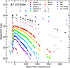 |
Fig. 1. Optical, NIR, and MIR light curves of AT 2019abn. The filled circles represent the unpublished data, while the empty circles represent the data points from the literature. The empty triangles represent the upper limits. |
3.2. AT 2019ahd
The discovery of AT 2019ahd was reported by the ATLAS survey (Tonry et al. 2019; Smith et al. 2020) on 2019 January 29.0 UT. The coordinate of the transient are RA = 10h51m11s.737 Dec = +05° 50′ 31 03, which is 2
 6 north and 6
 9 south of the centre of its host, the spiral galaxy NGC 3423. As the distance modulus of the host galaxy, we chose to adopt an average of the different independent values reported on the NASA/IPAC Extra-galactic Database (NED, Helou et al. 1991) obtaining a distance modulus μ = 30.22 ± 0.14 mag, where the error comes from the standard deviation of the measurements (Tully & Fisher 1988; Tully et al. 1992, 2009; Nasonova et al. 2011). We assumed a cosmology where H0 = 73 km s−1 Mpc−1, ΩΛ = 0.73 and ΩM = 0.27 (Spergel et al. 2007), which will be used throughout this whole work. The Galactic absorption in the direction of NGC 3423 is AV = 0.079 ± 0.003 mag (Schlafly & Finkbeiner 2011). The object was initially classified as a Luminous Blue Variable (LBV, Jha 2019) due to its narrow hydrogen features and relatively red spectrum. The following photometric and spectroscopic evolution of the transient, in particular the prevalence of calcium features (Ca II H&K, [Ca II] and Ca NIR triplet; see Paper II), proved that it is an ILRT instead. The majority of the follow-up performed for this object was obtained with the GROND instrument mounted at the 2.2m telescope at ESO’s La Silla observatory, which yielded a remarkably homogeneous dataset (Figure 2). The brightest magnitude is well constrained at mr = 17.57 ± 0.07 mag, reached on MJD = 58525.0. Similar to AT 2019abn, AT 2019ahd displays a slow decline just after peak luminosity (γ1 = 1.12 ± 0.09), but this pseudo-plateau only lasts for 45 days, followed by a steeper decline (γ2 = 2.31 ± 0.10) that ends 105 days after maximum. The subsequent decline rate is again slower (γ3 = 1.05 ± 0.03), in particular in the NIR bands.
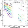 |
Fig. 2. Optical and NIR light curves of AT 2019ahd. Filled circles represent unpublished data, while empty circles represent ZTF data points. Empty triangles represent upper magnitude limits. Magnitude shifts on i and z bands have been applied for clarity. |
3.3. AT 2019udc
The discovery of AT 2019udc was reported by the ‘Distance Less Than 40 Mpc survey’ (DLT40, Tartaglia et al. 2018) on 2019 November 4.1 UT. The transient lies on a spiral arm of the galaxy NGC 0718, at RA = 01h53m11s.190 Dec = +04°11′ 46 96. We adopted a kinematic measure of distance for NGC 0718, which provides μ = 31.49 ± 0.15 mag, obtained through the redshift of the galaxy with respect to 3K CMB (Fixsen et al. 1996). The Galactic absorption towards NGC 0718 is AV = 0.100 ± 0.001 mag. Similar to AT 2019ahd, also AT 2019udc was originally classified as an LBV due to its spectral features (Siebert et al. 2019) but its evolution proves that it is actually an ILRT. AT 2019udc is the most distant object studied in this sample. The follow-up campaign was suspended 120 days after maximum, due to solar conjunction. The GSP multi-band monitoring yielded a high-cadence follow-up of the rise and peak of AT 2019udc, crucially contributing to the collection of a high-quality dataset for this object (Figure 3, left panel). During the first two days after discovery (−10 to −8 days from maximum), the rise in magnitudes can be approximated as linear, with an increase rate up to three time faster than the rise of AT 2019abn, with bluer bands showing a systematically faster evolution (γ1 = −47.5 ± 4.8). After this phase the rise quickly slows down, departing from a linear behaviour and reaching peak luminosity in about 10 days (mr = 17.40 ± 0.06, MJD = 58801.28). Immediately after maximum, AT 2019udc displays a fast linear decline (γ2 = 3.93 ± 0.09), again around three times faster than the decline of AT 2019abn just after maximum. The luminosity drop settles on a gentler slope in all bands at around 35 days after maximum (γ3 = 2.22 ± 0.12). The resulting light curve is noticeably fast evolving for an ILRT: although peculiar compared to the other objects in the sample, these features are not unique among ILRTs, as shown in Sect. 7.
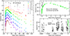 |
Fig. 3. Photometric data collected for AT 2019udc. In the right panel we present optical and NIR light curves of AT 2019udc. Magnitude shifts have been applied for clarity. Filled circles represent unpublished data, while empty circles represent ZTF data points. In the left panels is shown DLT40 monitoring of AT 2019udc. In particular, in the upper left panel is shown the high-cadence follow-up of the rise of AT 2019udc. The DLT40 data points are shown as stars and are integrated with observations obtained through other facilities, represented as circles. In the lower left, years of upper limits collected by DLT40 are displayed as black triangles, with the detections of the transient appearing as green symbols at the right edge of the figure. |
Thanks to the prompt discovery and high-cadence monitoring of the DLT40 survey, the luminosity rise of AT 2019udc is exceptionally well sampled, as presented in the upper right panel of Figure 3 (DLT40 data are unfiltered observations scaled to sloan r band observations). The rise immediately after the discovery is remarkably fast, 0.8 magnitudes in less than one day, followed by a more gentle brightening of 0.6 mag in 2.5 days. At this point, 3 days after the first DLT40 detection, AT 2019udc is already close to maximum luminosity, and its magnitude will only marginally change (within ±0.15 mag) in the following two weeks We tried to fit the rise to maximum of AT 2019udc with a simple fireball model, where the flux increases as t2 (as detailed by e.g. Nugent et al. 2011). However, as shown by the black solid line in the upper right panel of Figure 3, the observed light curve quickly departs from the fireball model extrapolated from steep rise of the first two days. One possible explanation for this discrepancy is that the early light curves of ILRTs are not dominated by 56Ni decay, unlike the light curves of SNe Ia (for which the fireball model is a reasonable approximation). DLT40 also provides several years of upper limits to the optical luminosity of the progenitor of AT 2019udc, which are displayed in the lower right panel of Figure 3. The absence of outbursts and the overall non-detection in the optical domain of the progenitor of AT 2019udc is well in line with the expectations for ILRTs, whose precursors have been identified as dust enshrouded stars, heavily affected by extinction in the optical wavelengths but luminous in the MIR (Thompson et al. 2009).
3.4. NGC 300 2008 OT-1
NGC 300 2008 OT-1 (hereafter NGC 300 OT) was discovered on 2008 May 14 during the SN search program at the Bronberg Observatory (Monard 2008). The event, located in the nearby NGC 300 at RA = 00h54m34s.51 Dec = −37° 38′ 31 4, was extensively studied in the subsequent years (Bond et al. 2009; Berger et al. 2009; Humphreys et al. 2011; Adams et al. 2016) and became a prototype for the class of ILRTs together with SN 2008S (Botticella et al. 2009). Here we present additional optical, NIR and MIR data, adding this object to our sample of ILRTs. For the distance of NGC 300, we adopted the results published by Gogarten et al. (2010), where a distance modulus μ = 26.43 ± 0.09 mag is obtained through the red clump method. The Galactic absorption towards NGC 300 is AV = 0.034 ± 0.001 mag (Schlafly & Finkbeiner 2011). NGC 300 OT is the closest ILRT ever observed, making it an extremely valuable target which was monitored in detail for an extended period of time. In Figure 4 we present the original optical and NIR photometric data we collected for this transient. The object was behind the sun during its rise and peak luminosity, so we lack the first part of its evolution. Our observed maximum is mr = 14.38 ± 0.02 mag on MJD = 54602.38. We note that there is a serendipitous optical detection of NGC 300 OT on MJD = 54580.65 when the transient is rising (mR = 16.30 ± 0.04 mag, Humphreys et al. 2011), providing a rough estimate for the onset epoch of the event. The first 35 days display a slow decline (γ1 = 1.11 ± 0.05), especially in the red bands. From 35 to 75 days, the transient falls from this pseudo-plateau, and its luminosity starts to fade faster (γ2 = 3.32 ± 0.08). Between 75 and 120 days the decline in luminosity is particularly rapid (γ3 = 5.24 ± 0.06, calculated on the R band due to lack of r band coverage in this phase), comparable to the fast declining phase of AT 2019udc. From 120 and 255 days the fast decline stops, and a slow evolution ensues (γ4 = 0.69 ± 0.07) before the final phase (γ5 = 1.56 ± 0.05) that encompasses from 255 days onwards. As done for AT 2019abn, we integrated the dataset provided by Humphreys et al. (2011) with our observations by applying magnitude corrections to their observations, calculated by measuring the magnitude of the reference star chosen in their work: ΔB = +0.07 mag, ΔR = +0.05 mag. No correction was needed for V band, I band and NIR data, since they were perfectly matching. We also performed aperture photometry on the public images of NGC 300 OT taken with Swift Ultraviolet and Optical Telescope (UVOT), which were also analysed by Berger et al. (2009). We find a remarkable agreement in the U, B, V magnitudes reported there, while we measure overall fainter UVW2 and UVW1 magnitudes, possibly due to a different background selection: in particular, we restricted the aperture down to 3″ to limit possible background contamination. The resulting UV fluxes from our measurements are in line with the behaviour expected from a blackbody emission, as shown in the top left panel of Figure 7.
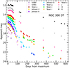 |
Fig. 4. UV, optical, and NIR light curves of NGC 300 OT. Empty triangles represent upper limits. Filled circles represent unpublished data, while empty circles represent publicly available SWIFT data. |
3.5. Comparison with other transients
In Figure 5, we compare the absolute r and H band evolution of our sample of ILRTs along with that of other transients of similar luminosity. The first considerations can be made observing the sample of ILRTs, with the addition of the well studied SN 2008S (Botticella et al. 2009) and AT 2017be (Cai et al. 2018). We note the large spread in the optical peak magnitudes, which spans from −12 mag for AT 2017be to almost −15 mag for AT 2019abn. We note that AT 2019abn (Mr = −14.66 ± 0.15 at maximum) is, to date, the brightest ILRT ever observed, with AT 2019udc (Mr = −14.17 ± 0.16 at maximum) also falling on the brighter end of the ILRTs luminosity distribution. AT 2019ahd and NGC 300 OT, instead, display fainter peak magnitudes, −13.00 ± 0.16 mag and −12.91 ± 0.14 mag respectively. Among the least luminous ILRT we find AT 2017be, which is barely brighter than Mr = −12 mag. There are also significant differences in light curve shapes within the class. AT 2019abn and AT 2019udc represent the two extreme cases, with the former being characterised by a long phase of slow decline after peak, almost a pseudo-plateau in the r band (1.37 ± 0.01 mag/100 days), while AT 2019udc undergoes a decline that is three times faster (3.93 ± 0.09 mag/100 days), after peak luminosity. This variability is less pronounced in the NIR domain, where both the decline rates and the peak magnitudes span a smaller range of values. Regardless of their differences, ILRTs tend to settle on a linear decline at late times, which is compatible with the expected luminosity decline sustained by 56Ni radioactive decay. This can be visually evaluated by comparing the late-time behaviour of ILRTs with that of SN 2005cs, one of the prototypes of low-luminosity SNe IIP (Pastorello et al. 2009), whose late decline is known to be powered by 56Ni decay. We also note that SN 2005cs is fainter than AT 2019abn at peak luminosity, revealing an overlap between the brightest ILRTs and the faintest core collapse SNe. To summarise the features described above, ILRTs are characterised by their single-peaked, monotonically declining light curves which terminate in a linear decline at late phases. A clearly different light curve shape is instead associated with luminous red novae (LRNe, Pastorello et al. 2019b), another class of transients populating the luminosity ‘gap’ which separates classical novae from standard SNe. LRNe are non-degenerate stellar mergers, and typically display double peaked light curves, as shown for by AT 2017jfs (Pastorello et al. 2019a) and to a lesser degree M31-LRN-2015 (Williams et al. 2015), both reported in Figure 5. With its peak absolute magnitude fainter than –10 mag, M31-LRN-2015 appears detached from the other transients shown: LRNe can be much dimmer, with peak absolute magnitude even below ∼–4 mag (e.g. V1309Sco Tylenda et al. 2011). On the other hand, the ILRTs discovered to date have been strictly confined within the luminosity gap (−10 mag < MV < −15 mag).
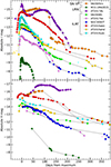 |
Fig. 5. Absolute r band (upper panel) and H band (lower panel) light curve comparison between the ILRTs in our sample and other low-luminosity transients. In particular, ILRTs are marked with circles, LRNe with plus signs, and SN IIP with diamonds. |
4. Reddening estimate
Estimating the reddening affecting ILRTs is a challenging task, and different approaches can be found in the literature, depending on the available data. A first method consists in using the empirical relation between the Na ID Equivalent Width (EW) and the absorption along the line of sight (Turatto et al. 2003; Poznanski et al. 2012), as was done by Cai et al. (2018). This method has the advantage of not requiring any assumption on the intrinsic properties of the target, but it needs high S/N spectroscopy in order to be reliable. Furthermore, the EW of Na ID observed may saturate, preventing the application of empirical relations (e.g. Stritzinger et al. 2020). In addition to this, the EW of the Na ID varies with time in ILRTs (e.g. Byrne et al. 2023, and further discussed in Paper II), increasing the uncertainty associated with this method. Finally, as pointed out by Poznanski et al. (2012), if the extinction towards a target is dominated by circumstellar dust, this empirical relation between the Na ID EW and reddening might be unreliable. A second method is based on the observation that the spectral features of ILRTs resemble those of F-type stars (Humphreys et al. 2011; Jencson et al. 2019). It is then assumed that all ILRTs reach a temperature of ∼7500 K at maximum luminosity, and a reddening correction is applied to the SED at peak in order to obtain a blackbody continuum corresponding to such temperature. Yet another strategy is adopted for SN 2008S by Botticella et al. (2009), who estimate the extinction affecting the target based on an IR echo model of the SED at early stages. Notably, different methods have been adopted in different studies of NGC 300 OT, even reaching opposite conclusions: Berger et al. (2009) deem the reddening along the line of sight to be minimal based on the measurement of the Na ID EW, while the DUSTY models discussed by Kochanek (2011) envision important extinction, leading a peak as high as 9000 K. This heavy dust extinction inferred is quite dependent on the extrapolation of the MIR contribution at early phases (e.g. Figures 5 and 7 in Kochanek 2011).
In this work we adopted the same procedure carried out by Stritzinger et al. (2020), who noted that the observed V–r and r–i colour curves of several ILRTs have a similar shape. Assuming that ILRTs should display a similar evolution of optical colours, a reddening estimate can be obtained by attempting to match the colour evolution of the bluest objects. While this is likely an approximation, it is not baseless, since these transients present a marked homogeneity in their optical spectra (which will be further discussed in Paper II): since similar conditions in temperature and ionisation state are required to produce the same spectral features, we can expect the optical colours of these transients to be at least compatible in their photospheric phases. Following this reasoning, we considered the bluest object in our sample, AT 2019udc, together with AT 2017be, which shows remarkably similar colours, and we applied a reddening correction to all the other objects in our sample in order to superimpose their B − V, g − r and r − i colour curves through a least squares minimisation procedure. Only the values measured within 40 days after maximum are considered. The absorption values for each transient inferred in this way are reported in the last column of Table 1. AT 2019abn is by far the most reddened object in our sample, with an estimated internal absorption of AV = 1.84 ± 0.20 mag. AT 2019udc, by construction, is assumed to be reddening-free, since it is among the bluest ILRT observed. We note that the errors reported on the extinction values are just the errors linked to the least squares minimisation procedure: these will be the values adopted in the following analysis as our best estimates, but there are sources of systematic uncertainty which are challenging to account for. Notably, it is reasonable to expect some scatter in the temperature and consequently in the colours of ILRTs, also due to possible surviving dust affecting the transient. However, all of them should fulfil the physical requirements for producing the H and Ca II lines observed in their spectra (discussed more in detail in Paper II). Ca II spectral features appear in type II SNe only when the temperature of the photosphere has dropped below ∼10 000 K (e.g. see the evolution of SN 2005cs, Pastorello et al. 2006): this can be treated as an upper limit to the peak temperature of ILRTs, since Ca II features are found in their spectra at all phases. On the other hand, given the strong Balmer lines that dominate their spectra, it is reasonable to infer that the hydrogen was ionised by the event, suggesting that after reddening correction the maximum temperature should not be below ∼5500 K, a typical value adopted for hydrogen recombination temperature (Branch & Wheeler 2017). This range of temperatures (and therefore of possible extinction values) is quite broad, but we note that our choice of reddening is corroborated by the Balmer decrement observed for our sample of ILRTs, which is close to 3 during the early phases (see Figure 4 in Paper II). This is indeed the value expected for the case B recombination of hydrogen (Osterbrock & Ferland 2006), supporting the idea that the absorption estimated is a valuable first order correction. In Figure 6 we report the colour evolution for our sample of ILRTs after applying the reddening correction. The optical colours present an initial decrease (i.e. the objects become bluer) during the rise to maximum. This is particularly clear in AT 2019udc and AT 2019abn, thanks to their high-cadence monitoring pre-maximum. After peak luminosity, ILRTs become steadily more red in the following months. This trend may invert as the flux becomes dominated by emission lines rather than continuum emission, as seen for NGC 300 OT r − i after 150 days post maximum. We note that we are using a conservative estimate for the reddening affecting SN 2008S, for which we adopt just the Milky Way absorption of AV = 1.13 mag. This is a lower limit to the total reddening along the line of sight: adopting a light echo model, Botticella et al. (2009) infer an internal absorption of AV ∼ 1 mag, which leads to a peak temperature of 8400 ± 120 K. In any case, even with minimal absorption, SN 2008S is among the bluest ILRTs to date.
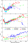 |
Fig. 6. Colour curves after reddening correction for the ILRTs belonging to our sample, with the addition of SN 2008S and AT 2017be. In the top two panels the optical colours are shown, in the bottom panel the NIR colour evolution. |
Key information regarding the transients in the sample.
For the sake of completeness we compare the reddening estimates just obtained with a straightforward application of the linear relations between Na ID EW and E(B − V) presented by Turatto et al. (2003). The detailed evolution of the Na ID EW for this sample of ILRTs will be shown and discussed in Paper II: here we simply consider the first measured value for each transient, specifically 0.7 ± 0.1 Å for NGC 300 OT, 1.1 ± 0.1 Å for AT 2019abn, 0.9 ± 0.1 Å for AT 2019ahd and 5.4 ± 0.2 Å for AT 2019udc. The two different linear relations provided by Turatto et al. (2003) allow to determine both a lower and upper estimates of E(B − V) for each object. The resulting AV range obtained for NGC 300 OT spans between 0.3 and 0.9 mag, compatible with our previous estimation of 0.94 mag. In case of the lowest reddening inferred, the peak luminosity of NGC 300 OT in r band would be 0.6 mag fainter, leading to a peak absolute magnitude Mr = −12.3 mag. For AT 2019ahd we obtain 0.4 mag < AV < 1.3 mag, with the lower limit being compatible with our previous measurement of 0.31 mag. If we accept the larger estimate of AV ∼ 1.3 mag, the peak r band absolute magnitude of AT 2019ahd would increase from −13.0 mag to −13.9 mag. For the other two ILRTs in the samples the two methods for estimating AV yield more substantial differences. According to the empirical relations obtained by Turatto et al. (2003), the EW of the Na ID observed in the early phases of AT 2019abn would imply an extinction of 0.5 mag < AV < 1.6 mag, significantly lower than the value 1.84 mag previously obtained. The peak absolute magnitude of AT 2019abn would decrease from Mr = −14.7 mag to −14.4 mag, or even −13.5 mag in the case of lowest extinction. On the contrary, AT 2019udc initially displays a remarkably large Na ID EW of 5.4 ± 0.2 Å (however, we note that the Na ID EW rapidly declines to 1.3 Å in just two days, and even below 1 Å after that phase): this would imply an extinction AV of at least 2.6 mag. The resulting peak magnitude would be at least Mr = −16.5 mag, firmly within the luminosity realm of full-fledged SNe. These critical discrepancies in AV would also lead remarkable variations in temperature, in particular AT 2019abn would present a peak temperature even below that of hydrogen recombination, while AT 2019udc could reach temperatures high enough to inhibit the formation of Ca II lines. This is an unlikely circumstance, given the already mentioned spectral homogeneity of ILRTs.
5. SED evolution
In order to extract physical quantities of our targets, we performed blackbody fits on the SED at different epochs. This analysis was carried out through Monte Carlo simulations, using the PYTHON tool CURVE_FIT5 to perform fits on 200 sets of fluxes randomly generated with a Gaussian distribution centred at the measured flux value, and σ equal to the error associated with the measurement. This procedure was already adopted and described in Pastorello et al. (2021), Valerin et al. (2022). The blackbody fit to the SED of the target yielded the estimated temperature, and by integrating over the wavelength we obtained the total flux emitted. Adopting the distances discussed in Sect. 3 and assuming spherical symmetry, we calculated the bolometric luminosity of the source. Finally, the radius was estimated through the Stefan–Boltzmann law. This whole procedure was repeated for each epoch with suitable photometric coverage, in order to study the evolution of the inferred physical parameters with time. During their first evolutionary phase all our objects are well fit by a single blackbody, associated with the photosphere, throughout the optical and NIR domains (Figure 7). We refer to this component as the hot blackbody, in contrast with the cold blackbody that emerges at later stages. A notable exception is AT 2019abn, which shows a NIR excess compared to a single blackbody from the very first epoch in which NIR data are available (upper left panel of Figure 7). This can be interpreted as the emission from pre-existing dust that survived the explosion, as observed for SN 2008S (Botticella et al. 2009). This NIR excess disappears quickly within a few days, and MIR observations confirm that the flux in the optical domain dominates the SED of AT 2019abn for months after peak luminosity, only requiring a single blackbody to be reproduced. The phase in which a single blackbody is sufficient to model the SED has a variable duration in each transient: up to 180 days for AT 2019abn, 110 days for AT 2019ahd and only 80 days for NGC 300 OT. The SED of AT 2019udc is well fit by a single blackbody during our monitoring before solar conjunction, roughly 100 days after peak luminosity. After solar conjunction, the object was below the detection threshold in the optical domain, but it was still visible in NIR images, showing a SED compatible with a relatively cool blackbody. In other words, in AT 2019udc we likely missed the transitional phase in which both the hot and the cold blackbodies are visible at the same time due to solar conjunction.
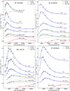 |
Fig. 7. SED evolution of AT 2019abn, AT 2019ahd, NGC 300 OT, and AT 2019udc. Flux measurements are shown as black circles. In the first phases of their evolution, a single blackbody closely approximates the evolution of the SED. At later phases a second cooler blackbody is needed to reproduce the NIR flux excess. Epochs are reported with respect to maximum light. Flux shifts have been applied for clarity. |
The values of temperature, luminosity and radius obtained for this hot blackbody are displayed in Figure 8. The temperature evolution of our sample is especially homogeneous between 25 and 75 days after maximum, due to our reddening estimate through colour curves superposition (Sect. 4). However we still find interesting differences between the various targets in the pre-maximum phases. AT 2019abn displays an almost constant temperature of ∼4300 K for several days before slowly reaching the peak temperature of ∼5300 K in ∼20 days. AT 2019udc qualitatively follows the same behaviour, but in a shorter timescale (less than 10 days) and reaching 7000 K at peak. This initial increase in temperature could be explained with the injection of additional energy provided by the interaction between ejecta and circumstellar medium (CSM), as happens for interacting SNe (e.g. Dessart et al. 2016). AT 2019ahd, on the other hand, starts from a temperature of ∼7100 K, before quickly cooling to 5900 K at peak luminosity. From this point onwards, AT 2019ahd closely follows the behaviour of AT 2019abn. In this respect, the early temperature evolution of AT 2019ahd is reminiscent of that of SN 2005cs (displayed in Figure 8 for comparison) and LL SN IIP in general, where the temperature quickly declines during the rapid expansion of the ejecta. NGC 300 OT shows a very simple, monotonic temperature evolution, but in this case we miss the pre-maximum photometric coverage.
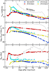 |
Fig. 8. Temperature, luminosity, and radius evolution of the hot blackbody of the four ILRTs in our sample. The same values measured for SN 2005cs are shown as a dotted line for comparison. |
In the middle panel of Figure 8 we present the bolometric luminosity obtained for the “hot” blackbody. The bolometric luminosity behaves in a similar way to what is described in Sect 3.5, with AT 2019abn and AT 2019udc reaching a similar peak luminosity of 1.4 × 1041 erg s−1. As previously pointed out, their decline rate is quite different: AT 2019udc is characterised by a marked peak followed by a fast decline, while the evolution of AT 2019abn is slower compared to other objects of the same class, although not as flat as the plateau of SNe IIP. AT 2019ahd and NGC 300 OT display more modest peak luminosities, respectively of 4.1 ± 1.0 and 3.4 ± 1.0 × 1040 erg s−1. As for the evolution of the radius of the emitting source, shown in the bottom panel of Figure 8, it appears that all ILRTs in our sample follow a similar behaviour. After maximum, the transients show a roughly constant radius with time, although with different values. AT 2019abn again stands out from the group, showing a blackbody radius that at first quickly increases from 18 ± 2 to 36 ± 3 AU from discovery to peak luminosity, and then remains at 30 to 40 AU in the following 125 days. These values are roughly two to three times those obtained for the other three targets. AT 2019ahd shows qualitatively the same behaviour, with a radius growing from 7 ± 1 to 15 ± 1 AU from discovery to peak magnitude, and a subsequent slow evolution ranging from 14 ± 1 to 18 ± 1 AU within 110 days after maximum. AT 2019udc on the other hand does not show an increase in the radius during the pre-maximum phase, but rather a marginal decrease, from 23 ± 3 to 19 ± 2 AU. The following slow evolution of the blackbody radius between 16 ± 2 and 21 ± 2 AU over the course of 90 days is reminiscent of those of the other two ILRTs already presented. Finally, for NGC 300 OT we do not have pre-maximum data, but the evolution of the blackbody radius after the observed maximum is again slow, spanning from 16 ± 1 to 11 ± 1 AU in 90 days. This tendency of the hot blackbody radius to linger around a constant value is in stark contrast with the monotonic increase in radius for SNe IIP and LL SNe IIP during the first 80 days, as shown by the radial evolution of SN 2005cs.
So far we described the physical properties of the hot blackbody, which is associated with the photosphere of the transient and is usually well visible for ∼100–150 days after maximum. At later phases however, as the gas cools down and expands, an excess in the NIR flux is detected (extending to the MIR, when such measures are available). This feature can be associated with the formation of dust, which contributes to the SED with a second emission component characterised by a low temperature compared to the hot continuum observed in the first months of evolution (T ≲ 1500 K, Botticella et al. 2009; Cai et al. 2018). In Figure 7 are shown the blackbody fits performed to the SED of our targets at epochs when two components coexist. At the latest phases, as the objects shift from the photospheric to the nebular phase, the optical flux is entirely supported by emission lines (Hα, Hβ, [CaII], Ca NIR triplet), and there is no more evidence of a hot spectral continuum. At these epochs we still identify a contribution from the cold blackbody associated with dust emission. This feature is especially clear in AT 2019abn and NGC 300 OT (at 761 days after maximum, see Sect. 6.1) thanks to the MIR measurements. In Figure 9 we present the physical parameters obtained for the cold blackbody component associated with dust emission. In principle this cold blackbody could be the result of a NIR light echo (e.g. Miller et al. 2010). However, the timing of the appearance of this NIR excess (80 days for NGC 300 OT being the shortest) would imply that the dust causing the light echo is located at least ∼6900 AU away from the transient. Botticella et al. (2009) show that the flash from SN 2008S is able to create a dust-free cavity of just ∼2000 AU: it appears unlikely that the energy radiated by our ILRTs can bring such a distant body of dust close to its sublimation temperature (∼1400 K for silicates and ∼1800 K for graphite; e.g. Jiang et al. 2016). Therefore, we favour the interpretation that this cold blackbody component is emitted by newly condensed dust rather than by a light echo. As mentioned above, AT 2019abn displays a NIR excess that can be associated with dust emission even during its rise to maximum. The cold blackbodies resulting from the fit of the NIR excess have a luminosity of 1.3 ± 0.5 × 1040 erg s−1, with temperature decreasing from 1750 K to 1500 K and radius increasing from 90 to 130 AU in one day. After the second detection, at −17 days with respect to maximum, the NIR excess quickly fades, possibly dominated by the increasing contribution from the photosphere of the transient. The cold component reappears in AT 2019abn at ∼180 days, diminishing both in luminosity (from 5 to 2 × 1039 erg s−1) and in temperature (from 1700 K to 1200 K) over the course of about 240 days. After an initial decrease to 45 AU, the radius of the cold blackbody remains around 75 AU. AT 2019ahd develops the cold component sooner, around 110 days. At this phase, the luminosity of the cold blackbody component is ∼3.8 × 1039 erg s−1, with temperature ∼1400 K and radius of ∼80 AU. We stress that the blackbody fits in the earlier epochs are affected by large errors, due to the uncertainty in disentangling the hot and cold components in the SED. At later phases, the behaviour of the cold component of AT 2019ahd is remarkably similar to the one already described for AT 2019abn. For AT 2019udc we have a single late-time observation with coeval J, H and K observations which allows us to perform a credible blackbody fit: the parameters inferred for the dust in AT 2019udc are well in line with those measured at a similar phase for AT 2019ahd and AT 2019abn, in particular a temperature of 1500 ± 100 K, a luminosity of 3.8 ± 0.8 × 1039 erg s−1 and a radius of 68 ± 9 AU.
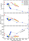 |
Fig. 9. Temperature, luminosity, and radius evolution of the cold blackbody of the ILRTs in our sample. In the third panel, the dashed line represents the position of material expanding with velocity of 550 km s−1. |
In the case of NGC 300 OT, we have a higher cadence of NIR observations (also accounting for previously published observations), allowing us to better constrain the evolution of the cold component. A first, we observe a rather constant temperature ∼1500 K between 70 days and 130 days after maximum. During this time the luminosity of the cold component decreases from 4.8 to 2.6 × 1039 erg s−1, with a consequent shrinkage of the radius from 80 to 60 AU. At this point, the temperature quickly drops to ∼1000 K over the course of 70 days, with the luminosity slowly increasing to 3.6 × 1039 erg s−1 as the radius increases to 150 AU. The subsequent temperature decline is slower, reaching 590 ± 5 K at 761 days, when the transient has faded to 9.3 ± 1.5 × 1038 erg s−1. In the time between 400 days and 760 days the radius slowly increases from 120 AU to 220 AU. This late estimate is possible thanks to publicly available WISE data discussed in the Sect. 6.1. The other two late measurements at 398 and 582 days were performed on MIR data taken by Ohsawa et al. (2010). The bimodal trend for the blackbody radius evolution, which shows an initial shrinking followed by an expansion, has also been discussed by Kochanek (2011) and can be explained as follows. At first we are observing dust formation far from the ejected material, with dust condensing at progressively smaller radii as the transient becomes dimmer and the temperature decreases. We know that the progenitor star was enshrouded in dust (Thompson et al. 2009) before the transient event caused its sublimation, and we may be witnessing the rebirth of this dusty cocoon. As the inner boundary of the condensing dust is reached by the ejected material (or the shock induced by the ejected material in the CSM), the radius of emitting dust starts to increase. This behaviour is also found in SNe, where the dust expands together with the ejecta (e.g. Wesson et al. 2015). As a simple comparison, in the bottom panel of Figure 9 we mark with a dashed line the position of matter expanding with a velocity of 550 km s−1, and we note that the three latest radius measures for NGC 300 OT are compatible with this trend. As will be shown in Paper II, the velocity of 550 km s−1 is also well in line with the full width at half maximum velocity estimated from the emission lines of NGC 300 OT, corroborating the idea that the dust is moving jointly with the expanding gas seen during the photospheric phase. This velocity is also in line with the shock velocity of 560 km s−1 adopted for NGC 300 OT by Kochanek (2011). In this context, it could be tempting to interpret the faster radius increase observed between 130 and 200 days as an indicator of faster material, moving at ∼1200 km s−1. However, the lack of MIR coverage in this critical phase may be noteworthy, as we have to rely on extrapolations based on J, H and K bands for a source rapidly cooling to ∼1000 K. In the latest three epochs, instead, the SED is firmly constrained in the NIR and MIR domains, leading to robust estimates.
The qualitative behaviour of the dust described above is in agreement with the interpretation provided by Kochanek (2011); however, we note that in their analysis both the luminosity and the emitting radius of the dust during the first months of evolution of NGC 300 OT are remarkably higher compared to the results obtained in this section. Kochanek (2011) models the SED of NGC 300 OT through the radiation transfer code DUSTY, which incorporates larger reddening values compared to the ones we adopted, resulting in a larger contribution from the hot blackbody component. Furthermore, the model presented by Kochanek (2011) envisions a significant flux contribution in the MIR domain even during the first three months of evolution, a period during which there are no confirmed MIR detection available (see the first panels of their Figure 5 and Figure 7). Compared to this model, our extrapolation through a blackbody leads to a more modest luminosity contribution in the MIR domain for NGC 300 OT. Such an important increase in flux in the model by Kochanek (2011) is accompanied by larger estimate of the dust radius, which is the first phases is up to ∼100 times larger than what we inferred in our analysis. However, we note that this tension dissipates at later phases, especially when considering late-time observations when MIR data are available: for example, at 761 days after maximum, our estimate of the dust radius of NGC 300 OT is compatible within their error bars with the value provided by Kochanek (2011). This highlights the importance of MIR observations for ILRTs throughout their whole evolution, because unlike other transients the luminosity contribution from this domain could be relevant even at early phases. In any case, the MIR data collected for AT 2019abn show that a remarkable MIR contribution to the SED during the photospheric phase is not ubiquitous in ILRTs (Figure 7).
In order to obtain the bolometric luminosity of ILRTs, we combined the contribution of the hot, photospheric component, and the cold, dusty component. At late epochs, a blackbody continuum is no longer discernible in the optical domain, with only emission lines dominating the spectra. Therefore, to measure the bolometric luminosity in those cases we integrated the fluxes in the optical domain using the trapezoidal rule. On the other hand, at longer wavelengths it was still possible to perform a blackbody fit and integrate the flux even beyond the observed spectral region. While the optical domain only displays emission lines at late times, there still is still evidence of thermal continuum in the NIR and MIR domain. The bolometric luminosity obtained for our sample of ILRTs is reported in Figure 10. We analysed an unprecedented amount of NIR and MIR data for ILRTs, which allowed us to better infer the luminosity contribution at longer wavelengths, crucial at late times. The dotted lines in Figure 10 show the expected behaviour of a light curve powered exclusively by 56Co decay: it is evident that AT 2019abn, AT 2019ahd, and NGC 300 OT are characterised by a late-time decline shallower than what is expected if only 56Co decay is supporting their late-time luminosity. We note that a more shallow slope in the light curve does not exclude the presence of 56Co, but rather requires an additional mechanism to explain the late-time luminosity of ILRTs. Kochanek (2011) suggests that the late-time luminosity of NGC 300 OT is powered by the shocks propagating within the dusty progenitor wind, which produce X-rays that are promptly thermalised and re-emitted as optical and infrared radiation. This explanation could be valid also for AT 2019abn, given the dusty nature of its progenitor star (Jencson et al. 2019), and it can be further extended to AT 2019ahd. In order to estimate an upper limit to the 56Ni mass powering the late linear decline of ILRTs, we employed the analytical formulation provided by Hamuy (2003) for the luminosity of 56Ni and 56Co decay. Considering the first data points available during each linear decline, we obtained upper limits to the 56Ni mass of 5.9 × 10⁻³ M⊙ for AT 2019abn, 2.0 × 10⁻³ M⊙ for AT 2019ahd, and 1.1 × 10⁻³ M⊙ for NGC 300 OT. AT 2019udc is the only object that shows a linear decline fully compatible with the one expected from 56Co decay, resulting in an estimate of 3.3 ± 0.3 × 10⁻³ M⊙ of 56Ni.
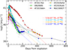 |
Fig. 10. Bolometric light curves of our sample of ILRTs, together with SN 2008S and AT 2017be. The coloured dotted lines show the 56Ni decline rates for the upper limits estimated for each object in oursample. |
We can also provide values of the total energy radiated by our ILRTs during the time they were monitored: NGC 300 OT emitted 2.7 × 1047 erg over the course of 760 days, with 1.8 × 1047 erg released in the first 120 days after maximum. Similarly, AT 2019ahd radiated 3.8 × 1047 erg in 440 days, 2.2 × 1047 erg in the first 100 days, while AT 2019udc emitted 4.0 × 1047 erg in about 100 days. Finally, AT 2019abn radiated 1.3 × 1048 erg in 480 days, the vast majority (1.2 × 1047 erg) emitted in the first 240 days. Aside from the total energy released by these transients, the decline rate of their bolometric luminosity at late time appears particularly interesting.
6. Late-time MIR monitoring of ILRTs
6.1. Dust evolution and composition
Ohsawa et al. (2010) monitored the evolution of NGC 300 OT in the IR domain (2–5 μm) at 398 and 582 days, finding that the hot dust component had progressively cooled down to 810 K and ultimately to 680 K. The probed wavelength range did not provide information on the cool, pre-existing dust component, which by that time could only contribute ∼1% of the observed flux. Ohsawa et al. (2010) also set lower limits for the optical depth of the dust: τν > 12 at 398 days and τν > 6 at 582 days, effectively stating that the dust remains optically thick even at very late phases. In this condition, the lower limit to the mass of emitting dust was estimated to be ∼10−5 M⊙.
Thanks to the WISE data collected on 2010 June 17 in the W1, W2, W3, and W4 filters, we were able to expand the analysis on the late-time evolution of the dust in NGC 300 OT, 761 days after maximum. To correct these values for absorption, we extended the reddening law to 22 μm by employing the tabulated values and prescriptions found in Rieke & Lebofsky (1985) and Draine (1989). The late-time K band coverage with SOFI obtained 853 days after maximum allowed us to linearly extrapolate the K-band flux at 761 days in order to have a more detailed SED of the transient. We fit our flux measures through the same procedure detailed in Sect. 5. Following in the footsteps of Ohsawa et al. (2010), instead of a simple Planck function we used f(ν)∝(1 − e−τν)Bv(Td) as a fitting function, where τν is the optical depth, Bν is the Planck function and Td is the dust temperature. The multiplicative factor in front of the Planck function aims to account for the different opacity of dust at different wavelengths. It is relevant to point out that this model is isothermal, while a cloud of optically thick dust would present a temperature gradient, so this is already an approximation.
To better differentiate the properties of the dust depending on the size of the dust grains and their chemical composition, we performed the fits using four different sets of opacity kν, tabulated by Fox et al. (2010). Two sets are opacity values for graphite dust, with grain size of 0.1 and 1 μm respectively, while the other two sets of opacity assume the same grain size, but present a silicate composition. Since the values presented by Fox et al. (2010) only cover up to 13 μm while our data reach 22 μm (thanks to the W4 channel), we had to extrapolate the behaviour of kν in that region. For the graphite dust we followed the prescription from Draine (2016), using a λ−2 scaling. The silicate opacity is instead characterised by an additional bump in opacity around 19 μm: to reproduce it, we adopted the opacity behaviour reported by Draine & Lee (1984). Beyond 9 μm, graphite dust tends to have a lower opacity compared to graphite dust (see Figure A.1). Silicate dust stands out because of the ‘bumps’ in opacity in the MIR domain, in contrast with the smooth behaviour of the graphite opacity.
In Figure 11 are reported the results of the SED fitting procedure for the different dust compositions and grain sizes considered. The parameters obtained are reported in Table 2. The parameters of the best-fitting blackbody are similar regardless of dust particles size. There is, instead, a small variation on whether we adopt graphite dust or silicate dust. The dust temperature obtained for graphite is slightly lower than the temperature obtained for silicate dust, with a radius that is consequently larger. All things considered, the differences between the blackbody parameters of silicate dust and graphite dust are negligible: the real difference lies in the optical depth inferred. We consider the optical depth at 5 μm (τ5), to perform a comparison between the different models. As shown by the dotted lines in Figure 11, at low optical depth (τ5 < 1), the models deviate significantly from the Planck function: silicate dust shows a double peaked emission, while the emission of graphite dust with grains of 1.0 μm is characterised by a ‘shoulder’ at around 3.2 μm. Graphite dust with grains of 0.1 μm do not show such clear features, but the SED model is systematically too narrow to properly fit the observed data in the optically thin case. All the best fits yield optically thick dust at all wavelengths considered. However, in the case of silicate dust the best fit is obtained with an optical depth of τ5 = 20.8 for 0.1 μm grains and τ5 = 15.5 for 1.0 μm grains, basically returning to a Planck function. On the other hand, the optical depth inferred for graphite dust are τ5 = 6.7 for 0.1 μm grains and τ5 = 5.0 for 1.0 μm grains: optically thick, but still distinguishable from a pure Planck function. We notice that none of the models can accurately fit the point at 22 μm: we speculate that this infrared excess is produced by the cold dust component that further cooled down since its detection by Prieto et al. (2009). Finally, through our measures of the optical depth, it was possible to obtain an estimate of the dust mass by using the following equation (as done by Hosseinzadeh et al. 2023):
 (1)
(1)
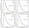 |
Fig. 11. Fits to the late-time SED of NGC 300 OT obtained 761 days after maximum. In the different panels are reported the fits for the different dust compositions and grain sizes. The best fit to the data is shown as a solid blue line, while the dashed lines show the effect of changes in the optical depth while keeping temperature and radius of the source fixed. |
Parameters obtained from fitting the SED of NGC 300 OT at 761 d.
Here we are assuming a constant density profile in the dust cloud, which is an additional approximation. Depending on the composition and grain size considered, the inferred dust mass spans from 4.4 × 10⁻⁵ M⊙ up to 2.0 × 10⁻³ M⊙ (see Table 2). It is interesting to note that these values, obtained at ∼800 days after explosion, are perfectly in line with the amount of dust found in the ejecta of core-collapse SNe6 (e.g. Fabbri et al. 2011; Bevan et al. 2020). We note that this fitting procedure was performed on the dust which was identified by Prieto et al. (2009) 93 days after discovery at a temperature of 1510 K (and named warm dust), and whose cooling is tracked in the upper panel of Figure 9. The initial temperature of this dust component is close to the dust sublimation temperature: this behaviour is compatible with newly formed dust which condensed few months after the peak luminosity of NGC 300 OT, and by the time of our fit has cooled down to ∼590 K. Similarly, also the third blackbody component with a temperature of 485 K detected by Prieto et al. (2009) at 93 days (identified as circumstellar dust that survived the explosion) must have cooled down, and the peak of its emission has shifted outside the monitored domain. As mentioned above, this component may be the origin of the exceeding flux observed at 22 μm.
We replicated this SED analysis on AT 2019abn, thanks to publicly available images of M51 taken by the JWST on 2022 December 13 (proposal 1240, PI M.E. Ressler), 2023 June 08, 2023 June 14 (proposal 1783 PI A. Adamo) and 2024 May 31 (3435 PI K.M. Sandstrom). The object is still visible even five years after its peak luminosity: we report the magnitudes obtained with PSF fitting through ECSNOOPY in the online supplementary material. The wavelength coverage of the first three epochs is too scarce to provide a well sampled SED, therefore we focused on the measurements obtained on 2024 May 31, 1956 days after discovery. To fill the gap between the F430M and F1000W filters, we inferred the behaviour of the F560W and F770W filters observed the previous year (2023 June 08). To do so, we assumed a constant colour evolution using the filters F444W (observed on 2023 June 08) and F430M (observed on 2024 May 31) as anchors. The flux in these overlapping filters decreases by a factor of 1.5 between the two epochs, and we assume that the same holds true for the F560W and F770W filters. Since cooling objects tend to become redder, this is likely an underestimation of the fluxes in F560W and F770W on 2024 May 31, yet this simple approximation allowed us to constrain a crucial spectral region of the target. The resulting SED is displayed in Figure 12. Firstly, we point out that the Paα line is located within the F182M filter, and this could account for the relative brightness of the transient in this band, which is therefore excluded from the following discussion.
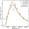 |
Fig. 12. SED of AT 2019abn 1956 days after discovery. The circles represent flux measurements obtained with JWST on 2024 May 31, while the squares represent data extrapolated from the measurements on 2023 June 08. The solid lines are the best fits for dust with different composition and grain size. |
In Figure 12 we show as solid lines the various fits to the observed SED of AT 2019abn with dust models characterised by different chemical composition and grain size. Parameters of each fit are shown in Table 3. The luminosity of the transient is found to be (2.8 ± 0.1)× 1038 erg s−1 (in Figure A.2 this result is added to the bolometric light curve of AT 2019abn, updating Figure 10). There is a discrepancy in the resulting temperature and radius depending on the dust composition: in the case of graphite, the best fits yield a temperature of ∼350 K and a radius of ∼350 AU, while for the silicate dust the temperature found is ∼370 K, with a blackbody radius of ∼300 AU. Grain size only plays a marginal role in shaping these results. Graphite dust models yield high optical depth (τ5 ≫ 1), leading to infer lower limits to the dust masses in the order of several 10−3 M⊙. On the other hand, the best-fitting silicate dust models are closer to the optically thin regime (τ5 ∼ 1), with inferred dust masses of the order of ∼2 × 10⁻⁴ M⊙. These results, however, need to be interpreted with caution, since even the best fits struggle to accurately reproduce the observed data. The observed departure from a simple blackbody is likely due to the presence of polycyclic aromatic hydrocarbons (PAHs). Rose et al. (2024) present a JWST spectrum of AT 2019abn taken on 2022 December 13, 18 months earlier than the SED shown in Figure 12, and they find two strong broad features at 6.3 μm and 8.25 μm which are identified as class C PAH. This is quite relevant in the characterisation of ILRTs: the observations of PAH in AT 2019abn by Rose et al. (2024) corroborate the identification of PAH in the MIR spectrum of NGC 300 OT by Prieto et al. (2009). The presence of class C PAH heavily favours a carbon-rich environment for AT 2019abn, NGC 300 OT, and by extension all ILRTs. Rose et al. (2024) also note that class C PAH are commonly found in post-AGB sources, compatibly with an ECSN origin for these objects. Accurate PAH modelling is beyond the scope of this study and is deferred to later works. Beyond these considerations on the shape of the SED, JWST observations provide valuable information on the MIR luminosity evolution of AT 2019abn five year after its discovery, as discussed in the following section.
Parameters obtained from fitting the SED of AT 2019abn at 1956 d.
6.2. Photometric decline below progenitor luminosity
Adams et al. (2016), monitored the two ILRTs NGC 300 OT and SN 2008S with the Spitzer telescope for several years, until they both faded below the luminosity of their respective progenitor. We update this follow-up campaign by analysing the Spitzer images collected between 2015 October 20 and 2019 November 24 with the Spitzer [4.5] μm channel. A visual inspection of the images shows that NGC 300 OT has faded below the detection threshold (Figure 13, left panel). We measure the flux on all public Spitzer [4.5] μm images through PSF fitting employing ECSNOOPY. Our results are in good agreement with the values measured with aperture photometry by Adams et al. (2016), with the exception of the very last detection, on 2015 February 09: we find a value of 600 ± 300 L⊙ against the 140 ± 110 L⊙ obtained with aperture photometry (the difference can be appreciated on the right panel of Figure 13). The complex background surrounding the target, as seen in the left panel of Figure 13, contributes to the uncertainty of this measure. All the images collected from that moment only provide upper limits to the luminosity of NGC 300 OT: in particular, in the right panel of Figure 13 we show the 1σ limits obtained from PSF fitting. We therefore confirm that since 2015 NGC 300 OT has faded below the detection threshold, well below the progenitorluminosity.
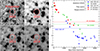 |
Fig. 13. Late-time MIR evolution of ILRTs. Left panel: Images of NGC 300 OT in the [4.5] μm channel of Spitzer from the progenitor until the disappearance of the transient. Right panel: Updated version of the figure shown in Adams et al. (2016), with their measurements in the [4.5] μm channel shown as circles. Additional data points for NGC 300 OT and AT 2019abn are shown as stars (upper limits are represented as empty symbols). We also show the JWST data point of AT 2019abn obtained by Rose et al. (2024). The progenitor luminosity of each transient is shown as a horizontal dashed line. |
We are also able to include AT 2019abn among the ILRTs with MIR coverage spanning several years. The light curve up to ∼500 days is provided by the Spitzer and WISE monitoring already shown in Figure 1, while the last two epochs are provided by the late JWST observations obtained 1598 and 1956 days after discovery and presented in the previous section. Despite the slight mismatch in the covered wavelength, the JWST filters F444W and F430M are sufficiently close to the [4.5] μm and W2 filters to provide a coherent light curve, which is shown with red stars symbols in Figure 13. The behaviour of AT 2019abn is similar to that of SN 2008S, where the initial decline rate significantly slows down after ∼200 days. It is interesting to consider the evolution of the transient compared to its progenitor luminosity in the [4.5] μm channel provided by Jencson et al. (2019), which is marked in Figure 13 as a red horizontal dashed line. It is possible to notice that on 2023 June 08 AT 2019abn has already faded below its progenitor luminosity, with the latest measure obtained on 2024 May 31 being over two times dimmer than the luminosity of the star before the event. All three ILRTs that were monitored for multiple years in the MIR domain eventually became dimmer than their progenitor star, and so far none of them has shown sign of stopping their steady luminosity decline: this fact supports the interpretation that ILRTs are terminal events.
7. Template light curve
In order to better characterise this class of objects, we produce an r band template light curve for ILRTs. We are also motivated by the potential usefulness of these templates in our future attempts to classify new transients discovered by the Vera Rubin Observatory (formerly Large Synoptic Survey Telescope, Ivezić et al. 2019) and released by dedicated science brokers such as Lasair (Smith et al. 2019) and Alerce (Förster et al. 2021). With the foreseen amount of data, it will be impossible to study in detail every single target, and template light curves for different classes of transient could prove to be useful tools for filtering the data stream, in addition to the classification algorithms and tools that are currently being developed (e.g. Fraga et al. 2024; de Soto et al. 2024). Apart from NGC 300 OT, AT 2019abn, AT 2019ahd and AT 2019udc, which were presented above, we broaden our sample including SN 2002bu (Smith et al. 2011), SN 2008S (Botticella et al. 2009), AT 2017be (Cai et al. 2018), SNHunt120 (Stritzinger et al. 2020), AT 2010dn, AT 2013jc, AT 2013la, AT 2013lb, AT 2018aes (Cai et al. 2021), and AT 2022fnm (Moran et al. 2024). We chose to focus on the r-band, since it is typically well-sampled and allows for a reliable comparison between objects. The peak absolute magnitude of different ILRTs can span at least three magnitudes (from −12 mag to −15 mag, see Figure 5): however, here we are interested in recovering just the expected light curve shape of ILRTs. For this reason we normalised the peak magnitude of all objects considered to the same arbitrary value. Both the light curve shape and the absolute magnitude at peak can then be used as filters to identify future ILRTs candidates.
As a first step to produce a light curve template we made use of Gaussian Processes to interpolate the light curves of each object (see e.g. Inserra et al. 2018 for a more detailed description of the procedure). In particular, we employed the MATERN 3/2 kernel found in the PYTHON package GEORGE (Ambikasaran et al. 2015), and as for the mean function we adopted equation 1 given by Bazin et al. (2011). It is worth noting that we performed the interpolation procedure in the “luminosity – time” space. Given the different sampling of each event, this first step was performed to ensure that each objects holds the same weight in the construction of the template, regardless of how many data points were collected at a given phase. After interpolating the light curve of each object, we recovered the mean value and the standard deviation of the ILRTs luminosity within temporal bins of 3 days, which we empirically chose as a good compromise that yields a rather smooth template which still has a reasonable time resolution. The resulting template light curve of an ILRT is shown as a black solid line in the upper panel of Figure 14, with the grey shaded area representing the 1 σ deviation from the mean.
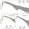 |
Fig. 14. Template light curves obtained for ILRTs. The solid black line represents the ILRTs template light curve, while the grey shaded area shows the 1σ deviation from the mean. The coloured dashed lines display the interpolation performed on each object. In the bottom panels the ILRTs are separated between slow and fast declining objects. |
Due to the low number of available ILRTs, the rising part of the template becomes reliable only at about −10 days with respect to maximum luminosity: before that phase the template is dominated by the widely different behaviours of AT 2019abn and AT 2018aes. The overall template light curve rises of about 0.5 mag from −10 days to 0 days, and fades by 1 mag from maximum to 50 days. As time progresses, the 1σ region gets wider, with objects evolving at different rates. Objects fading below the detection threshold can result in a jagged profile of the template, as happens at about 100 days due to the disappearing of AT 2018aes and AT 2022fnm. There is a variety of properties in the light curves of the considered ILRTs, but we can roughly divide them in two subclasses, based on their behaviour in the 50 days after maximum. The first group of objects present slowly declining, convex light curves, which on average only fade by 0.8 mag from day 0 to day 50. The second group of objects display fast declining, concave light curves, which on average fade by more than 1.3 mag in the same time span (see Figure 14, lower panels). While this distinction is clear in some cases (AT 2019abn and AT 2019ahd are slow decliners, while AT 2019udc and AT 2022fnm are fast decliners), there are some objects with intermediate properties, such as AT 2013la, whose light curve quickly fades in the first two months, only to flatten after 75 d, ultimately becoming even brighter than AT 2019abn after 130 d. Another outlier is AT 2018aes, which is characterised by the shallowest rise to maximum light, followed by a rather standard slow decline for 40 days before abruptly fading by 3.2 mag in 60 days. The dichotomy between slow and fast declining ILRTs is reminiscent of the division between SNe IIP and IIL (e.g. Anderson et al. 2014), with the progenitors of the slow declining ILRTs retaining larger hydrogen envelopes compared to the progenitors of fast declining ILRTs. A larger sample of ILRTs is needed to verify if this analogy holds true or if it is a mere coincidence.
8. A toy model for ILRTs light curves
In this section we present a simple model in the attempt to reproduce the shape of the bolometric light curves of ILRTs in the context of a weak SN explosion. The end goal is to obtain a rough estimate of parameters such as the amount of mass ejected and its velocity. The basic concepts are taken from Chatzopoulos et al. (2012), which in turn expand the approach introduced by Arnett (1980, 1982). First of all, 56Ni radioactive decay is expected to be a relevant power source for SNe, and its luminosity over time is given by the equation
![Mathematical equation: $$ \begin{aligned} L_{\rm Ni}(t)&= \frac{2M_{\rm Ni}}{t_{d}}e^{-\left[\frac{t^{2}}{t^{2}_{d}} + \frac{2R_{0}t}{vt^{2}_{d}}\right]}\left[(\epsilon _{\rm NI}-\epsilon _{Co}) \right.\nonumber \\&\times \int ^{t}_{0}\left[\frac{R_{0}}{vt_{d}} +\frac{t^{\prime }}{t_{d}}\right]e^{[\frac{t^{\prime 2}}{t^{2}_{d}} + \frac{2R_{0}t^{\prime }}{vt^{2}_{d}}]}e^{-t^{\prime }/t_{Ni}}dt^{\prime } \nonumber \\&\left. + \epsilon _{Co}\int ^{t}_{0}\left[\frac{R_{0}}{vt_{d}} +\frac{t^{\prime }}{t_{d}}\right]e^{\left[\frac{t^{\prime 2}}{t^{2}_{d}} + \frac{2R_{0}t^{\prime }}{vt^{2}_{d}}\right]}e^{-t^{\prime }/t_{Co}}dt^{\prime }\right](1-e^{-At^{-2}}) , \end{aligned} $$](/articles/aa/full_html/2025/03/aa51733-24/aa51733-24-eq8.gif) (2)
(2)
where MNi is the mass of synthesised 56Ni, tNi and tCo are the half lives of 56Ni and 56Co, while ϵNi and ϵCo are the energy generation rates of 56Ni and 56Co released during the radioactive decay. A is a constant that accounts for the opacity of the ejecta to γ-rays, with large values of A corresponding to complete trapping. The constant values are the same reported in Chatzopoulos et al. (2012). This equation takes into account the diffusion time through an homologously expanding gas of mass M, initial radius R0 and characteristic expansion velocity v. As discussed in Paper II, the velocity inferred from the width of the emission lines of our sample of ILRTs can reach only up to ∼103 km s−1. However, the observed emission lines of ILRTs originate in a dense CSM which is obscuring the underlying material: as happens for SNe IIn, fast ejecta may be hiding below this layer of dense gas. Theoretical expectations for ECSNe suggest that their ejecta should be less energetic than a standard SN (v ≲ 104 km s−1). The characteristic timescale td of the light curve can be written as a combination of the diffusion timescale t0 and the hydrodynamical timescale th:
 (3)
(3)
Here β is a constant linked to the density profile of the mass, and k is the opacity of the ejecta, for which we adopted a value of 0.33 cm2 g−1.
As an additional source of luminosity, we considered the radiation emitted by the expanding and cooling gas, which was heated by the blast wave that followed the explosion. This term was already introduced by Arnett (1980) to reproduce the slowly declining light curves of SNe IIP. Using the formalism of Chatzopoulos et al. (2012), this luminosity term can be written as
![Mathematical equation: $$ \begin{aligned} L_{\rm blast}(t) = \frac{E_{\rm th}}{t_{0}} e^{-\left[\frac{t^{2}}{t^{2}_{d}} + \frac{2R_{0}t}{vt^{2}_{d}}\right]}, \end{aligned} $$](/articles/aa/full_html/2025/03/aa51733-24/aa51733-24-eq10.gif) (4)
(4)
where Eth is the internal energy which was deposited in the ejecta during the explosion. To better reproduce the observed shape of the light curve, we considered two blast terms: one associated with the envelope, less massive and more extended, characterised by a short diffusion time, and another associated with the bulk of the ejecta, more massive and dense, with a much longer diffusion timescale. Dividing the ejecta in two regions is not a novelty: this approach has been successfully used, for example, by Nagy & Vinkó (2016). The total time dependent luminosity is therefore the sum of these three contributions:
 (5)
(5)
The final piece of the model is the thick CSM surrounding the transient, which is a key feature observed in ILRTs spectra. This element does not provide additional energy, but it simply reprocesses the total luminosity emitted by the ejecta and 56Ni, delaying its appearance. To reproduce this effect, we made use of the fixed photosphere approximation presented by Chatzopoulos et al. (2012)
 (6)
(6)
where tCSM is the diffusion time through the thick CSM shell surrounding the transient. Its effect is crucial in the first phases, during which the blast terms Lbulk and Lenvelope start abruptly from the maximum luminosity, without a rising phase. A CSM shell with a diffusion time of few days allow the model to reproduce the rise observed in ILRTs. In Figure 15 are shown the models and the bolometric light curves they are trying to emulate. The contribution of each component is shown with different colours: the parameters relative to each of them are reported in Table 4. One weakness of this approach is the assumption of spherical symmetry, which may be a crude approximation in the case of these transients (e.g. Soker & Kashi 2012). An additional fragility is the large number of free parameters, as well as the degeneracy between some of them: similar solutions can be obtained while inputting different parameters. A relevant degeneracy is found between the characteristic velocity of the ejecta and their mass, since the same diffusion time can be obtained by either increasing or decreasing both the mass and velocity of the ejecta. In such cases, spectroscopic observations may provide useful constraints on the velocities to input in the models. In the case of ILRTs, the velocities inferred from the full width at half maximum of the lines is typically below ∼1000 km s−1; however, as discussed in Paper II, this observation does not exclude the presence of faster ejecta located underneath the CSM, as happens for type IIn SNe. Our main goal in this section is to evaluate if the bolometric light curves of ILRTs are compatible with weak SN events. We therefore try to find models with kinetic energy of a few 1050 erg, as expected for ECSNe explosions (Janka et al. 2008). This choice will inevitably lead to infer ejecta velocities larger than the ones measured on the spectra of ILRTs, with the idea that this faster ejecta should lie below a layer of CSM, responsible for the emission of the narrow lines. For completeness, at the end of this section we also report the ejected masses obtained by adopting the velocities measured from the narrow lines in the spectra of our ILRTs: these values can provide reasonable lower limits to the masses ejected during these events.
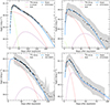 |
Fig. 15. Bolometric light curves of our sample of ILRTs (represented as black circles) with a toy model reproducing their shape. The errors on the data points, dominated by the uncertainty on distance and reddening estimations, are reported as a grey shaded area. The toy models attempting to reproduce the behaviour of each transient is shown as a solid light blue line. The energy sources powering the different phases of the light curves are shown as dashed lines. |
AT 2019abn is definitely the most successful example within our sample. The emission from a rather massive envelope of 1 M⊙, combined with a CSM diffusion time of 10 days, seems
to properly reproduce the rise and the maximum phases. The subsequent slow decline can be explained by 7 M⊙ of ejecta moving with a characteristic velocity of
1900 km s−1, leading to a rather large diffusion time and a photospheric phase lasting around 200 days. The 56Ni contribution is not significant until the
late phases, and it is definitely too faint to explain the evolution after 200 days: as mentioned in the previous section, an additional source of energy is likely needed to explain the late-time luminosity of ILRTs. The parameters used to model AT 2019ahd do not differ significantly from the ones used for AT 2019abn: they are mainly scaled down in mass (4 M⊙ of ejecta in total) and internal energy of the ejecta. The blast term associated with the envelope is not as crucial, but the overall evolution appears to be reproduced sufficiently well, excluding the late shallow decline. The larger characteristic velocity 4500 km s−1 and lower ejected mass compared to AT 2019abn leads to a shorter diffusion time, with the energy released by 56Ni decay becoming relevant around 60 days after explosion. Since we miss the first evolutionary phases of NGC 300 OT, we only use a single blast term (associated with the bulk of the ejecta) plus 56Ni decay to reproduce the data: the blast term associated with the envelope is relevant during the early phases, so it is difficult to constrain in this case. Apart from this, the parameters used for NGC 300 OT are very similar to the ones used for AT 2019ahd, except for a slightly lower characteristic velocity of 3500 km s−1, and a marginally larger ejected mass of 4.2 M⊙, leading to a longer photon diffusion time through the ejecta. The same conclusions cannot be reached for AT 2019udc, which is definitely an outlier in this sample. First of all, the fast decline hints at the presence of a single blast term. Most strikingly, the evolution of AT 2019udc is much faster compared to the other transients considered so far. For this reason the diffusion time within the ejecta must be much lower: this leads to a low ejected mass and a high scale velocity, several times higher compared to the other ILRTs mentioned so far. Finally, it is worth noticing that in the case of AT 2019udc, 56Ni decay is a key element to reproduce the observed late-time data points, but it also becomes the dominant contribution within three weeks after explosion, much earlier compared to other ILRTs studied.
All the masses mentioned so far are just relative to the ejected material: in the scenario in which ILRTs arise from a core collapse event, a compact remnant is expected to be left behind. Since the mass of the remnant can be estimated to be 1.3–2.0 M⊙ (Pumo et al. 2017), the inferred mass of our sample of ILRTs right before the explosion adds up to 5.3–6.0 M⊙ for AT 2019ahd, 5.5–6.2 M⊙ for NGC 300 OT and 9.3–10 M⊙ for AT 2019abn. These values are compatible with the expectations for SAGB stars and consequently ECSN events, especially accounting for the fact that some mass was likely lost during the evolution of the star, therefore leading to a slightly higher ZAMS. AT 2019udc, with its estimated progenitor mass of just 2.2–2.9 M⊙ at the time of explosion, sets itself apart from the rest of the sample, although its origin could be tentatively explained as an ECSN arising from a SAGB star that underwent extreme mass loss. This scenario, however, needs to be more thoroughly explored, since within the present model AT 2019udc struggles to be reconciled with an ECSN event. We note that the toy model presented in this section is a simplified approach to the light curve modelling of ILRTs: more detailed models envisioning hydrodynamical modelling should be used to retrieve more robust estimates of the explosion parameters of these objects. Accounting for the possible luminosity contribution from ejecta-CSM interaction will also be an important step forward: while ILRTs never display spectral signatures typically associated with strong shocks, there may be hidden CSM interaction powering their light curve (Paper II). The puzzling results obtained for AT 2019udc may be significantly revised by using a more refined approach.
As a final application, we can use the model described above to provide lower limits to the masses ejected during the observed events. To do so, instead of placing constraints on the kinetic energy of each object to reproduce the expected values of a weak SNe event, we adopt the observed velocities of each object (Figure 7 in Paper II) as characteristic ejecta velocity in the models. Due to the degeneracy between mass and velocity mentioned above, we can find models that reproduce the data as shown in Figure 15 by adjusting the ejected mass accordingly. The masses needed to reproduce the bolometric light curves in these conditions provide a lower limit to the ejected mass, based on the fact that the characteristic velocity of the ejecta could be higher than the observed ones (if fast ejecta lie beneath the CSM), but cannot be lower. Here we present the resulting masses for each transient, with the adopted characteristic velocity in brackets: 2.6 M⊙ for AT 2019abn (v ∼ 700 km s−1), 0.7 M⊙ for AT 2019ahd (v ∼ 700 km s−1), 0.8 M⊙ for NGC 300 OT (v ∼ 600 km s−1) and 0.05 M⊙ for AT 2019udc (v ∼ 600 km s−1). We note that our lower mass limit obtained for NGC 300 OT fulfils the lower limit on the ejected mass of ≳0.25 M⊙ provided by Kochanek (2011) based on considerations on the late-time shock luminosity.
9. Summary and conclusions
In this work we present datasets for NGC 300 OT, AT 2019abn, AT 2019ahd, and AT 2019udc. AT 2019abn and AT 2019udc stand out for their bright peak magnitude (Mr = −14.7 mag and −14.2 mag respectively). On the other hand, NGC 300 OT and AT 2019ahd are characterised by a more modest peak magnitude (Mr = −12.9 mag and −13.0 mag). We detect a NIR excess in the SEDs of three of our ILRTs, AT 2019abn, AT 2019ahd, and NGC 300 OT, tentatively associated with dust formation. At late phases, the contributions in the NIR and MIR domains to the bolometric light curve cause a decline shallower than the luminosity decline supported by the 56Ni decay, hinting at the presence of an additional powering mechanism. As suggested by Kochanek (2011), this could be a sign of shocks sweeping the dust surrounding the transients. The only exception we have found so far is AT 2019udc, which shows a late-time decline perfectly described by the radioactive decay of 3.3 × 10⁻³ M⊙ of 56Ni. We also note that AT 2019udc displays the fastest evolution timescale among the ILRTs observed, making it a peculiar object within a peculiar class.
The late-time monitoring of NGC 300 OT with WISE allows us to build the SED of the transient 761 days after maximum. From its study, we infer a dust mass of the order of 10−5–10−3 M⊙, depending on the composition and size of the grains adopted. Furthermore, the evolution of NGC 300 OT has been monitored with Spitzer for several years, showing a steady dimming of the flux at the transient position over 4 years. This strengthens the argument suggested by Adams et al. (2016) that NGC 300 OT was a terminal event. Thanks to JWST observations, we were able to show that AT 2019abn also faded below its progenitor luminosity in the MIR domain. Its SED appears to depart from a simple blackbody, possibly due to the presence of PAH emission features. Finally, a simple model is presented in the context of a SN explosion, with the goal of estimating the parameters that characterise the transients. For AT 2019abn, 2019ahd, and NGC 300 OT, the low masses ejected (between 4 and 8 M⊙) and low velocity of the material (up to 5000 km s−1) are compatible with a weak explosion from a low-mass star. AT 2019udc is an outlier in this sense since its very fast decline rate leads to inferring high velocity (12 000 km s−1) and a remarkably low ejected mass (0.9 M⊙), which would suggest a different type of event. However, accurate hydrodynamical modelling and taking into account the role of ejecta-CSM interaction will indubitably help with the analysis and interpretation of this transient and the whole class of objects. Overall, due to their low energy and their likely terminal nature inferred from their MIR decline, ILRTs remain solid candidates for being ECSNe.
Data availability
The tables from Appendix A and B containing the data presented in this article are available at the CDS via anonymous ftp to cdsarc.cds.unistra.fr (130.79.128.5) or via https://cdsarc.cds.unistra.fr/viz-bin/cat/J/A+A/695/A42
Acknowledgments
We thank the staff of the various observatories where data were obtained for their assistance. Based on observations made with the Nordic Optical Telescope, owned in collaboration by the University of Turku and Aarhus University, and operated jointly by Aarhus University, the University of Turku and the University of Oslo, representing Denmark, Finland and Norway, the University of Iceland and Stockholm University at the Observatorio del Roque de los Muchachos, La Palma, Spain, of the Instituto de Astrofisica de Canarias. Observations from the Nordic Optical Telescope were obtained through the NUTS2 collaboration which are supported in part by the Instrument Centre for Danish Astrophysics (IDA). The data presented here were obtained in part with ALFOSC, which is provided by the Instituto de Astrofisica de Andalucia (IAA). This work makes use of data from the Las Cumbres Observatory network. The LCO team is supported by NSF grants AST–1911225 and AST–1911151, and NASA SWIFT grant 80NSSC19K1639. Data were also obtained at the Liverpool Telescope, which is operated on the island of La Palma by Liverpool John Moores University in the Spanish Observatorio del Roque de los Muchachos with financial support from the UK Science and Technology Facilities Council. Part of the observations were collected at Copernico and Schmidt telescopes (Asiago, Italy) of the INAF – Osservatorio Astronomico di Padova. Based on observations made with the Gran Telescopio Canarias (GTC), installed in the Spanish Observatorio del Roque de los Muchachos of the Instituto de Astrofisica de Canarias, in the island of La Palma This work has made use of data from the Asteroid Terrestrial-impact Last Alert System (ATLAS) project. Time domain research by the University of Arizona team and D.J.S. is supported by NSF grants AST-1821987, 1813466, 1908972, & 2108032, and by the Heising-Simons Foundation under grant #20201864. G.V., N.E.R. and I.S. acknowledge financial support from PRIN-INAF 2022 “Shedding light on the nature of gap transients: from the observations to the models”. N.E.R. also acknowledge support from the Spanish MICINN grant PID2019-108709GB-I00 and FEDER funds, and from the program Unidad de Excelencia Maria de Maeztu CEX2020-001058-M. A.R. acknowledges financial support from the GRAWITA Large Program Grant (PI P. D’Avanzo) and the PRIN-INAF 2022 “Shedding light on the nature of gap transients: from the observations to the models”. Y.-Z. Cai is supported by the National Natural Science Foundation of China (NSFC, Grant No. 12303054), the Yunnan Fundamental Research Projects (Grant No. 202401AU070063) and the International Centre of Supernovae, Yunnan Key Laboratory (No. 202302AN360001). T.E.M.B. acknowledges financial support from the Spanish Ministerio de Ciencia e Innovacion (MCIN), the Agencia Estatal de Investigacion (AEI) 10.13039/501100011033, and the European Union Next Generation EU/PRTR funds under the 2021 Juan de la Cierva program FJC2021-047124-I and the PID2020-115253GA-I00 HOSTFLOWS project, from Centro Superior de Investigaciones Cientificas (CSIC) under the PIE project 20215AT016, and the program Unidad de Excelencia Maria de Maeztu CEX2020-001058-M. MF is supported by a Royal Society – Science Foundation Ireland University Research Fellowship. The Aarhus supernova group is funded by the Independent Research Fund Denmark (IRFD, grant numbers 8021-00170B, 10.46540/2032-00022B). L.G. acknowledges financial support from the Spanish Ministerio de Ciencia e Innovación (MCIN), the Agencia Estatal de Investigación (AEI) 10.13039/501100011033, and the European Social Fund (ESF). This work was funded by ANID, Millennium Science Initiative, ICN12_009 M.N. is supported by the European Research Council (ERC) under the European Union’s Horizon 2020 research and innovation programme (grant agreement No. 948381). Part of the funding for GROND (both hardware as well as personnel) was generously granted from the Leibniz-Prize to Prof. G. Hasinger (DFG grant HA 1850/28-1). H.K. was funded by the Academy of Finland projects 324504 and 328898. R.K. acknowledges support from the Research Council of Finland (340613).
References
- Adams, S. M., Kochanek, C. S., Prieto, J. L., et al. 2016, MNRAS, 460, 1645 [NASA ADS] [CrossRef] [Google Scholar]
- Ambikasaran, S., Foreman-Mackey, D., Greengard, L., Hogg, D. W., & O’Neil, M. 2015, IEEE Trans. Pattern Anal. Mach. Intell., 38, 252 [Google Scholar]
- Anderson, J. P., González-Gaitán, S., Hamuy, M., et al. 2014, ApJ, 786, 67 [Google Scholar]
- Arnett, W. D. 1980, ApJ, 237, 541 [Google Scholar]
- Arnett, W. D. 1982, ApJ, 253, 785 [Google Scholar]
- Bazin, G., Ruhlmann-Kleider, V., Palanque-Delabrouille, N., et al. 2011, A&A, 534, A43 [NASA ADS] [CrossRef] [EDP Sciences] [Google Scholar]
- Berger, E., Soderberg, A. M., Chevalier, R. A., et al. 2009, ApJ, 699, 1850 [NASA ADS] [CrossRef] [Google Scholar]
- Bevan, A. M., Krafton, K., Wesson, R., et al. 2020, ApJ, 894, 111 [NASA ADS] [CrossRef] [Google Scholar]
- Bond, H. E., Bedin, L. R., Bonanos, A. Z., et al. 2009, ApJ, 695, L154 [Google Scholar]
- Botticella, M. T., Pastorello, A., Smartt, S. J., et al. 2009, MNRAS, 398, 1041 [NASA ADS] [CrossRef] [Google Scholar]
- Branch, D., & Wheeler, J. C. 2017, Supernova Explosions (Springer-Verlag GmbH Germany) [CrossRef] [Google Scholar]
- Byrne, R. A., Fraser, M., Cai, Y. Z., Reguitti, A., & Valerin, G. 2023, MNRAS, 524, 2978 [NASA ADS] [CrossRef] [Google Scholar]
- Cai, Y. Z., Pastorello, A., Fraser, M., et al. 2018, MNRAS, 480, 3424 [NASA ADS] [Google Scholar]
- Cai, Y. Z., Pastorello, A., Fraser, M., et al. 2021, A&A, 654, A157 [NASA ADS] [CrossRef] [EDP Sciences] [Google Scholar]
- Cappellaro, E. 2014, http://sngroup.oapd.inaf.it/snoopy.html [Google Scholar]
- Cardelli, J. A., Clayton, G. C., & Mathis, J. S. 1989, ApJ, 345, 245 [Google Scholar]
- Chambers, K. C., Magnier, E. A., Metcalfe, N., et al. 2016, arXiv e-prints [arXiv:1612.05560] [Google Scholar]
- Chatzopoulos, E., Wheeler, J. C., & Vinko, J. 2012, ApJ, 746, 121 [Google Scholar]
- de Soto, K., Villar, V. A., Lincc-Frameworks, et al. 2024, Am. Astron. Soc. Meeting Abstr., 243, 261.29 [NASA ADS] [Google Scholar]
- de Vaucouleurs, G., de Vaucouleurs, A., Corwin, H. G. J., et al. 1991, Third Reference Catalogue of Bright Galaxies (New York, NY: Springer) [Google Scholar]
- Dessart, L., Hillier, D. J., Audit, E., Livne, E., & Waldman, R. 2016, MNRAS, 458, 2094 [Google Scholar]
- Doherty, C. L., Gil-Pons, P., Siess, L., Lattanzio, J. C., & Lau, H. H. B. 2015, MNRAS, 446, 2599 [Google Scholar]
- Draine, B. T. 1989, in Infrared Spectroscopy in Astronomy, ed. E. Böhm-Vitense, 93 [Google Scholar]
- Draine, B. T. 2016, ApJ, 831, 109 [NASA ADS] [CrossRef] [Google Scholar]
- Draine, B. T., & Lee, H. M. 1984, ApJ, 285, 89 [NASA ADS] [CrossRef] [Google Scholar]
- Fabbri, J., Otsuka, M., Barlow, M. J., et al. 2011, MNRAS, 418, 1285 [CrossRef] [Google Scholar]
- Fixsen, D. J., Cheng, E. S., Gales, J. M., et al. 1996, ApJ, 473, 576 [Google Scholar]
- Förster, F., Cabrera-Vives, G., Castillo-Navarrete, E., et al. 2021, AJ, 161, 242 [CrossRef] [Google Scholar]
- Fox, O. D., Chevalier, R. A., Dwek, E., et al. 2010, ApJ, 725, 1768 [NASA ADS] [CrossRef] [Google Scholar]
- Fraga, B. M. O., Bom, C. R., Santos, A., et al. 2024, A&A, 692, A208 [NASA ADS] [CrossRef] [EDP Sciences] [Google Scholar]
- Gardner, J. P., Mather, J. C., Clampin, M., et al. 2006, Space Sci. Rev., 123, 485 [Google Scholar]
- Gogarten, S. M., Dalcanton, J. J., Williams, B. F., et al. 2010, ApJ, 712, 858 [NASA ADS] [CrossRef] [Google Scholar]
- Graham, M. J., Kulkarni, S. R., Bellm, E. C., et al. 2019, PASP, 131, 078001 [Google Scholar]
- Greiner, J., Bornemann, W., Clemens, C., et al. 2008, PASP, 120, 405 [Google Scholar]
- Hamuy, M. 2003, ApJ, 582, 905 [NASA ADS] [CrossRef] [Google Scholar]
- Helou, G., Madore, B. F., Schmitz, M., et al. 1991, in Databases and On-line Data in Astronomy, eds. M. A. Albrecht, & D. Egret, Astrophys. Space Sci. Lib., 171, 89 [NASA ADS] [CrossRef] [Google Scholar]
- Hiramatsu, D., Howell, D. A., Van Dyk, S. D., et al. 2021, Nat. Astron., 5, 903 [NASA ADS] [CrossRef] [Google Scholar]
- Holmbo, S., Stritzinger, M., Nowack, G., et al. 2019, ATel, 12661, 1 [NASA ADS] [Google Scholar]
- Hosseinzadeh, G., Sand, D. J., Jencson, J. E., et al. 2023, ApJ, 942, L18 [NASA ADS] [CrossRef] [Google Scholar]
- Howell, D. 2019, Am. Astron. Soc. Meeting Abstr., 233, 258.16 [NASA ADS] [Google Scholar]
- Humphreys, R. M., Bond, H. E., Bedin, L. R., et al. 2011, ApJ, 743, 118 [NASA ADS] [CrossRef] [Google Scholar]
- Inserra, C., Prajs, S., Gutierrez, C. P., et al. 2018, ApJ, 854, 175 [NASA ADS] [CrossRef] [Google Scholar]
- Ivezić, Ž., Kahn, S. M., Tyson, J. A., et al. 2019, ApJ, 873, 111 [Google Scholar]
- Janka, H. T., Müller, B., Kitaura, F. S., & Buras, R. 2008, A&A, 485, 199 [NASA ADS] [CrossRef] [EDP Sciences] [Google Scholar]
- Jencson, J. E., Adams, S. M., Bond, H. E., et al. 2019, ApJ, 880, L20 [NASA ADS] [CrossRef] [Google Scholar]
- Jha, S. 2019, Trans. Name Server Class. Rep., 2019-1237, 1 [NASA ADS] [Google Scholar]
- Jiang, N., Dou, L., Wang, T., et al. 2016, ApJ, 828, L14 [Google Scholar]
- Jones, S., Hirschi, R., Nomoto, K., et al. 2013, ApJ, 772, 150 [NASA ADS] [CrossRef] [Google Scholar]
- Karachentsev, I., Lebedev, V., & Shcherbanovski, A. 1985, Bulletin d’Information du Centre de Donnees Stellaires, 29, 87 [Google Scholar]
- Karambelkar, V. R., Kasliwal, M. M., Blagorodnova, N., et al. 2023, ApJ, 948, 137 [NASA ADS] [CrossRef] [Google Scholar]
- Kashi, A., Frankowski, A., & Soker, N. 2010, ApJ, 709, L11 [NASA ADS] [CrossRef] [Google Scholar]
- Kochanek, C. S. 2011, ApJ, 741, 37 [NASA ADS] [CrossRef] [Google Scholar]
- Kozyreva, A., Baklanov, P., Jones, S., Stockinger, G., & Janka, H.-T. 2021, MNRAS, 503, 797 [NASA ADS] [CrossRef] [Google Scholar]
- Lacy, M., Wilson, G., Masci, F., et al. 2005, ApJS, 161, 41 [NASA ADS] [CrossRef] [Google Scholar]
- Landolt, A. U. 1992, AJ, 104, 340 [Google Scholar]
- Limongi, M., Roberti, L., Chieffi, A., & Nomoto, K. 2024, ApJS, 270, 29 [NASA ADS] [CrossRef] [Google Scholar]
- Mainzer, A., Bauer, J., Grav, T., et al. 2011, ApJ, 731, 53 [Google Scholar]
- McQuinn, K. B. W., Skillman, E. D., Dolphin, A. E., Berg, D., & Kennicutt, R. 2016, ApJ, 826, 21 [NASA ADS] [CrossRef] [Google Scholar]
- McQuinn, K. B. W., Skillman, E. D., Dolphin, A. E., Berg, D., & Kennicutt, R. 2017, AJ, 154, 51 [NASA ADS] [CrossRef] [Google Scholar]
- Miller, A. A., Smith, N., Li, W., et al. 2010, AJ, 139, 2218 [NASA ADS] [CrossRef] [Google Scholar]
- Miyaji, S., Nomoto, K., Yokoi, K., & Sugimoto, D. 1980, PASJ, 32, 303 [Google Scholar]
- Monard, L. A. G. 2008, Int. Astron. Union Circ., 8946, 1 [NASA ADS] [Google Scholar]
- Moran, S., Kotak, R., Fraser, M., et al. 2024, A&A, 688, A161 [NASA ADS] [CrossRef] [EDP Sciences] [Google Scholar]
- Moriya, T. J., Tominaga, N., Langer, N., et al. 2014, A&A, 569, A57 [NASA ADS] [CrossRef] [EDP Sciences] [Google Scholar]
- Nagy, A. P., & Vinkó, J. 2016, A&A, 589, A53 [NASA ADS] [CrossRef] [EDP Sciences] [Google Scholar]
- Nasonova, O. G., de Freitas Pacheco, J. A., & Karachentsev, I. D. 2011, A&A, 532, A104 [NASA ADS] [CrossRef] [EDP Sciences] [Google Scholar]
- Nomoto, K. 1984, ApJ, 277, 791 [NASA ADS] [CrossRef] [Google Scholar]
- Nugent, P. E., Sullivan, M., Cenko, S. B., et al. 2011, Nature, 480, 344 [NASA ADS] [CrossRef] [Google Scholar]
- Ohsawa, R., Sakon, I., Onaka, T., et al. 2010, ApJ, 718, 1456 [NASA ADS] [CrossRef] [Google Scholar]
- Osterbrock, D. E., & Ferland, G. J. 2006, Astrophysics of Gaseous Nebulae and Active Galactic Nuclei (Sausalito, CA: University Science Books) [Google Scholar]
- Pastorello, A., & Fraser, M. 2019, Nat. Astron., 3, 676 [Google Scholar]
- Pastorello, A., Sauer, D., Taubenberger, S., et al. 2006, MNRAS, 370, 1752 [NASA ADS] [CrossRef] [Google Scholar]
- Pastorello, A., Valenti, S., Zampieri, L., et al. 2009, MNRAS, 394, 2266 [Google Scholar]
- Pastorello, A., Chen, T. W., Cai, Y. Z., et al. 2019a, A&A, 625, L8 [NASA ADS] [CrossRef] [EDP Sciences] [Google Scholar]
- Pastorello, A., Mason, E., Taubenberger, S., et al. 2019b, A&A, 630, A75 [NASA ADS] [CrossRef] [EDP Sciences] [Google Scholar]
- Pastorello, A., Fraser, M., Valerin, G., et al. 2021, A&A, 646, A119 [EDP Sciences] [Google Scholar]
- Poelarends, A. J. T., Herwig, F., Langer, N., & Heger, A. 2008, ApJ, 675, 614 [Google Scholar]
- Poznanski, D., Prochaska, J. X., & Bloom, J. S. 2012, MNRAS, 426, 1465 [Google Scholar]
- Prieto, J. L. 2008, ATel, 1550, 1 [NASA ADS] [Google Scholar]
- Prieto, J. L., Sellgren, K., Thompson, T. A., & Kochanek, C. S. 2009, ApJ, 705, 1425 [NASA ADS] [CrossRef] [Google Scholar]
- Pumo, M. L., Turatto, M., Botticella, M. T., et al. 2009, ApJ, 705, L138 [NASA ADS] [CrossRef] [Google Scholar]
- Pumo, M. L., Zampieri, L., Spiro, S., et al. 2017, MNRAS, 464, 3013 [NASA ADS] [CrossRef] [Google Scholar]
- Reguitti, A., Pumo, M. L., Mazzali, P. A., et al. 2021, MNRAS, 501, 1059 [Google Scholar]
- Rieke, G. H., & Lebofsky, M. J. 1985, ApJ, 288, 618 [Google Scholar]
- Roming, P. W. A., Kennedy, T. E., Mason, K. O., et al. 2005, Space Sci. Rev., 120, 95 [Google Scholar]
- Rose, S., Lau, R. M., Jencson, J. E., et al. 2024, ApJ, submitted [arXiv:2407.20430] [Google Scholar]
- Schlafly, F., & Finkbeiner, D. P. 2011, ApJ, 737, 103 [NASA ADS] [CrossRef] [Google Scholar]
- Siebert, M. R., Dimitriadis, G., Kilpatrick, C. D., et al. 2019, Trans. Name Server Class. Rep., 2019-2287, 1 [NASA ADS] [Google Scholar]
- Skrutskie, M. F., Cutri, R. M., Stiening, R., et al. 2006, AJ, 131, 1163 [NASA ADS] [CrossRef] [Google Scholar]
- Smartt, S. J., Valenti, S., Fraser, M., et al. 2015, A&A, 579, A40 [NASA ADS] [CrossRef] [EDP Sciences] [Google Scholar]
- Smith, N. 2013, MNRAS, 434, 102 [Google Scholar]
- Smith, N., Ganeshalingam, M., Chornock, R., et al. 2009, ApJ, 697, L49 [Google Scholar]
- Smith, N., Li, W., Silverman, J. M., Ganeshalingam, M., & Filippenko, A. V. 2011, MNRAS, 415, 773 [NASA ADS] [CrossRef] [Google Scholar]
- Smith, K. W., Williams, R. D., Young, D. R., et al. 2019, Res. Notes Am. Astron. Soc., 3, 26 [Google Scholar]
- Smith, K. W., Smartt, S. J., Young, D. R., et al. 2020, PASP, 132, 085002 [Google Scholar]
- Soker, N., & Kashi, A. 2012, ApJ, 746, 100 [NASA ADS] [CrossRef] [Google Scholar]
- Spergel, D. N., Bean, R., Doré, O., et al. 2007, ApJS, 170, 377 [NASA ADS] [CrossRef] [Google Scholar]
- Spiro, S., Pastorello, A., Pumo, M. L., et al. 2014, MNRAS, 439, 2873 [Google Scholar]
- Steele, I. A., Smith, R. J., Rees, P. C., et al. 2004, in Ground-based Telescopes, eds. J. Oschmann, & M. Jacobus, SPIE Conf. Ser., 5489, 679 [NASA ADS] [CrossRef] [Google Scholar]
- Stritzinger, M. D., Taddia, F., Fraser, M., et al. 2020, A&A, 639, A103 [NASA ADS] [CrossRef] [EDP Sciences] [Google Scholar]
- Szczygieł, D. M., Prieto, J. L., Kochanek, C. S., et al. 2012, ApJ, 750, 77 [CrossRef] [Google Scholar]
- Tartaglia, L., Sand, D. J., Valenti, S., et al. 2018, ApJ, 853, 62 [Google Scholar]
- Thompson, T. A., Prieto, J. L., Stanek, K. Z., et al. 2009, ApJ, 705, 1364 [NASA ADS] [CrossRef] [Google Scholar]
- Tody, D. 1986, in Instrumentation in astronomy VI, ed. D. L. Crawford, SPIE Conf. Ser., 627, 733 [Google Scholar]
- Tonry, J. L., Denneau, L., Heinze, A. N., et al. 2018, PASP, 130, 064505 [Google Scholar]
- Tonry, J., Denneau, L., Heinze, A., et al. 2019, Trans. Name Server Discov. Rep., 2019-161, 1 [NASA ADS] [Google Scholar]
- Tully, R. B., & Fisher, J. R. 1988, Catalog of Nearby Galaxies (Cambridge, UK: Cambridge University Press) [Google Scholar]
- Tully, R. B., Shaya, E. J., & Pierce, M. J. 1992, ApJS, 80, 479 [NASA ADS] [CrossRef] [Google Scholar]
- Tully, R. B., Rizzi, L., Shaya, E. J., et al. 2009, AJ, 138, 323 [NASA ADS] [CrossRef] [Google Scholar]
- Turatto, M., Benetti, S., & Cappellaro, E. 2003, in From Twilight to Highlight: The Physics of Supernovae, eds. W. Hillebrandt, & B. Leibundgut, 200 [Google Scholar]
- Tylenda, R., Hajduk, M., Kamiński, T., et al. 2011, A&A, 528, A114 [NASA ADS] [CrossRef] [EDP Sciences] [Google Scholar]
- Valerin, G., Pumo, M. L., Pastorello, A., et al. 2022, MNRAS, 513, 4983 [NASA ADS] [CrossRef] [Google Scholar]
- Valerin, G., Pastorello, A., Mason, E., et al. 2024, A&A, in press https://doi.org/10.1051/0004-6361/202451735 (Paper II) [Google Scholar]
- Wanajo, S., Nomoto, K., Janka, H. T., Kitaura, F. S., & Müller, B. 2009, ApJ, 695, 208 [NASA ADS] [CrossRef] [Google Scholar]
- Wesson, R., Barlow, M. J., Matsuura, M., & Ercolano, B. 2015, MNRAS, 446, 2089 [NASA ADS] [CrossRef] [Google Scholar]
- Williams, S. C., Darnley, M. J., Bode, M. F., & Steele, I. A. 2015, ApJ, 805, L18 [Google Scholar]
- Williams, S. C., Jones, D., Pessev, P., et al. 2020, A&A, 637, A20 [NASA ADS] [CrossRef] [EDP Sciences] [Google Scholar]
- Woosley, S. E., Heger, A., & Weaver, T. A. 2002, Rev. Mod. Phys., 74, 1015 [NASA ADS] [CrossRef] [Google Scholar]
- Wright, E. L., Eisenhardt, P. R. M., Mainzer, A. K., et al. 2010, AJ, 140, 1868 [Google Scholar]
- York, D. G., Adelman, J., & Anderson, J. E. Jr 2000, AJ, 120, 1579 [NASA ADS] [CrossRef] [Google Scholar]
Appendix A: Additional figures
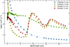 |
Fig. A.1. Opacity of dust with different compositions (graphite and silicates) and grain sizes (0.1 and 1 μm). The reported values were tabulated by Fox et al. (2010) and extended to 22 μm as detailed in Section 6.1. |
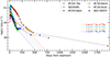 |
Fig. A.2. Updated version of Figure 10 including the late-time luminosity of AT 2019abn measured on JWST data collected on 2024 May 31. |
All Tables
All Figures
|
Fig. 1. Optical, NIR, and MIR light curves of AT 2019abn. The filled circles represent the unpublished data, while the empty circles represent the data points from the literature. The empty triangles represent the upper limits. |
| In the text | |
|
Fig. 2. Optical and NIR light curves of AT 2019ahd. Filled circles represent unpublished data, while empty circles represent ZTF data points. Empty triangles represent upper magnitude limits. Magnitude shifts on i and z bands have been applied for clarity. |
| In the text | |
|
Fig. 3. Photometric data collected for AT 2019udc. In the right panel we present optical and NIR light curves of AT 2019udc. Magnitude shifts have been applied for clarity. Filled circles represent unpublished data, while empty circles represent ZTF data points. In the left panels is shown DLT40 monitoring of AT 2019udc. In particular, in the upper left panel is shown the high-cadence follow-up of the rise of AT 2019udc. The DLT40 data points are shown as stars and are integrated with observations obtained through other facilities, represented as circles. In the lower left, years of upper limits collected by DLT40 are displayed as black triangles, with the detections of the transient appearing as green symbols at the right edge of the figure. |
| In the text | |
|
Fig. 4. UV, optical, and NIR light curves of NGC 300 OT. Empty triangles represent upper limits. Filled circles represent unpublished data, while empty circles represent publicly available SWIFT data. |
| In the text | |
|
Fig. 5. Absolute r band (upper panel) and H band (lower panel) light curve comparison between the ILRTs in our sample and other low-luminosity transients. In particular, ILRTs are marked with circles, LRNe with plus signs, and SN IIP with diamonds. |
| In the text | |
|
Fig. 6. Colour curves after reddening correction for the ILRTs belonging to our sample, with the addition of SN 2008S and AT 2017be. In the top two panels the optical colours are shown, in the bottom panel the NIR colour evolution. |
| In the text | |
|
Fig. 7. SED evolution of AT 2019abn, AT 2019ahd, NGC 300 OT, and AT 2019udc. Flux measurements are shown as black circles. In the first phases of their evolution, a single blackbody closely approximates the evolution of the SED. At later phases a second cooler blackbody is needed to reproduce the NIR flux excess. Epochs are reported with respect to maximum light. Flux shifts have been applied for clarity. |
| In the text | |
|
Fig. 8. Temperature, luminosity, and radius evolution of the hot blackbody of the four ILRTs in our sample. The same values measured for SN 2005cs are shown as a dotted line for comparison. |
| In the text | |
|
Fig. 9. Temperature, luminosity, and radius evolution of the cold blackbody of the ILRTs in our sample. In the third panel, the dashed line represents the position of material expanding with velocity of 550 km s−1. |
| In the text | |
|
Fig. 10. Bolometric light curves of our sample of ILRTs, together with SN 2008S and AT 2017be. The coloured dotted lines show the 56Ni decline rates for the upper limits estimated for each object in oursample. |
| In the text | |
|
Fig. 11. Fits to the late-time SED of NGC 300 OT obtained 761 days after maximum. In the different panels are reported the fits for the different dust compositions and grain sizes. The best fit to the data is shown as a solid blue line, while the dashed lines show the effect of changes in the optical depth while keeping temperature and radius of the source fixed. |
| In the text | |
|
Fig. 12. SED of AT 2019abn 1956 days after discovery. The circles represent flux measurements obtained with JWST on 2024 May 31, while the squares represent data extrapolated from the measurements on 2023 June 08. The solid lines are the best fits for dust with different composition and grain size. |
| In the text | |
|
Fig. 13. Late-time MIR evolution of ILRTs. Left panel: Images of NGC 300 OT in the [4.5] μm channel of Spitzer from the progenitor until the disappearance of the transient. Right panel: Updated version of the figure shown in Adams et al. (2016), with their measurements in the [4.5] μm channel shown as circles. Additional data points for NGC 300 OT and AT 2019abn are shown as stars (upper limits are represented as empty symbols). We also show the JWST data point of AT 2019abn obtained by Rose et al. (2024). The progenitor luminosity of each transient is shown as a horizontal dashed line. |
| In the text | |
|
Fig. 14. Template light curves obtained for ILRTs. The solid black line represents the ILRTs template light curve, while the grey shaded area shows the 1σ deviation from the mean. The coloured dashed lines display the interpolation performed on each object. In the bottom panels the ILRTs are separated between slow and fast declining objects. |
| In the text | |
|
Fig. 15. Bolometric light curves of our sample of ILRTs (represented as black circles) with a toy model reproducing their shape. The errors on the data points, dominated by the uncertainty on distance and reddening estimations, are reported as a grey shaded area. The toy models attempting to reproduce the behaviour of each transient is shown as a solid light blue line. The energy sources powering the different phases of the light curves are shown as dashed lines. |
| In the text | |
|
Fig. A.1. Opacity of dust with different compositions (graphite and silicates) and grain sizes (0.1 and 1 μm). The reported values were tabulated by Fox et al. (2010) and extended to 22 μm as detailed in Section 6.1. |
| In the text | |
|
Fig. A.2. Updated version of Figure 10 including the late-time luminosity of AT 2019abn measured on JWST data collected on 2024 May 31. |
| In the text | |
Current usage metrics show cumulative count of Article Views (full-text article views including HTML views, PDF and ePub downloads, according to the available data) and Abstracts Views on Vision4Press platform.
Data correspond to usage on the plateform after 2015. The current usage metrics is available 48-96 hours after online publication and is updated daily on week days.
Initial download of the metrics may take a while.