| Issue |
A&A
Volume 694, February 2025
|
|
|---|---|---|
| Article Number | A15 | |
| Number of page(s) | 21 | |
| Section | Planets, planetary systems, and small bodies | |
| DOI | https://doi.org/10.1051/0004-6361/202452631 | |
| Published online | 03 February 2025 | |
KOBE-1: The first planetary system from the KOBE survey
Two planets likely residing in the sub-Neptune mass regime around a late K-dwarf★
1
Centro de Astrobiología (CAB), CSIC-INTA,
ESAC campus, Camino Bajo del Castillo s/n,
28692,
Villanueva de la Cañada (Madrid),
Spain
2
Departamento de Física de la Tierra y Astrofísica, Facultad de Ciencias Físicas, Universidad Complutense de Madrid,
28040
Madrid,
Spain
3
Instituto de Astrofísica e Ciências do Espaço, Universidade do Porto, CAUP, Rua das Estrelas,
4150-762
Porto,
Portugal
4
Instituto de Astrofísica e Ciências do Espaço, Universidade de Lisboa,
Campo Grande,
1749-016
Lisboa
5
Departamento de Física e Astronomia, Faculdade de Ciências, Universidade do Porto,
Rua do Campo Alegre,
4169-007
Porto,
Portugal
6
Aix Marseille Univ, CNRS, CNES, Institut Origines, LAM,
Marseille,
France
7
Centro Astronómico Hispano en Andalucía, Observatorio de Calar Alto, Sierra de los Filabres,
04550
Gérgal, Almería,
Spain
8
Instituto de Astrofísica de Andalucía, CSIC, Glorieta de la Astronomía SN,
18008
Granada,
Spain
9
European Space Agency (ESA), European Space Astronomy Centre (ESAC),
Camino Bajo del Castillo s/n,
28692
Villanueva de la Cañada, Madrid,
Spain
10
Observatoire Astronomique de l’Université de Genève,
Chemin Pegasi 51b,
1290
Versoix,
Switzerland
11
Departamento de Ingeniería Topográfica y Cartografía, E.T.S.I. en Topografía, Geodesia y Cartografía, Universidad Politécnica de Madrid,
28031
Madrid,
Spain
12
ATG Europe for European Space Agency (ESA), Camino bajo del Castillo, s/n, Urbanizacion Villafranca del Castillo, Villanueva de la Cañada,
28692
Madrid,
Spain
13
Department of Astronomy and Astrophysics, University of California,
Santa Cruz,
CA
95064,
USA
14
Institut de Ciències de l’Espai (ICE, CSIC),
Campus UAB, c/ Can Magrans s/n,
08193
Bellaterra (Barcelona),
Spain
15
Institut d’Estudis Espacials de Catalunya (IEEC),
C/Esteve Terradas, 1, Edifici RDIT, Campus PMT-UPC, E-08860 Castelldefels
(Barcelona),
Spain
16
Depto. Estadística e Investigación Operativa, Universidad de Cádiz,
Avda. República Saharaui s/n,
11510
Puerto Real, Cádiz,
Spain
17
Universität Göttingen, Institut für Astrophysik und Geophysik,
Friedrich-Hund-Platz 1,
37077
Göttingen,
Germany
★★ Corresponding author; This email address is being protected from spambots. You need JavaScript enabled to view it.
Received:
16
October
2024
Accepted:
12
December
2024
Abstract
Context. K-dwarf stars are promising targets in the exploration of potentially habitable planets. Their properties, falling between G and M dwarfs, provide an optimal trade-off between the prospect of habitability and ease of detection. The KOBE experiment is a blind-search survey exploiting this niche, monitoring the radial velocity of 50 late-type K-dwarf stars. It employs the CARMENES spectrograph, with an observational strategy designed to detect planets in the habitable zone of their system.
Aims. In this work, we exploit the KOBE data set to characterize planetary signals in the K7 V star HIP 5957 (KOBE-1) and to constrain the planetary population within its habitable zone.
Methods. We used 82 CARMENES spectra over a time span of three years. We employed a generalized Lomb–Scargle periodogram to search for significant periodic signals that would be compatible with Keplerian motion on KOBE-1. We carried out a model comparison within a Bayesian framework to ensure the significance of the planetary model over alternative configurations of lower complexity. We also inspected two available TESS sectors in search of planetary signals.
Results. We identified two signals: at Pb = 8.5 d and Pc = 29.7 d. We confirmed their planetary nature through ruling out other non-planetary configurations. Their minimum masses are 8.80 ± 0.76 M⊕ (KOBE-1 b), and 12.4 ± 1.1 M⊕ (KOBE-1 c), corresponding to absolute masses within the planetary regime at a high certainty (>99.7%). By analyzing the sensitivity of the CARMENES time series to additional signals, we discarded planets above 8.5 M⊕ within the habitable zone. We identified a single transit-like feature in TESS, whose origin is still uncertain, but still compatible within 1σ with a transit from planet c.
Conclusions. The KOBE-1 multi-planetary system, consisting of a relatively quiet K7-dwarf hosting two sub-Neptune-minimum- mass planets, establishes the first discovery from the KOBE experiment. We have explored future prospects for characterizing this system, concluding that Gaia DR4 will be insensitive to their astrometric signature. Meanwhile, nulling interferometry with the Large Interferometer For Exoplanets (LIFE) mission could be capable of directly imaging both planets and characterizing their atmospheres in future studies.
Key words: techniques: radial velocities / surveys / planets and satellites: detection / stars: late-type
Based on observations collected at the Centro Astronómico Hispano en Andalucía (CAHA) at Calar Alto (Spain), operated jointly by Junta de Andalucía and Consejo Superior de Investigaciones Científicas (IAA-CSIC).
© The Authors 2025
 Open Access article, published by EDP Sciences, under the terms of the Creative Commons Attribution License (https://creativecommons.org/licenses/by/4.0), which permits unrestricted use, distribution, and reproduction in any medium, provided the original work is properly cited.
This article is published in open access under the Subscribe to Open model. This email address is being protected from spambots. You need JavaScript enabled to view it. to support open access publication.
1 Introduction
The detection of new extrasolar planets has been led by two main techniques to date, transit photomery and radial velocity (RV). While the transit method has been very efficient from space-based missions, such as Kepler (Borucki et al. 2010) and TESS (Ricker et al. 2014), thanks to its brute-force approach to observing millions of stars, the RV searches allow for a more focused and flexible search. In contrast to transits, the nature of the RV method allows for the detection of planets with a relatively high orbital inclination with respect to the line of sight and at longer orbital periods as well. However, one of the main handicaps of this technique is the large amount of observing time required in ground-based telescopes to reach a final confirmation. Nonetheless, several surveys have been granted time in recent decades to apply high-precision and stabilized spectrographs to these blind-search surveys in specific niches. Some examples are the High Accuracy Radial velocity Planet Searche (HARPS) search for southern extrasolar planets (e.g., Bonfils et al. 2005; Pepe et al. 2011; Udry et al. 2019), GAPS collaboration with HARPS-N in the northern hemisphere (Poretti et al. 2016), Calar Alto high-Resolution search for M-dwarfs with Exoearths with Near-infrared and optical Échelle Spectrographs (CARMENES) survey searching for planets around mid- to late-M-dwarfs (Quirrenbach et al. 2014; Ribas et al. 2023), and Echelle SPectrograph for Rocky Exoplanets and Stable Spectroscopic Observations (ESPRESSO) guaranteed time observations (e.g., Pepe et al. 2021; Lillo-Box et al. 2021).
One particular parameter space that is especially better covered by the RV technique than by transits is the regime corresponding to warm stellar insolations. Within this domain, there is the so-called habitable zone (hereafter, HZ), defined by Kasting et al. (1993) and Kopparapu et al. (2013) as the region around a star where a rocky planet with certain atmospheric properties could sustain liquid water on its surface. This concept has been largely used as the roadmap1 for exoplanet missions (e.g., Kepler or PLATO). The transit probability of a planet in such regime (especially for FGK stars) is certainly low (e.g., 0.5% and 1.2% for a planet in the inner and outer edge, respectively, of the HZ of a K7 dwarf); meanwhile, RV surveys can be specifically designed to increase the efficiency of exoplanet detection in this regime.
This is indeed the case of the K-dwarfs Orbited By habitable Exoplanets (KOBE) experiment2 (Lillo-Box et al. 2022), which is a legacy program of the Calar Alto observatory (Spain) using the CARMENES instrument at the 3.5m telescope. Its main goal is to look for temperate planets around late K-dwarfs, since these stars provide the ideal conditions for habitable planets from both the detection and the astrobiological point of view (e.g., Isaacson & Fischer 2010; Cuntz & Guinan 2016; Arney 2019; Lillo-Box et al. 2022). Planets within the HZ of these stars will be amenable for atmospheric characterization even if they do not transit thanks to future missions such as the proposed LIFE (Large Interferometer For Exoplanets) project (Quanz et al. 2022).
According to the occurrence rate study by Kunimoto & Matthews (2020) based on Kepler data, K-dwarf stars are statistically expected to harbor around 1.84 planets with orbital periods under 200 d. Among them, around one-third (0.56 planets per star) are expected to reside within the HZ regime. Consequently, although the KOBE experiment is designed to detect planets in this temperate region, others are also expected to be found. A particularly interesting parameter space that KOBE observations can explore is the sub-Neptune regime. Detecting and characterizing these planets is currently one of the endeavors in the field since they mark the transition between gaseous and rocky planets. The processes driving the transition between those classes or contributing to their formation and evolution, remain under debate. Therefore, discovering new and uncommon subNeptune planets in sparse regions of the parameter space such as within the hot Neptune desert (e.g., Hacker et al. 2024), within the radius valley (e.g., Osborne et al. 2024), or low-density super-Earths (e.g., Castro-González et al. 2023) is of significant value.
In this paper, we present the detection and subsequent confirmation of two planetary signals with minimum masses in the sub-Neptune regime orbiting the star HIP 5957 (hereafter KOBE-1). In Sect. 2, we present the observations that led to the discovery of the signals. In Sect. 3, we study the properties of the stellar host, including its activity imprints. Section 4 presents the analysis of the RV data (Sect. 4.1) and a search for transiting counterparts in TESS (Sect. 4.2). We then discuss the results in Sect. 5, including a confirmation of the planets (Sect. 5.1) following the Exoplanet Confirmation Protocol premisses (Lillo- Box et al., in prep.), along with an analysis of the two planetary signals in the context of the exoplanet population (Sect. 5.2), a study of the sensitivity limits focused on the HZ of the star (Sect. 5.3), and a discussion of the prospects for further characterization (Sect. 5.4). We conclude with some remarks in Sect. 6.
2 Observations
2.1 CARMENES high-resolution spectroscopy
We used the CARMENES (Quirrenbach et al. 2014) instrument to monitor the RV of KOBE-1 (GJ 9048, TIC 16917838, HIP 5957). These observations are part of the KOBE experiment survey (PI: Lillo-Box; Lillo-Box et al. 2022), running at the Calar Alto Observatory since January 2021. The CARMENES instrument is fed by the 3.5-m telescope of this observatory and is located in an isolated chamber with active environmental control. The spectrograph is housed inside a vacuum vessel stabilized in temperature down to the 10 mK level in 24 hours (Quirrenbach et al. 2014). The light collected by the telescope through fiber A is split into the optical (hereafter, VIS) and the near-infrared (NIR) channels, both located in separate chambers and vacuum vessels. In order to monitor intra-night changes in the wavelength solution, we used a Fabry-Perot (FP) injected into fiber B and projected into the inter-order regions of fiber A in the VIS and NIR detectors.
We monitored KOBE-1 for over three years (1180 d in total), with an average cadence per observing season of one spectrum every five days. We obtained a total of 99 spectra within this period. The exposure times typically varied from 500 s to 1800 s depending on weather conditions, reaching an average signal to noise natio (S/N) per pixel at 650 nm of 93. The basic data reduction was performed at the observatory by the CARACAL pipeline (Zechmeister et al. 2014; Bauer et al. 2015), which performs the basic bias, flat fielding, background corrections, and extraction of the spectra from the individual orders. The pipeline also estimates the RV drift from the FP orders, and the barycentric Julian date (BJD) of the observation. We calculated the Barycentric Earth RV (BERV) correction to apply it to the wavelength solution.
The extracted VIS spectra were then used to measure the stellar RV. In a first step, we used our own developed pipeline SHAQ (Lillo-Box et al. 2022) based on the cross-correlation technique (Baranne et al. 1996). SHAQ uses the publicly available binary masks from the ESPRESSO instrument pipeline (Pepe et al. 2021). In this case, we used the M0 binary mask weighted by the line depth and a selection of the CARMENES orders, removing those heavily affected by telluric bands or showing S/N < 20. From the cross-correlation function (CCF) of each spectrum, we extracted the RV as the mean of the Gaussian profile, its full-width at half maximum (FWHM), and its contrast and the bisector-span (BIS), computed as detailed in Lafarga et al. (2020).
The RVs extracted from SHAQ were used as prior information in our main RV extraction pipeline optimized for high-resolution spectroscopy, S-BART3 (Silva et al. 2022). S-BART uses the template matching approach in a Bayesian framework, providing a straightforward and consistent method to characterize the RV posterior probability associated with each observation. Furthermore, the code assumes a common RV shift across all wavelengths, reflecting the RV signal injected by planetary companions. Prior to the RV extraction, a pre-processing stage was applied to each spectrum. For that end, the quality control flags were evaluated and any non-physical fluxes were rejected (e.g., null values, wavelength ranges affected by chromospheric activity; see Silva et al. 2022 for further details). Telluric features were then handled by masking out the spectral regions where they are present. This was accomplished through the construction of a binary mask from a synthetic transmittance profile of Earth’s atmosphere using Telfit4 (Gullikson 2014). To ensure that the extracted RVs were informed by the same spectral information, S-BART only used the wavelength regions that are common to all observations in the dataset. Finally, SHAQ RVs were used for the construction of a preliminary stellar template, which was then used to extract S-BART RVs. Then, a second stellar template was constructed from the newly derived S-BART RVs and used to extract the final set of RVs.
To compute additional activity indicators and as cross-check, we also used the serval pipeline5 (Zechmeister et al. 2018). This code uses the classical template matching approach and provides RVs from both the VIS and the NIR channels. This pipeline also provides relevant activity indicators that had been demonstrated to be useful to pinpoint the stellar noise due to magnetic and granulation effects. These indicators include the chromatic index (CRX), the differential line width (dLW), and several line indices (i.e., integrated fluxes), such as Hα, the calcium infrared triplet (CaIRT1 and CaIRT2), and the sodium doublet (NaD1 and NaD2). The time series for the serval and the CCF spectroscopic indicators are shown in Table F.1.
Despite its thermal and environmental isolation, CARMENES is known to suffer from night-to-night RV jumps at the level of few m/s. Since the source of these offsets is not understood yet (Ribas et al. 2023), the determination of the so-called nightly zero points (hereafter NZPs) is a critical step towards achieving the necessary accuracy to detect extrasolar planets. The NZPs were then calculated every night following the same procedure explained in Trifonov et al. (2018). To that end, we monitored at least two standard stars (typically three) every night that a KOBE target is observed with CARMENES, with a total of six standards along the year. We also included KOBE targets (i.e., non-standard stars) in the NZP computation, provided that at least five were observed that night and their RV root mean square (RMS) were below 10 ms−1 to balance the potential presence of additional signals. We note that we left out the particular KOBE target for which the NZP correction were to be applied (in this case, KOBE-1). The NZPs obtained with S-BART have 51% smaller RMS than that from serval, and it is ~37% of that from SHAQ (for details, see Appendix A). For these reason, along with the proven improved precision of S-BART as compared with both classic template-matching and CCF-based algorithms in several publications (e.g., Faria et al. 2022; Palethorpe et al. 2024; Passegger et al. 2024; Suárez Mascareño et al. 2024), we only used the RV time series and NZP corrections extracted with S-BART in this work.
We discarded 17 spectra based on different reasons: (i) four of them were flagged as having an overly large drift correction; this is the result of CARACAL computing the value from calibration files of past nights when the corresponding one is incomplete; (ii) two had a S/N at 7500 Å below 20, which translates into an RV uncertainty (σRV) larger than 10 m s−1; (iii) two nights lacked a proper NZP correction available since no standards were observed due to adverse weather conditions; and (iv) nine measurements were ruled out to ensure no contamination due to the Moon illumination. These nights simultaneously satisfy that the angular separation between KOBE-1 and the Moon was below 80°, the Moon illumination was above 40%, and the difference between the BERV and the KOBE-1 velocities was below three times the FWHM of our typical line width (i.e., below 21 km s−1). In Appendix B, we demonstrate that these potentially Moon contaminated data do not show an effect in the RV signals found. However, we did not include them in the analyzed time series to maintain a conservative overall stance. The final RV dataset, composed of 82 measurements extracted with S-BART, is provided in Table F.2, together with the associated drift and NZP values. In Table F.3. we identify the dates discarded from the dataset.
The final S-BART RV time series and all computed activity indicators together with their RV correlation and generalized Lomb–Scargle (GLS, Zechmeister & Kürster 2009) periodograms are shown in Fig. E.1. The colored (and grey) lines in the periodograms correspond to the detrended (and nondetrended) time series using a second-order polynomial (see grey line in the left panel), whose nature is discussed in Sect. 4.1. The RVs show two peaks that stand above the false alarm probability (FAP) of 1%, at 8.5 and 29.7 d, when subtracting the long-term trend (blue and green lines, respectively). The same periodicities were also found in the serval RV time series as shown in Appendix A. Aliases from the sampling were ruled out as their origin since they do not appear in the spectral window function (see Fig. E.2). On that side, activity indicators do not show any significant power at those frequencies and there is no correlation with the RVs, thereby suggesting that these signals might be produced by two planetary-mass companions to KOBE-1. Some caution must be taken as the outer periodicity (29.7 d) is close to the synodic period of the Moon (i.e., 29.53 d). As detailed above and further explored in Appendix B, the dataset is clean from any potential Moon contamination and we confidently ruled out lunar contamination as the cause for this periodic signal.
2.2 HARPS-N
We obtained one spectrum of KOBE-1 using the HARPS-N instrument (Cosentino et al. 2014) installed at the 3.6 m Tele- scopio Nazionale di Galileo (TNG) located in the Observatorio del Roque de los Muchachos at La Palma (Spain). HARPS-N is a temperature- and pressure-stabilized high-resolution spectrograph with a resolution of 115 000 and a wavelength coverage between 385 and 691 nm. We obtained this single spectrum on the night of 2-June-2024 under good weather conditions and an airmass of 1.68. We used an exposure time of 1800 s and obtained a S/N spectrum of 86 at 650 nm. This spectrum was processed by using the online pipeline at the observatory, which performs the basic reduction and spectrum extraction. We used this spectrum to derive the stellar rotational period from the chromospheric activity index log  (Noyes et al. 1984), detailed in Sect. 3.2.
2.3 TESS photometric time series
KOBE-1 (Gaia DR3 294517800251711616, TIC 16917838) was observed by the Transiting Exoplanet Satellite Survey (TESS) space-based mission (Ricker et al. 2014) in sectors 17 and 57 with 2-minute cadence using camera #1 in both cases. We retrieved the data from the MAST archive6 through the lightkurve7 package (Lightkurve Collaboration 2018). The data were automatically processed by the official Science Processing Operations Center (SPOC) pipeline (Jenkins et al. 2016), producing instrumentally corrected light curves in the so-called Pre-Data Conditioned Search Aperture Photometry (PDCSAP) format.
We checked for contaminants and close companions to KOBE-1 by using the tpfplotter8 (Aller et al. 2020) and tess-cont9 (Castro-González et al. 2024) algorithms. The two panels in Fig. E.3 show the average stamps of sectors 17 and 57, including the location of the target, the aperture used by the SPOC pipeline to extract the light curve, and the Gaia DR3 sources in the field up to a contrast magnitude of ∆G < 8 mag. As shown in Fig. E.3, there is only one nearby source (labeled as #2 and corresponding to Gaia DR3 294517868971187456 or TIC 16917841) observed in the stamps, which lies within the SPOC aperture with a projected separation of 58″ and a magnitude contrast of ∆G = 5.3 mag. We found that the contribution from this source to the total aperture flux is negligible (0.24%), which is expected due to the large contrast and its location near the edge of the aperture as seen in other studies (e.g., Lillo-Box et al. 2020, 2021; Castro-González et al. 2022).
It is still important to study bright sources farther away than the TESS stamps since they have been found to affect the light curves of several targets (e.g., Aller et al. 2024). In the case of KOBE-1, there is a bright companion object (∆G = 1.1 mag, Gaia DR3 294514982753165696 or TIC 16917834) located at 162″ to the south-east, which we refer to as Star#3. We found that the potential contamination caused by this star to the SPOC aperture is 0.04%. As we show in Fig. E.4, the total contaminant flux only corresponds to a 0.3% of the flux falling inside the aperture, which indicates that the photometric features of the nearby stars surrounding KOBE-1 do not affect its photometry. That negligible contaminant flux mainly comes from Star#2 (82%) and #3 (12%) fluxes, while the remaining 6% comes from smaller contributions of 68 faint nearby stars.
2.4 ASAS-SN long-term photometry
KOBE-1 has been observed by seven cameras of the All-Sky Survey for Supernovae (ASAS-SN, Shappee et al. 2014) since 2012 using telescopes from different latitudes. In Table F.4, we summarize the details of these observations.
We extracted the photometry of KOBE-1 through the Sky Patrol web interface10 by selecting the multilevel perception (MLP) extraction (Winecki & Kochanek 2024), which generates unbiased photometry for stars ranging 𝑔 ≃ 4–14 mag, and also provides better results than the standard ASAS-SN pipelines as tested by the authors. We followed the approach described in Castro-González et al. (2023) to perform periodic coordinate corrections to minimize potential flux loses due to the proper motion of our target star. We discarded epochs with flux values below the estimated 5σ detection limit for the target location.
In Fig. E.5, we show the complete ASAS-SN photometric time series (except for the camera bf, which only acquired six data points), with their GLS periodograms, and the data folded in phase to the corresponding maximum power periods. We identified a prominent signal detected in four independent cameras at ~29.6 d (coinciding with the lunar synodic month). Since we also found signals at 27.3 d (corresponding to the lunar sidereal month) in three of these cameras, we interpreted that the monthly luminosity variations of the sky caused by the Moon were affecting these photometric time series as found in other works (e.g., Benatti et al., in prep.). We did not find any additional significant signals in those four periodograms; whereas cameras bj and br show maximum power periods at 77 and 3 d, with no significant FAPs (0.5 and 2%, respectively). We remark here that the CARMENES spectra potentially contaminated by the Moon illumination were ruled out (see Sect. 2.1) and we demonstrated that there is no equivalent effect in our RV time series (see Appendix B).
3 Stellar properties
3.1 Physical properties
KOBE-1 is a relatively bright (V ≃ 10 mag), nearby (23.880 ± 0.012 pc), high proper motion (µ ≃ 440 mas yr−1 ) late-K to early- M dwarf. It does not have known close (a ≲ 200 au or ρ ≲ 8.4″) stellar companions and none of the statistical metrics from Gaia DR3, as presented in Cifuentes et al. (2024), would suggest an unresolved multiplicity. We determined the components of the Galactocentric space velocity, UVW, using the STEPARKIN code11 (Montes et al. 2001). With these parameters, the systemic RV (γ), and the parallax (ϖ), we used the same tool to assign the star to the kinematic population of the Galactic thin disc.
The co-adding of the almost three-year CARMENES spectra from KOBE-1 allowed us to derive its stellar atmospheric parameters: effective temperature (Teff), surface gravity (log 𝑔), and iron abundance ([Fe/H] as a proxy for metallicity). We followed the same approach as in Lillo-Box et al. (2022), which is based on the one used for the CARMENES GTO sample (Marfil et al. 2021). In short, we performed the analysis with a grid of BT-Settl model atmospheres (Allard et al. 2012) and the STEPARSYN code (Tabernero et al. 2022), a Bayesian implementation of the spectral synthesis technique. We safely assumed a fixed υ sin i = 2 km s−1 as an upper limit since no significant rotation was detected in the stellar spectrum (see Reiners et al. 2018). Our value for Teff (4135 ± 36 K) is compatible with previous determinations (e.g., 4157 ± 98 K from Gaidos et al. 2014).
We derived the bolometric luminosity (L✶) by fitting photometric data of KOBE-1 in several passbands (from SLOAN/SDSS u′ to AllWISE W4) to BT-Settl (CIFIST) synthetic models (Baraffe et al. 1998) with solar metallicity ([Fe/H] = 0.0) using Virtual Observatory Spectral energy distribution Analyzer (VOSA; Bayo et al. 2008). From L✶, we calculated the stellar radius using the Stefan-Boltzmann law. By using the mass-radius relation from Schweitzer et al. (2019) (see their Eq. 6), we computed the stellar mass. This relation is based on studies of detached, double-lined, double-eclipsing, main sequence M-dwarf binaries from the literature and is applicable across a broad range of metallicities for stars older than several hundred million years. The fundamental parameters obtained are compatible with a K7 V star (Cifuentes et al. 2020), classification that we support spectroscopically in this work. These stellar properties are summarized in Table F.5.
3.2 Stellar activity and rotation
We used the HARPS-N spectrum presented in Sect. 2.2 to compute the log  from calcium lines. We computed the Ca II H&K index (named I_caII in ACTIN2) by using the ACTIN2 tool (Gomes da Silva et al. 2018), obtaining a value of 0.865 ± 0.006.
We then used the pyrhk wrapper to determine the log R′HK from this index. Since the B-V color of this target is 1.379, we applied the Rutten (1984) bolometric calibrations for main- sequence stars to use the Noyes et al. (1984) procedure. By doing so, we obtained a log R′HK= −4.896 ± 0.003 dex, indicating a potentially low activity level from this star (e.g., Brown et al. 2022). The inferred rotation period of the star is Prot = 37.4 ± 6.0 d, obtained from the empirical relations presented in Suárez Mascareño et al. (2016) (assuming the corresponding K-dwarf coefficients based on the determined effective temperature for KOBE-1). This result is reinforced by the GLS analysis presented in Fig. E.1, where the 37.4 d periodicity and its first harmonic (Prot/2 ~ 18.7 d) appear in the time series of some of the serval activity indicators (such as the dLW and Hα, but even more significantly in CaIRT1 and CaIRT2).
4 Analysis and results
4.1 Radial velocity
We modeled the S-BART RV measurements using Np Keplerians. There is a quadratic long-term trend that we interpret as either the influence of a long-period companion for which there is no additional evidence (Sect. 3), systematic effect, or magnetic cycle that would be temporally unresolved (with its period, Pcyc , being at least twice the time span of our observations). The two latter interpretations are reinforced by the observation of other long-trends in some activity indicators, including FWHM, dLW, CaIRT1, and CaIRT2 (see Fig. E.1).
Each Keplerian models one planetary signal and is described by its five standard parameters: RV semi-amplitude, K ; orbital periodicity, P; conjuction time, T0; eccentricity, e; and argument of periastron, ω. Four additional parameters account for the second-order polynomial (the slope m, and the quadratic term q), the systemic velocity (γ), and an extra RV noise (σjit) that is added quadratically to σRV. Therefore, the model involves a total of 5 Np + 4 free parameters. In the following subsections, we show the analysis of the CARMENES data set through different Bayesian approaches.
4.1.1 Diffusive nested sampling
We ran the kima12 package (Faria et al. 2018) to explore how many signals are justified by the data (Np), since this code uses the number of Keplerians as a free parameter instead of fixing it. We defined the likelihood distribution as a Student-t, and set uninformative prior distributions as detailed in Table F.6, allowing for up to three Keplerians (Np < 3). The kima code uses the diffusive nested sampling algorithm (Brewer et al. 2010) to infer the posterior distributions of the model parameters. Additionally, it provides the Bayesian evidence (𝒵) to compare the competing models (i.e., Np+1 against Np).
From sampling with 150 000 steps, we found a significant detection of two Keplerians of similar amplitudes (K ∼ 3.3 m s−1), with orbital periods matching those identified in the GLS periodogram (Pb = 8.5 d and Pc = 29.7, see Fig. E.1), and eccentricities compatible with zero. The evidence for this two- planets model (hereafter, we refer the models as “Npp” so “2p” corresponds to a two-planets model) is ln 𝒵2p = −242.1, which is strongly preferred over the null hypothesis (no planets) with a logarithm of the Bayes Factor (defined as Δ ln 𝒵ip,jp = ln 𝒵ip − ln 𝒵jp) of Δ ln 𝒵2p,0p = 10.9. Here, Δ ln 𝒵 > 5 is the typical threshold adopted by the community to consider a planetary detection (e.g., Faria et al. 2022, Beard et al. 2022) since it is recognized as a very strong evidence (e.g., Kass & Raftery 1995). There is also a decisive evidence for the existence of two planets as compared with a single one with Δ ln 𝒵2p, 1p = 9.6.
4.1.2 MCMC and importance sampling
In this case, we employed the radvel13 python package (Fulton et al. 2018) to model the Keplerians. We opted for a parametrization with  cos ω and
  sin ω (instead of e and ω separately) as suggested by Eastman et al. (2013) to avoid a truncated marginalized posterior distribution of e at 0.
The prior distributions were chosen to be data-driven. In particular, we used a modified log-uniform distribution for the σjit with knee at the mean  , and allowing for values up to the range of the data (ΔRV = RVmax − RVmin = 24.9 m s−1). For P, we selected a log-uniform distribution from 1.1 d (above one day to avoid fake signals caused by the sampling) to 100 d since no (even marginal) signals were found at higher periodicities according with the GLS periodogram (see Fig. E.1). We used uniform distributions for the rest of parameters: the slope prior ranged from –0.05 to 0.05 m s−1 d−1, with the quadratic trend from –0.01 to 0.01 m s−1 d−2; both the eccentricity parameter priors (
 cos ω and
  sin ω) were valid for for their whole domain, 𝒰(−1, 1); the γ prior ranged from its most extreme values (RVmin = −23 306 m s−1 and RVmax = −23 281 m s−1), taking into account ΔRV; thereby giving 𝒰(RVmin − ΔRV, RVmax + ΔRV). The K prior distribution went from 0 to 14 m s−1, which is more than three times the RV RMS, while the T0 prior covered 100 d (maximum period allowed) from the first observing date.
We sampled the posterior distributions through the Markov chain Monte Carlo (MCMC) affine invariant ensemble sampler emcee14 (Foreman-Mackey et al. 2013). We used four times the number of parameters as the number of walkers and we ran 140 000 steps as a burn-in phase. Subsequently, we run a second phase with half the steps of the initial one (70 000) in a narrower region of the parameter space around the maximum a posteriori solution from the first phase (as suggested in the emcee documentation15). We checked the convergence so the chain lengths surpassed 50 times the autocorrelation time. We used the chain from the second phase to get the marginalized posterior distributions and to compute the model evidence, as detailed below.
We explored five models by varying the number of Keplerians (Np from 0 to 2) and fixing (or not) their architectures to circular orbits. We now use the labels “Npp[𝒫ic]”, where 𝒫i are the identifiers of the planets with assumed circular orbits (e.g., “2p1c” corresponds to a two-planet model with only the first planet in fixed circular orbit). To perform the same model comparison as in Sect. 4.1.1, we computed the Bayesian logevidence using the bayev16 (Díaz et al. 2016) package based on the importance sampling estimator introduced by Perrakis et al. (2014), feeding this code with the chain from the second phase of the MCMC. In Fig. 1, we show the logarithm of the Bayesian evidence (ln 𝒵) for the competing models. As in Sect. 4.1.1, we found that the preferred model is 2p1c2c, with all orbital parameters compatible with those previously found in the kima analysis. This model has an absolute evidence of ln 𝒵2p1c2c = −250.0, and a logarithm of the likelihood ln ℒ2p1c2c = −508.4. We found log-Bayes factors of Δ ln 𝒵2p1c2c,0p = 9.7, and Δ ln 𝒵2p1c2c, 1p1c = 7.9. Eccentric orbits were not preferred over circular ones, with Δ ln 𝒵2p,2p1c2c = −3.3; thus, adding two additional parameters was not justified. Both free eccentricity models, 1p and 2p, converged to wide posteriors for both  cos ω and
  cos ω parameters, but are compatible with circular orbits.
The prior and marginalized posterior distributions for the selected model are shown in Table F.7 (see also the corner plot in Fig. E.6). Also in Table F.7, we summarize the planetary properties inferred from the posteriors for KOBE-1 b and KOBE-1 c. In Fig. 2, the top panel shows the median shape of the highest evidence model (2p1c2c) as a function of time, the middle panel shows the phase-folded curves for both orbital periods, and the bottom panel gives the residuals GLS periodogram. As we show in the latter, no additional significant periodicities were found. For this reason, models of higher complexity are not justified (3p1c2c3c or 3p). Indeed, we checked that the MCMC with three Keplerians did not converge to any solution but found overdensities in the posterior distributions close to 18.8 d (∼Prot/2) and 12.2 d periodicities. In Fig. E.7, we display the RV residuals (after subtracting each planet, and both of them) against the activity indicators. The absence of correlation in all of the cases (Pearson and Spearman coefficients are below 0.25 in all cases) reinforces that none of the two detected signals are caused by activity.
Although the RV time series do not show any signal at the stellar rotation period, the presence of the (yet non-significant) periodicity at around Prot/2 in the residuals encouraged us to test a model that includes a Gaussian processes (GP). We modeled the RV time series with two circular Keplerians (2p1c2c), a quadratic trend and the GP. We jointly modeled the CaIRT2 time series with an independent quadratic trend and the GP to inform shared hyper-parameters (detailed below) with the RVs. This way, the CaIRT2 serves as an activity proxy, since together with the CaIRT1 , it is one of the only indicators showing a clear signal at the rotation period as inferred from the log R′HK in Sect. 3.20 (see Fig E.1). We implemented the GP using a quasi-periodic kernel (e.g., Haywood et al. 2014; Rajpaul et al. 2015) through the george17 package (Ambikasaran et al. 2015), which takes the form:
![Mathematical equation: ${\Sigma _{ij}} = \eta _1^2\exp \left[ { - {{{{\left( {{t_i} - {t_j}} \right)}^2}} \over {2\eta _2^2}} - {{2{{\sin }^2}\left( {{{\pi \left( {{t_i} - {t_j}} \right)} \over {{\eta _3}}}} \right)} \over {\eta _4^2}}} \right] + \left( {\sigma _i^2 + \sigma _{{\rm{jit}}}^2} \right){\delta _{ij}}.$](/articles/aa/full_html/2025/02/aa52631-24/aa52631-24-eq10.png) (1)
(1)
Three of the hyper-parameters are shared between the RV signal and the proxy (aperiodic timescale, η2 ; correlation period, η3 ; and periodic scale, η4), while the other two parameters corresponding to their GP amplitudes are independent (η1, RV and η1, PX). The proxy requires four additional parameters (a constant, γPX ; a linear and a quadratic term, mPX and qPX ; and an additional noise, σjit, PX). In Eq. (1), σi refers to the observed uncertainty and σjit to the jitter, both associated with the RVs or the proxy in each case. We chose uniform distribution for γPX , mPX , qPX (ranges equivalent to the ones set for γ, m, and q respectively), η1, RV, η1, PX (equivalent to the ranges set for K), and η2 (from 1.5 times Prot to 3 times the time span). The prior for σjit, PX is a modified log-uniform equivalent to that for the RVs and we chose a log-uniform for η4 to explore several orders of magnitude. The only informed prior is η3 , for which we chose a Gaussian distribution centered in Prot with an standard deviation of 6 d and truncated from 1 to 200 d.
In Table F.8 we show the prior and posterior distributions for the 2p1c2c + GP model. The GP finds a solution that explains very well the behavior of the CaIRT2 (see Fig. E.8), but finds no counterpart for such activity in the RV signal, providing a posterior for its amplitude truncated at zero in a confidence interval of 95%. We note that compatible distributions are found for η1, RV when testing GP models informed with other proxys (dLW or FWHM) and for models with zero and one planet. Including the GP, the presence of two planets is also preferred over zero and one planet based on the Bayes Factor. We thus concluded that the activity has no measurable effect on the RVs. We note that although the Prot periodicity is not found in the RV time series, it is possible that the signal at 18.7 d is actually its first harmonic. This behavior of the activity, with the first harmonic of the rotation period being more relevant than the rotation period itself has also been found in other systems (e.g., Dumusque et al. 2017; Suárez Mascareño et al. 2017; Georgieva et al. 2023). Since the signal is not significant, it is not expected to cause any effect in the planetary parameters here inferred.
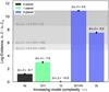 |
Fig. 1 Comparison of the logarithm of the Bayesian evidence (ln 𝒵) for the tested RV models. The evidence difference (Δ ln 𝒵) with the best model, or Bayes Factor (BF), is shown at the top of the bar for each model. In grey are displayed different Δ ln Z from the 2p1c2c model marking the strong evidence against competing models. |
4.2 Search for transits in the TESS light curve
We used the PDCSAP photometry from the two sectors observed by the TESS mission (see Sect. 2.3) on KOBE-1. This instrumentally corrected photometry is flat enough, so we did not need to apply any additional detrending model. Based on the RV analysis from Sect. 4.1, we propagated the expected transit times and their corresponding uncertainties taking into account the uncertainties in both the time of conjunction and the period. The shaded regions in Fig. 3 (first half of sector 17) and Fig. E.9 (the remaining of sector 17 and sector 57) mark the expected location of the propagated transit times for both planets at 68.7% and 95% confidence intervals along both sectors.
A blind application of the tls (Transits Least Square, Heller et al. 2019) to each sector independently suggests a transit with a signal detection efficiency (SDE) of 7.1 in sector 17 while no transit detection in sector 57. Interestingly, the detected signal in sector 17 corresponds to a period of 8.57 d, which is very close to the inferred period for KOBE-1 b from the RV analysis. However, the transit times found (corresponding to BJD − 2 459 800 = 68.66, 77.24, and 85.81) do not match the ephemeris of the RV model, being beyond 3σ. Indeed, the second transit time lays within the downlink gap of the spacecraft and the third one matches a small dimming incompatible in depth with the first one. This, together with the non-detection of transits along sector 57, suggests that the detected transit does not correspond to planet b.
This tls solution is driven by a dimming at time BJD = 2 458 768.66466 d, which is within about 1.0σ from the expected location of the transit for KOBE-1 c according to the RV ephemeris (see Fig. 3). We then explored the possibility that this dimming is caused by the transit of the outer planet instead. This possibility would also explain the absence of transits in sector 57, since the expected time for the transit in this second sector assuming the transit time from sector 17 and the period from the RVs would be at BJD=2459 865.40625252; unfortunately, this lies within the downlink gap of TESS. Consequently, there is only one potential transit for KOBE-1 c among the two available TESS sectors. We caution against claiming a planetary origin of this photometric signal due to the fact that there is only a single transit-like dimming and also because its depth is still at the level of other wiggles in the TESS light curve. In Appendix C, we analyze the dimming to test the transiting KOBE-1 c scenario. We conclude that although these results are promising, there is still no sufficient evidence to claim for a planetary origin of this TESS feature with the data on hand. Additional observations are needed to unveil its origin.
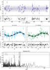 |
Fig. 2 S-BART RV time series (top panel, purple dots) and phase-folded for both planets separately (blue dots in middle-left panel for KOBE-1 b, and green dots in the middle-right panel for KOBE-1 c). The quadratic trend, and the model of the other planet when plotted in phase (middle panels), are subtracted from the RVs. The best model is shown as a solid line, with shaded background regions representing 1- and 2σ confidence intervals. Error bars show the σRV (darker and thicker), and the σjit (lighter and thinner). The residuals of the model are shown in the panels below. Binned measurements in the middle panels are shown as black circles. Bottom: GLS periodogram from the residuals of the model. The grey shaded region indicates the stellar rotational period within 1σ, and its half is shown in dashed red vertical line. False alarm probabilities are indicated with horizontal black lines. |
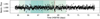 |
Fig. 3 TESS light curves of the first half of sector 17 (before the down-link gap) for KOBE-1. The shaded regions represent the 68.7% (light) and 95% (dark) confidence intervals for the conjunction time of KOBE-1 b (blue) and KOBE-1 c (green) according to the RV analysis in Sect. 4.1. The vertical dotted lines correspond to the median of the expected transit time for each planet, while the vertical dashed red line indicates the location of the detected transit-like feature. The horizontal dashed line corresponds to 1 and the horizontal dotted line corresponds to the depth of a 2 R⊕ planet, for reference. |
5 Discussion
5.1 Confirmation of the planetary nature
At the moment of writing, discussions among the exoplanet community are ongoing with respect to defining an Exoplanet Confirmation Protocol (ECP, Lillo-Box et al., in prep.), aimed at clarifying the minimum requirements for a detected signal to become a confirmed planet. Under the current scheme, this protocol is based on the accomplishment of three generic principles: 1) signal and model significance (first generic principle); 2) demonstrated origin of the signal (second generic principle); and 3) confirming that the signal comes from an object in the planetary-mass domain (third generic principle) to ensure it accomplishes the IAU working definition of extrasolar planets (see Lecavelier des Etangs & Lissauer 2022). The KOBE experiment, as an RV-driven exoplanet search survey, is committed to abide to this protocol. In this section, we summarize the evidence to classify the two signals reported around KOBE-1 as “confirmed planets”.
Significance. Throughout this paper, we show that the RV signals of the two planets, KOBE-1 b and KOBE-1 c, reach a significant level, with the key parameter of the semi-amplitude of the RV converging to values above a 6σ threshold (Kb = 3.75 ± 0.48 m s−1 and Kc = 3.50 ± 0.45 m s−1). In both cases, taking into account the stellar properties derived in Sect. 3, the amplitude of the signals are compatible with them being in the planetary mass domain, corresponding to minimum masses of mb sin ib = 8.80 ± 0.76 M⊕ and mc sin ic = 12.4 ± 1.1 M⊕. Regarding the significance of the model, the log-evidence of the two-planet model is favored over the one-planet hypothesis with respect to the commonly agreed significance threshold (Δ ln 𝒵2p1c2c−1p1c = 7.9). The evidence of these two-planet model against the null-hypothesis is very consistent in time, with a steady increase in the Δ ln 𝒵2p1c2c−0p metric over the course of the observations (see Fig. 4). Additionally, consistency is also seen in the evolution of the Bayesian GLS (BGLS, Mortier et al. 2014; Mortier & Collier Cameron 2017) for both periodicities as new measurements are added (see the stacked BGLS in Fig. 5). In Appendix D, we also show the evolution of the RV semi-amplitudes for both periodicities, demonstrating that they are consistent throughout the four observed seasons. Hence, the signals from both planets satisfy the first generic principle of the ECP.
Origin of the signal. The Gaia renormalized unit weight error (RUWE, which evaluates the behavior of the center of light, see Lindegren et al. 2018) for KOBE-1 is 1.057; hence, Gaia is able to provide a solid astrometric solution to this star, suggesting that no additional sources are present nearby (< 1.4, Lindegren et al. 2018). Moreover, other metrics in Gaia DR3 help rule out long-term systemic RV variability, such as its uncertainty in the median of the epoch or similar criteria (see e.g., Katz et al. 2023) and the fraction of double transits (which evaluates the likelihood of an unseen stellar companion; e.g., Holl et al. 2023). Also, the Gaia DR3 catalog does not include any additional sources within 10 arcsec. From the spectroscopy, the cross-correlation functions obtained by our SHAQ pipeline do not show any additional sharp components that could highlight the presence of a companion blended within the CARMENES fiber aperture. Additionally, the bisector span and FWHM time series do not show correlation with the RVs (see Fig. E.1) that could be attributed to the RV variations being due to another star or a blended binary in a hierarchical triple with KOBE-1. All in all, the RV signal from both planets can be clearly attributed to KOBE-1 and so we are in a position to fulfill the second generic principle of the ECP.
Planetary mass domain. The low minimum masses inferred for both signals imply that for these to be beyond the planetary-mass regime (13 MJup, as defined by the working definition of exoplanet from the IAU), the orbital inclinations must be below 0.12° and 0.17° for KOBE-1 b and KOBE-1 c, respectively.
Assuming no preference for the orbital orientation with respect to our line of sight, the probability of these ranges are 0.13% and 0.19%; alternatively, there is a 99.87% and 99.81% of probability for both planets to be within the planetary-mass domain. These probabilities are larger than the 99.73% threshold to consider a RV-only signal as a confirmed planet, thus both satisfying the third generic principle of the ECP.
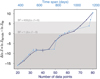 |
Fig. 4 Evolution of the difference between the evidence of the two- planet model and the zero-planet model as a function of the number of data points (dark blue solid line and symbols, corresponding to the lower X-axis) and against the time from the first observation (light blue dotted line and symbols, corresponding to the upper X-axis). The regimes of Δ ln 𝒵 < 6 (or BF = 400) and Δ ln 𝒵 < 0 (BF = 1) are shown as dark and gray shaded regions, respectively. |
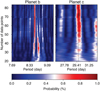 |
Fig. 5 Evolution of the BGLS periodogram as new measurements are added. Top panels show this evolution for KOBE-1 b (left) and KOBE- 1 c (right). Bottom panel shows the color map indicating the probability of the Keplerian origin. |
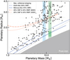 |
Fig. 6 Planetary mass-radius diagram. Vertical regions indicate the minimum mass within 1σ of the planets detected around KOBE-1 (blue for planet b, and green for c). Darker green region shows the 1σ location for KOBE-1 c if we assume it causes the single-TESS transit (solely for illustrative purposes; see more in Sect. 4.2 and Appendix C). Different radius-mass models are shown as identified in the legend to guide the reader on the separated populations (blue lines trace tracks for superEarths and orange lines for sub-Neptunes; Zeng et al. 2019; Aguichine et al. 2021). CMF and WMF refer to the core and water mass fractions, respectively. |
5.2 Warm super-Earths or sub-Neptunes
The minimum masses for both detected planets are compatible either with the super-Earth or sub-Neptune populations. As far as their orbital inclinations are above 35° (KOBE-1 b) and 55° (KOBE-1 c), their absolute masses would be compatible with the current super-Earth population (assuming as a limiting mass that of WASP-84 c with  ). On the other side of the radius. valley (≳1.8 R⊕, Fulton et al. 2017), the sub-Neptune regime is less restrictive, ranging up to 25 Μ⊕.
This degeneracy is shown in the radius-mass diagram of Fig. 6, where the vertical colored lines display the 68.7% confidence interval for the two planets minimum masses. The black dots show the exoplanet population, corresponding to confirmed planets with masses estimated from RVs, and relative errors for both mass and radius below 30 %18 according with the NASA Exoplanet Archive table19 (Akeson et al. 2013). For illustrative reasons, we included four possible interior models using the mr-plotter code20 (Castro-González et al. 2023) that track the sub-Neptune (orange) and super-Earth (blue) populations.
The darker green region in Fig. 6 indicates the KOBE-1 c location assuming that the TESS transit-like dimming corresponds with its transit (see Appendix C, 1.69 ± 0.12 R⊕). Although this is very close to the maximum collisional stripping limit model (Marcus et al. 2010), such a scenario could be feasible. In such a case, KOBE-1 c would be compatible in terms of mass and radius with WASP-84 c (ρ ~ 2.0 ρ⊕) and TOI-1347 b (ρ ~ 1.8 ρ⊕, Polanski et al. 2024), belonging to the densest superEarths, with ρc ~ 2.3 ρ⊕. However, while the ultra-short orbital period of the two known super-Earths (below 1.5 d) can explain their small radius through photo-evaporation, this would not be the case for KOBE-1 c since it is low irradiated by the host star (Sc ~ 3.9 S⊕, in a ~30 d orbital period). Future photometric observations of the target are therefore required to test this hypothesis.
5.3 Sensitivity limits
To measure the sensitivity of the RV dataset to undetected Keplerian signals, we proceeded as in Standing et al. (2022), Standing et al. (2023), and John et al. (2023). For this purpose, we first subtracted the solution from the two-planet model (the highest likelihood posterior sample with eccentricities <0.1) obtained when running kima with Np as a free parameters (see Sect. 4.1 and Table F.6). This sample has periods of Pb = 8.539 d and Pc = 29.625 d, semi-amplitudes of Kb = 3.36 m s−1 and Kc = 3.34 m s−1, and eccentricities of eb = 0.006 and ec = 0.011. To ensure that the residuals do not include any remaining of the signals, we run kima once again with Np as a free parameter. We confirmed that this yielded posterior samples favouring 0 signals.
We then run kima on the residual data yet again following the process described in Standing et al. (2022) out to a maximum period of twice the time span of the data (2000 d). This time, the number of planetary signals was fixed to one (Np = 1). This yielded posterior samples with signals that are compatible with the data, though not formally detected.
In total, more than 400 000 posterior samples were obtained. These samples were then split into period bins, and the 99% upper limit in each bin was calculated. This provided the detection limit which can be found in Fig. 7. Uncertainties on these limits were calculated as in Standing et al. (2023). Signals above the blue detection limit line would have been detected in the initial kima run (checking there were no signals in the residuals). We can see that the red line using only samples with small eccentricities (<0.1) is lower on average than that of the blue line, which is why Standing et al. (2022) warns against the assumption of circular orbits when calculating detection limits. Within the conservative HZ the KOBE-1 dataset is sensitive down to masses of approximately 8.5 M⊕ at an orbital period of ~90–105 d. While, within the optimistic HZ we are sensitive down to masses of approximately 7.6 M⊕ at orbital periods of approximately ~80 d.
5.4 Prospects for further characterization
5.4.1 Gaia astrometry
We computed the astrometric signatures for both KOBE-1 planets by using the stellar and planetary properties from Tables F.5 and F.7. We used the definition from Perryman et al. 2014, with the signature being α = a★/d = (mp/M★) × (ap/d), with the planetary semi-major axis ap in AU, and the system distance d in pc. Hence, we obtained αb = 0.116 ± 0.012 μas and αc = 0.403 ± 0.041 μas. Even these estimated astrometric signatures are upper limits, assuming the most favorable co-planar face-on configuration (sin i ~ 1) and assuming no overestimation in the mass, these signatures are too small even for the most precise astrometric measurements currently available, those published by Gaia in their Data Release 3 (Pourbaix et al. 2022). Since the expected Gaia end-of-mission parallax precision (~10 μas for 9 ⩽ G ⩽ 12, see Gaia Collaboration 2018) is still well above these estimated astrometric signatures, no evidence for the presence of KOBE-1 b and KOBE-1 c is expected from the astrometric technique.
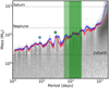 |
Fig. 7 Hexbin plot showing the posterior samples obtained from kima runs on the KOBE-1 RV data with Np fixed to 1. The blue line shows the 99% detection limit line, whereas the red line shows the same line computed on a subset of posterior samples with eccentricity <0.1. The uncertainties on these lines are illustrated by the faded lines of the associated color. The blue and green points represent KOBE-1 b and c, respectively. The extents of the optimistic and conservative HZ for the KOBE-1 system are denoted by the light and dark green shaded regions. |
5.4.2 LIFE direct imaging
Direct imaging is required to characterize non-transiting planets. However, the small angular separation (θb = 2.9 mas and θc = 6.7 mas) and masses of these two planets make them unsuitable for current instruments. For this reason, we used LIFEsim21 (Dannert et al. 2022) to estimate the integration times that would be required to detect both planets with the LIFE mission (Quanz et al. 2022), a project based on nulling interferometry that is aimed at detecting warm worlds in the mid-infrared domain.
We assumed the planets to emit as black bodies, for which we used their equilibrium temperatures collected in Table F.7. In terms of their size, we considered two possible scenarios for each planet (see Sect. 5.2): the super-Earths (SEs) and the miniNeptunes (MNs). For KOBE-1 b we considered Rb,SE = 1.75 R⊕ (Earth-like composition) and Rb,MN = 2.4 R⊕ (20% CMF, and 40% WMF, for Teq,b based on Aguichine et al. 2021 models).
Similarly, for KOBE-1 c, we used Rc,SE = 1.69 R⊕ (Mercury-like composition based on the TESS dimming, see Appendix C) and Rc,MN = 2.5 R⊕ (20% CMF and 40% WMF for Teq,c). We included all the astrophysical noise sources considered by LIFEsim (the stellar leakage, local zodiacal, and exozodiacal light) with a dust level of one zodi. Additionally, we tested the three instrumental scenarios available (optimistic, baseline, and pessimistic) varying the aperture diameter for each of the four- collecting telescopes (3.5 m, 2 m, 1 m) and wavelength-range coverage (3–20 µm, 4–18.5 µm, and 6–17 µm), with the spectral resolution fixed at 20.
Following previous LIFE works (Quanz et al. 2022; Kammerer et al. 2022; Carrión-González et al. 2023), we consider a planet to be detected when the signal-to-noise ratio (S/N) integrated over the wavelength range is above 7. Promisingly, all the simulations result in a detection. For KOBE-1 b the integration times span from 5 min to 13 h, and for KOBE-1 c from 10 min to 44h, for the mini-Neptune and optimistic and superEarth & pessimistic tests, respectively. We include in Table F.9 the integration time for all the studied cases. These results place the KOBE-1 planetary system as an interesting target for the LIFE mission.
6 Conclusions
In this work, we present the exoplanetary system KOBE-1, the first discovery of the KOBE experiment. It consists of two planets with orbital periods of 8.5 d (KOBE-1 b) and 29.7 d (KOBE-1 c). Over three consecutive years, we monitored the quiet star KOBE-1 using the CARMENES spectrograph. These data enabled the detection of the planets with a 7σ significance, which translates into a precise determination of their minimum masses with 11σ significance (mb sin ib = 8.80 ± 0.76 M⊕ and mc sin ic = 12.4 ± 1.1 M⊕). Both planets, with minimum masses below that of Neptune, are consistent with either the super-Earth or mini-Neptune classifications.
We confirmed the planetary nature of KOBE-1 b and KOBE- 1 c based solely on their RV data. This conclusion follows the principles of the ECP (Lillo-Box et al., in prep.), supported by the high significance of the signals, robust Bayesian evidence favoring the planetary scenario over simpler models, and the rejection of alternative non-planetary configurations with a probability above 99.7%.
The outer planet orbits at a moderate distance from the star (0.16071 ± 0.00099 au or a period of 29.7 d), albeit with an insolation about 3.9 times that received by Earth from the Sun and; hence, it is located within the inner edge of the optimistic HZ. Nevertheless, our observational campaign offers a good coverage of this HZ, spanning three full seasons and the beginning of a fourth one, with each lasting around 200 d and with an average of 24 data points per season. A sensitivity analysis using the kima package ruled out the presence of planets with minimum masses above 8.5 M⊕ within the HZ.
In Sect. 4.2, we explored a single dimming event detected by TESS in sector 17 that we cannot attribute to any of the two planets here discovered with the data in hand. Even if none of the KOBE-1 planets transit, we conclude that this system could be fully characterized with future direct imaging space missions. Our analysis shows that the LIFE mission concept would require reasonable integration times to detect both planets: one hour for KOBE-1 b and four hours for KOBE-1 c, assuming a baseline configuration of the instrument and for the extreme scenario, where both planets are super-Earths rather than larger mini-Neptunes.
Data availability
Figures E.2–E.9 from Appendix E and Tables F.3, F.4, F.6, F.8–F.10 from Appendix F are only available in electronic form at https://zenodo.org/records/14511891 and https://zenodo.org//records/14516037. Full version of Tables F.1 and F.2 are available at the CDS via anonymous ftp to cdsarc.cds.unistra.fr (130.79.128.5) or via https://cdsarc.cds.unistra.fr/viz-bin/cat/J/A+A/694/A15.
Acknowledgements
We thank the anonymous referee for their revision of this manuscript that helped to improve its final quality. We acknowledge the huge effort from the Calar Alto observatory personnel in running the KOBE experiment. In particular, Enrique de Guindos and Enrique de Juan for their outstanding work and help on the computing and data access side. We thank Rodrigo Fernando Díaz for the useful discussions on Bayesian statistics. We also thank Carlos Rodrigo Blanco (always in our memories) for his generous work in the development of the KOBE database. This Project has been funded by grants PID2019-107061GB-C61, PID2023-150468NB-I00 and MDM- 2017-0737 by the Spanish Ministry of Science and Innovation/State Agency of Research MCIN/AEI/10.13039/501100011033. J.L.-B. is partially funded by the NextGenerationEU/PRTR grant CNS2023-144309. A.M.S. acknowledges support from the Fundação para a Ciência e a Tecnologia (FCT) through the Fellowship 2020.05387.BD (DOI: 10.54499/2020.05387.BD). Funded/Co-funded by the European Union (ERC, FIERCE, 101052347). Views and opinions expressed are however those of the author(s) only and do not necessarily reflect those of the European Union or the European Research Council. Neither the European Union nor the granting authority can be held responsible for them. This work was supported by FCT – Fundação para a Ciência e a Tecnologia through national funds by these grants: UIDB/04434/2020, UIDP/04434/2020. M.R.S. acknowledges support from the European Space Agency as an ESA Research Fellow. E.M. acknowledges financial support through a “Margarita Salas” postdoctoral fellowship from Universidad Complutense de Madrid (CT18/22), funded by the Spanish Ministerio de Universidades with NextGeneration EU funds. A.A. is supported by NASA’S Interdisciplinary Consortia for Astrobiology Research (NNH19ZDA001N-ICAR) under grant number 80NSSC21K0597. J.C.M. acknowledges financial support from the Spanish Agencia Estatal de Investigación of the Ministerio de Ciencia e Innovación through projects PID2021-125627OB-C31, by “ERDF A way of making Europe”, by the programme Unidad de Excelencia María de Maeztu CEX2020-001058-M. E.D.M. acknowledges the support from FCT through Stimulus FCT contract 2021.01294.CEECIND, and from the Ramón y Cajal grant RyC2022- 035854-I funded by MICIU/AEI/10.13039/50110001103 and by ESF+. A.B. was funded by TED2021-130216A-I00 (MCIN/AEI/10.13039/501100011033 and European Union NextGenerationEU/PRTR). S.C.C.B. acknowledges the support from Fundação para a Ciência e Tecnologia (FCT) in the form of work of work through the Scientific Employment Incentive program (reference 2023.06687.CEECIND). V.A. was supported by Fundação para a Ciência e Tecnologia through national funds and by FEDER through COM-PETE2020 – Programa Operacional Competitividade e Internacionalização by these grants: UIDB/04434/2020; UIDP/04434/2020; 2022.06962.PTDC. S.G.S acknowledges the support from FCT through Investigador FCT contract nr. CEECIND/00826/2018 and POPH/FSE (EC). E.N. acknowledges the support by the DFG Research Unit FOR2544 “Blue Planets around Red Stars”. The project leading to this publication has received funding from the Excellence Initiative of Aix-Marseille University – A*Midex, a French “Investissements d’Avenir programme” AMX-19-IET-013. This work was supported by the “Programme National de Planétologie” (PNP) of CNRS/INSU co-funded by CNES. The KOBE archive and the VOSA code are both developed under the Spanish Virtual Observatory (svo.cab.inta-csic.es), project funded by MCIN/AEI/10.13039/501100011033/ through grant PID2020-112949GB-I00. This research made use of astropy, (a community-developed core Python package for Astronomy, Astropy Collaboration 2013, 2018), SciPy (Virtanen et al. 2020), matplotlib (a Python library for publication quality graphics Hunter 2007), astroML (Vanderplas et al. 2012), numpy (Harris et al. 2020), and dfitspy (Thomas 2019). This research has made use of NASA’s Astrophysics Data System (ADS) Bibliographic Services, the SIMBAD database operated at CDS, the Exoplanet Follow-up Observation Program (ExoFOP; DOI: 10.26134/ExoFOP5) website, and the NASA Exoplanet Archive, the latter two are operated by the California Institute of Technology under contract with the National Aeronautics and Space Administration under the Exoplanet Exploration Program. This material is based upon work supported by NASA’S Interdisciplinary Consortia for Astrobiology Research (NNH19ZDA001N-ICAR) under award number 19-ICAR19_2-0041.
Appendix A Comparison of the RV extraction by different pipelines
Silva et al. (2022) presented the S-BART pipeline and compared the behavior of different RV extraction methods (CCF, classical template matching, and their semi-Bayesian template-matching approximation) with the stellar spectral-type (M-, K-, and G-dwarf stars). They found that S-BART provides a better precision (i.e., lower σ-RV) than CCF-based pipelines for the three studied stellar spectral types. Besides, the S-BART precision as compared with those from classical template matching improves when going to earlier types than M-dwarfs (for K- and more notably for G-type stars, see Fig. 14 from their publication).
In Fig. A.1 we compare the distributions of the RVs (top) and their uncertainties (bottom) extracted by the three pipelines used in this work (S-BART, serval, and SHAQ) for KOBE-1 (left), the six KOBE standard stars (middle), and the NZPs (right). KOBE-1 is a K7 V star, a domain where classical template-matching algorithms (e.g., serval) reach high precisions, being compatible with those from S-BART, and significantly better than CCF (e.g., SHAQ) as can be seen in the bottom left panel of Fig. A.1. Nonetheless, the spectral type of the standard stars used in KOBE range from G6 V to KO V. Consequently, serval is not optimized to obtain the RVs of these six targets and, as a result, the RMS of the NZPs obtained with serval double those of S-BART and have a 39% lower precision (see middle and right columns from Fig. A.1). As the serval NZP correction is not optimal, if correcting with its NZPs there is a high dispersion of the final KOBE-1 RVs (see top left panel from Fig. A.1) that can hide the planetary signals (8.5 and 29.7d).
As S-BART is the only pipeline extracting high quality RV measurements from the standards, we corrected the CARMENES KOBE-1 RVs from the three pipelines (S-BART, serval, and SHAQ) with S-BART NZPs. In Fig. A.2 we show the GLS periodograms for these three time series, where the planet b periodicity (8.5 d) is present for all of them, and the outer signal (29.7 d) is only missed by SHAQ probably as a result of its higher σRV (see again bottom left panel in Fig. A.1). Therefore, we demonstrated that three different methodologies recover compatible time series.
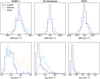 |
Fig. A.1 RV distributions (top) and their associated uncertainties (bottom) for each pipeline (color code as shown in the legend of the top left panel). Columns correspond to KOBE-1 (left), the six KOBE standards (middle), and the NZPs (left). |
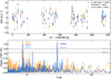 |
Fig. A.2 Comparison of data from different pipelines. Top: CARMENES RV time series extracted by S-BART, serval and SHAQ pipelines corrected with S-BART NZPs in all cases. Bottom: Periodogram for the datasets shown above. The horizontal black lines indicate the different false alarm probabilities. |
Appendix B The 29.7-days periodicity
Given that the period of the external signal  is close to the synodic period of the Moon (29.53 d), we checked the Moon separation and illumination of our observations. As detailed in Sect. 2, we found that nine data points are potentially contaminated by the Moon illumination (including angular separations < 80°, Moon illumination > 40% and BERV < 21 km s−1), hence we removed them from our dataset. In Fig. B.1, we show the periodogram of the complete dataset (blue line), the cleaned sample after removing the Moon-contaminated datapoints (green line) and the contaminated data points (red line). As shown, the periodicity at 29.7 d remains in the cleaned sample and it is not present in the contaminated sample. The fact that the significance of the 29.7 d signals decreases when removing this dataset is attributed to the fact that i) we are removing about 10% of the data points, and ii) that the phases corresponding to the contaminated observations cluster in a region where there are few other uncontaminated observations.
Another possible origin of this signal, also related to the synodic periodicity, is that the BERV correction is wrongly accounting for the Moon motion. If this would be the case, we would see similar periodicities in the RVs of other KOBE targets (whose BERV are calculated using the same procedure). This is not the case, and indeed, the only KOBE target showing a periodicity close to this synodic period is KOBE-1.
Additionally, the maximum impact that the Moon contamination could have on KOBE-1 RVs, based on its magnitude (V ~ 10 mag) and spectral type (K7 V), is below 0.3 m s−1 as estimated in Cunha et al. (2013) (see their Fig. 5), which is negligible for the CARMENES precision (> 1.5 m s−1). Such an upper limit for the induced error is eleven times weaker than the signal found in this work (Kc = 3.50 ± 0.45 m s−1). All in all, our data and the analysis presented in this section supports that the origin of this 29.7 d signal is different from the synodic period of the Moon.
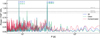 |
Fig. B.1 GLS periodogram of the full sample of RVs obtained for KOBE-1 (blue line), the sub-sample of data points after excluding the possibly Moon-contaminated observations (green line) and the sub-sample of the affected data points (red line). The three false alarm probability level of 10%, 5% and 1% are shown as black horizontal lines. |
Appendix C TESS-CARMENES compatibility for a transiting KOBE-1 c
We analyzed the dimming found in Sect. 4.2 assuming its origin from KOBE-1 c to extract the compatible planetary parameters. We used the batman22 code (Kreidberg 2015) to produce the planet transit model. Since we aimed at checking the compatibility of the transit signal with the RV solution for KOBE-1 c, we used a tight Gaussian prior on its orbital period based on the marginalized posterior distribution from Sect. 4.1, and a uniform prior on the time of mid-transit including the whole first part of sector 17. We then imposed a uniform prior on the inclination allowing for large values not inducing transits, and a uniform prior on the planet radius of 𝒰(0, 10) R⊕. We estimated the quadratic limb-darkening coefficients using the limb-darkening23 code from Espinoza & Jordán (2015) using the stellar parameters derived in Sect. 3, and used a Gaussian prior around these values with a 10% width. We also used the stellar radius as a parameter with a Gaussian prior based on the results from Sect. 3. Finally, we added an offset parameter for the light curve and a σjit term with sufficiently broad priors. All these priors are specified in Table F.10. We sampled the parameter space using emcee, with four times as many walkers as parameters and 50000 steps per walker with the subsequent second phase as done in the RV analysis (see Sect. 4.1). This analysis resulted in the convergence of the chains towards the transit detected in this sector despite using a conservative uniform prior on the time of conjunction.
The solution converged to a planetary transit with a radius of 1.69 ± 0.12 R⊕ and an orbital inclination of  degrees (corresponding to an impact parameter of
  ), see Fig. C.1. The transit duration of
  hours is within the expectations for a period like the one from KOBE-1 c without requiring a grazing configuration. The median and 68.7% confidence intervals extracted from the marginalized posterior distributions of the inferred parameters, together with other derived parameters are shown in Table F.10.
By performing a joint analysis including the RVs and the TESS light curve, we further tested the compatibility of the signals. This time, we set the priors on the time of conjunction and period of the two-planet model as uniform in a wide range in order to neither bias the final result nor force the transit to be attributed to any of the RV-detected planets. We set the same period priors as for the RV-standalone analysis in Sect. 4.1 and the priors on the planet and stellar properties as in Sect. 4.2. We run a long 100000-step chain with a large number of walkers (10 times the number of free parameters) and sample the posterior distribution of the parameters using emcee.
By the end of the run, none of the chains ended up in a configuration that would produce a transiting signal. However, the periods are well defined and converged to those from planets b and c. Only 0.3% of the samples provided an impact parameter compatible with a transiting signal (b < 1 + Rp/R★). All of them correspond to periods from KOBE-1 c. Those samples correspond to times of conjunction that would make the TESS observations miss the transit. Hence, the joint MCMC analysis definitively suggests that the current data do not prefer the transiting hypothesis for KOBE-1 c.
We suggest several possible explanations for this result. One option is that the transiting signal corresponds to instrumental systematics or stellar noise, as despite being the deepest signal in the data, it is still compatible with the amplitude of other features in other parts of the light curve. Given that only one of such signals is observable in the TESS dataset, we have no further information to test this scenario. Second, even if the feature actually corresponds to a transit of KOBE-1 c, there is some discrepancy at the 1.0σ level between the expected time of conjunction from the RV-standalone analysis and the location of the feature. This tension, together with the shallow and lonely feature, implies that the MCMC prefers to better model the RV data points than finding a compromise between the RVs and the potential transit signal, thus converging to non-transiting configurations. It might be possible that there are relevant transit timing variations accounting for that time discrepancy in case that KOBE-1 c forms part of a resonant chain. Given this analysis, we remain cautious and do not claim that the detected signal is due to a transiting planet in the system. We note that TESS revisits this target in October 2024, during a period when KOBE-1 c is expected to transit.
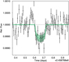 |
Fig. C.1 Transit modeling of the feature detected in the TESS data from sector 17 that may be attributed to KOBE-1 c. The black symbols show the TESS 2-min cadence data from this sector. The green solid line corresponds to the median model from Appendix C and the shaded region to models within the 68.7% confidence interval. |
Appendix D Evolution of the Keplerian signals
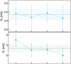 |
Fig. D.1 RV semi-amplitude evolution with the epoch for the signal induced by KOBE-1 b (top) and KOBE-1 c (bottom). Dotted horizontal line represent the mean of the RV semi-amplitude obtained when fitting all epochs with its 1σ shown as a colored shaded region. |
We studied the evolution of the RV semi-amplitudes of the two detected Keplerian signals as an additional test for their consistency. We first modeled the complete RV time series using the quadratic trend and the two Keplerians through the least-square method implemented in the DACE24 web (Delisle et al. 2016). We note that the solution found from this method is compatible with the Bayesian approaches from Sect. 4.1, but for this test we opted for a computationally cheaper analysis. We then split our dataset into four different chucks corresponding to the four visibility time spans from 2021 to 2024. These chunks contain individually an average of 20 data points per chunk. We then model each chunk separately with only the two RV semi-amplitudes as free parameters and fixing all the remaining orbital parameters from the previous solution. We show the evolution of the semi-amplitudes in Fig. D.1.
Signals induced by stellar activity are known to be unstable with time, hence varying both their phase and amplitude (e.g., Mortier & Collier Cameron 2017). This is not the case for any of the two signals found. In Fig. 5 we demonstrated that the signals are significant and their periodicities are stable with the number of measurements. In this appendix, we found that both signals are constant through the time span with results compatible for all epochs within their uncertainties. Therefore, the RV signatures cannot be related with activity and are more likely induced by planetary companions.
Appendix E Additional figures
Figures from E.2 to E.9 can be accessed at Zenodo through https://zenodo.org/records/14511891.
Appendix F Additional tables
Tables F.3, F.4, F.6, F.8 - F.10 can be accessed at Zenodo through https://zenodo.org/records/14516037.
Spectroscopic indicators from the CARMENES time series.
CARMENES RV measurements extracted with sBART and the correspondingly applied nightly zero points and drifts.
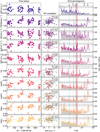 |
Fig. E.1 CARMENES data. Left: Time series for the S-BART RVs and the spectroscopic activity indicators. The grey line shows a quadratic trend fit. Center: Activity indicator and RV correlation, with a linear fit shown in dashed blue line, and the correlation coefficients (R from Pearson, and ρ from Spearman) indicated in the grey box. Right: GLS periodogram to the time series of the same row. The grey line corresponds to the non-detrended time series, while colored lines correspond to the same dataset after subtracting the fitted quadratic function. Vertical lines indicate the periodicities of the planets (blue and green), the rotational period (red region, see Sect. 3.2) and its half (dashed red line), and the duration of the year and its half (dashed grey lines). Horizontal lines show different false alarm probabilities as indicated in the top panel. |
General and dynamical properties of KOBE-1.
Prior and posterior distributions for the best RV model (2p1c2c), with inferred planetary properties.
References
- Aguichine, A., Mousis, O., Deleuil, M., & Marcq, E. 2021, ApJ, 914, 84 [NASA ADS] [CrossRef] [Google Scholar]
- Akeson, R. L., Chen, X., Ciardi, D., et al. 2013, PASP, 125, 989 [Google Scholar]
- Allard, F., Homeier, D., & Freytag, B. 2012, Philos. Trans. Roy. Soc. Lond. Ser. A, 370, 2765 [NASA ADS] [Google Scholar]
- Aller, A., Lillo-Box, J., Jones, D., Miranda, L. F., & Barceló Forteza, S. 2020, A&A, 635, A128 [NASA ADS] [CrossRef] [EDP Sciences] [Google Scholar]
- Aller, A., Lillo-Box, J., & Jones, D. 2024, A&A, 690, A190 [NASA ADS] [CrossRef] [EDP Sciences] [Google Scholar]
- Ambikasaran, S., Foreman-Mackey, D., Greengard, L., Hogg, D. W., & O’Neil, M. 2015, IEEE Trans. Pattern Anal. Mach. Intell., 38, 252 [Google Scholar]
- Arney, G. N. 2019, ApJ, 873, L7 [NASA ADS] [CrossRef] [Google Scholar]
- Astropy Collaboration (Robitaille, T. P., et al.) 2013, A&A, 558, A33 [NASA ADS] [CrossRef] [EDP Sciences] [Google Scholar]
- Astropy Collaboration (Price-Whelan, A. M., et al.) 2018, AJ, 156, 123 [Google Scholar]
- Baraffe, I., Chabrier, G., Allard, F., & Hauschildt, P. H. 1998, A&A, 337, 403 [Google Scholar]
- Baranne, A., Queloz, D., Mayor, M., et al. 1996, A&AS, 119, 373 [NASA ADS] [CrossRef] [EDP Sciences] [Google Scholar]
- Bauer, F. F., Zechmeister, M., & Reiners, A. 2015, A&A, 581, A117 [NASA ADS] [CrossRef] [EDP Sciences] [Google Scholar]
- Bayo, A., Rodrigo, C., Barrado y Navascués, D., et al. 2008, A&A, 492, 277 [NASA ADS] [CrossRef] [EDP Sciences] [Google Scholar]
- Beard, C., Robertson, P., Kanodia, S., et al. 2022, ApJ, 936, 55 [NASA ADS] [CrossRef] [Google Scholar]
- Bonfils, X., Forveille, T., Delfosse, X., et al. 2005, A&A, 443, L15 [NASA ADS] [CrossRef] [EDP Sciences] [Google Scholar]
- Bonomo, A. S., Dumusque, X., Massa, A., et al. 2023, A&A, 677, A33 [NASA ADS] [CrossRef] [EDP Sciences] [Google Scholar]
- Borucki, W. J., Koch, D., Basri, G., et al. 2010, Science, 327, 977 [Google Scholar]
- Brewer, B. J., Pártay, L. B., & Csányi, G. 2010, DNEST: Diffusive Nested Sampling, Astrophysics Source Code Library [record ascl:1010.029] [Google Scholar]
- Briggs, G. 2000, Meteoritics Planet. Sci., 35, 892 [CrossRef] [Google Scholar]
- Brown, E. L., Jeffers, S. V., Marsden, S. C., et al. 2022, MNRAS, 514, 4300 [CrossRef] [Google Scholar]
- Carrión-González, Ó., Kammerer, J., Angerhausen, D., et al. 2023, A&A, 678, A96 [NASA ADS] [CrossRef] [EDP Sciences] [Google Scholar]
- Castro-González, A., Díez Alonso, E., Menéndez Blanco, J., et al. 2022, MNRAS, 509, 1075 [Google Scholar]
- Castro-González, A., Demangeon, O. D. S., Lillo-Box, J., et al. 2023, A&A, 675, A52 [NASA ADS] [CrossRef] [EDP Sciences] [Google Scholar]
- Castro-González, A., Lillo-Box, J., Armstrong, D. J., et al. 2024, A&A, 691, A233 [NASA ADS] [CrossRef] [EDP Sciences] [Google Scholar]
- Cifuentes, C., Caballero, J. A., Cortés-Contreras, M., et al. 2020, A&A, 642, A115 [NASA ADS] [CrossRef] [EDP Sciences] [Google Scholar]
- Cifuentes, C., Caballero, J. A., González-Payo, J., et al. 2024, arXiv e-prints [arXiv:2412.12264] [Google Scholar]
- Cosentino, R., Lovis, C., Pepe, F., et al. 2014, SPIE Conf. Ser., 9147, 8 [Google Scholar]
- Cunha, D., Figueira, P., Santos, N. C., Lovis, C., & Boué, G. 2013, A&A, 550, A75 [NASA ADS] [CrossRef] [EDP Sciences] [Google Scholar]
- Cuntz, M., & Guinan, E. F. 2016, ApJ, 827, 79 [NASA ADS] [CrossRef] [Google Scholar]
- Cutri, R. M., Skrutskie, M. F., van Dyk, S., et al. 2003, VizieR Online Data Catalog: 2MASS All-Sky Catalog of Point Sources (Cutri+ 2003), VizieR On-line Data Catalog: II/246 [Google Scholar]
- Dannert, F. A., Ottiger, M., Quanz, S. P., et al. 2022, A&A, 664, A22 [NASA ADS] [CrossRef] [EDP Sciences] [Google Scholar]
- Delisle, J. B., Ségransan, D., Buchschacher, N., & Alesina, F. 2016, A&A, 590, A134 [NASA ADS] [CrossRef] [EDP Sciences] [Google Scholar]
- Díaz, R. F., Ségransan, D., Udry, S., et al. 2016, A&A, 585, A134 [Google Scholar]
- Dumusque, X., Borsa, F., Damasso, M., et al. 2017, A&A, 598, A133 [NASA ADS] [CrossRef] [EDP Sciences] [Google Scholar]
- Eastman, J., Gaudi, B. S., & Agol, E. 2013, PASP, 125, 83 [Google Scholar]
- ESA, ed. 1997, ESA Special Publication, 1200, The HIPPARCOS and TYCHO Catalogues. Astrometric and photometric star catalogues derived from the ESA HIPPARCOS Space Astrometry Mission [Google Scholar]
- Espinoza, N., & Jordán, A. 2015, MNRAS, 450, 1879 [Google Scholar]
- Faria, J. P., Santos, N. C., Figueira, P., & Brewer, B. J. 2018, J. Open Source Softw., 3, 487 [NASA ADS] [CrossRef] [Google Scholar]
- Faria, J. P., Suárez Mascareño, A., Figueira, P., et al. 2022, A&A, 658, A115 [NASA ADS] [CrossRef] [EDP Sciences] [Google Scholar]
- Foreman-Mackey, D., Hogg, D. W., Lang, D., & Goodman, J. 2013, PASP, 125, 306 [Google Scholar]
- Fulton, B. J., Petigura, E. A., Howard, A. W., et al. 2017, AJ, 154, 109 [Google Scholar]
- Fulton, B. J., Petigura, E. A., Blunt, S., & Sinukoff, E. 2018, PASP, 130, 044504 [Google Scholar]
- Gaia Collaboration (Brown, A. G. A., et al.) 2018, A&A, 616, A1 [NASA ADS] [CrossRef] [EDP Sciences] [Google Scholar]
- Gaidos, E., Mann, A. W., Lépine, S., et al. 2014, MNRAS, 443, 2561 [Google Scholar]
- Georgieva, I. Y., Persson, C. M., Goffo, E., et al. 2023, A&A, 674, A117 [NASA ADS] [CrossRef] [EDP Sciences] [Google Scholar]
- Gliese, W. 1969, Veroeffentlich. Astron. Rechen-Inst. Heidelberg, 22, 1 [Google Scholar]
- Gomes da Silva, J., Figueira, P., Santos, N., & Faria, J. 2018, J. Open Source Softw., 3, 667 [Google Scholar]
- Gray, R. O., Corbally, C. J., Garrison, R. F., McFadden, M. T., & Robinson, P. E. 2003, AJ, 126, 2048 [Google Scholar]
- Gullikson, K. 2014, TelFit: Fitting the telluric absorption spectrum, Astrophysics Source Code Library [record ascl:1405.002] [Google Scholar]
- Hacker, A., Díaz, R. F., Armstrong, D. J., et al. 2024, MNRAS, 532, 1612 [NASA ADS] [CrossRef] [Google Scholar]
- Harris, C. R., Millman, K. J., van der Walt, S. J., et al. 2020, Nature, 585, 357 [NASA ADS] [CrossRef] [Google Scholar]
- Haywood, R. D., Collier Cameron, A., Queloz, D., et al. 2014, MNRAS, 443, 2517 [Google Scholar]
- Heller, R., Rodenbeck, K., & Hippke, M. 2019, A&A, 625, A31 [NASA ADS] [CrossRef] [EDP Sciences] [Google Scholar]
- Holl, B., Fabricius, C., Portell, J., et al. 2023, A&A, 674, A25 [NASA ADS] [CrossRef] [EDP Sciences] [Google Scholar]
- Hubbard, G. S., Naderi, F. M., & Garvin, J. B. 2002, Acta Astronaut, 51, 337 [NASA ADS] [CrossRef] [Google Scholar]
- Hunter, J. D. 2007, Comput. Sci. Eng., 9, 90 [NASA ADS] [CrossRef] [Google Scholar]
- Isaacson, H., & Fischer, D. 2010, ApJ, 725, 875 [Google Scholar]
- Jenkins, J. M., Twicken, J. D., McCauliff, S., et al. 2016, SPIE Conf. Ser., 9913, 99133E [Google Scholar]
- John, A. A., Collier Cameron, A., Faria, J. P., et al. 2023, MNRAS, 525, 1687 [Google Scholar]
- Kammerer, J., Quanz, S. P., Dannert, F., & LIFE Collaboration 2022, A&A, 668, A52 [NASA ADS] [CrossRef] [EDP Sciences] [Google Scholar]
- Kass, R. E., & Raftery, A. E. 1995, J. Am. Statist. Assoc., 90, 773 [CrossRef] [Google Scholar]
- Kasting, J. F., Whitmire, D. P., & Reynolds, R. T. 1993, Icarus, 101, 108 [Google Scholar]
- Katz, D., Sartoretti, P., Guerrier, A., et al. 2023, A&A, 674, A5 [NASA ADS] [CrossRef] [EDP Sciences] [Google Scholar]
- Koen, C., Kilkenny, D., van Wyk, F., & Marang, F. 2010, MNRAS, 403, 1949 [Google Scholar]
- Kopparapu, R. K., Ramirez, R., Kasting, J. F., et al. 2013, ApJ, 765, 131 [NASA ADS] [CrossRef] [Google Scholar]
- Kreidberg, L. 2015, PASP, 127, 1161 [Google Scholar]
- Kunimoto, M., & Matthews, J. M. 2020, AJ, 159, 248 [NASA ADS] [CrossRef] [Google Scholar]
- Lafarga, M., Ribas, I., Lovis, C., et al. 2020, A&A, 636, A36 [NASA ADS] [CrossRef] [EDP Sciences] [Google Scholar]
- Lecavelier des Etangs, A., & Lissauer, J. J. 2022, New Astron. Rev., 94, 101641 [CrossRef] [Google Scholar]
- Lightkurve Collaboration (Cardoso, J. V. d. M., et al.) 2018, Lightkurve: Kepler and TESS time series analysis in Python, Astrophysics Source Code Library [record ascl:1812.013] [Google Scholar]
- Lillo-Box, J., Figueira, P., Leleu, A., et al. 2020, A&A, 642, A121 [NASA ADS] [CrossRef] [EDP Sciences] [Google Scholar]
- Lillo-Box, J., Faria, J. P., Suárez Mascareño, A., et al. 2021, A&A, 654, A60 [NASA ADS] [CrossRef] [EDP Sciences] [Google Scholar]
- Lillo-Box, J., Santos, N. C., Santerne, A., et al. 2022, A&A, 667, A102 [NASA ADS] [CrossRef] [EDP Sciences] [Google Scholar]
- Lindegren, L., Hernández, J., Bombrun, A., et al. 2018, A&A, 616, A2 [NASA ADS] [CrossRef] [EDP Sciences] [Google Scholar]
- Marcus, R. A., Sasselov, D., Hernquist, L., & Stewart, S. T. 2010, ApJ, 712, L73 [Google Scholar]
- Marfil, E., Tabernero, H. M., Montes, D., et al. 2021, A&A, 656, A162 [NASA ADS] [CrossRef] [EDP Sciences] [Google Scholar]
- Martínez-Arnáiz, R., Maldonado, J., Montes, D., Eiroa, C., & Montesinos, B. 2010, A&A, 520, A79 [NASA ADS] [CrossRef] [EDP Sciences] [Google Scholar]
- Montes, D., López-Santiago, J., Fernández-Figueroa, M. J., & Gálvez, M. C. 2001, A&A, 379, 976 [CrossRef] [EDP Sciences] [Google Scholar]
- Mortier, A., & Collier Cameron, A. 2017, A&A, 601, A110 [NASA ADS] [CrossRef] [EDP Sciences] [Google Scholar]
- Mortier, A., Sousa, S. G., Adibekyan, V. Z., Brandão, I. M., & Santos, N. C. 2014, A&A, 572, A95 [NASA ADS] [CrossRef] [EDP Sciences] [Google Scholar]
- Noyes, R. W., Weiss, N. O., & Vaughan, A. H. 1984, ApJ, 287, 769 [Google Scholar]
- Osborne, H. L. M., Van Eylen, V., Goffo, E., et al. 2024, MNRAS, 527, 11138 [Google Scholar]
- Palethorpe, L., John, A. A., Mortier, A., et al. 2024, MNRAS, 529, 3323 [NASA ADS] [Google Scholar]
- Passegger, V. M., Suárez Mascareño, A., Allart, R., et al. 2024, A&A, 684, A22 [NASA ADS] [CrossRef] [EDP Sciences] [Google Scholar]
- Pepe, F., Lovis, C., Ségransan, D., et al. 2011, A&A, 534, A58 [CrossRef] [EDP Sciences] [Google Scholar]
- Pepe, F., Cristiani, S., Rebolo, R., et al. 2021, A&A, 645, A96 [NASA ADS] [CrossRef] [EDP Sciences] [Google Scholar]
- Perrakis, K., Ntzoufras, I., & Tsionas, E. G. 2014, Computat. Statist. Data Anal., 77, 54 [CrossRef] [Google Scholar]
- Perryman, M., Hartman, J., Bakos, G. Á., & Lindegren, L. 2014, ApJ, 797, 14 [Google Scholar]
- Polanski, A. S., Lubin, J., Beard, C., et al. 2024, ApJS, 272, 32 [NASA ADS] [CrossRef] [Google Scholar]
- Poretti, E., Boccato, C., Claudi, R., et al. 2016, Mem. Soc. Astron. Italiana, 87, 141 [NASA ADS] [Google Scholar]
- Pourbaix, D., Arenou, F., Gavras, P., et al. 2022, Gaia DR3 Documentation, Chapter 7: Non-single stars, Gaia DR3 documentation, European Space Agency; Gaia Data Processing and Analysis Consortium. Online at https://gea.esac.esa.int/archive/documentation/GDR3/index.html, 7 [Google Scholar]
- Quanz, S. P., Ottiger, M., Fontanet, E., et al. 2022, A&A, 664, A21 [NASA ADS] [CrossRef] [EDP Sciences] [Google Scholar]
- Quirrenbach, A., Amado, P. J., Caballero, J. A., et al. 2014, SPIE Conf. Ser., 9147, 1 [Google Scholar]
- Rajpaul, V., Aigrain, S., Osborne, M. A., Reece, S., & Roberts, S. 2015, MNRAS, 452, 2269 [Google Scholar]
- Reid, I. N., Hawley, S. L., & Gizis, J. E. 1995, AJ, 110, 1838 [Google Scholar]
- Reiners, A., Zechmeister, M., Caballero, J. A., et al. 2018, A&A, 612, A49 [NASA ADS] [CrossRef] [EDP Sciences] [Google Scholar]
- Ribas, I., Reiners, A., Zechmeister, M., et al. 2023, A&A, 670, A139 [NASA ADS] [CrossRef] [EDP Sciences] [Google Scholar]
- Ricker, G. R., Winn, J. N., Vanderspek, R., et al. 2014, SPIE Conf. Ser., 9143, 20 [Google Scholar]
- Rutten, R. G. M. 1984, A&A, 130, 353 [NASA ADS] [Google Scholar]
- Schweitzer, A., Passegger, V. M., Cifuentes, C., et al. 2019, A&A, 625, A68 [NASA ADS] [CrossRef] [EDP Sciences] [Google Scholar]
- Shappee, B. J., Prieto, J. L., Grupe, D., et al. 2014, ApJ, 788, 48 [Google Scholar]
- Silva, A. M., Faria, J. P., Santos, N. C., et al. 2022, A&A, 663, A143 [NASA ADS] [CrossRef] [EDP Sciences] [Google Scholar]
- Standing, M. R., Triaud, A. H. M. J., Faria, J. P., et al. 2022, MNRAS, 511, 3571 [NASA ADS] [CrossRef] [Google Scholar]
- Standing, M. R., Sairam, L., Martin, D. V., et al. 2023, Nat. Astron., 7, 702 [NASA ADS] [CrossRef] [Google Scholar]
- Stassun, K. G., Oelkers, R. J., Paegert, M., et al. 2019, AJ, 158, 138 [Google Scholar]
- Suárez Mascareño, A., Rebolo, R., & González Hernández, J. I. 2016, A&A, 595, A12 [Google Scholar]
- Suárez Mascareño, A., Rebolo, R., González Hernández, J. I., & Esposito, M. 2017, MNRAS, 468, 4772 [Google Scholar]
- Suárez Mascareño, A., Passegger, V. M., González Hernández, J. I., et al. 2024, A&A, 685, A56 [NASA ADS] [CrossRef] [EDP Sciences] [Google Scholar]
- Tabernero, H. M., Marfil, E., Montes, D., & González Hernández, J. I. 2022, A&A, 657, A66 [NASA ADS] [CrossRef] [EDP Sciences] [Google Scholar]
- Thomas, R. 2019, dfitspy: A dfits/fitsort implementation in Python, Astrophysics Source Code Library [record ascl:1904.017] [Google Scholar]
- Trifonov, T., Kürster, M., Zechmeister, M., et al. 2018, A&A, 609, A117 [NASA ADS] [CrossRef] [EDP Sciences] [Google Scholar]
- Udry, S., Dumusque, X., Lovis, C., et al. 2019, A&A, 622, A37 [NASA ADS] [CrossRef] [EDP Sciences] [Google Scholar]
- Vanderplas, J., Connolly, A., Ivezic, Ž., & Gray, A. 2012, in Conference on Intelligent Data Understanding (CIDU), 47 [CrossRef] [Google Scholar]
- Virtanen, P., Gommers, R., Oliphant, T. E., et al. 2020, Nat. Methods, 17, 261 [Google Scholar]
- Winecki, D., & Kochanek, C. S. 2024, ApJ, 971, 61 [NASA ADS] [CrossRef] [Google Scholar]
- Zechmeister, M., & Kürster, M. 2009, A&A, 496, 577 [CrossRef] [EDP Sciences] [Google Scholar]
- Zechmeister, M., Reiners, A., Amado, P. J., et al. 2018, A&A, 609, A12 [NASA ADS] [CrossRef] [EDP Sciences] [Google Scholar]
- Zechmeister, M., Anglada-Escudé, G., & Reiners, A. 2014, A&A, 561, A59 [NASA ADS] [CrossRef] [EDP Sciences] [Google Scholar]
- Zeng, L., Jacobsen, S. B., Sasselov, D. D., et al. 2019, PNAS, 116, 9723 [Google Scholar]
See, for instance, the Follow the water premise of NASA (Briggs 2000; Hubbard et al. 2002).
Available at https://github.com/iastro-pt/sBART
Available at https://github.com/kgullikson88/Telluric-Fitter
Available at www.github.com/mzechmeister/serval
Available at https://lightkurve.github.io/lightkurve/
Available at https://github.com/jlillo/tpfplotter
Available at https://github.com/castro-gzlz/tess-cont
Available at https://github.com/dmontesg/SteParKin
Available at https://www.kima.science/docs/
Available at https://radvel.readthedocs.io/en/latest/
Available at https://emcee.readthedocs.io/en/stable/
Available at https://github.com/exord/bayev/tree/master
Available at https://george.readthedocs.io/en/latest/
We discarded the planets HD 63433 b and Kepler-107 c since they are placed in the dense super-Earth domain but their mass estimations are not reliable according with their publications (Polanski et al. 2024; Bonomo et al. 2023).
Available at https://github.com/castro- gzlz/mr-plotter/tree/main
Available at https://lifesim.readthedocs.io/en/latest/index.html
Available at https://github.com/lkreidberg/batman?tab=readme-ov-file
Available at https://github.com/nespinoza/limb-darkening
All Tables
CARMENES RV measurements extracted with sBART and the correspondingly applied nightly zero points and drifts.
Prior and posterior distributions for the best RV model (2p1c2c), with inferred planetary properties.
All Figures
|
Fig. 1 Comparison of the logarithm of the Bayesian evidence (ln 𝒵) for the tested RV models. The evidence difference (Δ ln 𝒵) with the best model, or Bayes Factor (BF), is shown at the top of the bar for each model. In grey are displayed different Δ ln Z from the 2p1c2c model marking the strong evidence against competing models. |
| In the text | |
|
Fig. 2 S-BART RV time series (top panel, purple dots) and phase-folded for both planets separately (blue dots in middle-left panel for KOBE-1 b, and green dots in the middle-right panel for KOBE-1 c). The quadratic trend, and the model of the other planet when plotted in phase (middle panels), are subtracted from the RVs. The best model is shown as a solid line, with shaded background regions representing 1- and 2σ confidence intervals. Error bars show the σRV (darker and thicker), and the σjit (lighter and thinner). The residuals of the model are shown in the panels below. Binned measurements in the middle panels are shown as black circles. Bottom: GLS periodogram from the residuals of the model. The grey shaded region indicates the stellar rotational period within 1σ, and its half is shown in dashed red vertical line. False alarm probabilities are indicated with horizontal black lines. |
| In the text | |
|
Fig. 3 TESS light curves of the first half of sector 17 (before the down-link gap) for KOBE-1. The shaded regions represent the 68.7% (light) and 95% (dark) confidence intervals for the conjunction time of KOBE-1 b (blue) and KOBE-1 c (green) according to the RV analysis in Sect. 4.1. The vertical dotted lines correspond to the median of the expected transit time for each planet, while the vertical dashed red line indicates the location of the detected transit-like feature. The horizontal dashed line corresponds to 1 and the horizontal dotted line corresponds to the depth of a 2 R⊕ planet, for reference. |
| In the text | |
|
Fig. 4 Evolution of the difference between the evidence of the two- planet model and the zero-planet model as a function of the number of data points (dark blue solid line and symbols, corresponding to the lower X-axis) and against the time from the first observation (light blue dotted line and symbols, corresponding to the upper X-axis). The regimes of Δ ln 𝒵 < 6 (or BF = 400) and Δ ln 𝒵 < 0 (BF = 1) are shown as dark and gray shaded regions, respectively. |
| In the text | |
|
Fig. 5 Evolution of the BGLS periodogram as new measurements are added. Top panels show this evolution for KOBE-1 b (left) and KOBE- 1 c (right). Bottom panel shows the color map indicating the probability of the Keplerian origin. |
| In the text | |
|
Fig. 6 Planetary mass-radius diagram. Vertical regions indicate the minimum mass within 1σ of the planets detected around KOBE-1 (blue for planet b, and green for c). Darker green region shows the 1σ location for KOBE-1 c if we assume it causes the single-TESS transit (solely for illustrative purposes; see more in Sect. 4.2 and Appendix C). Different radius-mass models are shown as identified in the legend to guide the reader on the separated populations (blue lines trace tracks for superEarths and orange lines for sub-Neptunes; Zeng et al. 2019; Aguichine et al. 2021). CMF and WMF refer to the core and water mass fractions, respectively. |
| In the text | |
|
Fig. 7 Hexbin plot showing the posterior samples obtained from kima runs on the KOBE-1 RV data with Np fixed to 1. The blue line shows the 99% detection limit line, whereas the red line shows the same line computed on a subset of posterior samples with eccentricity <0.1. The uncertainties on these lines are illustrated by the faded lines of the associated color. The blue and green points represent KOBE-1 b and c, respectively. The extents of the optimistic and conservative HZ for the KOBE-1 system are denoted by the light and dark green shaded regions. |
| In the text | |
|
Fig. A.1 RV distributions (top) and their associated uncertainties (bottom) for each pipeline (color code as shown in the legend of the top left panel). Columns correspond to KOBE-1 (left), the six KOBE standards (middle), and the NZPs (left). |
| In the text | |
|
Fig. A.2 Comparison of data from different pipelines. Top: CARMENES RV time series extracted by S-BART, serval and SHAQ pipelines corrected with S-BART NZPs in all cases. Bottom: Periodogram for the datasets shown above. The horizontal black lines indicate the different false alarm probabilities. |
| In the text | |
|
Fig. B.1 GLS periodogram of the full sample of RVs obtained for KOBE-1 (blue line), the sub-sample of data points after excluding the possibly Moon-contaminated observations (green line) and the sub-sample of the affected data points (red line). The three false alarm probability level of 10%, 5% and 1% are shown as black horizontal lines. |
| In the text | |
|
Fig. C.1 Transit modeling of the feature detected in the TESS data from sector 17 that may be attributed to KOBE-1 c. The black symbols show the TESS 2-min cadence data from this sector. The green solid line corresponds to the median model from Appendix C and the shaded region to models within the 68.7% confidence interval. |
| In the text | |
|
Fig. D.1 RV semi-amplitude evolution with the epoch for the signal induced by KOBE-1 b (top) and KOBE-1 c (bottom). Dotted horizontal line represent the mean of the RV semi-amplitude obtained when fitting all epochs with its 1σ shown as a colored shaded region. |
| In the text | |
|
Fig. E.1 CARMENES data. Left: Time series for the S-BART RVs and the spectroscopic activity indicators. The grey line shows a quadratic trend fit. Center: Activity indicator and RV correlation, with a linear fit shown in dashed blue line, and the correlation coefficients (R from Pearson, and ρ from Spearman) indicated in the grey box. Right: GLS periodogram to the time series of the same row. The grey line corresponds to the non-detrended time series, while colored lines correspond to the same dataset after subtracting the fitted quadratic function. Vertical lines indicate the periodicities of the planets (blue and green), the rotational period (red region, see Sect. 3.2) and its half (dashed red line), and the duration of the year and its half (dashed grey lines). Horizontal lines show different false alarm probabilities as indicated in the top panel. |
| In the text | |
Current usage metrics show cumulative count of Article Views (full-text article views including HTML views, PDF and ePub downloads, according to the available data) and Abstracts Views on Vision4Press platform.
Data correspond to usage on the plateform after 2015. The current usage metrics is available 48-96 hours after online publication and is updated daily on week days.
Initial download of the metrics may take a while.