| Issue |
A&A
Volume 694, February 2025
|
|
|---|---|---|
| Article Number | A17 | |
| Number of page(s) | 13 | |
| Section | Extragalactic astronomy | |
| DOI | https://doi.org/10.1051/0004-6361/202452476 | |
| Published online | 29 January 2025 | |
Stellar halos tracing the assembly of ultra-faint dwarf galaxies
1
Dipartimento di Fisica e Astronomia, Università degli Studi di Firenze, Via G. Sansone 1, 50019 Sesto Fiorentino, Italy
2
Scuola Normale Superiore, Piazza dei Cavalieri 7, 56126 Pisa, Italy
3
Interdisciplinary Center for Scientific Computing, University of Heidelberg, Im Neuenheimer Feld 205 D-69120 Heidelberg, Germany
4
INAF – Osservatorio Astrofisico di Arcetri, Largo E. Fermi 5, 50125 Firenze, Italy
⋆ Corresponding author; This email address is being protected from spambots. You need JavaScript enabled to view it.
Received:
3
October
2024
Accepted:
18
December
2024
Abstract
Context. Ultra-faint dwarfs (UFDs) are expected to be relics of the earliest galaxies to have formed in the Universe. Observations show the presence of a stellar halo around UFDs, which can give precious insights into UFD evolution. Indeed, stellar halos can form via tidal interaction, early supernova feedback, or merging events.
Aims. This work investigates how merger properties impact the formation of stellar halos around UFDs, focusing on Tucana II, the most promising UFD assembled through mergers.
Methods. We developed N-body simulations of dry isolated mergers between two UFDs, resolving their stellar component down to 1 M⊙. We built a suite of simulations by varying: the merger-specific i) angular momentum, l, and ii) kinetic energy k, iii) the merger mass ratio, M1/M2, iv) the dark-to-stellar mass ratio, MDM/M⋆, of the progenitors, and v) their stellar size, R1/2. To fully explore such a five-dimensional parameter space, we trained a neural network to emulate the properties of the resulting “post-merger” UFD, by quantifying the half-mass radius (R⋆) and the fraction of stars at radii > 5R⋆ (f5).
Results. Our principal component analysis clearly shows that f5 (R⋆) is primarily determined by M1/M2 (R1/2), with R1/2 (M1/M2) playing a secondary role. Both f5 and R⋆ show almost no dependence on k, l, and MDM/M⋆ in the explored range. Using our emulator, we find that to form the stellar halo observed in Tucana II; that is, f5 = 10 ± 5% and R⋆ = 120 ± 30 pc, we need to merge progenitors with M1/M2 = 8−3+4, the size of the more massive one being R1/2 = 97−18+25 pc. Such findings are corroborated by the consistency (χ2 ≃ 0.5 − 2) between stellar density profiles observed for Tucana II and those of simulations that have M1/M2 and R1/2 close to the values predicted by the emulator.
Conclusions. The stellar halos of UFDs contain crucial information about the properties of their smaller progenitor galaxies. Ongoing and planned spectroscopic surveys will greatly increase the statistics of observed stars in UFDs, and thus of their associated stellar halos. By interpreting such observations with our simulations, we will provide new insights into the assembly history of UFDs, and thus the early galaxy formation process.
Key words: methods: numerical / galaxies: dwarf / galaxies: evolution / galaxies: interactions / Local Group
© The Authors 2025
 Open Access article, published by EDP Sciences, under the terms of the Creative Commons Attribution License (https://creativecommons.org/licenses/by/4.0), which permits unrestricted use, distribution, and reproduction in any medium, provided the original work is properly cited.
This article is published in open access under the Subscribe to Open model. This email address is being protected from spambots. You need JavaScript enabled to view it. to support open access publication.
1. Introduction
Dwarf galaxies have been extensively observed in the Local Group, where more than 70 objects have been detected as satellites orbiting around the Milky Way (MW) and Andromeda (McConnachie 2012). Among these satellites, the ultra-faint dwarf galaxies (UFDs; M ≲ 105 M⊙, Simon 2019) are dominated by ancient, > 10 Gyr (Brown et al. 2012); Gallart:2021, and very metal-poor stars (Kirby et al. 2008); Spite:2018 and, similarly to the classical dwarf spheroidal galaxies, have little to no gas mass (e.g., Westmeier et al. 2015). The observed properties of UFDs, which include the metallicity distribution function and the fraction of carbon-enhanced metal-poor stars (CEMP-no, e.g., Lai et al. 2011; Yoon et al. 2019) strongly support the idea that UFDs are living relics of the first star-forming mini-halos (e.g., Ricotti & Gnedin 2005; Salvadori & Ferrara 2009; Jeon et al. 2017; Barnes & Hut 1986), which formed before the end of reionization and are hosted by ∼106 − 108 M⊙ dark matter halos. Their early formation and low mass make them the best candidates to host the first stars’ descendants (e.g., Salvadori et al. 2015; Magg et al. 2018; Rossi et al. 2024) and perfect laboratories in which to study the effects of feedback processes on galaxy formation (e.g., Jeon et al. 2015; Agertz et al. 2020; Gutcke et al. 2022). Moreover, UFDs are the most dark-matter-dominated stellar systems known, with mass-to-luminosity ratios of M/L > 100 M⊙/L⊙, and studying them is expected to play a key role in helping us understand the nature of dark matter (e.g., Bullock & Boylan-Kolchin 2017; Strigari 2018; Battaglia & Nipoti 2022).
Identifying UFD stars becomes increasingly difficult as the distance from the galactic center increases due to their faint nature and the foreground contamination of MW stars. Nonetheless, recent observations of UFDs have started to provide evidence for stars at large distances from the center. This is the case for Tucana II, where stars have been identified up to a half-light radius of ∼9 R1/2 (Chiti et al. 2021), Hercules I, with stars detected up to ∼9.5 R1/2 (Garling et al. 2018; Longeard et al. 2023; Ou et al. 2024), Tucana V, up to ∼10 R1/2 (Hansen et al. 2024), Ursa Major I up to ∼4 R1/2, Boötes I up to ∼4 R1/2, and Coma Berenice up to ∼2 R1/2 (Waller et al. 2023). In addition, multiple studies identify new and distant stars exploiting Gaia data. Tau et al. (2024) explore the outskirts of 30 UFDs using already known and new RR Lyrae stars and show that at least ∼30% present extended stellar populations. By considering ∼60 MW dwarf galaxies’ satellites, Jensen et al. (2024) systematically identify candidate member stars based on spatial, color-magnitude, and proper motion information; they report an extended secondary outer profile for nine dwarf MW satellites, seven of which are UFDs: Boötes I, Boötes III, Draco II, Grus II, Segue I, Tucana II, and Tucana III.
The formation channels for such extended features can be i) tidal stripping, ii) in situ formation via supernova (SN) feedback, and iii) merging events. In proximity to the MW, its gravitational pull can deform the UFD’s morphology, forming an extended halo, as is shown by Fattahi et al. (2018). Signatures of tidal interaction are signaled by the presence of velocity gradients (Li et al. 2018) and deviations from the expected exponential profile that typically describes the stellar density distribution (Peñarrubia et al. 2008). Early SN feedback can induce an inside-out stellar formation, with the successive generation of stars forming at larger radii. This scenario is plausible, since UFDs may have a bursty star formation history (Wheeler et al. 2019) – that is, high rates of star formation lasting a short period of time – as is expected for galaxies that formed most of their stars prior to reionization (Gelli et al. 2020); Gelli:2023; pallottini:2023; sun:2023. However, compared to more massive galaxies, the star formation rate (SFR) of UFDs is expected to be low – < 10−4 M⊙ yr−1 (Salvadori et al. 2014) – and thus the stellar feedback scenario requires energetic SNe to compensate for the low SN rate. Signs of SNe can be retrieved in the chemical composition of stars, and thus high-resolution spectroscopy is the primary way to determine if the UFD stellar halos have an in situ origin (e.g., Chiti et al. 2023). Merger events between UFDs are expected (Deason et al. 2014); Revaz:2023 and they can form extended stellar components beyond 5 − 20 R1/2 (Deason et al. 2022); Ricotti:2022. Determining if a stellar halo formed via merging events requires a combination of spatial and chemical information to rule out the other scenarios. Currently, only in Tucana II does the stellar halo seem consistent at a high confidence level with the merger scenario (Chiti et al. 2021); chiti:2023.
Tucana II is a UFD with a stellar mass of  and a half-light radius of
  pc (Bechtol et al. 2015), and it has one of the lowest average metallicities in the Local Group, ⟨[Fe/H]⟩ = −2.7 (Ji et al. 2016; Chiti et al. 2018). When observing the outskirts of Tucana II, Chiti et al. (2021) identified five and two giant stars located at distances of > 2 R1/2 and > 5 R1/2, respectively. Chiti et al. (2021, 2023) rule out the tidal interaction scenario for Tucana II because of: i) the orthogonality of the stellar extension with respect to the predicted direction of the tidal debris; and ii) the absence of a velocity gradient in the extended stellar component. The position of the pericenter (around ∼40 kpc; Battaglia & Nipoti 2022; Pace et al. 2022) is distant enough to corroborate a scenario of low impact from tidal interactions, even though recent studies of cosmological zoom-in simulations suggest that satellites experience tidal disruption at comparable pericenters (e.g. Shipp et al. 2023, 2024). The SN feedback scenario for the formation of the stellar halo in Tucana II is disfavored because of the low SFR and for two additional reasons. First, Chiti et al. (2023) report that 75% of the observed metal-poor stars ([Fe/H] < −2.9) are carbon-enhanced (i.e., the so-called CEMP-no, [C/Fe] > 0.7), which suggests enrichment by low-energy primordial “faint SNe” (e.g., Salvadori et al. 2015; Jeon et al. 2017; Rossi et al. 2023). Second, the chemical abundances of stars in Tucana II at various [Fe/H] are consistent with the ones observed in other UFDs. Therefore, if SN feedback is the main formation channel of stellar halos, most UFDs should present an extended feature, which instead is not observed. Ruling out the other possibilities, the remaining formation scenario for Tucana II stellar halo is the merging of two UFDs.
A result supporting such a scenario comes from the cosmological hydrodynamical simulations by Tarumi et al. (2021). They report that a galaxy closely resembling Tucana II in terms of the fraction of distant stars, metallicity, and metallicity gradient can be formed by a major merger; that is, a merger for which the mass ratio between the two galaxies is within 1:1 and 10:1. There have been other studies analyzing the impact of dwarf galaxy mergers on the formation of stellar halos. Using N-body simulations, Deason et al. (2022) find that intermediate merger ratios (∼5:1) maximize the growth of extended stellar halos regardless of the stellar mass–halo mass relation. By preparing cosmological N-body simulations, Ricotti et al. (2022) show that the shape and mass of the stellar halos can be described as the sum of nearly exponential profiles, with scale radii determined by the mass ratio of the mergers building it. Goater et al. (2024) analyzed tidally isolated UFDs in zoom-in hydrodynamical simulations, taken from the EDGE cosmological simulation suite (Agertz et al. 2020), finding that many galaxies exhibit anisotropic extended stellar halos mimicking tidal tails, but such halos are actually formed by late-time mergers. These studies primarily focus on the influence of the merger mass ratio on the stellar halo formation, with limited exploration of other potential merger or progenitor characteristics, leaving open questions such as whether the merger trajectory has any impact on the stellar halo formation, whether the dark matter total mass influences the size of the post-merger galaxy or the stellar halo formation, and what properties of the merger we can infer using present-day observations.
In this work, we explore the parameter space of UFD mergers, considering five key properties – the specific angular momentum, specific kinetic energy, merger mass ratio, total UFD mass, and initial radius – to model the trajectory and mass ratio of the merger and the mass and radius of the progenitors. Our goal is to investigate how these parameters influence the formation of the stellar halo in UFDs. We developed a suite of N-body simulations of isolated mergers between two possible Tucana II progenitors, to perform a wide (> 1 dex) parameter space exploration. Ideally, we would need: i) a large number of simulations, to perform a high-frequency sampling of the parameter space, and ii) single-stellar mass resolution, to have good precision in the identification of merger debris. To achieve both features, we developed an emulator that can efficiently generate the properties of the post-merger galaxies, once trained with simulation data. To validate our findings, we conducted a comparative analysis of simulated stellar surface density profiles and the one observed in Tucana II.
This article is structured as follows. First, we describe the simulation setup, the parameter space explored, and how we constructed the emulator (Sect. 2). Then, the results of the parameter space exploration and the comparison with observations are presented (Sect. 3). Finally, we summarize and discuss our findings in (Sect. 4).
2. Methods
Here, we present the suite of simulations for isolated merging UFD galaxies and detail our strategy for exploring the parameter space of the possible merger configurations.
We start by reviewing the base assumptions and the schemes used to generate the initial conditions (ICs) for the progenitors (Sect. 2.1). Then, we discuss the intervals adopted for the ICs (Sect. 2.2) and show how we can explore them with a Latin hypercube sampling of the merger parameter space (Sect. 2.3). Finally, we describe the numerical code used to follow the time evolution of the merger (Sect. 2.4) and we explain how we trained an emulator by using the results from our suite (Sect. 2.5).
2.1. Initial conditions
Our merging simulations were set up at redshift z = 6, after the reionization of the Universe, when most of the gas of UFDs – that is, minihalos – is expected to be removed or heated by radiation (Barkana & Loeb 1999; Sobacchi & Mesinger 2013; Gutcke et al. 2022). For this reason, we neglected the gas component and focused on dry mergers; that is, mergers of galaxies with only dark matter and stars.
Throughout the simulation suite, we varied the main properties of the dark matter and stellar component of the two merging galaxies together with the parameters defining the kinematic of the merger. Specifically, we explored: i) the dark matter mass, MDM; ii) the stellar mass, M⋆; iii) the scale radius of the progenitors; and iv) the trajectory of the merger. A detailed discussion of the ranges adopted for these quantities is given in Sect. 2.2 (see Table 1 for a summary), while, in the following, we describe the general setup and parametrization of the ICs.
Parameters intervals adopted in the suite.
2.1.1. Dark matter profile
We assume the dark matter density profile, ρDM, to be a spherically symmetric Navarro-Frank-White (Navarro et al. 1996):
 (1)
(1)
where r is the distance from the galaxy center, Rvir is the virial radius, and c is the concentration parameter. Considering the virial radius, defined as the radius where the density is Δc = 200 times the critical density of the Universe, we can express it as:
![Mathematical equation: $$ \begin{aligned} R_{\rm vir} = \left[\frac{(M_{\rm DM} + M_\star ) G}{100\, H^2}\right]^{1/3} , \end{aligned} $$](/articles/aa/full_html/2025/02/aa52476-24/aa52476-24-eq8.gif) (2)
(2)
with G being the gravitational constant and H = H(z) the Hubble parameter1; that is,
![Mathematical equation: $$ \begin{aligned} H = H_0\left[ \Omega _m (1+z)^3 + \Omega _\Lambda \right]^{1/2}\,. \end{aligned} $$](/articles/aa/full_html/2025/02/aa52476-24/aa52476-24-eq9.gif) (3)
(3)
The concentration is c = 3.5, assuming the results found by Diemer & Kravtsov (2015) for galaxies hosted in MDM = 108 M⊙ halos at z = 6.
2.1.2. Stellar profile
We adopted an exponential profile, which is commonly utilized to fit stellar density profiles of UFDs (e.g., Belokurov et al. 2006; Martin et al. 2008; Muñoz et al. 2018). The profile is defined by
 (4)
(4)
where ρ0 is the central density, R1/2 is the projected radius that contains half of the mass of the galaxy, in other words the half-mass radius, and the 0.5 factor arises integrating the exponential profile, factor 0.351, and projecting the three-dimensional scale radius to the projected two-dimensional R1/2, factor 1.33 (Wolf et al. 2010). In the suite, we varied R1/2 to account for different initial stellar densities, as is discussed in Sect. 2.2.
2.1.3. Discretization of the progenitors
We used the public code DICE (Perret 2016) to perform a Lagrangian sampling of the particles composing each progenitor in order to obtain the selected density profiles for dark matter (Eq. (1)) and stars (Eq. (4)). DICE uses an N-try Markov chain Monte Carlo method to extract the particles’ position, xs, from the profiles and integrates the Jeans equations to assign the velocity, vs, for each particle, s; this is done separately for the progenitors.
To match the observed stellar mass of Tucana II, we fixed the sum of the stellar mass of the two progenitors to M⋆,tot = 6000 M⊙. To compare our results with star-by-star observations, we opted for a single-stellar mass resolution; in all the simulations, the mass resolution of the stellar component is m⋆ = 1 M⊙. The number of dark matter particles was adjusted to have a mass resolution of mDM = 100 M⊙. The dark matter to stellar mass resolution ratio adopted is consistent with the one used in Ricotti et al. (2022) and satisfies the trade-off between computational cost and spurious numerical heating (e.g., Ludlow et al. 2023; Di Cintio 2024). The numerical heating mostly affects the size of the post-merger galaxy, while it is negligible for the stellar halo formation, as is shown in Appendix A.
As an example of the procedure, in Fig. 1 we report the stellar density profile (left panel) and the stellar surface density map on the XY plane (right panel) generated by DICE for a progenitor with M⋆ = 5.48 × 10³ M⊙ and R1/2 = 118 pc. In the left panel, the solid red line shows the exponential profile fit to the progenitor density profile. Since DICE computes galaxies at Jeans’ equilibrium, the initial progenitors are not at virial equilibrium and must evolve in isolation to virialize. We address this aspect in the next paragraph (Sect. 2.1.4).
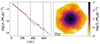 |
Fig. 1. Example of the virialized stellar distribution of a progenitor with M⋆ = 5.48 × 10³ M⊙ and R1/2 = 118 pc generated using DICE (see Sect. 2.1.3). Left panel: Stellar density (ρ⋆) extracted by spherically averaging the mass in a simulation shell (points) and the fit exponential profile (solid line, Eq. (4)) as a function of the radius (r). Right panel: Stellar surface density map, Σ⋆ integrated along the line of sight; the spatial scale is indicated as an inset. In both panels, the dashed lines mark the location of spheres with radius R1/2, 3 R1/2, and 5 R1/2. |
2.1.4. Merger setup
Using DICE, we placed the two progenitors in the simulation box, assigned them a relative velocity, set the system’s center of mass at rest in the center, and placed the progenitors at a distance of D = 8 kpc along the X axis, which ensured that they virialized while the gravitational interaction was still negligible. Hereafter, the subscript 1 refers to the more massive progenitor and 2 to the other one.
We set the progenitors on the same Z axis, assuming that the velocity differs from zero only along the X axis. The initial position of the progenitors can be written as
 (5a)
(5a)
 (5b)
(5b)
with their velocity along the X axis being
 (5c)
(5c)
In Eq. (5), Mi is the total mass of the i-th progenitor (Mi = Mi,DM + Mi,⋆), l is the specific angular momentum (with regard to the center of mass),
 (6a)
(6a)
where the sum over s is extended to all particles, and k is the specific kinetic energy,
 (6b)
(6b)
We varied the values of l and k to probe different merging trajectories. Figure 2 shows an example of the merger’s ICs, in which the two progenitors have total masses of M1 = 4.8 × 10⁷ M⊙ and M2 = 4.6 × 10⁶ M⊙, the specific merger kinetic energy is k = 0.72 pc2 Myr−2, and the angular momentum is l = 1.1 × 10³ pc2 Myr−1.
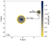 |
Fig. 2. Example of merger ICs prepared with DICE (see Sect. 2.1.4). The density map in the X − Y plane shows the total (dark matter+stars) density (ρ) that has been mass-averaged along the Z axis. The two progenitors were placed in the simulation box at a distance of D = 8 kpc along the X axis and with an impact parameter of |Y1|+|Y2| (Eq. (5b)). The arrows mark the direction of the initial velocity of each progenitor (Eq. (5c)). |
2.2. Parameterization of the merger
We focus our exploration on the five parameters: the merger mass ratio, M1/M2, the dark matter content, MDM/M⋆, the stellar radius of the progenitors, R1/2, the specific angular momentum, l, and the specific kinetic energy, k. In the following, we first describe the interval explored for each of these properties and then present how we explore the parameter space via a Latin hypercube sampling. Table 1 summarizes the properties and relative intervals explored.
2.2.1. Merger mass ratio
Defining the merger mass ratio between the two progenitors as M1/M2, we note that previous works (e.g., Deason et al. 2022) identify a peak in the fraction of stars in the stellar halo when M1/M2 ≃ 5. Therefore, to fully capture its dependency in UFD mergers, we explored the interval M1/M2 ∈ [1, 30].
It is convenient to use the merger mass ratio to define the stellar mass of each progenitor:
 (7a)
(7a)
 (7b)
(7b)
where Mtot, ⋆ = M1, ⋆ + M2, ⋆ is the total stellar mass in the simulation, which was set to Mtot, ⋆ = 6 × 10³ M⊙ to ensure that, even in the case of stellar mass loss during the merger, the post-merging galaxy stellar mass is consistent with Tucana II estimations,  (Bechtol et al. 2015).
2.2.2. Dark matter to stellar mass ratio
The dark matter content of UFDs is poorly constrained. Velocity dispersion observations can determine the dark matter mass within the luminous part of the galaxy; however, extrapolating the total halo masses from such a measurement is an uncertain endeavor (e.g., Errani et al. 2018). For this reason, we explored an interval of values of MDM, investigating whether the dark matter abundance impacts the stellar halo formation. To this end, we varied the stellar to dark matter mass ratio, MDM/M⋆, which determines the dark matter mass of each progenitor once the merger mass ratio sets the stellar mass.
The interval explored is MDM/M⋆ ∈ [8, 100]×103, and, in Fig. 3, we report it in an M⋆ - MDM plane with a shaded region. The selected range includes the latest dark matter mass estimate within 1 kpc for Tucana II,  (Chiti et al. 2021). Further, the explored range roughly brackets the predictions by abundance-matching methods performed by Behroozi et al. (2013) for galaxies between z = 6 and z = 0 (green lines in Fig. 3). Recently, a substantial effort has been carried out to constraint the stellar mass for smaller system both from local galaxy observations (e.g., Jethwa et al. 2018; Nadler et al. 2020) and simulations (e.g., Munshi et al. 2021; Kim et al. 2024). The explored range in this work encompasses most of the scatter measured at z = 0 in simulated dwarf galaxies by Kim et al. (2024, green-shaded area in Fig. 3).
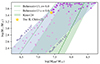 |
Fig. 3. Parameter sampling in the dark matter (MDM) vs. stellar mass (M⋆) plane. Each pink (purple) point represents the least (more) massive progenitor in a merging simulation. The shaded blue region indicates the dark matter to stellar mass (MDM/M⋆) interval explored by the suite. The gold star shows the estimate of Tucana II from Chiti et al. (2021) observations, while the green lines are the extrapolation from the abundance matching model from Behroozi et al. (2013) at redshift z = 0 and 6. The shaded green region represents the extrapolation of the scatter in the stellar-mass to halo-mass relation measured by Kim et al. (2024) for dwarf galaxies. |
2.2.3. Half-mass radius
Observations show that UFDs with a stellar mass similar to Tucana II have a half-light radius – the radius that contains half of the galaxy’s luminosity – ranging from tens to hundreds of parsecs (Simon 2019). The half-light radius is equal to the half-mass radius, assuming a constant luminosity-to-mass ratio, and thus we decided to explore an interval of values, R1/2 ∈ [15, 150] pc.
We assigned the value of R1/2 to the more massive progenitor, and we defined the mean stellar density as
 (8)
(8)
To set the scale radius of the other progenitor, we imposed that the two galaxies have the same  ; that is, the scale radius of the less massive was determined by R1/2(M2/M1)1/3. This approach prevented us from exploring the dependency of the stellar halo formation on the density difference between the two progenitors. However, by avoiding double sampling the R1/2 parameter, we reduced the number of dimensions explored, thereby improving the robustness of our results.
In Fig. 4, we report the sampling of the M⋆-R1/2. We considered the stellar mass and half-light radii of all the UFDs in the Local Universe Database (Pace 2024) and performed a fit with a polynomial function. The fit ±1 − σ range is reported as the green-shaded area in Fig. 4. The overlap between the sampled values and the observations in the M⋆-R1/2 plane confirms that the adopted scaling and range of the radii are adequate to explore the physical parameter space.
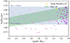 |
Fig. 4. Parameter sampling in the stellar mass (M⋆) vs. scale radius (R1/2) plane. Each pink (purple) point represents the least (more) massive progenitor in a merging simulation and the shaded blue area indicates the scale radius interval explored in the suite. The shaded green region represents the polynomial fit ±1σ of all the available UFD data in the Local Volume Database (Pace 2024). |
2.2.4. Specific angular momentum and kinetic energy
Since we want to study the merging event between galaxies, we limited our explorations to values of l and k that are highly likely to produce the merging of the two progenitors. Specifically, the intervals explored are l ∈ [100, 3000] pc2 Myr−1 and k ∈ [0.1, 3] pc2 Myr−2. We adopted these intervals after testing them with (i) the solution of the two-body problem, assuming both galaxies as point masses, and (ii) a low-resolution version of the simulation suite, as is further explained in the following.
2.3. Parameter space sampling
Sampling the parameter space is a delicate endeavor. The more samples we have, the more finely we explore the parameter space, with increasing computational cost. We used a five-dimensional Latin hypercube sampling (McKay et al. 1979) to maximize the exploration, while keeping the number of samples (simulations) low. The implemented sampling consists of 47 nodes (sampled points) with each node being a unique set of the five parameters defining the merger; that is,
 (9)
(9)
To compute the node values with the LHS prescription, we divided the range of each individual parameter into a set of equally probable intervals and the algorithm selected one sample from each interval, ensuring that the samples were evenly spaced out across the entire range. We adopted a logarithmic scaling for the five components in the node κ.
We verified that the progenitors were on merging trajectories before evolving the ICs generated by the 47 nodes at full resolution. To do so, we generated the ICs at lower dark matter resolution,  , and evolved them. The coarser resolution makes these simulations run at around a tenth of the computational cost, enabling us to evolve each one for 5 Gyr and check whether or not the progenitors merge. In addition, having the same ICs simulated using two different resolutions allows us to evaluate the resolution effects, as is detailed in Appendix A.
2.4. Time evolution
We used the public version of the moving-mesh hydrodynamic code AREPO (Springel 2010; Weinberger et al. 2020) to evolve the ICs. AREPO performs the time evolution with a second-order accurate leapfrog scheme, using a tree-particle-mesh method (Bagla 2002) to compute the gravitational interaction between particles. Having just two galaxies in the simulation box, we adopted only the oct-tree grouping scheme (Barnes & Hut 1986) for the force evaluation, using nonperiodic boundary conditions. The gravitational softening length of dark matter and stellar particles is ϵ = 1 pc, and the simulation box has side L = 100 kpc.
Each simulation evolved until the two progenitors merged into a single, virialized galaxy. The merging instant was identified using the on-the-fly friends-of-friends group finder (FoF) available within AREPO and originally described in Springel et al. (2001). The algorithm groups together particles within a distance of 0.2 times the mean interparticle separation. We defined the merging instant as the point at which the FoF algorithm finds a single galaxy. After the merging instant, each simulation evolves for an additional ∼1 Gyr, to ensure that the two progenitors fully merge and that the virial ratio is 2T/U ≃ 1 for several hundred million years, with T being the kinetic energy and U the potential energy.
2.5. Merger emulator
Having a high computational cost is a common limitation in numerical simulations, especially when a parameter space exploration is involved; a possible solution is the implementation of an emulator, to either reduce the number of simulations needed (e.g., Bird et al. 2019; Rogers et al. 2019; Brown et al. 2024) or to speed up the computation (e.g., Spurio Mancini et al. 2022; Branca & Pallottini 2024; Robinson et al. 2024; Bartlett et al. 2024). In this work, we have adopted a neural network (NN) as an emulator to enhance the parameter space exploration. The NN approximates a function that, taking the merger configuration and progenitor ICs as input, returns the properties of the post-merger galaxy without requiring new simulations. Indeed, thanks to the universal approximation theorem (UAT, Cybenko 1989), a trained NN can approximate with arbitrary precision the nonlinear function that maps the input parameters, κ, into outputs characterizing the galaxy and the stellar halo. For the present work, we set two outputs,
 (10)
(10)
where with R⋆ we refer to the half-mass radius of the post-merger galaxy to distinguish it from the massive progenitor’s half-mass radius, R1/2, which is one of the inputs of the NN. f5 is the stellar halo mass fraction; that is, the fraction of stars at r > 5R⋆. Such a choice of outputs enables us to directly compare our results with Tucana II observations (see Sects. 3.2 and 3.3).
We adopted a regularized loss function to prevent overfitting and trained the emulator on the simulation outputs. The number of training points is small compared to the dimensionality of the problem and we overcame the sparse sampling issue by adopting a Latin hypercube sampling (see Sect. 2.3), which ensures uniform coverage of the parameter space. Furthermore, deep NNs are relatively unaffected by the growing difficulty of analyzing data as the number of dimensions increases; that is, the “curse of dimensionality”, when approximating compositional functions (Poggio & Liao 2018). We refer to Appendix B for a complete description of the NN.
3. Results
First, we present the evolution of a single simulation and its analysis to overview the merging process (Sect. 3.1). Then, we repeat the same analysis on all the simulations, use the results to train the emulator, and explore the parameter space to determine the dependency of the stellar halo on the ICs (Sect. 3.2). Finally, we directly compare our findings with the observations of Tucana II (Sect. 3.3).
3.1. Merging of ultra-faint dwarfs: An overview
To showcase the merging process, we selected simulation SIM_47, which produces a post-merger galaxy with a stellar surface density consistent with the one observed in Tucana II (see Sect. 3.3). Simulation SIM_47 has a merger mass ratio of M1/M2 ≃ 10, scale radius of R1/2 ≃ 120 pc, mass-to-light ratio of MDM/M⋆ ≃ 104, specific angular momentum of l ≃ 1.1 × 10³ pc2 Myr−1, and specific kinetic energy of k ≃ 0.72 pc2 Myr−2. We note that this is the set of parameters already used in Figs. 1 and 2, which show the ICs and merger setup, respectively.
To visualize the spatial evolution in the simulated volume, we report the stellar surface density for the various phases of the merger in Fig. 5. The top left panel is at t = 0.2 Gyr when the two progenitors are virialized. The top right panel shows the gravitational interaction between the two progenitors during the third and last passage before merger completion. The bottom panels are at the end of the simulation; that is, at t = 4.01 Gyr, when the post-merger galaxy is virialized, and when the virial ratio is around 1. The effect of the merger on the morphology of the galaxy is evident when comparing the post-merger galaxy with one of its progenitors (the right panel in Fig. 1). To help the comparison, we mark 1, 3, and 5 R⋆ in both panels of Fig. 1 and Fig. 5. The progenitor is mostly contained within 5 R1/2, while the post-merger galaxy is wider, extending way beyond 5 R⋆. The extended stellar distribution at large radii – the stellar halo – forms as a result of the merger event and is bar-shaped. Therefore, contrary to the progenitors, the post-merger galaxy is asymmetric and we account for the asymmetry using an ensemble average2 to estimate R⋆, which we recall is the half-mass radius of the 2D projection of the galaxy. We address the differences between the 3D and 2D half-mass radius in Appendix C.
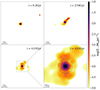 |
Fig. 5. Example of merger evolution. The different panels report the stellar surface density (Σ⋆) maps at various evolutionary stages for progenitors with a M1/M2 ≃ 10 (profile in Fig. 1) and the merger setup in Fig. 2. The bottom right panel is a zoom-in on the virialized post-merger galaxy, and the three dashed circles have radii of one, three, and five half-mass radii. After the merging, the resulting fraction of stars in the outskirts is f5 ∼ 5.5%. |
To analyze the difference between pre- and post-merger galaxies’ stellar distribution, in Fig. 6 we compare the stellar density of the two progenitors (shades of purple) and the post-merger galaxy (orange). The vertical lines are the half-mass radius for each galaxy, while the solid lines are the fit profiles: exponential (Eq. (4)) for both progenitors and the sum of two exponential profiles for the post-merger galaxy. The double exponential profile models the formation of a dense core and a sparse stellar halo and better fits the post-merger stellar distribution. The difference between the post-merger galaxy and its massive progenitor stellar distribution lies in the outskirts, where the post-merger galaxy has a higher mass fraction due to the formation of a stellar halo. The higher mass fraction affects the half-mass radius, going from R1/2 = (114 ± 1) pc of the massive progenitor to  pc of the post-merger galaxy. The error distribution in R⋆ is due to the asymmetry of the stellar halo formed via a merger.
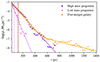 |
Fig. 6. Example of pre- vs. post-merging stellar distributions. We show the profile for the simulation selected for Fig. 5 by reporting ρ⋆ for the two progenitors with shades of purple and the post-merger galaxy in orange. The solid lines are the fit profile, which is exponential (Eq. (4)) and a sum of exponential for the progenitors and the post-merger galaxy, respectively. The vertical lines mark the half-mass radius for each galaxy. |
Tidal interactions during the merger strip stars from the less massive progenitor and form the stellar halo, as is shown in Fig. 7, where we report the fraction of stars of the post-merger galaxy coming from each progenitor at different radii. We adopted the same progenitor colors of Fig. 6, and the dashed lines are at 1, 3, and 5 R⋆. While the center of the post-merger galaxy is dominated by stars of the more massive progenitor, beyond 3 R⋆ the majority of the stars come from the smaller progenitor. This distribution shows that stars of the low-mass progenitor compose the stellar halo, and this is key to understanding the trends we observe exploring the parameter space (Sect. 3.2).
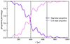 |
Fig. 7. Origin of the stars in the post-merger galaxy. For the simulation selected for Fig. 6, we show the radial distribution of the fraction of stars that originally belonged to the high-mass progenitor (purple) and the low-mass progenitor (pink). The dashed vertical lines are at 1, 3, and 5 R⋆. |
To quantify the presence of a stellar halo, we followed Tarumi et al. (2021) and calculated f5, which we recall is the fraction of stars beyond 5 R1/2. Since f5 depends on the half-mass radius, we performed the same ensemble average considering all possible projection planes. For each projection plane, we randomly sampled the stellar surface density distribution using the same number of stars of Chiti et al. (2021, i.e. 19) and considered the mean and standard deviation as f5 and its error. We refer the reader to Appendix C for a discussion on the differences between 3D and projected properties. We estimate f5 = 0.16 ± 0.4% and f5 = 0.19 ± 0.03% for the two progenitors. These values are consistent with the ones expected in isolated galaxies with an exponential profile, where f5 tends to zero. Figure 5 shows the formation of a stellar halo after the merger, and as a result of the stellar halo formation, the fraction of outskirts stars in the post-merger galaxy increases to f5 = 5.4 ± 1.8%. For comparison, the observed value in Tucana II is f5TucII = 2/19 = 10.5%.
3.2. Exploration of the parameter space with the emulator
Using the radius, R⋆, and the fraction of stars in the outskirts, f5, of each post-merger galaxy, we built the dataset to train the emulator. We recall that (Sect. 2.5) the input values of the emulator are the explored initial parameters, l, k, M1/M2, MDM/M⋆, and R1/2, and the output values are the median of the two post-merger quantities, f5 and R⋆ (see Eq. (10); for details of the NN architecture and its training, we refer to Appendix B).
Figure 8 shows the distribution of the emulated outputs (f5 top row, R⋆ bottom row) of 106 different ICs log-spaced distributed. The orange dots represent the results of the training simulations, and their overlap with the emulated results confirms the emulator’s robustness. The last column of Fig. 8 shows the distribution of output values in the parameter space explored. The distribution of f5 peaks around 5%, the value found by Tarumi et al. (2021) for their dry merger. The R⋆ distribution increases at low values. This trend is primarily due to the distribution of the training data, which is affected by numerical heating at low R1/2, as is explained in detail in Appendix A. Consequently, the emulator predicts a higher frequency of galaxies with low R⋆ due to the higher number of simulations with R⋆ ≃ 40 pc.
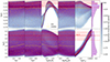 |
Fig. 8. Emulation of the post-merging f5 (upper panels) and stellar radius (R⋆, lower panels) as a function of merger setup parameters, i.e., specific angular momentum (l, Eq. (6a)), specific kinetic energy (k, Eq. (6b)), mass ratio (M1/M2), dark to stellar mass ratio (MDM/M⋆), and pre-merger stellar size (R1/2, Eq. (4)). Each of the first five columns gives the distribution of outputs of the merging process as a function of a single parameter. The distribution is obtained by emulating 106 IC log-spaced distributed (see Table 1), and the gold line represents its median. The orange points are the individual simulations used to train the emulator. The red line (shaded region) gives the average (dispersion) of the observed values for Tucana II (Bechtol et al. 2015; Chiti et al. 2021). The last column shows the distribution of the emulated output normalized to the total number of inferences. |
The red-shaded areas are the observed values for Tucana II with the relative error. There are several estimates of the angular size of Tucana II (Bechtol et al. 2015; Koposov et al. 2015; Moskowitz & Walker 2020) and distances (Bechtol et al. 2015; Koposov et al. 2015; Vivas et al. 2020) each resulting in different half-light radii. To ensure consistency with Chiti et al. (2021), we adopted the half-light radius  pc (Bechtol et al. 2015). This choice allows for a direct comparison of our simulated stellar distribution with their observational data. We computed the fraction of distant stars, f5TucII = 10 ± 5%, from the distribution of individual stars observed in Chiti et al. (2021). The error assigned to f5 considers that one of the two stars in the outskirts can lie within 5 R1/2, changing the fraction to 5%.
The emulated results, whose median is given by the gold line, show little to no dependency on the specific angular momentum, l, kinetic energy, k, and dark matter content, MDM/M⋆. Clear trends are instead present for the merger mass ratio, M1/M2, and the progenitor half-mass radius, R1/2; specifically, R⋆ correlates almost linearly with R1/2, while f5 increases with M1/M2, peaks around M1/M2 ≃ 6, and then decreases. The correlation between the sizes of the progenitor and the post-merger galaxy is expected, since the larger the progenitor is, the larger the post-merger galaxy will be. Meanwhile, the correlation between f5 and the merger mass ratio emerges because, as is discussed in Sect. 3.1, the stellar halo stars primarily originate from the less massive progenitor (the “satellite”), leading to two distinct regimes. When the two progenitors have comparable masses, they mix, forming a post-merger galaxy with a minimal stellar halo and a small f5. In this regime, increasing the merger mass ratio weakens the depth of the potential well of the satellite, making it easier for its stars to be stripped during the merger and form a more prominent stellar halo. As a result, f5 initially increases with the M1/M2 ratio. However, increasing M1/M2 reduces the number of stars in the “satellite”, leading to a decrease in the number of stars available to form the stellar halo. For this reason, beyond a certain threshold (approximately M1/M2 ≃ 6), f5 begins to decline.
To quantify the dependencies of f5 and R⋆ from the ICs (κ), we performed a principal component analysis (PCA). A PCA studies the linear transformation (component) of the parameter space of the data. Such components are ranked so that the variance decreases. Thus, the first (principal) components can explain most of the variation in the original dataset. We performed the PCA separately for the two outputs; that is, one for (f5, κ) and one for (R⋆, κ). For each PCA, we considered 106 points in six dimensions, normalizing each dimension such that its mean and standard deviation are 0 and 1, respectively. The first PCA component for f5 (R⋆) is dominated by f5 (R⋆) and M1/M2 (R1/2), confirming the trends observed in Fig. 8.
To determine the secondary dependencies, we performed two additional PCAs considering a reduced number of points. Specifically, when analyzing f5, we considered the points with M1/M2 ∈ [5, 7], where f5 peaks, while for R⋆, we considered the points with the progenitor radius R1/2 ∈ [90, 110] pc; that is, the progenitor radius producing a post-merger galaxy radius consistent with Tucana II observations. The first reduced PCA component for f5 (R⋆) is dominated by f5 (R⋆) and R1/2 (M1/M2), revealing that the principal dependency of one output is the secondary dependency of the other.
Once we removed the dependency on M1/M2 and R1/2, selecting points simultaneously in the intervals M1/M2 ∈ [5, 7] and R1/2 ∈ [125, 145] pc, we noticed that f5 and R⋆ marginally depend on the other three parameters, l, k, and MDM/M⋆. The relative importance depends on the intervals considered, but generally MDM/M⋆ is the least important for both f5 and R⋆.
3.3. Comparison with Tucana II observations
We can now compare the emulated f5 and R⋆ with the observations to infer the properties of Tucana II progenitors. As is described in Sect. 3.2, we adopted  pc and f5TucII = 10 ± 5% as observed values of half-mass radius and fraction of stellar halo stars in Tucana II, respectively.
Figure 9 shows the distribution of the output values consistent with Tucana II observations, and based on the PCA results, we limited the study to two initial parameters that define the output values; that is, M1/M2 and R1/2. The top row shows the distribution of these initial parameters, with the dashed lines indicating the median and 16-th and 84-th percentiles, while the four orange points represent four simulations in the suite consistent with Tucana II observations. Consistency with observations is achieved for ICs with a progenitor half-mass radius of  pc and a merger mass ratio of
  . Therefore, we determine that an intermediate merger (5 < M1/M2 < 12) forms a stellar halo similar to the one observed for Tucana II. Such a finding is consistent with Deason et al. (2014), who report that 40% of z = 0 UFDs in their simulations underwent at least one major merger in the last 12 Gyr. Among the four post-merger simulations consistent with observations, SIM_41 and SIM_47 are consistent within 1.1σ with3 the inferred values of M1/M2 and R1/2, SIM_17 has a slightly larger progenitor radius, > 1.1σ, and SIM_39 has both M1/M2 and R1/2 values > 1.1σ. We note that the errors on the inferred properties highly depend on the value and error adopted for f5, and better constraining it helps to decrease the uncertainties on M1/M2 and R1/2. For example, lowering f5 error by a factor of two – ∼ ± 2.5% – results in a decrease of a factor of three on the error of the ICs consistent with Tucana II.
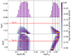 |
Fig. 9. Distributions of the input couple R1/2 and M1/M2 that give f5 and R⋆ simultaneously consistent with the observations from Tucana II. Similarly to Fig. 8, the red line gives the average value inferred from observations, but the ranges for f5 and R⋆ were cut to include only the observational uncertainty, i.e., f5TucII = 10 ± 5% (Chiti et al. 2021) and |
One method to reduce the error on f5 is to increase the number of identified stars; for example, using Gaia data. In recent work, Jensen et al. (2024) exploit Gaia data, employing a selection algorithm based on spatial, color-magnitude, and proper motion information targeting low brightness features of MW dwarf satellites. They are able to identify the second low-density outer profile of nine satellites, including Tucana II, and for each of them, to derive the stellar surface density profile. They model it as the sum of two exponential profiles:
 (11)
(11)
where Σ0 is the central surface density, re is the exponential scale radius, B is the normalization of the outer component (0 ≤ B ≤ 1), and rs the scale radius of the outer component (1.68rs > R1/2). They derive re from the literature value of the half-light radius such that R1/2 = 1.68re. Unfortunately, we cannot use their star candidates list to evaluate f5, since there are no spectroscopic follow-ups to verify the membership of each star. However, we can test our results by comparing the surface density of our simulated post-merger galaxies with the one derived by them.
Figure 10 shows the derived stellar surface density profile of Tucana II (green) and our simulated post-merger galaxies (orange), and each of the four columns refers to a simulation that is simultaneously consistent with the observed values of f5 and R1/2. As we can see, most of these four simulations reasonably match the observed stellar halo well beyond 1 kpc and only SIM_39 is not consistent with the observed data. We quantified the accordance between simulations and observations using the standard χ2 procedure:
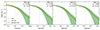 |
Fig. 10. Comparison of the observed stellar number density distribution of Tucana II and the simulations with the f5 and R1/2 parameters closest to the observed values (f5TucII = 10 ± 5% from Chiti et al. 2021 and |
 (12)
(12)
where Σi, obs (σi, obs) and Σi, sim (σi, sim) are the stellar surface density profiles (standard errors) derived from observations and simulations, respectively. We used ten radius bins to be consistent with Jensen et al. (2024), and for each bin we computed σi, obs propagating R1/2, B, and rs errors, and we computed σi, sim as the Poisson error. The three simulations within 1.1σ from the inferred M1/M2 – SIM_17, SIM_41, and SIM_47 – have a good agreement; that is, χ2 = 0.5 − 2. It should be noted that χ2 of SIM_17 is larger, since the accordance with R1/2 is worse. All three simulations show the two-component profiles with differences in the central density Σ0 and the transition to the second exponential profile. Their ICs span almost all the angular momentum values, confirming that the formation of a stellar halo does not depend on angular momentum in the interval explored in this work. We recall that we considered l values that result in a merger between the two progenitors. For SIM_39, the surface density significantly diverges from the observed one (χ2 = 12.0). Although the fraction of distant stars is consistent with observations,  , the simulation features an inner core that is 2× denser and 0.5× smaller compared to observations. This is due to the offset from M1/M2 and R1/2, which are at > 1.1 σ from the emulator predictions.
4. Summary and discussion
In this work, we investigate merger events as the formation scenario of stellar halos around UFDs. We study the impact of different merger and progenitor properties and focus on reproducing the stellar halo observed in Tucana II by Chiti et al. (2021, 2023), Jensen et al. (2024).
To this end, we developed a suite of 47 N-body simulations of isolated dry mergers between two idealized progenitors of Tucana II with a stellar resolution of a single solar mass. We used DICE (Perret 2016) to generate the ICs, assuming an exponential profile for the stellar component of both progenitors, and we used AREPO (Weinberger et al. 2020) to evolve the simulation until the post-merger galaxy virializes. The suite explores different merger trajectories and progenitors properties, assigning to each simulation a unique set of five parameters: i) the specific angular momentum, l, ii) the specific kinetic energy, k, iii) the merger mass ratio, M1/M2, iv) the dark matter content, MDM/M⋆, and v) the half-mass radius of the more massive progenitor, R1/2. For each post-merger galaxy, we quantified the formation of a stellar halo using two properties: the half-mass radius, R⋆, and the fraction of stars, f5, at high radii (> 5R⋆).
We developed a NN-based emulator to avoid the extreme computational cost expected from a high-resolution sampling of the selected five-dimensional parameter space. Via the emulator, we quickly obtained the properties of one million post-merger galaxies – R⋆ and f5 – and studied the dependency of the stellar halo formation on the ICs of the merger and progenitors. By comparing the emulated properties to Tucana II observations, we inferred consistent merger and progenitor characteristics. Additionally, we compared the stellar surface density of simulated post-merger galaxies and Tucana II to further validate the merger scenario.
We can summarize our most important results as follows:
-
The merger mass ratio, M1/M2 (progenitors’ size, R1/2), drives the formation of a stellar halo, f5 (the size of the galaxy, R⋆), in the aftermath of a merger, with the progenitors’ size, R1/2 (merger mass ratio, M1/M2), being the secondary dependency. In the interval explored, the specific angular momentum, l, specific kinetic energy, k, and dark matter abundance, MDM/M⋆, have a negligible impact on both the stellar halo formation and the size of the post-merger galaxy.
-
Using the observed fraction of distant stars, f5TucII = 10.5% (Chiti et al. 2021), and half-light radius, R⋆TucII = 120 pc (Bechtol et al. 2015), of Tucana II, we predict that the merger mass ratio and massive progenitor size consistent with observations are
 and
and  pc. The merger that can form Tucana II’s stellar halo is intermediate, while the size of present-day Tucana II is similar to the radius of its massive progenitor.
 -
Four simulated post-merger galaxies are consistent with f5TucII and R⋆TucII. Three simulations have M1/M2 (R1/2) within 1.1σ (1.2σ) from the predicted values: their stellar surface density reproduce (χ2 ≈ 0.5 − 2) the observed one (Jensen et al. 2024) well. The simulation with both M1/M2 and R1/2 at > 1.2σ from the predictions deviates the most from observations (χ2 = 12). This underlines the importance of M1/M2 and R1/2 in determining the post-merger galaxy morphology.
Our results confirm previous findings about the importance of the merger mass ratio on the formation of a stellar halo in UFDs (Deason et al. 2022; Ricotti et al. 2022), show the impact of the progenitor size on the radius of the post-merger galaxy, and highlight the possibility of inferring progenitor and merger properties using present-day observations. The agreement between the results from our simulations and emulations with observations in terms of f5, R⋆, and stellar surface density further corroborates the merging scenario for the formation of Tucana II’s stellar halo, suggested by observations (Chiti et al. 2021, 2023) and simulations of two specific UFD progenitors (Tarumi et al. 2021).
The NN-based emulator proves to be a fundamental tool to perform the parameter space exploration, especially when computational resources are limited, and it can be easily adapted to infer any scalar property from simulations; for example, the post-merger galaxy’s total mass. To emulate functional properties, such as the parametrical dependence of density profiles or surface brightness, and directly compare them with observations (e.g. Jensen et al. 2024; Conroy et al. 2024), it is required to change the architecture to a neural operator-based model (Lu et al. 2019). Such a possibility highlights the versatility and power of emulation techniques in astrophysical research.
We expect ongoing and future spectroscopic surveys targeting UFDs to have a high impact on the search for stellar halos. For example, 4DWARFS (Skúladóttir et al. 2023) will provide the chemical abundances for more than 2000 stars in ∼40 UFDs (Skúladóttir, private communication). The higher statistic will produce precise measurements of f5 in Tucana II and possibly other UDFs, revealing the frequency of stellar halos around UFDs. Using our method on this upcoming data will allow us to uncover the past assembly history of the faintest companions of our MW.
The cosmological parameters adopted in this work are taken from Planck Collaboration XIII (2016): H0 = 67.74 km s−1 Mpc−1, Ωm = 0.3089, and ΩΛ = 0.6911.
We consider all possible projection planes, take the median as R1/2 and the 16-th and 84-th percentiles as the error.
For the results of our models, the left (right) σ is defined as the interval between the 16-th (84-th) percentile and the median. Different definitions of σ give slight quantitative differences, but the physical picture is unchanged.
Acknowledgments
This project received funding from the ERC Starting Grant NEFERTITI H2020/804240 (PI: Salvadori). We acknowledge the CINECA award under the ISCRA initiative for the availability of high-performance computing resources and support from the Class C project UFD-SHF, “UFD mergers: Stellar Halo Formation”, HP10CM106H (PI: Querci). We acknowledge the usage of AREPO (Weinberger et al. 2020), ASTROPY (The Astropy Collaboration 2022), DEEPXDE (Lu et al. 2021), DICE (Perret 2016), MATPLOTLIB (Hunter 2007), NUMPY (Harris et al. 2020), PYNBODY (Pontzen et al. 2013), PYTHON3 (Van Rossum & Drake 2009), SCIPY (Virtanen et al. 2020), and SCIKIT LEARN (Pedregosa et al. 2011).
References
- Agertz, O., Pontzen, A., Read, J. I., et al. 2020, MNRAS, 491, 1656 [Google Scholar]
- Bagla, J. S. 2002, JApA, 23, 185 [NASA ADS] [Google Scholar]
- Barkana, R., & Loeb, A. 1999, ApJ, 523, 54 [NASA ADS] [CrossRef] [Google Scholar]
- Barnes, J., & Hut, P. 1986, Nature, 324, 446 [NASA ADS] [CrossRef] [Google Scholar]
- Bartlett, D. J., Chiarenza, M., Doeser, L., & Leclercq, F. 2024, arXiv e-prints [arXiv:2409.02154] [Google Scholar]
- Battaglia, G., & Nipoti, C. 2022, Nat. Astron., 6, 659 [NASA ADS] [CrossRef] [Google Scholar]
- Bechtol, K., Drlica-Wagner, A., Balbinot, E., et al. 2015, ApJ, 807, 50 [NASA ADS] [CrossRef] [Google Scholar]
- Behroozi, P. S., Wechsler, R. H., & Conroy, C. 2013, ApJ, 770, 57 [NASA ADS] [CrossRef] [Google Scholar]
- Belokurov, V., Zucker, D. B., Evans, N. W., et al. 2006, ApJ, 647, L111 [NASA ADS] [CrossRef] [Google Scholar]
- Bird, S., Rogers, K. K., Peiris, H. V., et al. 2019, JCAP, 2019, 050 [CrossRef] [Google Scholar]
- Branca, L., & Pallottini, A. 2024, A&A, 684, A203 [NASA ADS] [CrossRef] [EDP Sciences] [Google Scholar]
- Brown, T. M., Tumlinson, J., Geha, M., et al. 2012, ApJ, 753, L21 [NASA ADS] [CrossRef] [Google Scholar]
- Brown, S. T., Fattahi, A., McCarthy, I. G., et al. 2024, MNRAS, 532, 1223 [NASA ADS] [CrossRef] [Google Scholar]
- Bühlmann, P., & van de Geer, S. 2011, Statistics for High-Dimensional Data: Methods, Theory and Applications, Springer Series in Statistics (Berlin, Heidelberg: Springer) [Google Scholar]
- Bullock, J. S., & Boylan-Kolchin, M. 2017, ARA&A, 55, 343 [Google Scholar]
- Chiti, A., Frebel, A., Ji, A. P., et al. 2018, ApJ, 857, 74 [NASA ADS] [CrossRef] [Google Scholar]
- Chiti, A., Frebel, A., Simon, J. D., et al. 2021, Nat. Astron., 5, 392 [NASA ADS] [CrossRef] [Google Scholar]
- Chiti, A., Frebel, A., Ji, A. P., et al. 2023, AJ, 165, 55 [NASA ADS] [CrossRef] [Google Scholar]
- Conroy, C., Johnson, B. D., van Dokkum, P., et al. 2024, ApJ, 968, 129 [NASA ADS] [CrossRef] [Google Scholar]
- Cybenko, G. 1989, Math. Control Signals Syst. (MCSS), 2, 303 [NASA ADS] [CrossRef] [Google Scholar]
- Deason, A., Wetzel, A., & Garrison-Kimmel, S. 2014, ApJ, 794, 115 [Google Scholar]
- Deason, A. J., Bose, S., Fattahi, A., et al. 2022, MNRAS, 511, 4044 [NASA ADS] [CrossRef] [Google Scholar]
- Di Cintio, P. 2024, A&A, 683, A254 [NASA ADS] [CrossRef] [EDP Sciences] [Google Scholar]
- Diemer, B., & Kravtsov, A. V. 2015, ApJ, 799, 108 [Google Scholar]
- Errani, R., Peñarrubia, J., & Walker, M. G. 2018, MNRAS, 481, 5073 [CrossRef] [Google Scholar]
- Fattahi, A., Navarro, J. F., Frenk, C. S., et al. 2018, MNRAS, 476, 3816 [Google Scholar]
- Gallart, C., Monelli, M., Ruiz-Lara, T., et al. 2021, ApJ, 909, 192 [NASA ADS] [CrossRef] [Google Scholar]
- Garling, C., Willman, B., Sand, D. J., et al. 2018, ApJ, 852, 44 [NASA ADS] [CrossRef] [Google Scholar]
- Gelli, V., Salvadori, S., Pallottini, A., & Ferrara, A. 2020, MNRAS, 498, 4134 [NASA ADS] [CrossRef] [Google Scholar]
- Gelli, V., Salvadori, S., Ferrara, A., Pallottini, A., & Carniani, S. 2023, ApJ, 954, L11 [NASA ADS] [CrossRef] [Google Scholar]
- Goater, A., Read, J. I., Noël, N. E. D., et al. 2024, MNRAS, 527, 2403 [Google Scholar]
- Gutcke, T. A., Pfrommer, C., Bryan, G. L., et al. 2022, ApJ, 941, 120 [NASA ADS] [CrossRef] [Google Scholar]
- Hansen, T. T., Simon, J. D., Li, T. S., et al. 2024, ApJ, 968, 21 [NASA ADS] [CrossRef] [Google Scholar]
- Harris, C. R., Millman, K. J., van der Walt, S. J., et al. 2020, Nature, 585, 357 [NASA ADS] [CrossRef] [Google Scholar]
- Hunter, J. D. 2007, Comput. Sci. Eng., 9, 90 [NASA ADS] [CrossRef] [Google Scholar]
- Jensen, J., Hayes, C. R., Sestito, F., et al. 2024, MNRAS, 527, 4209 [Google Scholar]
- Jeon, M., Bromm, V., Pawlik, A. H., & Milosavljević, M. 2015, MNRAS, 452, 1152 [NASA ADS] [CrossRef] [Google Scholar]
- Jeon, M., Besla, G., & Bromm, V. 2017, ApJ, 848, 85 [NASA ADS] [CrossRef] [Google Scholar]
- Jethwa, P., Erkal, D., & Belokurov, V. 2018, MNRAS, 473, 2060 [NASA ADS] [CrossRef] [Google Scholar]
- Ji, A. P., Frebel, A., Ezzeddine, R., & Casey, A. R. 2016, ApJ, 832, L3 [CrossRef] [Google Scholar]
- Kim, S. Y., Read, J. I., Rey, M. P., et al. 2024, arXiv e-prints [arXiv:2408.15214] [Google Scholar]
- Kirby, E. N., Simon, J. D., Geha, M., Guhathakurta, P., & Frebel, A. 2008, ApJ, 685, L43 [NASA ADS] [CrossRef] [Google Scholar]
- Koposov, S. E., Belokurov, V., Torrealba, G., & Evans, N. W. 2015, ApJ, 805, 130 [NASA ADS] [CrossRef] [Google Scholar]
- Lai, D. K., Lee, Y. S., Bolte, M., et al. 2011, ApJ, 738, 51 [CrossRef] [Google Scholar]
- Li, T. S., Simon, J. D., Kuehn, K., et al. 2018, ApJ, 866, 22 [NASA ADS] [CrossRef] [Google Scholar]
- Longeard, N., Jablonka, P., Battaglia, G., et al. 2023, MNRAS, 525, 3086 [NASA ADS] [CrossRef] [Google Scholar]
- Lu, L., Jin, P., & Karniadakis, G. E. 2019, arXiv e-prints [arXiv:1910.03193] [Google Scholar]
- Lu, L., Meng, X., Mao, Z., & Karniadakis, G. E. 2021, SIAM Rev., 63, 208 [CrossRef] [Google Scholar]
- Ludlow, A. D., Fall, S. M., Wilkinson, M. J., Schaye, J., & Obreschkow, D. 2023, MNRAS, 525, 5614 [NASA ADS] [CrossRef] [Google Scholar]
- Magg, M., Hartwig, T., Agarwal, B., et al. 2018, MNRAS, 473, 5308 [CrossRef] [Google Scholar]
- Martin, N. F., de Jong, J. T. A., & Rix, H.-W. 2008, ApJ, 684, 1075 [NASA ADS] [CrossRef] [Google Scholar]
- McConnachie, A. W. 2012, AJ, 144, 4 [Google Scholar]
- McKay, M. D., Beckman, R. J., & Conover, W. J. 1979, Technometrics, 21, 239 [Google Scholar]
- Moskowitz, A. G., & Walker, M. G. 2020, ApJ, 892, 27 [NASA ADS] [CrossRef] [Google Scholar]
- Muñoz, R. R., Côté, P., Santana, F. A., et al. 2018, ApJ, 860, 66 [CrossRef] [Google Scholar]
- Munshi, F., Brooks, A. M., Applebaum, E., et al. 2021, ApJ, 923, 35 [NASA ADS] [CrossRef] [Google Scholar]
- Nadler, E. O., Wechsler, R. H., Bechtol, K., et al. 2020, ApJ, 893, 48 [NASA ADS] [CrossRef] [Google Scholar]
- Navarro, J. F., Frenk, C. S., & White, S. D. M. 1996, ApJ, 462, 563 [Google Scholar]
- Oogi, T., Habe, A., & Ishiyama, T. 2015, MNRAS, 456, 300 [Google Scholar]
- Ou, X., Chiti, A., Shipp, N., et al. 2024, ApJ, 966, 33 [NASA ADS] [CrossRef] [Google Scholar]
- Pace, A. B. 2024, arXiv e-prints [arXiv:2411.07424] [Google Scholar]
- Pace, A. B., Erkal, D., & Li, T. S. 2022, ApJ, 940, 136 [NASA ADS] [CrossRef] [Google Scholar]
- Pallottini, A., & Ferrara, A. 2023, A&A, 677, L4 [NASA ADS] [CrossRef] [EDP Sciences] [Google Scholar]
- Pedregosa, F., Varoquaux, G., Gramfort, A., et al. 2011, J. Mach. Learn. Res., 12, 2825 [Google Scholar]
- Peñarrubia, J., Navarro, J. F., & McConnachie, A. W. 2008, ApJ, 673, 226 [Google Scholar]
- Perret, V. 2016, {ASCL}.net - {DICE}: {Disk} {Initial} {Conditions} {Environment}, Astrophysics Source Code Library [record ascl:1607.002] [Google Scholar]
- Planck Collaboration XIII. 2016, A&A, 594, A13 [NASA ADS] [CrossRef] [EDP Sciences] [Google Scholar]
- Poggio, T., & Liao, Q. 2018, Bull. Pol. Acad. Sci.: Tech. Sci., 66, 761 [Google Scholar]
- Pontzen, A., Roškar, R., Stinson, G., & Woods, R. 2013, pynbody: N-Body/SPH analysis for python, Astrophysics Source Code Library [record ascl:1305.002] [Google Scholar]
- Revaz, Y. 2023, A&A, 679, A2 [NASA ADS] [CrossRef] [EDP Sciences] [Google Scholar]
- Ricotti, M., & Gnedin, N. Y. 2005, ApJ, 629, 259 [NASA ADS] [CrossRef] [Google Scholar]
- Ricotti, M., Polisensky, E., & Cleland, E. 2022, MNRAS, 515, 302 [CrossRef] [Google Scholar]
- Robinson, D., Avestruz, C., & Gnedin, N. Y. 2024, arXiv e-prints [arXiv:2406.19446] [Google Scholar]
- Rogers, K. K., Peiris, H. V., Pontzen, A., et al. 2019, JCAP, 2019, 031 [CrossRef] [Google Scholar]
- Rossi, M., Salvadori, S., Skúladóttir, Á.., & Vanni, I. 2023, MNRAS, 522, L1 [NASA ADS] [CrossRef] [Google Scholar]
- Rossi, M., Salvadori, S., Skúladóttir, Á. Vanni, I., & Koutsouridou, I. 2024, ApJ, submitted [arXiv:2406.12960] [Google Scholar]
- Salvadori, S., & Ferrara, A. 2009, MNRAS, 395, L6 [NASA ADS] [Google Scholar]
- Salvadori, S., Tolstoy, E., Ferrara, A., & Zaroubi, S. 2014, MNRAS, 437, L26 [NASA ADS] [CrossRef] [Google Scholar]
- Salvadori, S., Skúladóttir, Á., & Tolstoy, E. 2015, MNRAS, 454, 1320 [Google Scholar]
- Shipp, N., Panithanpaisal, N., Necib, L., et al. 2023, ApJ, 949, 44 [NASA ADS] [CrossRef] [Google Scholar]
- Shipp, N., Riley, A. H., Simpson, C. M., et al. 2024, MNRAS, submitted [arXiv:2410.09143] [Google Scholar]
- Simon, J. D. 2019, ARA&A, 57, 375 [NASA ADS] [CrossRef] [Google Scholar]
- Skúladóttir, Á., Puls, A. A., Amarsi, A. M., et al. 2023, The Messenger, 190, 19 [Google Scholar]
- Sobacchi, E., & Mesinger, A. 2013, MNRAS, 432, 3340 [CrossRef] [Google Scholar]
- Spite, M., Spite, F., François, P., et al. 2018, A&A, 617, A56 [NASA ADS] [CrossRef] [EDP Sciences] [Google Scholar]
- Springel, V. 2010, MNRAS, 401, 791 [Google Scholar]
- Springel, V., Yoshida, N., & White, S. D. M. 2001, New Astron., 6, 79 [Google Scholar]
- Spurio Mancini, A., Piras, D., Alsing, J., Joachimi, B., & Hobson, M. P. 2022, MNRAS, 511, 1771 [NASA ADS] [CrossRef] [Google Scholar]
- Strigari, L. E. 2018, Rep. Prog. Phys., 81, 056901 [NASA ADS] [CrossRef] [Google Scholar]
- Sun, G., Faucher-Giguère, C.-A., Hayward, C. C., & Shen, X. 2023, MNRAS, 526, 2665 [NASA ADS] [CrossRef] [Google Scholar]
- Tarumi, Y., Yoshida, N., & Frebel, A. 2021, ApJ, 914, L10 [NASA ADS] [CrossRef] [Google Scholar]
- Tau, E. A., Vivas, A. K., & Martínez-Vázquez, C. E. 2024, AJ, 167, 57 [NASA ADS] [CrossRef] [Google Scholar]
- The Astropy Collaboration (Price-Whelan, A. M., et al.) 2022, ApJ, 935, 167 [NASA ADS] [CrossRef] [Google Scholar]
- Van Rossum, G., & Drake, F. L. 2009, Python 3 Reference Manual (Scotts Valley, CA: CreateSpace) [Google Scholar]
- Virtanen, P., Gommers, R., Oliphant, T. E., et al. 2020, Nat. Methods, 17, 261 [Google Scholar]
- Vivas, A. K., Martínez-Vázquez, C., & Walker, A. R. 2020, ApJS, 247, 35 [NASA ADS] [CrossRef] [Google Scholar]
- Waller, F., Venn, K. A., Sestito, F., et al. 2023, MNRAS, 519, 1349 [Google Scholar]
- Weinberger, R., Springel, V., & Pakmor, R. 2020, ApJS, 248, 32 [Google Scholar]
- Westmeier, T., Staveley-Smith, L., Calabretta, M., et al. 2015, MNRAS, 453, 338 [NASA ADS] [CrossRef] [Google Scholar]
- Wheeler, C., Hopkins, P. F., Pace, A. B., et al. 2019, MNRAS, 490, 4447 [CrossRef] [Google Scholar]
- Wolf, J., Martinez, G. D., Bullock, J. S., et al. 2010, MNRAS, 406, 1220 [NASA ADS] [Google Scholar]
- Yoon, J., Beers, T. C., Tian, D., & Whitten, D. D. 2019, ApJ, 878, 97 [Google Scholar]
Appendix A: Dynamical heating from dark matter resolution
Two species simulations, i.e. dark matter and stars, are affected by numerical heating that depends on the resolution mass ratio μ = mDM/m⋆ and on the number of particles (Ludlow et al. 2023). High μ or low number of particles induce numerical heating, resulting in spurious heating of the stellar component and a larger galaxy. To test the impact of numerical heating on our results, we compare the properties of the post-merger galaxies of three suites, varying the dark matter and stellar resolution. The dark matter particle of the low-resolution (high-resolution) suite has a mass of  (
( ) and the resolution mass ratio is μlow = 103 M⊙ (μhigh = 102). The mass of a single dark matter particle in the mid-resolution suite is
  while μmid = μhigh. The adopted μlow is similar to the value used by Agertz et al. (2020), while μhigh is consistent with the value in Ricotti et al. (2022).
In Fig. A.1, we show the distribution of the post-merger galaxies properties, f5 top row and R⋆ bottom row, in the parameter space explored. The high-resolution simulations are in orange, the mid-resolution in blue, and the low-resolution in green. Comparing the distributions of the fraction of distant stars, we note that they overlap, with the higher resolution suite peaking at a higher value (∼13%) compared to the mid-resolution (∼8.6%) and the low-resolution (∼8.2%). On the contrary, the half-mass distributions do not overlap, with the mid-resolution R⋆ systematically between the low- and high-resolution one.
Considering the typical error estimating f5, i.e., of the order of 20%, the f5 distributions at different resolutions are consistent. Such consistency confirms that the simulations capture the stellar halo formation by a dry merger, even with a resolution as low as  . On the contrary, the half-mass radius distributions do not overlap, even considering the error associated with the measure, showing the impact of spurious numerical heating and forcing a different method to test the convergence of the simulations. The size of the post-merger galaxy (orange points) is larger than the progenitor radius (the dashed line), as expected in N-body dry-merger simulations (Oogi et al. 2015) and evident from the bottom right panel of Fig. A.1. For R1/2 > 50 pc, the two radii are proportional, while below 50 pc R⋆ saturates at a minimum value, i.e., the radius resolution limit, suggesting that the numerical heating can be neglected in simulations with R1/2 > 50 pc. To further verify that numerical heating is negligible, we limit R1/2 to the proportional regime and determine the impact of each parameter on R⋆. We find the same hierarchy as when using the whole dataset, with R1/2 being the dominant parameter and M1/M2 playing a secondary role, showing that numerical heating does not affect our results. Moreover, the values of R⋆ derived at R1/2 ≃ 100 pc, i.e., the expected value of the massive progenitor radius consistent with observations, for different resolutions are consistent when considering the observational errors are of the order of ∼30 pc.
For the reasons stated above, our results on the stellar halo formation and size of the post-merger galaxies are well captured by the dark matter resolution  , and there is no need for increasing the resolution.
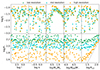 |
Fig. A.1. Comparison of the distribution of the post-merger galaxies properties, i.e., half-mass radius R⋆ (bottom row) and the fraction of stars f5 beyond 5R⋆ (top row), changing the dark matter and stellar resolution. Each column represents an IC property explored in this work, from left to right are: specific angular momentum l, specific kinetic energy k, merger mass ratio M1/M2, dark matter abundance MDM/M⋆, and progenitor half-mass radius R1/2. The dashed line in the bottom right corner is R⋆ = R1/2. The low-resolution simulations (mDM = 103 M⊙, mDM/m⋆ = 103 M⊙) are in green, the mid-resolution simulations are in blue (mDM = 103 M⊙, mDM/m⋆ = 102 M⊙), while the high-resolution simulations ( |

Appendix B: Using neural networks as an emulator
In this work, we adopt and train a NN as an emulator to infer an approximate value of f5 and R⋆ of post-merger galaxies based on the ICs of the merger. The NN has an input layer with 5 neurons, one for each parameter explored, i.e., l, k, M1/M2, MDM/M⋆, and R1/2, 5 hidden layers with 128 dense neurons, and an output layer with a neuron for f5 and R⋆, each.
The number of simulations available for training and testing the NN is limited, and each simulation carries information in a specific interval of ICs. To avoid losing information, we train the NN on all the available data, and we use a l2 regularization to control overfitting (Bühlmann & van de Geer 2011). We tested our approach by training nine identical emulators on 90%, 80%, and 70% of the dataset and testing them on the remaining fraction.
Figure B.1 shows the median of the inferred values of all emulators, colored by the training data size. All medians do not deviate more than 0.1 dex between each other, 0.05 dex in some cases, confirming that using all the available data to train the NN does not affect the results. Moreover, the primary and secondary dependencies on the properties of the IC and the inferred value of M1/M2 and R1/2 are consistent between all emulators, corroborating that our results do not critically depend on the training set of the NN.
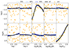 |
Fig. B.1. Same as Fig. A.1 considering only the high resolution simulation data in orange. Each line represents the median distribution of the reference emulator, black, or the test emulator, colored in shades of blue based on the size of the training set. |
Appendix C: Projecting 3D properties
Since the merger orbital plane is fixed in the suite, projecting both R1/2 and f5 on the XY plane can have systematic effects on the measures. To minimize such effects and to account for the asymmetry of the post-merger galaxies, we project the galaxy into 8000 different planes uniformly distributed in the 3D space and measure R1/2 and f5 for each projection. We take the median and 16%-th and 84%-th percentiles of the resulting distributions as the value and errors, respectively. The results of the ensemble average are shown in Fig. C.1, where each solid line represents a simulation and spans the interval between the 16%-th and the 84%-th percentile, and the dashed line is the plane’s bisector. As reported by Wolf et al. (2010), the ratio between the 2D and 3D half-mass radii can be approximated to 3/4 for many profiles, which is also true in our post-merger simulations. The 3D values of f5 are within the error bars of the projected f5, suggesting that the parameter is negligibly affected by the projection procedure.
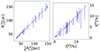 |
Fig. C.1. Distribution of the half-mass radius (left) and f5 (right) of the post-merger galaxy on the 3D-2D plane. Each solid line represents a simulation in the suite, spanning from the 16%-th to the 84%-th percentiles. The dashed lines in the two panels are the plane bisectors. The 3D half-mass value is multiplied by 3/4 to account for the projection, as reported by Wolf et al. (2010). |
All Tables
All Figures
|
Fig. 1. Example of the virialized stellar distribution of a progenitor with M⋆ = 5.48 × 10³ M⊙ and R1/2 = 118 pc generated using DICE (see Sect. 2.1.3). Left panel: Stellar density (ρ⋆) extracted by spherically averaging the mass in a simulation shell (points) and the fit exponential profile (solid line, Eq. (4)) as a function of the radius (r). Right panel: Stellar surface density map, Σ⋆ integrated along the line of sight; the spatial scale is indicated as an inset. In both panels, the dashed lines mark the location of spheres with radius R1/2, 3 R1/2, and 5 R1/2. |
| In the text | |
|
Fig. 2. Example of merger ICs prepared with DICE (see Sect. 2.1.4). The density map in the X − Y plane shows the total (dark matter+stars) density (ρ) that has been mass-averaged along the Z axis. The two progenitors were placed in the simulation box at a distance of D = 8 kpc along the X axis and with an impact parameter of |Y1|+|Y2| (Eq. (5b)). The arrows mark the direction of the initial velocity of each progenitor (Eq. (5c)). |
| In the text | |
|
Fig. 3. Parameter sampling in the dark matter (MDM) vs. stellar mass (M⋆) plane. Each pink (purple) point represents the least (more) massive progenitor in a merging simulation. The shaded blue region indicates the dark matter to stellar mass (MDM/M⋆) interval explored by the suite. The gold star shows the estimate of Tucana II from Chiti et al. (2021) observations, while the green lines are the extrapolation from the abundance matching model from Behroozi et al. (2013) at redshift z = 0 and 6. The shaded green region represents the extrapolation of the scatter in the stellar-mass to halo-mass relation measured by Kim et al. (2024) for dwarf galaxies. |
| In the text | |
|
Fig. 4. Parameter sampling in the stellar mass (M⋆) vs. scale radius (R1/2) plane. Each pink (purple) point represents the least (more) massive progenitor in a merging simulation and the shaded blue area indicates the scale radius interval explored in the suite. The shaded green region represents the polynomial fit ±1σ of all the available UFD data in the Local Volume Database (Pace 2024). |
| In the text | |
|
Fig. 5. Example of merger evolution. The different panels report the stellar surface density (Σ⋆) maps at various evolutionary stages for progenitors with a M1/M2 ≃ 10 (profile in Fig. 1) and the merger setup in Fig. 2. The bottom right panel is a zoom-in on the virialized post-merger galaxy, and the three dashed circles have radii of one, three, and five half-mass radii. After the merging, the resulting fraction of stars in the outskirts is f5 ∼ 5.5%. |
| In the text | |
|
Fig. 6. Example of pre- vs. post-merging stellar distributions. We show the profile for the simulation selected for Fig. 5 by reporting ρ⋆ for the two progenitors with shades of purple and the post-merger galaxy in orange. The solid lines are the fit profile, which is exponential (Eq. (4)) and a sum of exponential for the progenitors and the post-merger galaxy, respectively. The vertical lines mark the half-mass radius for each galaxy. |
| In the text | |
|
Fig. 7. Origin of the stars in the post-merger galaxy. For the simulation selected for Fig. 6, we show the radial distribution of the fraction of stars that originally belonged to the high-mass progenitor (purple) and the low-mass progenitor (pink). The dashed vertical lines are at 1, 3, and 5 R⋆. |
| In the text | |
|
Fig. 8. Emulation of the post-merging f5 (upper panels) and stellar radius (R⋆, lower panels) as a function of merger setup parameters, i.e., specific angular momentum (l, Eq. (6a)), specific kinetic energy (k, Eq. (6b)), mass ratio (M1/M2), dark to stellar mass ratio (MDM/M⋆), and pre-merger stellar size (R1/2, Eq. (4)). Each of the first five columns gives the distribution of outputs of the merging process as a function of a single parameter. The distribution is obtained by emulating 106 IC log-spaced distributed (see Table 1), and the gold line represents its median. The orange points are the individual simulations used to train the emulator. The red line (shaded region) gives the average (dispersion) of the observed values for Tucana II (Bechtol et al. 2015; Chiti et al. 2021). The last column shows the distribution of the emulated output normalized to the total number of inferences. |
| In the text | |
|
Fig. 9. Distributions of the input couple R1/2 and M1/M2 that give f5 and R⋆ simultaneously consistent with the observations from Tucana II. Similarly to Fig. 8, the red line gives the average value inferred from observations, but the ranges for f5 and R⋆ were cut to include only the observational uncertainty, i.e., f5TucII = 10 ± 5% (Chiti et al. 2021) and |
| In the text | |
|
Fig. 10. Comparison of the observed stellar number density distribution of Tucana II and the simulations with the f5 and R1/2 parameters closest to the observed values (f5TucII = 10 ± 5% from Chiti et al. 2021 and |
| In the text | |
|
Fig. A.1. Comparison of the distribution of the post-merger galaxies properties, i.e., half-mass radius R⋆ (bottom row) and the fraction of stars f5 beyond 5R⋆ (top row), changing the dark matter and stellar resolution. Each column represents an IC property explored in this work, from left to right are: specific angular momentum l, specific kinetic energy k, merger mass ratio M1/M2, dark matter abundance MDM/M⋆, and progenitor half-mass radius R1/2. The dashed line in the bottom right corner is R⋆ = R1/2. The low-resolution simulations (mDM = 103 M⊙, mDM/m⋆ = 103 M⊙) are in green, the mid-resolution simulations are in blue (mDM = 103 M⊙, mDM/m⋆ = 102 M⊙), while the high-resolution simulations ( |
| In the text | |
|
Fig. B.1. Same as Fig. A.1 considering only the high resolution simulation data in orange. Each line represents the median distribution of the reference emulator, black, or the test emulator, colored in shades of blue based on the size of the training set. |
| In the text | |
|
Fig. C.1. Distribution of the half-mass radius (left) and f5 (right) of the post-merger galaxy on the 3D-2D plane. Each solid line represents a simulation in the suite, spanning from the 16%-th to the 84%-th percentiles. The dashed lines in the two panels are the plane bisectors. The 3D half-mass value is multiplied by 3/4 to account for the projection, as reported by Wolf et al. (2010). |
| In the text | |
Current usage metrics show cumulative count of Article Views (full-text article views including HTML views, PDF and ePub downloads, according to the available data) and Abstracts Views on Vision4Press platform.
Data correspond to usage on the plateform after 2015. The current usage metrics is available 48-96 hours after online publication and is updated daily on week days.
Initial download of the metrics may take a while.