| Issue |
A&A
Volume 694, February 2025
|
|
|---|---|---|
| Article Number | A88 | |
| Number of page(s) | 18 | |
| Section | Planets, planetary systems, and small bodies | |
| DOI | https://doi.org/10.1051/0004-6361/202452379 | |
| Published online | 04 February 2025 | |
Grid-based exoplanet atmospheric mass-loss predictions via neural networks
Space Research Institute, Austrian Academy of Sciences,
Schmiedlstrasse 6,
8042
Graz,
Austria
★ Corresponding author; This email address is being protected from spambots. You need JavaScript enabled to view it.
Received:
26
September
2024
Accepted:
17
December
2024
Abstract
Context. The fast and accurate estimation of planetary mass-loss rates is critical for planet population and evolution modelling.
Aims. We used machine learning (ML) for fast interpolation across an existing large grid of hydrodynamic upper atmosphere models, providing mass-loss rates for any planet inside the grid boundaries with superior accuracy compared to previously published interpolation schemes.
Methods. We considered an already available grid comprising about 11 000 hydrodynamic upper atmosphere models for training and generated an additional grid of about 250 models for testing purposes. We developed the ML interpolation scheme, dubbed the ‘atmospheric Mass Loss INquiry frameworK’ (MLink), using a dense neural network, further comparing the results with what was obtained employing classical approaches (e.g. linear interpolation and radial-basis-function-based regression). Finally, we studied the impact of the different interpolation schemes on the evolution of a small sample of carefully selected synthetic planets.
Results. MLink provides high-quality interpolation across the entire parameter space by significantly reducing both the number of points with large interpolation errors and the maximum interpolation error compared to previously available schemes. For most cases, evolutionary tracks computed employing MLink and classical schemes lead to comparable planetary parameters on gigayear timescales. However, particularly for planets close to the top edge of the radius gap, the difference between the predicted planetary radii at a given age of tracks obtained employing MLink and classical interpolation schemes can exceed the typical observational uncertainties.
Conclusions. Machine learning can be successfully used to estimate atmospheric mass-loss rates from model grids, paving the way to exploring future larger and more complex grids of models computed accounting for more physical processes.
Key words: hydrodynamics / methods: numerical / planets and satellites: atmospheres
© The Authors 2025
 Open Access article, published by EDP Sciences, under the terms of the Creative Commons Attribution License (https://creativecommons.org/licenses/by/4.0), which permits unrestricted use, distribution, and reproduction in any medium, provided the original work is properly cited.
This article is published in open access under the Subscribe to Open model. This email address is being protected from spambots. You need JavaScript enabled to view it. to support open access publication.
1 Introduction
The Kepler mission clearly demonstrated that planets with sizes between those of Earth and Neptune (i.e. sub-Neptunes and super-Earths) constitute a significant fraction of the existing exoplanet population (e.g. Mullally et al. 2015). Follow-up ground-based radial velocity observations showed that these planets present an exceptional diversity in terms of planetary bulk density (e.g. Otegi et al. 2020; Müller et al. 2024). Observations performed with the TESS (Transiting Exoplanet Survey Satellite) (Ricker et al. 2015) and CHEOPS (CHaracterising ExOPlanets Satellite) (Benz et al. 2021) missions, accompanied by radial velocity measurements aimed at measuring planetary bulk densities with an accuracy typically better than 15%, have ultimately confirmed the stunning diversity characterising these planets, even when looking within a single planetary system (e.g. Gandolfi et al. 2019; Günther et al. 2019; Carleo et al. 2020; Nielsen et al. 2020; Leleu et al. 2021; Lacedelli et al. 2021; Wilson et al. 2022; Lam et al. 2023; Tuson et al. 2023; Luque et al. 2023; Bonfanti et al. 2024).
This diversity is likely the result of formation and evolution processes (e.g. Lee & Chiang 2017; Venturini et al. 2020; Lee et al. 2022; Kubyshkina & Fossati 2022). Among the latter, atmospheric loss is believed to play a dominant role (e.g. Owen & Wu 2017; Jin & Mordasini 2018; Modirrousta-Galian et al. 2020). Therefore, to be able to accurately model planetary atmospheric evolution, and ultimately interpret observations, we need to adequately estimate atmospheric mass-loss rates. This becomes particularly important when planets go through a phase of hydrodynamic escape, which can be driven by a combination of planetary intrinsic thermal energy and low gravity (‘boil-off’ or ‘core-powered mass loss’; Stökl et al. 2015; Owen & Wu 2017; Fossati et al. 2017; Gupta & Schlichting 2019), by the stellar high-energy (X-ray and extreme-UV; together XUV) irradiation (e.g. Yelle 2004; Yelle et al. 2008), and/or by the tidal forces of the host star (e.g. Koskinen et al. 2022; Guo 2024). XUV-driven atmospheric escape can be estimated with some accuracy by employing the energy-limited formula (Watson et al. 1981; Erkaev et al. 2007), though it implies the use of quite severe approximations (e.g. Krenn et al. 2021). However, accurately estimating mass-loss rates in the boil-off regime, which is particularly relevant in the early stages of evolution of sub-Neptunes, and in the transition regime between boil-off and XUV-driven escape requires the use of hydrodynamic modelling (e.g. Kubyshkina et al. 2018b).
Due to the slow computational time, hydrodynamic modelling of planetary upper atmospheres is more suitable for studying single systems in detail. Instead, for modelling atmospheric evolution there is the need to find ways to quickly estimate atmospheric mass-loss rates, taking care not to lose accuracy with respect to what is provided by hydrodynamic modelling. To this end, Kubyshkina et al. (2018b) and Kubyshkina & Fossati (2021) generated a large grid of hydrodynamic planetary upper atmosphere models and developed an interpolation routine capable of estimating mass-loss rates for any planet within the grid boundaries. Then, to increase even more the speed at which it is possible to extract mass-loss rates from the grid, Kubyshkina et al. (2018a) developed an analytical expression for the atmospheric mass-loss rates based on polynomial fits to the values obtained from the grid. Both interpolation routines and analytical expression have been used by different groups to perform exoplanet atmospheric evolution modelling (e.g. Modirrousta-Galian et al. 2020; Kubyshkina et al. 2019, 2020; Venturini et al. 2020; Bonfanti et al. 2021; Ketzer & Poppenhaeger 2022; Affolter et al. 2023).
However, the interpolation routine and the analytical approximation do not enable fast updates of the algorithms following the addition of new grid points. Also, the interpolation routine has a rather low accuracy (i.e. it is off by a factor of a few) when estimating mass-loss rates from the grid for planets in the transition region between boil-off and XUV-driven escape and for very high-equilibrium-temperature and low-gravity planets. Furthermore, the analytical approximation is affected by similar inaccuracies for massive planets in close orbit to low-mass stars (Kubyshkina et al. 2018b; Krenn et al. 2021). To overcome these limitations, we present here a new interpolation scheme based on a neural network (NN) machine learning (ML) architecture, which has the further advantage of enabling future quick updates to the algorithm independently of the grid structure and size.
This paper is organised as follows. Section 2 presents a brief overview of the grid of hydrodynamic atmosphere models and the challenges faced by any interpolation algorithm. Section 3 describes the test dataset that has been generated with the hydrodynamic code to examine the quality of the interpolation scheme. Sections 4, 5, and 6 describe the employed ML algorithm, the tests carried out to validate it, and the characteristics of the new interpolation scheme. Section 8 presents an example application of the new interpolation scheme in terms of atmospheric evolution modelling, further comparing it to what is provided by previous algorithms, while Sect. 7 describes the usage of the new interpolation routine. Finally, Sect. 9 summarises the work presented here and presents our conclusions.
2 The grid of hydrodynamic upper atmosphere models
The original grid of hydrodynamic upper atmosphere models at the basis of this work has been presented by Kubyshkina et al. (2018b) and Kubyshkina & Fossati (2021), and each model has been computed using the code described in Kubyshkina et al. (2018b). Additional hydrodynamic models presented in this work have been computed with the same code. Here, we provide more details on the boundary conditions of the hydrodynamic model, which are important to better understand some of the results described below.
In some specific cases, the choice of boundary conditions can impact the final results of the hydrodynamic modelling, at times in a significant way (e.g. Kubyshkina et al. 2024). Identifying the most adequate set of boundary conditions across the entire grid is not feasible, and thus we decided to fix them homogeneously across the grid to what we found least impacted the results while still enabling the computation of a large grid of models.
The model parameters are fixed at the lower boundary of the simulation domain and are continuous up to the upper boundary (i.e. their radial derivatives equal zero). The lower boundary of the simulation domain is fixed at the planetary photosphere Rpl in the optical band. Furthermore, the atmosphere at Rpl is assumed to be in hydrostatic equilibrium and consisting of molecular hydrogen. The temperature at Rpl is set equal to the equilibrium temperature Teq of the planet (assuming zero albedo) and the pressure to the photospheric values predicted by lower atmosphere structure models assuming solar metallicity (Cubillos et al. 2017), which can be approximated as
 (1)
(1)
where Mpl is the planetary mass. Thorough testing has shown that changing Pphoto in the ~100 mbar − 1 µbar range can lead to differences in the mass-loss rates (Ṁ) within a factor of 2 for typical sub-Neptune-like planets and up to an order of magnitude for the most extreme hot, low-mass, inflated planets (see also Kubyshkina et al. 2024).
The default position of the upper boundary was taken at the Roche lobe (Rroche) of the planet along the planet-star line,
 (2)
(2)
though in some cases the position of the upper boundary had to be adjusted. For some close-in planets, the Roche lobe can be as short as a few Rpl, in which case, the predicted atmospheric outflow can remain subsonic throughout the simulation domain. If this was the case, the upper boundary was extended until it included the sonic point (typically extending it to ~1.2–1.5 Rroche was sufficient). For long-period planets, the Roche lobe can extend beyond hundreds of Rpl, while the outflow is fully formed already close to the photosphere. To avoid the unnecessary increase in the radial grid size (and consequently of the computation time), in these cases the simulation domain was limited to 45 Rpl when Rroche exceeded this value. For these planets, the code automatically checks that the outflow becomes supersonic within the simulation domain and tests performed for various planets indicate that the choice of the upper boundary position has a minor effect on the predictions of the model.
2.1 Grid structure
The latest published version of the grid (Kubyshkina & Fossati 2021) includes 10 235 model planets, and the range of planetary and stellar parameters is summarised in Table 1. For this work, we extended the grid by about 10%, for a total of 11 442 synthetic planets, with the additional runs focusing on regions of the parameter space that required better coverage (see Sect. 2.2). Therefore, we describe here the grid structure.
We considered stars with masses (M*) between 0.4 and 1.3 M⊙ and, for each of them, we adopted the X-ray luminosity ranges expected within their main sequence lifetimes (see e.g. Jackson et al. 2012; Shkolnik & Barman 2014; Matt et al. 2015). The relation between stellar X-ray and extreme-UV (EUV) luminosities was set using the empirical fit given by Sanz-Forcada et al. (2011),
 (3)
(3)
without accounting for the rather large uncertainties of this fit. For each grid point (i.e. synthetic planet), XUV radiation enters the simulation as a flux scaled to the semi-major axis a. The range of orbital separations included in the grid is based on the considered range of planetary equilibrium temperatures (Teq), which is between 300 K (roughly the inner edge of the conservative habitable zone) and 2000 K (to allow for the presence of molecular hydrogen at the lower boundary of the simulation domain), and on M*, and thus on the stellar radius (R*) and effective temperature (Teff). The R* and Teff values are derived considering the range of radii and effective temperatures covered by a star of each considered mass along the main sequence on the basis of stellar evolutionary tracks (Choi et al. 2016). Therefore, for each star of a given mass and for each specific Teq value (set independently), we set a at the centre of the interval within which the specific Teq is found along the main sequence evolution of the host star.
For each pair of M* and Teq, there are grid points at 3–6 different values of the stellar X-ray and EUV flux (FX,EUV), 20 different values of Mpl in the 1–108.6 M⊕ range with a logarithmic spacing, and several values of Rpl in the 1–10 R⊕ range. However, not each parameter combination leads to a physically plausible planet and/or leads to a hydrodynamic atmosphere. Therefore, for each combination of M* and Teq, we further applied the following three criteria restricting the specific combinations of Mpl and Rpl (see also Fig. 1 of Kubyshkina et al. 2018b).
Criterion I: the grid excludes planets with an average density (ρav) lower than 0.03 gcm−3, which roughly corresponds to the lowest density among the planets detected to date (e.g. Kepler-51 system; see Masuda 2014; Hadden & Lithwick 2017; Libby-Roberts et al. 2020). This criterion may be too strict in some cases, for example at the very early stages of planet evolution, about the time of protoplan- etary disk dispersal, low-mass planets can have even lower densities due to their high post-formation luminosities and consequent radius inflation. However, the occurrence of such low densities depends strongly on the initial entropy of the forming planets, which are poorly constrained, and would last for just a few years due to the planet’s fast contraction following the release from the disk.
Criterion II: the grid excludes planets where the Roche lobe lies closer than ~0.2 Rpl from the photosphere. For planets with Rroche near the photosphere, the atmospheric outflow is typically independent of (or weakly dependent on) photochemistry and occurs in the Roche lobe overflow regime (e.g. Koskinen et al. 2022). In this case, the mass-loss rates predicted by our model depend strongly on the lower boundary conditions.
-
Criterion III: the grid narrows towards high-density planets where the atmosphere is strongly gravitationally bound and can transition into the hydrostatic regime, where our model is not applicable. In the original version of the grid (Kubyshkina et al. 2018b), this criterion had been implemented as a strict boundary at values of the restricted Jeans escape parameter (i.e. the Jeans escape parameter computed at the photosphere; Fossati et al. 2017),
 (4)
(4)of 80. In Kubyshkina & Fossati (2021), this criterion has been softened to Λ = 160 to widen the narrow parameter space available for hot planets orbiting low-mass stars (see Fig. 1). Namely, if for the original grid we discarded planets with Λ > 80 without further consideration, in the later version we modelled planets with Λ values up to 160 if the results for the neighbouring grid points indicate that those planets might not be hydrostatic. This mainly concerns relatively massive (Mpl ≳ 50 M⊕) and compact (Rpl ≲ 5 R⊕) planets that can have high Λ values even at close orbits (i.e. Teq ≳ 1000 K). If upon simulation such model planets were found to be hydrostatic (i.e. the exobase level was found to lie below the sonic point), they were not added to the grid. This implies that the actual grid boundaries in terms of Λ can differ from Λ = 160 and lie below it.
The three criteria described above manifest differently in different regions of the parameter space. Therefore, the actual ranges of planetary masses and radii present in the grid for different stellar masses and temperatures, and thus orbital separations, can be significantly different. We illustrate this in Fig. 1 by showing the ranges in the Mpl–Teq plane for two different planetary radii (5 R⊕ and 10 R⊕) and different stellar masses. Within the grid, criterion I is relevant for planets with Rpl ≥ 5.7 R⊕. Therefore, in Fig. 1 it appears only in the bottom panel (Rpl = 10 R⊕) and cuts out the planets with masses lower than ~5.5 M⊕ (dash-dotted black line). Instead, criterion III is more relevant for compact planets. For example, at Teq = 300 K the condition Λ ≤ 80 excludes planets with masses higher than ~31.7 M⊕ for planets of 10 R⊕, masses higher than ~16.0 M⊕ for planets of 5 R⊕, and masses higher than 3.2 M⊕ for planets of 1 R⊕. Furthermore, criterion III depends on Teq, becoming most relevant for cool planets (e.g. for 10 R⊕ planets, this criterion is only relevant for planets cooler than ~1000 K). Finally, criterion II, on top of Mpl, Rpl, and Teq, depends strongly on stellar mass, as planets with the same Teq can orbit stars of different masses at different orbital separations. This criterion is most relevant for hot planets orbiting low-mass stars. In particular, inflated planets orbiting around a 0.4 M⊙ star are only available in the grid for temperatures lower than 1360 K (for 5R⊕) or 1000 K (for 10R⊕). Therefore, the three criteria put more stringent constraints on the grid ranges compared to the full ranges listed in Table 1 and lead to significant complications that have to be taken into account when interpolating within the grid of models.
Parameter ranges of the grid and number of models (Npl) for each considered stellar mass.
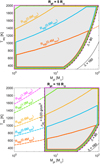 |
Fig. 1 Illustration of the criteria setting the additional boundaries on the grid (see Sect. 2.1) in the Mpl-Teq plane for 5 R⊕ (top) and 10 R⊕ (bottom) planets. The dashed orange, blue, yellow, green, and violet lines marked as RRB(M*) show the upper Teq(Mpl) boundaries set by criterion II (Rroche ≥ 1.2Rpl)forplanetsorbiting0.4, 0.6, 0.8, 1.0, and 1.3 M⊙ stars, respectively. The solid line contours of the respective colours show the grid ranges in the Teq–Mpl plane for each of the stellar masses, with all areas sharing the same lower boundary, controlled by criterion III (dashed black line for Λ = 80; dotted black line for Λ = 160). In the bottom panel, the region on the left of the shaded area (grid ranges) is excluded by the low-density criterion I (ρ ≥ 0.03 g cm−3; dash-dotted black line). |
2.2 Challenges of the grid interpolation
2.2.1 The shape of the grid boundaries in six dimensions
The inequality of the mass and radius ranges available in the grid for specific stellar masses and equilibrium temperatures, along with the limited number of grid points (which is dictated by the high computational costs of the hydrodynamic models), poses significant challenges to any grid interpolation. To outline the most problematic regions of the parameter space, panel a of Fig. A.1 shows the atmospheric mass-loss rates predicted by the hydrodynamic model for planets with radii of 5 R⊕ and masses within the grid ranges orbiting an 0.6 M⊙ star at orbital separations corresponding to Teq of 300, 700, 1100, 1500, and 2000 K as a function of Mpl. As described above, the minimum and the maximum planetary masses included in the grid are different for each Teq value (i.e. orbit), due to criterion II (minimum Rroche) and criterion III (maximum Λ), respectively. As the quality of the interpolation depends mostly on the density of grid points close to the point of interest, the shortage of points close to the grid boundaries deteriorates the quality of the prediction.
2.2.2 The switch between different escape regimes occurs across a wide parameter scale
Atmospheric escape in the different regions of the parameter space is controlled by various mechanisms and combinations thereof. For hydrodynamic mass loss, these mechanisms are defined by the dominant energy source. For high-gravity planets, the escape is typically driven by photoionisation heating (XUV- driven escape). For hot, low-gravity planets, it can be powered by the planet’s internal energy (core-powered mass loss or boil- off). In the extreme cases of planets on very short orbits (i.e. high equilibrium temperatures), the escape is driven by the stellar tidal force (Roche lobe overflow). The transition between the different regimes is illustrated in Fig. 2 and the location at which these regimes transition from one to the other (hereafter the ‘regime transition point’) can be identified by where at fixed Teq the mass-loss rate increases significantly with decreasing Mpl, Λ, or Λ × K. Here, K quantifies the relevance of tidal effects and is defined as (Erkaev et al. 2007)
 (5)
(5)
where  To better show this, we include in Fig. 2 the predictions obtained from three analytical approximations representing the three regimes. For XUV-driven escape, we considered the energy-limited mass loss (ṀEL) from Erkaev et al. (2007, dash-dotted lines), for boil-off we considered the core-powered mass-loss approximation (ṀCP) from Gupta & Schlichting (2019, solid lines), and for Roche lobe overflow (ṀRL) we considered the upper limit given by Koskinen et al. (2022, dashed lines). We describe the exact implementation of each of these approximations in detail in Appendix A.
Figure 2 shows that ṀEL describes well enough the atmospheric mass loss expected for high-gravity planets, but the mass interval in which this match is found depends strongly on Teq. For example, for the case considered in Fig. 2, at 300 K the energy-limited approximation is applicable to planets more massive than ~4M⊕, while at 700 K, 1100 K, 1500 K, and 2000 K, this boundary shifts to ~10 M⊕, ~20 M⊕, ~50 M⊕, and ~110 M⊕, respectively. Furthermore, for each temperature interval, this boundary shifts towards lower masses for higher EUV fluxes and vice versa (see details in Appendix A).
For lower-mass planets, atmospheric escape is driven mainly by a combination of the planet’s low gravity and high internal thermal energy. The shape of the line in Fig. 2 indicating corepowered mass loss comprises a steep component towards higher masses, driven by the assumption that the whole thermal energy of the planet goes into driving the escape, and a flat component, due to the limit on the mass-loss rates set by the thermal velocities of the atmospheric particles at the Bondi radius. For planets with Teq ≤ 1100 K, the transition from energy limited to core-powered mass loss occurs near the point where ṀEL ≃ ṀCP. Figure 2 shows that at low Mpl values the core-powered approximation provides just an upper limit to the atmospheric mass-loss rates, while at higher Mpl values and particularly at Teq values higher than about 1000 K (i.e. short orbital separations) stellar gravity starts driving the escape through Roche-lobe overflow (which occurs when the atmospheric pressure at the Roche lobe is as high as 10–100 nbar according to Koskinen et al. 2022). Based on the grid simulations, we find that the tidal forces driving Roche lobe overflow become non-negligible if  (i.e. K ≲ 0.7) and one of the dominant drivers if
  (i.e. K ≲ 0.3). The above estimate, however, should not be taken as an exact criterium to classify the escape, as it depends strongly on the system parameters and the assumptions of the hydrodynamic model.
To summarise, there are two regime transition points, one from XUV-driven escape to core-powered mass loss (for planets with longer orbital separations) and one from XUV-driven escape to Roche lobe overflow (for planets with shorter orbital separations). The position of the regime transition point in the Mpl dimension depends on the other system parameters, and particularly on M*, and Teq. Therefore, if the mass of the planet subject of the interpolation is close to one of the regime transition points, the interpolation can be subject to large inaccuracy, because for such planets the mass-loss rates can change significantly in response to even small variations in one of the planetary parameters, in particular for planets hotter than ~1000 K.
This problem can be eased by moving from the Ṁ–Mpl space to the Ṁ–Λ space. Therefore, instead of interpolating in the fivedimensional space {Mpl, Rpl, Teq, FEUV, M*}, one can interpolate in the five-dimensional space {Λ, Rpl, Teq, FEUV, M*}. Combining planetary mass, radius, and temperature (which, in our formulation, define the core-powered mass loss from the planet; see Appendix A for details) within one parameter allows one to significantly decrease the difference between the regime transition points from XUV-driven to core-powered mass loss at different temperatures, as shown in panel b of Fig. 2. However, this does not solve the problem for the hottest planets orbiting around low-mass stars (Teq ≥ 1500 K for 0.6 M⊙ and Teq ≥ 700 K for 0.4 M⊙), as in this case the transition goes from XUV-driven escape to Roche lobe overflow.
To overcome this last obstacle, one can employ Λ × K, instead of Λ (Guo 2024). This approach enables one to almost completely remove the difference between the two regime transition points, as shown by panel c of Fig. 2. In the Ṁ versus Λ × K space the regime transition points are located in a very narrow range and their specific position depends mainly on FEUV (they move towards lower Λ × K values for higher XUV fluxes and vice versa). This property can be used to facilitate the interpolation within the grid.
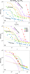 |
Fig. 2 Atmospheric mass-loss rates predicted by the hydrodynamic model for planets with Rpl = 5 R⊕ and Mpl between 1 M⊕ and 108.6 M⊕ orbiting a 0.6 M⊙ star at an orbital separation corresponding to Teq values of 300K (blue circles), 700K (green circles), 1100 K (deep yellow circles), 1500 K (violet circles), and 2000 K (red circles) as a function of Mpl (top), Λ (middle), and Λ × K (bottom). Lines of different styles indicate the mass-loss rates predicted by the energy-limited approximation ṀEL (dash-dotted), core-powered mass loss ṀCP (solid), and Roche lobe overflow ṀRL (dashed), with the colour of the lines following the same scheme as that of the circles. For ṀEL, we considered the same EUV fluxes as for the hydrodynamic models shown in the plots, namely 3.0 erg s cm−2 for the orbital separation corresponding to Teq of 300 K, 89.1 erg s cm−2 for 700K, 543.3 erg scm−2 for 1100K, 1878.6 ergs cm−2 for 1500 K, and 5937.3 erg s cm−2 for 2000 K. |
3 Test dataset
For the development of the previous interpolation algorithms (Kubyshkina et al. 2018b,a), the accuracy of the interpolation has been tested by (a) extracting about 10% of grid points from the whole sample to be then compared with the values given by the interpolation and (b) by comparing the results of the interpolation with the mass-loss rates obtained by directly applying the hydrodynamic model to a dozen real exoplanets. Although both methods have demonstrated to lead to good accuracy of the interpolation (Kubyshkina et al. 2018b), they have drawbacks. While approach (a) provides a sufficiently large test dataset, it implies that all the equilibrium temperatures and stellar host masses of the test planets are those already present in the grid, which essentially reduces the interpolation in the five-dimensional space to three dimensions, namely Mpl, Rpl, and FEUV. Approach (b), in turn, implies interpolating in the five-dimensional space, as intended, but lacks in size. Furthermore, the majority of the exoplanets observed to date are rather old, and thus fall into the part of parameter space dominated by XUV-driven mass loss (e.g. Kubyshkina 2022). Therefore, both approaches can turn out to be blind to part of the problematic parameter ranges outlined in Sect. 2.2. In this section we describe in detail the sample of simulated planets that is used to test the accuracy of the new interpolation routine described in the next section.
3.1 New test planets
To provide a more realistic estimate of the interpolation errors across the whole parameter space, we built a new test dataset using the same hydrodynamic model used to construct the grid (see Sect. 2). The test planets were set as follows. For every test planet, we first set the host star mass and equilibrium temperature at random values between 0.4 and 1.3 M⊙ and between 300 and 2000 K, respectively. From these two values, we defined the orbital separations (a = a(M*, Teq)) in the same way as for the grid planets. We then set the XUV luminosity at a random value within the limits listed in Table 1 for different stellar masses and scaled them to the fluxes at the planetary orbits using the corresponding orbital separations. Finally, for the pair of planetary mass and radius, we set Mpl at a random value between 1 and 108.6 M⊕, then using M*, Teq, a, and Mpl to define the limits for planetary radius employing Criteria I–III described in Sect. 2.1 and set Rpl at a random value within the derived limits. To set the random values, we used a uniform prior distribution, sampling in the linear space for all parameters except XUV luminosity and Mpl, which we sampled in logarithmic space. This was done so that the parameter distribution of the test sample resembles that of the grid. Furthermore, this approach ensures that planets in the XUV-driven mass-loss regime do not dominate the test sample.
After defining the set of test planets, we performed hydrodynamic modelling for each of them. Of the initial 250 models, 16 planets were excluded because the resulting atmospheres did not satisfy the hydrodynamic conditions (e.g. hydrostatic atmosphere), leaving us with a test dataset of 234 planets, which is about 2% of the entire grid and covers the grid parameter space well. Figure 3 shows the position of the test planets across the parameter space of the grid.
3.2 Grid environment of test planets
To quantify how challenging each of the test planets is in terms interpolation (see Sect. 2.2), we did the following. First, we estimated how close each test planet is to the grid boundaries to check whether, for example, the mass of the test planet is smaller (larger) than the minimum (maximum) mass among the closest grid points in terms of radius, temperature, and host star mass. Therefore, as any point in the grid can be uniquely defined by five parameters (Mpl, Rpl, FEUV, Teq, and M*), we looked for the grid points closest to each of the test planets. We then fixed four of the five parameters to (one of) these values and check if the fifth parameter range available in the grid at this condition covers that of the test planet, and repeated this procedure for different combinations of system parameters.
To express this numerically, we defined the parameter Jbord as described in Appendix B. This parameter reflects the number of cases in which one of the parameters of a test planet lies outside of the boundaries set by the closest grid points. We then normalised Jbord so that it can take a maximum value of 1, which corresponds to the situation in which a planet is outside of the grid boundaries considering all parameters. As a guidance, values of Jbord > 0.1 imply that a given test point is not covered by the grid for more than one parameter and at values above 0.15 one can expect the accuracy of the interpolation to drop significantly. For the whole test dataset, Jbord lies between 0 and 0.375 and differs from 0 for 166 points out of 234.
In addition to the test planets near the grid boundaries, we identified those lying near the regime transition points. We first located the position of the regime transition points in terms of Λ at fixed M*, Teq, Rpl, and FEUV as follows. We identified the points clearly lying in one of the three escape regimes (e.g. within the grid, mass-loss rates above 1012 g s−1 are reached just through core-powered mass loss or Roche lobe overflow, which we do not distinguish for the determination of the regime transition points). Then, we fitted linear functions through the points belonging to each of the regimes in the log Ṁ–log Λ space and set the regime transition point at the location where the lines cross (see an example in Fig. 4).
To quantify the distance in Λ space between each test point Λi and the regime transition points ΛRTP, we proceeded similarly to the case of Jbord, as described in Appendix B. For each Λi, we looked for the ΛRTP values of the nearest neighbours and introduced the parameter Jtrans, which we set equal to one if |ΛRTP – Λi|/ΛRTP < 0.2 (i.e. test point close to a regime transition point) considering any of the nearest neighbours, and to zero otherwise. Then, we looked at the points with Jtrans = 1 and re-set them to Jtrans = 2 if the difference between the minimum and maximum values of ΛRTP of the considered nearest neighbours exceeded a value of five (a situation similar to the one considered in Sect. 2.2). This was done to further highlight points located in regions of the parameter space that are more difficult to accurately interpolate.
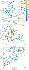 |
Fig. 3 Position of the planets comprising the test dataset in the M*– Teq plane (top), in the a–FEUV plane (middle), and in the Mpl–Rpl plane (bottom). In each panel, points are colour-coded according to the value of Λ × K (see the scale in the top panel). |
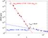 |
Fig. 4 Definition of the location of the regime transition point (ΛRTP) for M* = 0.6 M⊙, Teq = 1100 K, Rpl = 5 R⊕, and FEUV = 543.3 erg s cm−2. Grey circles show the atmospheric mass-loss rates against Λ given by the hydrodynamic model. The red asterisks denote points identified as planets in the core-powered or Roche lobe overflow regime (Ṁ ≥ 1012 g s−1 and Rroche > 1.5; the latter condition excludes points that are too much affected by the lower boundary condition). The blue crosses denote the points in the XUV-driven regime (Ṁ ≤ 109 g s−1). The red and dashed blue lines show the linear fits in the log Ṁ–log Λ space for these two groups of points, as specified in the plot. The yellow star gives the position of the regime transition point. |
3.3 Performance of the previous interpolation scheme
To roughly estimate the size of the interpolation uncertainties that one can have due to the problems described in Sect. 2.2, we calculated the atmospheric mass-loss rates (Ṁpred,21) for the planets in our test dataset using the old interpolation scheme (interpol2021; Kubyshkina et al. 2018b; Kubyshkina & Fossati 2021) and then compared them with the estimates obtained using the hydrodynamic model, which we considered here to be the ‘true’ values. The results of the comparison are shown in Fig. 5 (panels a and c). We remark that for this test we disabled the input evaluation procedure included in the distributed version of interpol2021, which would otherwise have discarded all test points with Jbord ≳ 0.1.
To gather an idea of the magnitude of the interpolation uncertainties shown in Fig. 5, we considered some of the uncertainties intrinsic to the modelling approach and resulting from some of the assumptions. Besides fundamental assumptions (e.g. hydrogen-dominated composition, cloud-free atmosphere, crosssection values), it is difficult to properly quantify the modelling uncertainties, and thus here we focused on two aspects that we believe drive most of the uncertainties, namely the assumptions on the boundary conditions and the treatment of the stellar XUV radiation. Specifically, testing indicates that for the majority of sub-Neptune-like planets in the XUV-driven escape regime on average the assumption taken to set the position of the lower boundary leads to mass-loss rate uncertainties of about a factor of 2 (see also Kubyshkina et al. 2018b, 2024), though for the most extreme planets in the grid (Λ × K ≤ 1) it can reach up to a factor of 100. For what concerns the treatment of the stellar XUV irradiation, atmospheric heating depends on the depth at which photons are absorbed, and thus on the shape of the stellar XUV spectrum, which can vary significantly from star to star. However, the grid does not take into account the specific shape of the stellar XUV emission. Furthermore, the model used to compute the grid simplifies the shape of the stellar XUV irradiation representing it in just two wavelength points (i.e. 2λ approximation; X-ray and EUV). These two simplifications affect the mass-loss predictions for most of the intermediate-mass planets (Λ × K ~ 20–50). Also in this case, the mass-loss rate uncertainties associated with these two simplifications are expected to be within a factor of 2 (e.g. Guo & Ben-Jaffel 2016; Guo 2024; Kubyshkina et al. 2022, 2024). In summary, we consider ratios of Ṁpred/Ṁtrue lying between 0.5 and 2 to be accurate predictions.
For our test dataset, in the case of interpol202l about 40% of the points (95) fall out of this range. Of them, 37 points have Jbord > 0.1 indicating that they lie near the grid boundaries in their respective parameter regions, and 61 points are close to a regime transition point (Jtrans > 0). Indeed, the majority of the test points with large interpolation errors have Jtrans = 2, and the error is maximum at the intermediate Λ values (7–40). Thus, the most problematic planets for the interpolation are hot planets orbiting low-mass stars near a regime transition point.
In an effort to improve the interpolation quality for such planets, we started by revising the previous interpolation scheme interpol2021, in which the interpolation in five dimensions (which did not provide satisfactory results for the tests described in Kubyshkina et al. 2018b) is reduced to a series of onedimensional interpolations. Furthermore, interpol2021 interpolates over the Λ values instead of planetary mass and picks one of the pair (Teq, a) as a guiding parameter depending on host star mass and temperature (Teq has a stronger impact on the mass-loss rates for cooler planets around more massive stars and a dominates for hot planets around low-mass stars).
As the new Λ × K parameter performs better than Λ at synchronising the regime transition points in different parameter intervals, we decided to switch from interpolating across Λ to interpolating across Λ × K. This allowed us to exclude a from the interpolation parameters and switch to Teq only. Furthermore, we changed the interpolation on Teq from linear to logarithmic. At last, we narrowed the criteria for picking the neighbouring points used for interpolation. We refer to this version of the interpolation routine as interpol2024 and show the testing results analogous to the case of interpol2021 (Ṁpred,24/Ṁtrue) in panels b and d of Fig. 5.
Considering the test dataset, the use of interpol2024 allowed us to reduce the total number of outliers to 45 (~20% of the test planets; 26 points correspond to Jbord > 0.1 and 18 to Jtrans > 0) and the maximum interpolation error by about 43 times, compared to interpol2021. However, there is still some systematic behaviour in the interpolation predictions, which tends to overestimate mass loss at low Λ × K values and to underestimate it at high Λ × K values. This is why we explored other interpolation algorithms, in particular, based on ML.
4 Exploring the grid interpolation in six dimensions
As described in Sect. 2.1, in the grid of hydrodynamic models the orbital separation is a function of equilibrium temperature and stellar mass. Therefore, each planet in the grid can be identified by five unique parameters {M*, FEUV, Rpl, Mpl, Teq, or a}. However, the value of the atmospheric mass-loss rate can have a stronger dependence on Teq than a in some regions of parameter space (e.g. for long-period planets), and vice versa in others (e.g. short-period planets). To take advantage of the learning abilities of ML, in the following, we are oblivious to the degeneracy between Teq and a and treat them as independent input parameters.
Considering mass-loss rates as a function of six parameters {M*, FEUV, a, Teq, Mpl, Rpl} allows one to define the relationship between these parameters and the mass-loss rate as a function f mapping from six-dimensional parameter space to one dimension space (f : ℝ6 → ℝ) in a way that y = f (x), with x ∈ ℝ6, and y ∈ ℝ. The unknown function, f, can be approximated via data-driven modelling and then applied to predict the mass-loss rate, y(q), at a new query point, x(q), such that y(q) = f (x(q)). Obtaining a numerical function from a set of data points is a high-dimensional (here, six-dimensional) non-linear regression problem that can be solved using several numerical schemes. Here, we mainly focused on two methods: traditional interpolation in the form of the radial basis function (RBF; Buhmann 2000; Powell 2001) and the ML model in the form of a NN (Hecht-Nielsen 1992; Gurney 2018; Abiodun et al. 2018; Wu & Feng 2018).
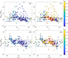 |
Fig. 5 Ratio of the mass-loss rates predicted for the test planets by interpol2021 (panels a and c) and interpol2024 (panels b and d) to the true values given by the hydrodynamic model, against Λ and Λ × K, respectively. The points are colour-coded according to the Jbord value. In panels (c) and (d), the red points have Jtrans = 1, while the red points marked by a yellow plus are those with Jtrans = 2. For reference, the two horizontal black lines in each panel lie at 0.5 and 2. |
4.1 Neural-network-based regression
We aim to design a NN architecture learning the relationship (f) between inputs x = (M*, FEUV, a, Teq, Mpl, Rpl) and output y = Ṁ. We explored several NN models, including dense neural networks (DNNs), convolutional neural networks (CNNs), and recurrent neural networks (RNNs), to train our data and evaluate prediction performance with the test data points described in Sect. 3. The DNN model, consisting of fully connected layers, is well suited for data with relatively low input and output dimensions. DNNs are effective at learning complex mappings between inputs and outputs when the relationships in the data do not require sequential processing.
Convolutional neural networks (Wu 2017; Albawi et al. 2017; Gu et al. 2018) and RNNs (Pascanu et al. 2013; Salehinejad et al. 2017) could offer better solutions with higher-dimensional data (both input and output data are high-dimensional arrays). Convolutional layers in a CNN model extract features from higher-dimensional data, which helps extract hidden features. Since our data do not require extracting hidden features, adding a convolution layer to the input layer is not advantageous. In fact, our tests showed that CNN-based predictions of mass-loss rates from six-dimensional grid points deviated significantly from the actual values, aligning with expectations for CNN performance in cases like ours.
The RNNs, including variants such as long short-term memory (LSTM; Hochreiter & Schmidhuber 1997) networks, are specific types ofNN models, where the input of the current layer is connected to the output of the previous one. This allows the model to create a memory through a chain of relations between the input and output of the hidden layers. Thus, RNN models help us better forecast specific kinds of data, such as time series. Although RNNs can predict mass-loss rates with accuracy comparable to DNNs under specific configurations, they come with a higher computational cost due to the increased number of trainable parameters. Furthermore, RNNs require significantly larger training datasets to outperform DNNs in scenarios like ours. The mass-loss rate prediction obtained using a simple RNN and LSTM model is shown in Appendix D.
Since CNNs and RNNs have more trainable parameters than DNNs, they require significantly larger training datasets to achieve better prediction quality. Furthermore, the simplicity and the ability to generalise well from limited datasets allow DNNs to achieve better prediction accuracy than advanced and complex models like CNNs or RNNs, making DNNs an optimal choice. Given the training dataset size and the nature of the parameter space, the DNN model offers superior prediction accuracy, making it the most suitable choice for our analysis. Hence, our work mainly focused on DNN-model-based prediction.
A DNN is a simple NN architecture with dense (fully connected) layers. It is one of the primary and fundamental architectures in deep learning for solving linear and non-linear regression problems. In this type of network, each neuron in a layer is connected to every neuron in the subsequent layer. The network typically consists of an input layer, one or more hidden layers, and an output layer (see Fig. 6). The input layer receives the data, and each hidden layer processes these data by applying a linear followed by a non-linear transformation. The linear transformation of the data is done through weights and biases, while the non-linear transformation is obtained via the activation function (Narayan 1997; Sibi et al. 2013; Sharma et al. 2017; Ramachandran et al. 2017). The activation function can, for example, be a Sigmoid, a rectified linear unit (ReLU), an exponential linear unit (ELU), a Tanh. Transforming the whole training input data through linear–non-linear transformation is called forward propagation. The output layer provides the final predictions, with the number of neurons in this layer corresponding to the number of prediction regression targets (in our case, the single parameter Ṁ). The loss function measures the correctness of the projections. For the regression problem, the loss is usually defined as the mean-squared error between predicted and true values. With initial epochs of NN training, the loss is expected to be high. Hence, during training, the network updates weights and biases via back-propagation and gradient descent, which minimises the loss function. Despite its simplicity, a network with dense layers can capture complex patterns in the data, making it a powerful tool for solving non-linear regression problems.
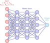 |
Fig. 6 Schematic representation of a DNN architecture connecting the input parameters and mass-loss rate (output) through a series of hidden layers. In this work, we finally opted for three hidden layers and eight neurons. |
4.2 Radial-basis-function-based regression
The regression problem can also be solved through traditional interpolation methods such as Chebyshev polynomials and the RBF. Chebyshev polynomials require a fixed grid structure for interpolation, whereas the RBF is a mesh-free method. Due to the mesh-free nature of the RBF method, the number of interpolation nodes can be scaled with increasing dimensions of the parameter space. Hence, RBF-based regression is suitable for high-dimensional interpolation with a small or limited number of nodes, which is the case for our grid of hydrodynamic models. The number of required nodes for Chebyshev’s polynomial scales exponentially with increasing dimension number of the parameter space, which increases computational costs. Hence, we restricted ourselves to exploring the regression problem with RBF only. Mathematically, an unknown function between a given set of input x and output y can be written as a linear combination of N-specific radial basis and unknown weights:
 (6)
(6)
where {wi, i = 1, 2, ⋯, N} are the adjustable weights (or coefficients) and {Φi} are the RBFs, which depend on the distance between the input x and a centre xi. Equation (6) shows that in an RBF-based regression problem, the given input data {xi} are transformed using RBF-basis (kernel), which can be represented by known functions (e.g. linear and Gaussian). Hence, the regression problem boils down to an optimisation in which we need to optimise the corresponding unknown weights of the RBF basis.
5 Application to the grid of upper atmosphere models
The treatment of RBF and NN models for performing regression tasks differs significantly due to their inheritance structure of the solution schemes. A NN is a ML method that involves training and testing stages, which typically means that the available data (in our case, grid points) is split into training and testing subsets (e.g. 90% vs. 10% of the points) and only the former is used to optimise the solution. Meanwhile, in RBF a system of equations is solved to obtain the optimised weights without splitting the data between training and testing. However, to compare the performance of the models, we used the entire grid points in both cases, namely to train the NN model or to obtain optimal weights of radial basis, and employed the test dataset described in Sect. 3 to test the performance of both a NN and a RBF.
The results obtained for the old interpolation scheme indicate that the form we use to represent the basic input parameter can affect the results. Therefore, we explored several parameter combinations to solve the regression problem using a NN and a RBF. Along with the usual six-dimensional parameter space with {M*, FEUV, a, Teq, Mpl, Rpl}, we tried to solve the regression problem using other combinations, including
parameter space reduced to five dimensions by excluding Teq or a,
six-dimensional parameter space, but with Mpl replaced by Λ or Λ × K,
parameter space extended to seven dimensions, including both Mpl and Λ or Λ × K.
and combinations thereof. We find that solving the regression problem with the six-dimensional input parameters {M*, FEUV, a, Teq, Λ × K, Rpl} (namely with Λ × K replacing Mpl) predicts the mass-loss rate better for the test dataset compared to other options.
For the training procedure of the DNN model, we used the entire grid, namely 11 442 points. The input variables Teq and FEUV were taken on a base-10 logarithmic scale. The mass-loss values are taken as base-10 logarithmic values and normalised such that max (log10(Ṁ)) = 1 by applying the MinMaxScaler scale. Therefore, the final prediction of the DNN is between zero and one, and we performed two reverse transformations to obtain the final prediction in the original scale.
Due to the limited training dataset, investigating the correct choice of a NN architecture is crucial to avoid overfitting and achieve a good generalised functional form. Overfitting occurs when the DNN has too many trainable parameters (such as weights and biases), enabling it to fit the training data closely, but resulting in poor performance on unseen test data (Hinton 2012). Conversely, a model with fewer parameters can lower the risk of overfitting, but it must retain sufficient capacity to capture meaningful information, ensuring it generalises effectively to new data. The parameters for each dense layer are calculated based on the number of input units, weights, and biases. For example, in this problem, six is the dimension of the input vector, and ℓ is the number of neurons. There will be a weight matrix of size 6×ℓ and ℓ number of biases. Thus, the parameters between the input layer and the first hidden layer are 7ℓ (= 6 × ℓ + ℓ). Similarly, the number of trainable parameters between the first and second hidden layers is 9ℓ (= 8 × ℓ + ℓ). Hence, the total number of trainable parameters (NTP) for a fully connected DNN is
 (7)
(7)
where m and n are the numbers of input and output units for each layer, respectively, and hk is the number of hidden layers. The plus one term is to include the bias terms. Equation (7) indicates that many hidden layers and a large number of neurons increase the number of total trainable parameters that, in turn, increase the complexity of the problem, and more training data would be needed. For simplicity, we began with a lighter DNN architecture (e.g. a single hidden layer), gradually increased complexity in terms of the number of layers (up to 10) and neurons (up to 512; see Appendix D), and obtained prediction accuracy on the test dataset for each architecture. The training of the models has been carried out for a maximum of 5000 epochs, with a learning rate of 10−4 and batch size of 32. Out of all variations, we find that three layers of DNN architecture with tanh activation function and eight neurons provide the best prediction accuracy on the unseen test data (described in Sect. 3), as shown in Fig. 7.
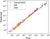 |
Fig. 7 Mass-loss rate values predicted by the DNN (dark yellow), RBF (magenta), and interpol2024 (blue) schemes in comparison to the true values obtained from the hydrodynamic modelling for the test dataset. The prediction accuracy of the DNN, RBF, and interpol2024 schemes are roughly comparable (see Sect. 6) and outperform those of interpol2021. |
6 Validation of the new approach
To test the effectiveness of the trained DNN and RBF models, we used the test dataset of 234 planets described in Sect. 3, which is unknown to the trained model (i.e. input grid). We computed the ratio between actual and interpolated mass-loss rates considering the DNN and RBF methods. The left panel of Fig. 8 shows the histogram of this ratio, which is expected to be around one if the interpolation matches the actual value. For the DNN and RBF, the peak of the histogram is nearly at one, showing that for most of the test dataset the interpolation is reasonable. For both models, the largest ratio is of order five and is found for a specific point only, while, for most of the points, the ratio lies between 0.5 and 2.
The right panel of Fig. 8 shows the fraction of points having the mass-loss rate ratio in the 0.1–10 range. The number of points lying in this ratio range is ~92%, ~83%, and ~78% for the DNN, RBF, and interpol2024, respectively, reflecting the better performance of a DNN over the other two methods. Appendix C describes in detail the RBF kernel optimisation that has been carried out.
Figure 9 further describes the quality of the interpolation for the points comprising the test dataset as a function of the interpolation algorithm. The DNN leads to the smallest number of points in which the interpolated value lies away from the true value by more than a factor of 2. As expected, these points are located at the edges of the grid in terms of mass-loss rate and close to the regime transition points. Therefore, future grid extensions should also focus on increasing the number of points in these regions of the parameter space, which will then lead to improve the quality of the DNN interpolation.
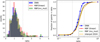 |
Fig. 8 Distribution of the mass-loss rate ratio between interpolated and true values for the test dataset. Left: Ratio between interpolated and true values for the test dataset using the DNN (blue), the RBF with a linear kernel (red), and the RBF with a inverse_multiquadratic kernel (green). For the DNN, ~92% of the points have ratios lying between 0.5 and 2, while for RBF and interpol2024 (not shown for better visualisation) it is ~83% and ~78%, respectively. Right: Cumulative distribution of the fraction of points having the mass-loss rate ratio in the 0.1–10 range. DNN interpolation outperforms the other methods. The RBF interpolation with linear and inverse_multiquadratic (inv_mul) are nearly identical. The choice of shape parameter ϵ and degree of polynomials are different and have been obtained via a grid-based optimisation process, as described in Appendix C. |
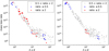 |
Fig. 9 Mass-loss rate of the test dataset as a function of Λ × K considering the RBF (left) and DNN (right) interpolation algorithms. The points for which the ratio between the interpolated and true mass-loss rates is smaller than 0.5 or larger than 2 are highlighted in red and blue, respectively. |
7 MLink: atmospheric Mass Loss INquiry frameworK
We provide public access to the trained neural network and RBF models1, allowing users to directly predict a mass-loss rate without training the model from scratch. The NN has been trained using the TensorFlow library and saved in the HDF5 format, which is compatible with TensorFlow’s load_model function. Users can load the pre-trained model into their environment to predict outcomes on new datasets with minimal setup. This functionality is included in both command-line and plug-in versions, ensuring users can leverage the predictive capabilities of the model in their preferred workflow. Detailed instructions for loading and using the pre-trained model are provided in the documentation, ensuring a smooth and efficient user experience.
Command-line version: This version allows users to run the model directly from the command line, making executing the testing processes straightforward.
Plug-in version: This version is tailored for integration within a user-defined modelling framework (e.g. the atmospheric evolution model described in Sect. 8). It includes additional functionality to interface with an external code, allowing the model to adapt dynamically and evolve based on incoming data. This version is designed with modularity in mind, ensuring it can integrate into existing systems.
8 Impact of improved accuracy on exoplanetary evolution calculations
Atmospheric evolution modelling requires re-estimating the atmospheric mass-loss rates thousands of times throughout the planetary lifetime, which, due to its fast computation, is the ideal application test-bed for the new interpolation scheme presented above (see e.g. Kubyshkina et al. 2019, 2020; Bonfanti et al. 2021; Affolter et al. 2023). Furthermore, the impact of inaccuracies in the estimation of the mass-loss rates is expected to accumulate in presence of systematic errors. In this section we use the atmospheric evolution framework developed by Kubyshkina et al. (2020) and Kubyshkina & Fossati (2022) to present tests of how different interpolation schemes affect the planetary evolutionary tracks. To complete the picture, we compared the evolutionary tracks obtained using interp2024 and MLink to those obtained using the analytical approximations commonly employed to estimate the atmospheric mass-loss rates (energy-limited equation and core-powered mass loss, as described in Appendix A). In particular, we employed the evolution model from Kubyshkina & Fossati (2022), which is based on the earlier framework by Chen & Rogers (2016) and combines the thermal evolution of planets (lower atmosphere structure models) performed with Modules for Experiments in Stellar Astrophysics (MESA; Paxton et al. 2011, 2013, 2015, 2018) code with the atmospheric mass loss at the upper boundary prescribed by MLink, interpol2024, or one of the analytical approximations.
We considered planets in the Neptune-like range of masses (initial masses  of 5 M⊕, 9 M⊕, 17 M⊕, and 30 M⊕) evolving in orbits corresponding to the temperature range 500–1700 K (where the atmospheric escape is significant and, hence, the impact of mass loss is largest) around stars of 0.5, 0.7, and 0.9 M⊙. The temperature and stellar mass values correspond to the parameter regions where the interpolation errors of our method are expected to be largest. For the initial atmospheric mass fractions
  , we employed the values predicted by the analytical approximation of Mordasini (2020) for planets of the given temperature orbiting a Sun-like star. Table 2 gives the full list of considered planets. For illustration purposes, we include an extra model identical to model 23, but with an initial atmospheric mass fraction twice as large as that predicted by Mordasini (2020). To model the evolution of the host stars, we employed the stellar evolution code Mors (Johnstone et al. 2021; Spada et al. 2013) and assumed that the stars are moderate rotators, namely we set the rotational periods of all stars to be 6 days at the age of 150 Myr.
For each simulation, we let the planet evolve for 10 Gyr or until the atmosphere is fully evaporated (i.e. atmospheric mass fraction equal to zero). As an example, Fig. 10 shows the evolutionary tracks of three highly irradiated planets: a 9 M⊕ planet orbiting an 0.5 M⊙ star at 0.0151 AU (i.e. Teq ≃ 1000 K; simulation 22 in Table 2), a 17 M⊕ planet orbiting an 0.5 M⊙ star at 0.0151 AU and starting its evolution with  set to be twice of what predicted by approximation given in Mordasini (2020, i.e. Teq ≃ 1000 K; simulation 25 in Table 2), and of a 30 M⊕ planet orbiting an 0.7 M⊙ star at 0.0113 AU (i.e. Teq ≃ 1700 K; simulation 16 in Table 2). For all planets, lines of different colours show the tracks predicted using different atmospheric escape models as detailed in the legend.
In all cases, the MLink and interpol2024 predict similar escape rates, and thus similar evolution of planetary radii. We have already shown in Sect. 2.2 that the energy-limited approximation can drastically underestimate the escape from low-mass puffy planets (see also Krenn et al. 2021, which is the case for model 25). For more compact planets (in particular, highly irradiated ones with FEUV > 104 erg s cm−2), it can instead overestimate the escape as it ignores radiative recombination and losses (e.g. Murray-Clay et al. 2009; Kurokawa & Nakamoto 2014, this is the case for models 16 and 22). For all planets in Fig. 10, the EUV flux exceeds 105 erg s cm−2 at the beginning of the evolution, and thus the energy-limited approximation leads to atmospheric lifetimes of ~6 (for the 9 M⊕ planet, model 22) and ~10 (for the 30 M⊕ planet, model 16) shorter compared to the hydrodynamic model (i.e. MLink and interplol2024). For both models 16 and 22, the atmosphere evaporates completely before ~1 Gyr; therefore, this inaccuracy of the energy-limited prescription does not play a role in shaping the predicted massradius distribution of this kind of planet at the ages of a few billion years. However, it can be essential for adequately studying young planetary systems.
Instead, the core-powered mass-loss approximation tends to underestimate atmospheric loss for compact planets on long timescales. Thus, for the 9 M⊕ planet in Fig. 10, the corepowered mass loss at the beginning of the simulation is about an order of magnitude above the prediction of both MLink and interpol2024. However, due to the planet contraction and decline of Teq, the strong escape ceases within a few tens of megayears and ṀCP does not exceed 1010 g s−1 after 100 Myr. Therefore, the planet preserves its atmosphere until the end of the simulation. For the 30 M⊕ planet, despite its higher Teq, core-powered mass loss remains negligible (~ 1000 times lower than that predicted by hydrodynamic modelling) throughout the evolution and the final radius resembles the one that would be obtained without considering atmospheric escape. Finally, the right panel of Fig. 10 shows that combining energy-limited and core-powered mass-loss rates also does not necessarily lead to reproduce what predicted by hydrodynamic models.
In the top panel of Fig. 11, we examine the performance of the MLink and interpol2024 interpolations by comparing the positions of the model planets 1–24 in the mass-radius diagram at the age of 5 Gyr. For better visualisation of the results, we plot the radii against the planetary masses normalised to the masses of their hosts. One can see that, despite some localised differences in the escape rates, the two methods predict, in general, very similar planetary parameters at ages of billions of years. However, for some planets, the difference in the predicted radii exceeds the typical observational uncertainties of ~5%, and remarkably these are the planets located close to the boundary between planets that preserve their primordial atmosphere and those that lose it (i.e. planets close to the radius gap; the largest difference among our test planets is achieved for models 7 and 12). This highlights the importance of accurate mass-loss determination in studying phenomena such as the radius gap and the hot Neptune desert.
The bottom panel of Fig. 11 matches the predictions of the MLink with those of the analytical approximations. The energy-limited approximation (in the formulation described in Appendix A) is accurate for planets under moderate conditions, but fails for planets near the radius gap (see e.g. model planets 12, 17, and 24). For the core-powered mass loss, for which we only show the models where the escape rates exceed 105 g s−1, we find that it tends to overestimate the planetary radii, particularly for planets near the radius gap.
Finally, Fig. 12 compares the atmospheric evaporation timescales between the MLink and interpol2024 for planets that fail to preserve their primordial atmospheres. We find comparable results between the two interpolation methods and differences become noticeable for planets with Teq ~ 1000 K orbiting stars of 0.7 M⊙ and 0.9 M⊙ (i.e. planets losing their atmospheres at a moderate pace).
Parameters of the planets employed to test the impact of different mass-loss prescriptions on atmospheric evolution.
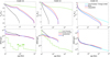 |
Fig. 10 Planetary radius (top) and mass-loss rate (bottom) evolutionary tracks for planets 16 (left; M* =0.7 M⊙; Teq = 1700K; a = 0.0113 AU; |


9 Summary and concluding remarks
The mass-loss rates of planets with hydrodynamic atmospheres depend on many parameters in a non-linear way, and their values can span as much as ten orders of magnitude. Therefore, estimating the atmospheric mass-loss rates for a given planet is a non-trivial task that in general requires the use of elaborated hydrodynamic models at large computational costs, precluding their use in planet population and evolution studies, and thus forcing one to employ (over-)simplified analytical approximations. This problem can be overcome by employing a large grid of pre-calculated upper atmosphere models, further interpolating among them (Kubyshkina et al. 2018b,a; Kubyshkina & Fossati 2021). However, accurate interpolation within the grid remains a challenging task.
The interpolation scheme developed in our earlier works (see Kubyshkina et al. 2018b; Kubyshkina & Fossati 2021) has allowed for a significant improvement over commonly employed analytical approximations (e.g. Krenn et al. 2021). However, it is still subject to significant interpolation errors in some specific regions of the parameter space. To overcome this problem, we introduced a new interpolation approach, called MLink, based on a DNN ML scheme to estimate mass-loss rates from the existing grid of hydrodynamic upper atmosphere models. This new approach led to a more reliable interpolation, which has improved the quality of the mass-loss estimates over previous methods.
We tested the new interpolation method by studying the evolution of a small sample of planets with parameters chosen in such a way as to maximise the impact of interpolation errors. To model atmospheric evolution, we employed the framework developed in Kubyshkina et al. (2020) and Kubyshkina & Fossati (2022) and performed the modelling for a range of Neptune-like planets with masses in the 5-30 M⊕ range in different orbits and around different stellar hosts. We find that for most cases, MLink and the old mass-loss interpolation schemes lead to comparable planetary parameters on gigayear timescales, though the evolutionary paths can be slightly different during some parts of the evolution. Furthermore, we find that for some planets, particularly those at the top edge of the radius gap, the difference between the predicted planetary radii at a given age of tracks obtained with MLink and classical interpolation schemes can exceed the typical observational uncertainties.
Our results clearly indicate that ML can be successfully used to estimate atmospheric mass-loss rates from a model grid. This paves the way to the exploration of future larger and more complex grids of models that will have to be computed accounting for more physical processes, such as different atmospheric compositions or the impact of various photospheric conditions at the lower boundary (e.g. the presence of aerosols).
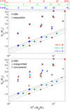 |
Fig. 11 Mass–radius distribution at 5 Gyr as predicted by the evolution model for synthetic planets 1–24 employing different atmospheric mass-loss models. Top: comparison of MLink (stars) with interpol2024 (circles). Bottom panel: comparison of MLink with energy-limited approximation (squares) and core-powered mass loss (diamonds). In both panels, the symbol fill colour indicates the equilibrium temperature of the planet (red for 500 K, turquoise for 1000 K, and blue for 1700 K), and the contour line of the symbols indicates the mass of the host star (blue line for 0.9 M⊙, green for 0.7 M⊙, and red for 0.5 M⊙). To ease the comparison, the masses of the planets are normalised to the mass of their host stars, but the three x-axes at the top give the scale in Earth masses for each considered stellar mass. The three black lines, show the radius corresponding to the bare rocky core as a function of the host star mass (solid for 0.9 M⊙, dashed for 0.7 M⊙, and dash-dotted for 0.5 M⊙). |
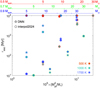 |
Fig. 12 Comparison of the atmosphere evaporation time, τesc, between the evolutionary models employing MLink (stars) and interpol2024 (circles). τesc is shown against the planetary initial mass normalised to the host star mass, but the three x-axes at the top give the scale in Earth masses for each considered stellar mass. The symbol fill colour and contour are the same as in Fig. 11. |
Acknowledgements
D.K. was supported by a Schrödinger Fellowship supported by the Austrian Science Fund (FWF) project number J4792 (FEPLowS). We thank the anonymous referee for their comments that helped improving the presentation of the results.
Appendix A Relation of hydrodynamic model predictions to common analytical approximation
In different regions of the parameter space, hydrodynamic escape can be driven by photoionisation heating (XUV-driven escape), the own thermal energy of a planet (core-powered mass loss or boil-off), tidal forces of the host star (Roche lobe overflow), or their combination. To help us understand which of the mechanisms is dominant for a specific planet, it is convenient to compare the predictions of hydrodynamic models to analytic approximations parameterising each of these processes separately.
A.1 Energy-limited approximation
For XUV-driven escape, we considered the energy-limited approximation (see the dash-dotted lines in Fig. A.1)
 (A.1)
(A.1)
where η is the heating efficiency quantifying the fraction of the total stellar energy absorbed in the atmosphere transformed into heating, G is the gravitational constant, and K is the parameter quantifying the effect of stellar tidal forces (see our Eq. 5 and Erkaev et al. 2007). The effective radius of EUV absorption (located somewhat above the photosphere) was taken according to the approximation (Chen & Rogers 2016)
 (A.2)
(A.2)
where H is the atmospheric height scale normalised to the planetary radius
 (A.3)
(A.3)
PEuv estimates the pressure at the EUV absorption level
 (A.4)
(A.4)
 is the planetary gravitational potential, kb is the Boltzmann constant, and σ20 eV is the absorption cross-section of photons with energy of 20 eV. The photospheric pressure Pphoto was set to the values employed for the lower boundary of the simulation domain in the hydrodynamic models (Eq. 1).
A.2 Core-powered mass loss
To assess how the predictions of the hydrodynamic models compare with the core-powered mass-loss approximation, we followed the approach of Gupta & Schlichting (2019) and made the following assumptions. First, we assumed that the atmospheres have solar metallicity (Z* = 1) and behave as an ideal gas (adiabatic index γ = 5/3). We also assumed that the mean weight of the atmospheric species is approximately the weight of molecular hydrogen (2mH) at the planetary photosphere and the weight of atomic hydrogen (mH) at high altitudes (e.g. at the sonic point/Bondi radius). For the radius of the planetary core (i.e. solid part of the planet composed of rocks and metals), we adopted the approximation (Rogers & Seager 2010)
 (A.5)
(A.5)
and assumed that the core mass (Mcore) is approximately equal to Mpl. Both assumptions on the core parameters have a minor impact on the results. Differently from the hydrodynamic models, here gravity is defined at the core radius, namely  .
.
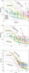 |
Fig. A.1 Same as Fig. 2, but with more FEUV values. Multiple dash-dotted lines of the same colour show the predictions of the energy-limited approximation for different FEUV values, and the multiple sequences of circles of the same colours give the predictions of the hydrodynamic model for the corresponding FEUV values (which coincide for the low-gravity planets). The considered EUV emission values are (from the bottom to the top line or sequence of each colour): 3.0, 375.5, and 3000 erg s cm−2 for 300 K; 2.6, 89.1, and ~1.1 × 10⁴ erg s cm−2 for 700 K; 16, 193.6, 543.3, and ~6.8 × 10⁴ ergs cm−2 for 1100 K; 55.4, 669.6, 1878.6, and ~2.35 × 10⁵ erg s cm−2 for 1500K; 175.2, 5937.3, and ~7.4 × 10⁵ erg s cm−2 for 2000 K. |
Furthermore, Gupta & Schlichting (2019) assume that the radiative-convective boundary (RCB) coincides approximately with the visible radius (RRCB ≃ Rpl, which might not be strictly accurate for puffy sub-Neptunes). In this case, the temperature at the RCB can be assumed to be TRCB ≃ Teq (assuming zero albedo, as for the grid planets), and for the pressure at the RCB (PRCB) one can employ the values predicted by Eq. 1. Therefore, the parameters adopted for the RCB are identical to the lower boundary parameters of the hydrodynamic models. Then, the density at RCB can be computed as
 (A.6)
(A.6)
The sonic velocity at the photosphere is  , and thus under the assumption of isothermal atmosphere the sonic point can be estimated as
 (A.7)
(A.7)
The modified Bondi radius (Ginzburg et al. 2018) is
 (A.8)
(A.8)
and the opacity at the RCB is given by the approximation (Freedman et al. 2008; Lee & Chiang 2015)
 (A.9)
(A.9)
Following these assumptions and considerations, the cooling luminosity of a planet can be estimated as
 (A.10)
where σSB = 5.6704 × 10⁻⁵ erg cm−2 s−1 K−4 is the Stefan- Boltzmann constant. Assuming the entire cooling luminosity goes into driving the escape, the mass loss powered by the core luminosity is
 (A.11)
This value is further restricted by the mechanical limit on the atmospheric mass-loss rate set by the thermal velocity of the gas molecules at the Bondi radius, which is considered to be approximately equal to that at the sonic point (Ginzburg & Sari 2016, Bondi-limited mass loss),
 (A.12)
The actual core-powered mass-loss rate ṀCP is then given by the minimum of the two mass-loss rates ṀCL and ṀBL.
A.3 Roche lobe overflow limit
To roughly estimate mass-loss rates due to atmospheric disruption by stellar tidal forces, we modified the analytical expression of Koskinen et al. (2022). The original formulation quantifies the mass-loss rate through scaling based on the difference in the gravitational potentials between the Roche lobe and the exobase. However, in general, one needs to employ hydrodynamic modelling to know the position and other parameters of the exobase. To overcome this uncertainty, we used the difference between the Roche lobe and the photosphere, which is also indicative of the effect of stellar gravity on a planetary atmosphere (as was used to derive K; Erkaev et al. 2007). In this way, atmospheric mass loss due to Roche lobe overflow can be approximated as
 (A.13)
where the first part of the expression on the right hand side quantifies the mass flow through the photosphere, if it would occur with sonic velocity Cs0 (which is close to reality in extreme cases), and Groc is proportional to the difference in gravitational potential Ur between the photosphere and the Roche lobe,
 (A.14)
with the gravitational potential accounting for the gravitational forces of the planet and of the host star, and for the orbital motion
 (A.15)
Finally,  in Eq. A.13 accounts for the deviation of the equipotential surface from spherical form: it is the distance in polar direction z where the gravitational potential Uz becomes equal to Ur(Rpl), where
 (A.16)
Equation A.13 overestimates the escape for the majority of planets, as it assumes that the atmospheric outflow occurs with a speed close to the sonic velocity already at the photosphere, while for a typical planet in the XUV-driven regime within our grid the outflow velocity at the photosphere is close, or equal, to zero. However, it can reproduce some of the most extreme points in the grid (hot puffy planets with Rroche ≲ 1.8 Rpl.
Appendix B Quantifying the quality of data coverage
We first defined the parameter differences between test points and the nearest neighbouring grid points, hierarchically, starting from M*, and proceeding with Teq, FEUV, and Rpl. For a test point with parameters  , we first defined the two stellar masses in the grid where
  is the smallest. Typically,
  is located between the two grid values
  and
and  . We then considered all the Teq values available in the grid for
  and
and  and introduced the parameter
  , with j = 1,2, setting it equal to 0, if
  is between the maximum and the minimum temperature available for
  and setting it equal to 1 otherwise. Then, for each
  and
and  , we defined the two equilibrium temperatures closest to
  , obtaining four differences between the test point i and the nearest neighbouring grid points in terms of
  . The differences in terms of a are the same, as Teq and a are directly linked. For each
  , with k = 1,2, we considered the range of available FEUV values and defined
  similarly to
  . Similarly, we considered the FEUV values closest to
  for each pair of
  and
and  , obtaining eight differences between the test point i and the nearest neighbouring grid points, and proceeded in the same way for Rpl for each pair of
  , and
, and  , obtaining 16 differences between the test point i and the nearest neighbouring grid points, and thus defining
  and
and  . Finally, similarly to
  we defined its analogue in terms of orbital separation
  , and similarly to
  we defined the Jbord parameters based on Λ and Λ × K
  . At last, we computed the cumulative Jbord value as
 (B.1)
(B.1)
Appendix C Optimisation on RBF kernels
We comprehensively explored the available kernel options in the ‘RBFInterpolator’ function of the SciPy package. These kernels include linear, gaussian, cubic, thin_plate_spline, quintic, multiquadric, inverse_multiquadric (inv_mul), and inverse_quadratic. We used a grid-based search approach to optimise the shape parameter (є) and the degree of the polynomial (d) where applicable. We defined a grid of values for each kernel to test the shape parameter and polynomial degrees within a suitable range. The polynomial degrees for applicable kernels have been varied between 1 and 4.
The ranges of shape parameters varied depending on the kernel due to their differing mathematical characteristics. For instance: (a) For the quintic kernel, we tested є values from the grid [0.01,0.02,0.1,0.2,0.3,1.0,2.0,3.0,5.0,10.0]. (b) The shape parameter does not considerably influence the smoothing behaviour for the linear kernel. However, for a thorough investigation, we evaluated a range of values [0.1,0.2,0.3,0.4,0.5,0.6,1.0,2.0, 3.0,5.0,10.0]. After a grid search, we found that the best shape parameter value was 1.0, aligning with theoretical expectations. Table C.1 shows the optimised values of є and d for each kernel.
Except for quintic and gaussian, all kernels (linear, cubic, thin_plate_spline, multiquadric, inverse_multiquadric, and inverse_quadratic) exhibited nearly similar accuracy with the test data. Despite the optimised kernel choice, none of these kernels outperformed the accuracy of the three-layer NN, indicating that the DNN achieves slightly better accuracy than other RBF kernels for the test dataset.
Optimised є and d values after a grid-based search.
Appendix D LSTM network
The DNN model captures the mass-loss rate calculation using six input parameters. Also, we explored LSTM networks for the same task. LSTM, a specialised RNN, uses cell states, hidden states, and gating mechanisms to process sequential data and produce continuous outputs (Hochreiter & Schmidhuber 1997). The model includes one LSTM layer with 50 units, designed to handle input sequences of shape (1,6), corresponding to singletime steps with six features, followed by a dense output layer generating a continuous output. Figure D.1 shows the model’s predictions. Multiple LSTM layers can be stacked to enhance performance, improving accuracy with more extensive grid data. We explored deeper DNN architectures with additional layers (e.g. 10) and neurons (e.g. 512) or more complex Dense LSTM models as more comprehensive grids become available. We remark that a ten-layer DNN or LSTM architecture has the potential to achieve superior accuracy when trained with more extensive grid data, making them promising starting points for developing future advanced models. Meanwhile, the three- layer DNN and RBF models outperform the previously proposed method for the current training and testing dataset.
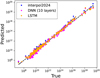 |
Fig. D.1 Mass-loss rates predicted using the LSTM (dark yellow), DNN (magenta), and interpol2024 (blue) schemes, compared to the actual values obtained from the hydrodynamic modelling for the test dataset. The LSTM architecture consists of a single LSTM layer with 50 units, while the DNN comprises ten hidden layers with 512 neurons each. The DNN architecture is significantly more complex than the LSTM, resulting in approximately 2.63 million trainable parameters for the DNN compared to around 11,500 for the LSTM. This heavier model impacts the DNN’s overall accuracy, making it less accurate than the LSTM due to overfitting (Hinton 2012). However, with an extended dataset, it is expected that the DNN would perform better on unseen test data. |
References
- Abiodun, O. I., Jantan, A., Omolara, A. E., et al. 2018, Heliyon, 4, e00938 [CrossRef] [PubMed] [Google Scholar]
- Affolter, L., Mordasini, C., Oza, A. V., Kubyshkina, D., & Fossati, L. 2023, A&A, 676, A119 [NASA ADS] [CrossRef] [EDP Sciences] [Google Scholar]
- Albawi, S., Mohammed, T. A., & Al-Zawi, S. 2017, in 2017 International Conference on Engineering and Technology (ICET) (IEEE), 1 [Google Scholar]
- Benz, W., Broeg, C., Fortier, A., et al. 2021, Exp. Astron., 51, 109 [Google Scholar]
- Bonfanti, A., Fossati, L., Kubyshkina, D., & Cubillos, P. E. 2021, A&A, 656, A157 [NASA ADS] [CrossRef] [EDP Sciences] [Google Scholar]
- Bonfanti, A., Brady, M., Wilson, T. G., et al. 2024, A&A, 682, A66 [NASA ADS] [CrossRef] [EDP Sciences] [Google Scholar]
- Buhmann, M. D. 2000, Acta numerica, 9, 1 [CrossRef] [Google Scholar]
- Carleo, I., Gandolfi, D., Barragán, O., et al. 2020, AJ, 160, 114 [Google Scholar]
- Chen, H., & Rogers, L. A. 2016, ApJ, 831, 180 [Google Scholar]
- Choi, J., Dotter, A., Conroy, C., et al. 2016, ApJ, 823, 102 [Google Scholar]
- Cubillos, P. E., Fossati, L., Erkaev, N. V., et al. 2017, ApJ, 849, 145 [NASA ADS] [CrossRef] [Google Scholar]
- Erkaev, N. V., Kulikov, Y. N., Lammer, H., et al. 2007, A&A, 472, 329 [NASA ADS] [CrossRef] [EDP Sciences] [Google Scholar]
- Fossati, L., Erkaev, N. V., Lammer, H., et al. 2017, A&A, 598, A90 [NASA ADS] [CrossRef] [EDP Sciences] [Google Scholar]
- Freedman, R. S., Marley, M. S., & Lodders, K. 2008, ApJS, 174, 504 [NASA ADS] [CrossRef] [Google Scholar]
- Gandolfi, D., Fossati, L., Livingston, J. H., et al. 2019, ApJ, 876, L24 [Google Scholar]
- Ginzburg, S., & Sari, R. 2016, ApJ, 819, 116 [NASA ADS] [CrossRef] [Google Scholar]
- Ginzburg, S., Schlichting, H. E., & Sari, R. 2018, MNRAS, 476, 759 [Google Scholar]
- Gu, J., Wang, Z., Kuen, J., et al. 2018, Pattern Recognit., 77, 354 [CrossRef] [Google Scholar]
- Günther, M. N., Pozuelos, F. J., Dittmann, J. A., et al. 2019, Nat. Astron., 3, 1099 [Google Scholar]
- Guo, J. H. 2024, Nat. Astron., 8, 920 [NASA ADS] [CrossRef] [Google Scholar]
- Guo, J. H., & Ben-Jaffel, L. 2016, ApJ, 818, 107 [Google Scholar]
- Gupta, A., & Schlichting, H. E. 2019, MNRAS, 487, 24 [Google Scholar]
- Gurney, K. 2018, An Introduction to Neural Networks (CRC press) [CrossRef] [Google Scholar]
- Hadden, S., & Lithwick, Y. 2017, AJ, 154, 5 [Google Scholar]
- Hecht-Nielsen, R. 1992, in Neural Networks for Perception (Elsevier), 65–93 [CrossRef] [Google Scholar]
- Hinton, G. 2012, arXiv e-prints [arXiv:1207.0580] [Google Scholar]
- Hochreiter, S., & Schmidhuber, J. 1997, Neural Computat., 9, 1735 [Google Scholar]
- Jackson, A. P., Davis, T. A., & Wheatley, P. J. 2012, MNRAS, 422, 2024 [Google Scholar]
- Jin, S., & Mordasini, C. 2018, ApJ, 853, 163 [Google Scholar]
- Johnstone, C. P., Bartel, M., & Güdel, M. 2021, A&A, 649, A96 [EDP Sciences] [Google Scholar]
- Ketzer, L., & Poppenhaeger, K. 2022, Astron. Nachr., 343, e10105 [NASA ADS] [CrossRef] [Google Scholar]
- Koskinen, T. T., Lavvas, P., Huang, C., et al. 2022, ApJ, 929, 52 [NASA ADS] [CrossRef] [Google Scholar]
- Krenn, A. F., Fossati, L., Kubyshkina, D., & Lammer, H. 2021, A&A, 650, A94 [NASA ADS] [CrossRef] [EDP Sciences] [Google Scholar]
- Kubyshkina, D. 2022, Astron. Nachr., 343, e10077 [NASA ADS] [CrossRef] [Google Scholar]
- Kubyshkina, D. I., & Fossati, L. 2021, RNAAS, 5, 74 [NASA ADS] [Google Scholar]
- Kubyshkina, D., & Fossati, L. 2022, A&A, 668, A178 [NASA ADS] [CrossRef] [EDP Sciences] [Google Scholar]
- Kubyshkina, D., Fossati, L., Erkaev, N. V., et al. 2018a, ApJ, 866, L18 [NASA ADS] [CrossRef] [Google Scholar]
- Kubyshkina, D., Fossati, L., Erkaev, N. V., et al. 2018b, A&A, 619, A151 [NASA ADS] [CrossRef] [EDP Sciences] [Google Scholar]
- Kubyshkina, D., Fossati, L., Mustill, A. J., et al. 2019, A&A, 632, A65 [NASA ADS] [CrossRef] [EDP Sciences] [Google Scholar]
- Kubyshkina, D., Vidotto, A. A., Fossati, L., & Farrell, E. 2020, MNRAS, 499, 77 [Google Scholar]
- Kubyshkina, D., Vidotto, A. A., Villarreal D’Angelo, C., et al. 2022, MNRAS, 510, 2111 [Google Scholar]
- Kubyshkina, D., Fossati, L., & Erkaev, N. V. 2024, A&A, 684, A26 [NASA ADS] [CrossRef] [EDP Sciences] [Google Scholar]
- Kurokawa, H., & Nakamoto, T. 2014, ApJ, 783, 54 [NASA ADS] [CrossRef] [Google Scholar]
- Lacedelli, G., Malavolta, L., Borsato, L., et al. 2021, MNRAS, 501, 4148 [NASA ADS] [CrossRef] [Google Scholar]
- Lam, K. W. F., Cabrera, J., Hooton, M. J., et al. 2023, MNRAS, 519, 1437 [Google Scholar]
- Lee, E. J., & Chiang, E. 2015, ApJ, 811, 41 [Google Scholar]
- Lee, E. J., & Chiang, E. 2017, ApJ, 842, 40 [Google Scholar]
- Lee, E. J., Karalis, A., & Thorngren, D. P. 2022, ApJ, 941, 186 [NASA ADS] [CrossRef] [Google Scholar]
- Leleu, A., Alibert, Y., Hara, N. C., et al. 2021, A&A, 649, A26 [NASA ADS] [CrossRef] [EDP Sciences] [Google Scholar]
- Libby-Roberts, J. E., Berta-Thompson, Z. K., Désert, J.-M., et al. 2020, AJ, 159, 57 [Google Scholar]
- Luque, R., Osborn, H. P., Leleu, A., et al. 2023, Nature, 623, 932 [NASA ADS] [CrossRef] [Google Scholar]
- Masuda, K. 2014, ApJ, 783, 53 [Google Scholar]
- Matt, S. P., Brun, A. S., Baraffe, I., Bouvier, J., & Chabrier, G. 2015, ApJ, 799, L23 [Google Scholar]
- Modirrousta-Galian, D., Locci, D., & Micela, G. 2020, ApJ, 891, 158 [Google Scholar]
- Mordasini, C. 2020, A&A, 638, A52 [NASA ADS] [CrossRef] [EDP Sciences] [Google Scholar]
- Mullally, F., Coughlin, J. L., Thompson, S. E., et al. 2015, ApJS, 217, 31 [Google Scholar]
- Müller, S., Baron, J., Helled, R., Bouchy, F., & Parc, L. 2024, A&A, 686, A296 [NASA ADS] [CrossRef] [EDP Sciences] [Google Scholar]
- Murray-Clay, R. A., Chiang, E. I., & Murray, N. 2009, ApJ, 693, 23 [Google Scholar]
- Narayan, S. 1997, Inform. Sci., 99, 69 [Google Scholar]
- Nielsen, L. D., Gandolfi, D., Armstrong, D. J., et al. 2020, MNRAS, 492, 5399 [NASA ADS] [CrossRef] [Google Scholar]
- Otegi, J. F., Bouchy, F., & Helled, R. 2020, A&A, 634, A43 [NASA ADS] [CrossRef] [EDP Sciences] [Google Scholar]
- Owen, J. E., & Wu, Y. 2017, ApJ, 847, 29 [Google Scholar]
- Pascanu, R., Gulcehre, C., Cho, K., & Bengio, Y. 2013, arXiv e-prints [arXiv:1312.6026] [Google Scholar]
- Paxton, B., Bildsten, L., Dotter, A., et al. 2011, ApJS, 192, 3 [Google Scholar]
- Paxton, B., Cantiello, M., Arras, P., et al. 2013, ApJS, 208, 4 [Google Scholar]
- Paxton, B., Marchant, P., Schwab, J., et al. 2015, ApJS, 220, 15 [Google Scholar]
- Paxton, B., Schwab, J., Bauer, E. B., et al. 2018, ApJS, 234, 34 [NASA ADS] [CrossRef] [Google Scholar]
- Powell, M. 2001, in HERCMA, Citeseer, 2 [Google Scholar]
- Ramachandran, P., Zoph, B., & Le, Q. V. 2017, arXiv e-prints [arXiv:1710.05941] [Google Scholar]
- Ricker, G. R., Winn, J. N., Vanderspek, R., et al. 2015, J. Astron. Telesc. Instrum. Syst., 1, 014003 [Google Scholar]
- Rogers, L. A., & Seager, S. 2010, ApJ, 712, 974 [Google Scholar]
- Salehinejad, H., Sankar, S., Barfett, J., Colak, E., & Valaee, S. 2017, arXiv e-prints [arXiv:1801.01078] [Google Scholar]
- Sanz-Forcada, J., Micela, G., Ribas, I., et al. 2011, A&A, 532, A6 [NASA ADS] [CrossRef] [EDP Sciences] [Google Scholar]
- Sharma, S., Sharma, S., & Athaiya, A. 2017, Towards Data Sci, 6, 310 [Google Scholar]
- Shkolnik, E. L., & Barman, T. S. 2014, AJ, 148, 64 [Google Scholar]
- Sibi, P., Jones, S. A., & Siddarth, P. 2013, J. Theor. Appl. Inform. Technol., 47, 1264 [Google Scholar]
- Spada, F., Demarque, P., Kim, Y. C., & Sills, A. 2013, ApJ, 776, 87 [NASA ADS] [CrossRef] [Google Scholar]
- Stökl, A., Dorfi, E., & Lammer, H. 2015, A&A, 576, A87 [NASA ADS] [CrossRef] [EDP Sciences] [Google Scholar]
- Tuson, A., Queloz, D., Osborn, H. P., et al. 2023, MNRAS, 523, 3090 [CrossRef] [Google Scholar]
- Venturini, J., Guilera, O. M., Haldemann, J., Ronco, M. P., & Mordasini, C. 2020, A&A, 643, L1 [NASA ADS] [CrossRef] [EDP Sciences] [Google Scholar]
- Watson, A. J., Donahue, T. M., & Walker, J. C. G. 1981, Icarus, 48, 150 [NASA ADS] [CrossRef] [Google Scholar]
- Wilson, T. G., Goffo, E., Alibert, Y., et al. 2022, MNRAS, 511, 1043 [NASA ADS] [CrossRef] [Google Scholar]
- Wu, J. 2017, Natl. Key Lab Novel Softw. Technol. Nanjing Univ. China, 5, 495 [Google Scholar]
- Wu, Y.-c., & Feng, J.-w. 2018, Wireless Personal Commun., 102, 1645 [Google Scholar]
- Yelle, R. V. 2004, Icarus, 170, 167 [NASA ADS] [CrossRef] [Google Scholar]
- Yelle, R., Lammer, H., & Ip, W.-H. 2008, Space Sci. Rev., 139, 437 [Google Scholar]
All Tables
Parameter ranges of the grid and number of models (Npl) for each considered stellar mass.
Parameters of the planets employed to test the impact of different mass-loss prescriptions on atmospheric evolution.
All Figures
|
Fig. 1 Illustration of the criteria setting the additional boundaries on the grid (see Sect. 2.1) in the Mpl-Teq plane for 5 R⊕ (top) and 10 R⊕ (bottom) planets. The dashed orange, blue, yellow, green, and violet lines marked as RRB(M*) show the upper Teq(Mpl) boundaries set by criterion II (Rroche ≥ 1.2Rpl)forplanetsorbiting0.4, 0.6, 0.8, 1.0, and 1.3 M⊙ stars, respectively. The solid line contours of the respective colours show the grid ranges in the Teq–Mpl plane for each of the stellar masses, with all areas sharing the same lower boundary, controlled by criterion III (dashed black line for Λ = 80; dotted black line for Λ = 160). In the bottom panel, the region on the left of the shaded area (grid ranges) is excluded by the low-density criterion I (ρ ≥ 0.03 g cm−3; dash-dotted black line). |
| In the text | |
|
Fig. 2 Atmospheric mass-loss rates predicted by the hydrodynamic model for planets with Rpl = 5 R⊕ and Mpl between 1 M⊕ and 108.6 M⊕ orbiting a 0.6 M⊙ star at an orbital separation corresponding to Teq values of 300K (blue circles), 700K (green circles), 1100 K (deep yellow circles), 1500 K (violet circles), and 2000 K (red circles) as a function of Mpl (top), Λ (middle), and Λ × K (bottom). Lines of different styles indicate the mass-loss rates predicted by the energy-limited approximation ṀEL (dash-dotted), core-powered mass loss ṀCP (solid), and Roche lobe overflow ṀRL (dashed), with the colour of the lines following the same scheme as that of the circles. For ṀEL, we considered the same EUV fluxes as for the hydrodynamic models shown in the plots, namely 3.0 erg s cm−2 for the orbital separation corresponding to Teq of 300 K, 89.1 erg s cm−2 for 700K, 543.3 erg scm−2 for 1100K, 1878.6 ergs cm−2 for 1500 K, and 5937.3 erg s cm−2 for 2000 K. |
| In the text | |
|
Fig. 3 Position of the planets comprising the test dataset in the M*– Teq plane (top), in the a–FEUV plane (middle), and in the Mpl–Rpl plane (bottom). In each panel, points are colour-coded according to the value of Λ × K (see the scale in the top panel). |
| In the text | |
|
Fig. 4 Definition of the location of the regime transition point (ΛRTP) for M* = 0.6 M⊙, Teq = 1100 K, Rpl = 5 R⊕, and FEUV = 543.3 erg s cm−2. Grey circles show the atmospheric mass-loss rates against Λ given by the hydrodynamic model. The red asterisks denote points identified as planets in the core-powered or Roche lobe overflow regime (Ṁ ≥ 1012 g s−1 and Rroche > 1.5; the latter condition excludes points that are too much affected by the lower boundary condition). The blue crosses denote the points in the XUV-driven regime (Ṁ ≤ 109 g s−1). The red and dashed blue lines show the linear fits in the log Ṁ–log Λ space for these two groups of points, as specified in the plot. The yellow star gives the position of the regime transition point. |
| In the text | |
|
Fig. 5 Ratio of the mass-loss rates predicted for the test planets by interpol2021 (panels a and c) and interpol2024 (panels b and d) to the true values given by the hydrodynamic model, against Λ and Λ × K, respectively. The points are colour-coded according to the Jbord value. In panels (c) and (d), the red points have Jtrans = 1, while the red points marked by a yellow plus are those with Jtrans = 2. For reference, the two horizontal black lines in each panel lie at 0.5 and 2. |
| In the text | |
|
Fig. 6 Schematic representation of a DNN architecture connecting the input parameters and mass-loss rate (output) through a series of hidden layers. In this work, we finally opted for three hidden layers and eight neurons. |
| In the text | |
|
Fig. 7 Mass-loss rate values predicted by the DNN (dark yellow), RBF (magenta), and interpol2024 (blue) schemes in comparison to the true values obtained from the hydrodynamic modelling for the test dataset. The prediction accuracy of the DNN, RBF, and interpol2024 schemes are roughly comparable (see Sect. 6) and outperform those of interpol2021. |
| In the text | |
|
Fig. 8 Distribution of the mass-loss rate ratio between interpolated and true values for the test dataset. Left: Ratio between interpolated and true values for the test dataset using the DNN (blue), the RBF with a linear kernel (red), and the RBF with a inverse_multiquadratic kernel (green). For the DNN, ~92% of the points have ratios lying between 0.5 and 2, while for RBF and interpol2024 (not shown for better visualisation) it is ~83% and ~78%, respectively. Right: Cumulative distribution of the fraction of points having the mass-loss rate ratio in the 0.1–10 range. DNN interpolation outperforms the other methods. The RBF interpolation with linear and inverse_multiquadratic (inv_mul) are nearly identical. The choice of shape parameter ϵ and degree of polynomials are different and have been obtained via a grid-based optimisation process, as described in Appendix C. |
| In the text | |
|
Fig. 9 Mass-loss rate of the test dataset as a function of Λ × K considering the RBF (left) and DNN (right) interpolation algorithms. The points for which the ratio between the interpolated and true mass-loss rates is smaller than 0.5 or larger than 2 are highlighted in red and blue, respectively. |
| In the text | |
|
Fig. 10 Planetary radius (top) and mass-loss rate (bottom) evolutionary tracks for planets 16 (left; M* =0.7 M⊙; Teq = 1700K; a = 0.0113 AU; |
| In the text | |
|
Fig. 11 Mass–radius distribution at 5 Gyr as predicted by the evolution model for synthetic planets 1–24 employing different atmospheric mass-loss models. Top: comparison of MLink (stars) with interpol2024 (circles). Bottom panel: comparison of MLink with energy-limited approximation (squares) and core-powered mass loss (diamonds). In both panels, the symbol fill colour indicates the equilibrium temperature of the planet (red for 500 K, turquoise for 1000 K, and blue for 1700 K), and the contour line of the symbols indicates the mass of the host star (blue line for 0.9 M⊙, green for 0.7 M⊙, and red for 0.5 M⊙). To ease the comparison, the masses of the planets are normalised to the mass of their host stars, but the three x-axes at the top give the scale in Earth masses for each considered stellar mass. The three black lines, show the radius corresponding to the bare rocky core as a function of the host star mass (solid for 0.9 M⊙, dashed for 0.7 M⊙, and dash-dotted for 0.5 M⊙). |
| In the text | |
|
Fig. 12 Comparison of the atmosphere evaporation time, τesc, between the evolutionary models employing MLink (stars) and interpol2024 (circles). τesc is shown against the planetary initial mass normalised to the host star mass, but the three x-axes at the top give the scale in Earth masses for each considered stellar mass. The symbol fill colour and contour are the same as in Fig. 11. |
| In the text | |
|
Fig. A.1 Same as Fig. 2, but with more FEUV values. Multiple dash-dotted lines of the same colour show the predictions of the energy-limited approximation for different FEUV values, and the multiple sequences of circles of the same colours give the predictions of the hydrodynamic model for the corresponding FEUV values (which coincide for the low-gravity planets). The considered EUV emission values are (from the bottom to the top line or sequence of each colour): 3.0, 375.5, and 3000 erg s cm−2 for 300 K; 2.6, 89.1, and ~1.1 × 10⁴ erg s cm−2 for 700 K; 16, 193.6, 543.3, and ~6.8 × 10⁴ ergs cm−2 for 1100 K; 55.4, 669.6, 1878.6, and ~2.35 × 10⁵ erg s cm−2 for 1500K; 175.2, 5937.3, and ~7.4 × 10⁵ erg s cm−2 for 2000 K. |
| In the text | |
|
Fig. D.1 Mass-loss rates predicted using the LSTM (dark yellow), DNN (magenta), and interpol2024 (blue) schemes, compared to the actual values obtained from the hydrodynamic modelling for the test dataset. The LSTM architecture consists of a single LSTM layer with 50 units, while the DNN comprises ten hidden layers with 512 neurons each. The DNN architecture is significantly more complex than the LSTM, resulting in approximately 2.63 million trainable parameters for the DNN compared to around 11,500 for the LSTM. This heavier model impacts the DNN’s overall accuracy, making it less accurate than the LSTM due to overfitting (Hinton 2012). However, with an extended dataset, it is expected that the DNN would perform better on unseen test data. |
| In the text | |
Current usage metrics show cumulative count of Article Views (full-text article views including HTML views, PDF and ePub downloads, according to the available data) and Abstracts Views on Vision4Press platform.
Data correspond to usage on the plateform after 2015. The current usage metrics is available 48-96 hours after online publication and is updated daily on week days.
Initial download of the metrics may take a while.