| Issue |
A&A
Volume 668, December 2022
|
|
|---|---|---|
| Article Number | A178 | |
| Number of page(s) | 22 | |
| Section | Planets and planetary systems | |
| DOI | https://doi.org/10.1051/0004-6361/202244916 | |
| Published online | 21 December 2022 | |
The mass-radius relation of intermediate-mass planets outlined by hydrodynamic escape and thermal evolution
Space Research Institute, Austrian Academy of Sciences,
Schmiedlstrasse 6,
8042
Graz, Austria
e-mail: daria.kubyshkina@oeaw.ac.at
Received:
7
September
2022
Accepted:
17
November
2022
Context. Exoplanets in the mass range between Earth and Saturn show a wide spread in radius, and thus in density, for a given mass.
Aims. We aim to understand to which extent the observed radius spread is affected by the specific planetary parameters at formation and by planetary atmospheric evolution.
Methods. We employed planetary evolution modeling to reproduce the mass-radius (MR) distribution of the 199 planets that are detected so far whose mass and radius were measured to the ≤45% and ≤15% level, respectively, and that are less massive than 108 M⊕. We simultaneously accounted for atmospheric escape, based on the results of hydrodynamic simulations, and thermal evolution, based on planetary structure evolution models. Because high-energy stellar radiation affects atmospheric evolution, we accounted for the entire range of possible stellar rotation evolution histories. To set the planetary parameters at formation, we used analytical approximations based on formation models. Finally, we built a grid of synthetic planets with parameters reflecting those of the observed distribution.
Results. The predicted radius spread reproduces the observed MR distribution well, except for two distinct groups of outliers (≈20% of the population). The first group consists of very close-in Saturn-mass planets with Jupiter-like radii for which our modeling under-predicts the radius, likely because it lacks additional (internal) heating similar to the heating that causes inflation in hot Jupiters. The second group consists of warm (~400–700 K) sub-Neptunes, which should host massive primordial hydrogen-dominated atmospheres, but instead present high densities indicative of small gaseous envelopes (<1–2%). This suggests that their formation, internal structure, and evolution is different from that of atmospheric evolution through escape of hydrogen-dominated envelopes accreted onto rocky cores. The observed characteristics of low-mass planets (≤10–15 M⊕) strongly depend on the impact of atmospheric escape, and thus of the evolution of the host star's activity level, while primordial parameters are less relevant. Instead, the parameters at formation play the dominant role for more massive planets in shaping the final MR distribution. In general, the intrinsic spread in the evolution of the activity of the host stars can explain just about a quarter of the observed radius spread.
Key words: planets and satellites: atmospheres / planets and satellites: fundamental parameters / planets and satellites: formation / planets and satellites: physical evolution
© D. Kubyshkina and L. Fossati 2022
 Open Access article, published by EDP Sciences, under the terms of the Creative Commons Attribution License (https://creativecommons.org/licenses/by/4.0), which permits unrestricted use, distribution, and reproduction in any medium, provided the original work is properly cited.
This article is published in open access under the Subscribe-to-Open model. Subscribe to A&A to support open access publication.
1 Introduction
The population of low- and intermediate-mass exoplanets displays a wide spread in radius, and thus in density (e.g., Weiss & Marcy 2014; Hatzes & Rauer 2015; Ulmer-Moll et al. 2019). These planets consist of super-Earths and sub-Neptunes (hereafter collectively called sub-Neptunes, unless specified otherwise) and typically are low-mass planets with radii smaller than ~4 R⊕. They comprise about 60% of all exoplanets known to date. In many cases, the mass of these planets is unknown because it is difficult to measure the weak radial velocity signals that are typically produced by them on the host stars, particularly if these signals are faint, as is the case for most of the stars hosting sub-Neptunes detected by the Kepler satellite. Just about 11% of all detected sub-Neptunes have a measured mass for this reason. Therefore, most works dedicated to studying the parameter distribution of these planets, such as the radius gap (i.e., the lack of planets with radii between about 1.5 and 2 R⊕; e.g., Fulton et al. 2017) rely on synthetic underlying mass functions, whose shape is uncertain and that typically ignore planets more massive than ~20 M⊕(see, e.g., Wu 2019; Gupta & Schlichting 2019; Modirrousta-Galian et al. 2020; Rogers & Owen 2021).
The small number of sub-Neptunes with an accurately measured mass has forced exoplanet population studies to focus mainly on the analysis of the radius versus period (or orbital separation) plane, with the possible addition of the stellar mass as a further parameter (e.g., Owen & Wu 2017; Jin & Mordasini 2018). However, space- and ground-based facilities (e.g., TESS, CHEOPS, HARPS, HARPS-N, and HIRES1) have started focusing on detecting planets that orbit bright stars, and thus enabling accurate measurements of planetary masses and radii. By adding the planetary mass among the observables, population studies have gained one more fundamental parameter to constrain planetary formation and evolution models. Therefore, in this work, we aim to reproduce the exoplanet mass-radius (MR) distribution by employing basic results of planetary formation models and detailed planetary atmospheric evolution models.
The large radius spread observed for sub-Neptunes is commonly thought to be the direct consequence of the diversity of planetary atmospheres. In particular, planets are considered to be composed of rocky cores (silicates and heavier metals) that are surrounded by extended hydrogen-dominated (for sub-Neptunes) or compact secondary atmospheres (for super-Earths), where the radius gap represents the boundary between these two regimes (e.g., Owen & Wu 2017; Jin & Mordasini 2018). In this context, the most prominent factor shaping the radius distribution is atmospheric mass loss, which removes primordially accreted atmospheres and affects different planets in different ways and over different timescales (e.g., Owen & Wu 2013, 2017; Ginzburg et al. 2018; Gupta & Schlichting 2019). This explanation finds observational support in the shape of the radius distribution and in the position of the radius gap, which varies with planetary orbital separation, system age, and mass and metallicity of the host stars, in agreement with the predictions of atmospheric mass-loss models (e.g., Fulton & Petigura 2018; David et al. 2021; Sandoval et al. 2021; Petigura et al. 2022).
However, the internal structure of sub-Neptunes can be significantly more diverse than that of a rocky core surrounded by a gaseous atmosphere. For example, these planets might hold significant fractions of ices or liquid water (e.g., Rogers & Seager 2010; Dorn et al. 2017). Therefore, Zeng et al. (2021) suggested that the radii of planets hotter than 900 K and masses below 20 Μ⊕ can be reproduced assuming ice-dominated compositions without significant gaseous envelopes. The entire MR distribution of sub-Neptunes can therefore be outlined by purely rocky planets, gas-poor water worlds, and gas-rich water worlds, where the first two represent the two peaks in radius distribution.
Some studies indicated that assuming realistic protoplanetary disk parameters enables a reproduction of the radius distribution of sub-Neptunes purely on the basis of planetary formation processes. Venturini et al. (2020) showed that the two peaks in the radius distribution can be reproduced by metal-rich rocky cores (super-Earths) and icy cores (sub-Neptunes). However, in this case, the further addition of an atmospheric layer leads to overestimating the fraction of large sub-Neptunes. It is expected in general that close-in planets with masses below ~20–30 Μ⊕ are strongly affected by atmospheric escape, while this process does not play a significant role in the evolution of more massive planets. However, the observed MR diagram presents a significant spread in radius for a given mass for higher masses up to ~0.3 Mjup as well, that is, ~100 Μ⊕. Therefore, it might be expected that for low-mass planets, the radius spread might be caused by atmospheric escape, while for massive planets, the radius spread has a primordial origin. For example, it has been shown that for close-in planets with masses ≤5–10 Μ⊕, atmospheric escape leads them onto the same MR relation within a few tens of million years, independently of the initial atmospheric parameters (e.g., Kubyshkina et al. 2020; Kubyshkina & Vidotto 2021). However, Hallatt & Lee (2022) showed that even short-period sub-Saturn-mass planets (~60–100 Μ⊕) can experience significant atmospheric mass loss throughout their lifetime, which makes the separation of the relative impact of primordial parameters and atmospheric escape on planetary evolution less clear. The boundary between the escape- and formationdominated regimes in terms of impact on planetary evolution therefore apparently depends on the system parameters, and in particular, on planetary mass, orbital separation, and stellar properties.
In this study, we aim at quantifying the impact of atmospheric mass loss on the observed MR distribution of planets across a wide range of masses. To this end, we employ an atmospheric evolution framework that combines realistic hydro-dynamic escape and planetary thermal evolution (Kubyshkina & Vidotto 2021; Kubyshkina et al. 2022). We apply it to a grid of planets in the 1–110 Μ⊕ range on various orbits corresponding to planetary equilibrium temperatures (Teq) not lower than 500 K (~2.5–75 days). In particular, we aim at outlining the role played by the initial atmospheric parameters at formation and by atmospheric escape processes as a function of system parameters. Simultaneously, we aim at identifying the fraction of the radius spread that can be explained by the range of possible rotation history of the host stars, which we use as a proxy for stellar activity, and thus high-energy (X-ray and extreme ultraviolet; XUV) emission finally incident on a planet.
The paper is organized as follows. In Sect. 2 we describe the modeling approach, which includes the framework we employed to track the evolution of planetary atmospheres (Sect. 2.1), the set of model planets we used to outline the observed population (Sect. 2.2), the considered sets of initial conditions at the time of the protoplanetary disk dispersal (Sect. 2.3), and the adopted stellar evolution models (Sect. 2.4). In Sect. 3 we describe the criteria we used to select the detected planets on which the modeling results were compared. We briefly discuss the distribution of planetary and stellar parameters within the observational data set. We compare the modeling predictions with the observations and discuss the main features of the theoretical population in Sect. 4. We discuss the results and draw the conclusions in Sects. 5 and 6, respectively.
2 Modeling approach
2.1 Physical model
To model the evolution of planetary atmospheres, we employed an upgraded version of the framework developed by Kubyshkina et al. (2020) and Kubyshkina & Vidotto (2021). It combines atmospheric structure and thermal evolution modeling performed using the code called Modules for Experiments in Stellar Astrophysics (MESA; Paxton et al. 2011, 2013, 2018) with atmospheric mass-loss rates based on detailed hydrodynamic modeling (Kubyshkina et al. 2018; Kubyshkina & Fossati 2021).
First, we used MESA to obtain the atmospheric structure of a planet with a given set of parameters. These parameters include total planetary mass, mass or density of the planetary core (i.e., the solid and inert internal part of the planet composed of silicates and metals, defining the lower boundary of the simulation domain), atmospheric mass fraction, initial entropy (temperature) of the core, and bolometric irradiation from the host star setting up the temperature at the upper boundary. This last is defined by the stellar properties, the planetary orbital separation, and the age of protoplanetary disk dispersal.
For planets with masses below 25 Μ⊕, we set up the planetary model at the time of protoplanetary disk dispersal following the algorithm described by Chen & Rogers (2016), and thus produced an initial model representing a coreless ball of gas with a mass of 0.1 Jupiter masses (~31.8 Μ⊕). Then, we (1) added the core of the desired mass and density without changing the total mass of the planet, (2) reduced the atmosphere to the desired mass fraction, (3) implemented an artificial luminosity (or let the planet cool down) to reach the desired initial core entropy, and (4) relaxed the stellar irradiation to set up the upper boundary conditions. Although we applied it, the penultimate step is not strictly necessary because the particular value of the initial entropy of sub-Neptunes plays a role in the evolution in only the first few dozen megayears and does not impact the evolution over timescales of billion years (Owen 2020; Kubyshkina & Vidotto 2021). We specifically verified this statement for the planets considered in this work. For numerical reasons, we considered a 100 Μ⊕ planet with a 20 Μ⊕ core and swapped steps (1) and (2) to set up the initial model of higher-mass planets.
After steps (1) to (4) were completed, the planetary model was ready to initiate atmospheric evolution, which begins at the time of protoplanetary disk dispersal. The exact lifetime of the disk, which varies within the 2–10 Myr range (e.g., Mamajek 2009), has a minor effect on the results. Therefore, we set this time arbitrarily at 5 Myr. At this time, we switched on atmospheric mass loss based on interpolation within the grid of hydrodynamic upper atmosphere models published by Kubyshkina & Fossati (2021). The grid covers a wide range of planetary and stellar parameters and is based on one-dimensional hydrodynamic models accounting for atmospheric escape due to XUV irradiation and internal thermal energy of the planet (Kubyshkina et al. 2018). Both atmospheric Teq and stellar XUV emission varied with time following the evolution of the host star described in Sect. 2.4.
Correspondence between equilibrium temperature and orbital separation considered in the models.
2.2 Modeled planets
We split the considered 1–108.6 M⊕ planetary mass range into 20 distinct initial planetary masses. To minimize interpolation errors in the calculation of the atmospheric mass-loss rates, we chose the specific masses so that they coincided with the nodes of the grid of hydrodynamic upper atmosphere models. For each planetary mass, we further considered that each planet orbited a star of 1 M⊙ at a range of orbital separations, namely 0.03, 0.05, 0.1, 0.2, and 0.35 AU. The chosen orbital separation range encompasses that of the vast majority of the detected planets with well-measured masses and radii, and extending to longer separations would not add information when model predictions are compared with observations. Furthermore, at the longest orbital separation, Teq corresponds to 512 K, which is close to the lower Teq boundary of 300 K of the grid of upper atmosphere models. The inner edge of the orbital separation range was chosen in such a way as to lie close to the inner boundary of the grid of upper atmosphere models, which is driven by the upper Teq boundary of 2000 K. As we considered only one stellar host mass of 1 M⊙, the orbital separations of our model planets correspond to specific equilibrium temperatures, as given in Table 1. In the following, when comparing the model results with observations, we considered the temperature values rather than the orbital separations, because they facilitate finding correspondences with real planets orbiting stars different than 1 M⊙ (Kubyshkina & Vidotto 2021).
2.3 Initial conditions
Given a set of initial parameters, our framework tracks the evolution of a hydrogen-dominated planetary atmosphere through time. However, it does not include a mechanism that would allow defining the initial parameters self-consistently, such as atmospheric mass fraction or temperature of a newborn planet. This requires employing detailed planetary formation and/or atmospheric accretion models. Therefore, we describe our approach of setting up the initial state of an evolving planet below.
We did not aim to reconstruct the formation mechanisms that shaped the primordial population of exoplanets across a wide range of masses in detail, but rather to define to which extent the present-day population could be shaped by atmospheric mass loss or by the initial atmospheric mass fraction. In practice, we wished to identify in which regions of the parameter space the initial conditions affect the state of evolving planets after a few billion years, and where the imprint of the initial conditions will be erased by escape on a timescale of a few tens/hundreds of million years (Kubyshkina et al. 2020).
Therefore, we did not employ full-scale formation models. Instead, we used the analytical approximation of Mordasini (2020) to set up the initial parameters of the atmospheric evolution models, which is based on sophisticated population synthesis models by Mordasini (2014)
 (1)
(1)
where Matm,0 and Mcore are the masses of the primordial planetary atmosphere and of the planetary core, respectively, and a is the semi-major axis. The underlying model accounts for the accretion of planetesimals, orbital migration within the disk, and evolution of the protoplanetary disk. It assumes solar composition of H/He envelopes and opacities from Freedman et al. (2014, grain-free) and Bell & Lin (1994, grain opacities). The latter opacities were improved by Mordasini et al. (2014) by calibrating the gas accretion timescales with those found with the detailed model of Movshovitz et al. (2010) for grain dynamics.
Equation (1) predicts the mean atmospheric mass that is accreted by a core of a given mass at a specific orbital separation around a star of one solar mass. We remark that the actual atmospheric masses can spread significantly (especially for the thinnest atmospheres) around this average value, depending on the specific parameters of the formation model, which are not explicitly included in the equation above. Figure 1 shows the predictions of this approximation for the considered planetary masses and orbital separations in terms of initial atmospheric mass fraction fat,0 = Matm,0/(Mcore + Matm,0). Hereafter, we refer to these initial parameters as the "basic setup" scenario.
We remark that the distribution of planetary parameters that was employed to construct the models that led to Eq. (1) is not entirely compatible with the distribution of the synthetic planets we considered (Sect. 2.2). In particular, the in situ formation of sub-Neptunes at the two innermost orbital separations (i.e., 0.03 and 0.05 AU) is unlikely because the protoplanetary disk is truncated (e.g., Lee & Chiang 2017). Therefore, many planets at such short orbital separations have likely formed farther out and migrated inward, which can then lead to a wider spread in initial (i.e., at the moment of protoplanetary disk dispersal) planetary parameters. The same holds true for planets with masses higher than the sub-Neptune range, namely above about 20–30 M⊕.
To account for planets that migrated inward (potentially from beyond the snow line) that therefore might have accreted more substantial envelopes, we considered planets with initial atmospheric mass fractions predicted by Eq. (1) for an orbital separation of 1.5 AU (see Fig. 1). This choice has no significant impact on the results. Therefore, to identify the maximum radius planets can have as a function of mass and temperature, we further examined the evolution of these migrated planets in the considered range of orbital separations (0.03–0.35 AU). Hereafter, we refer to these initial parameters as the "migrated" scenario.
According to the MESA simulations, the initial entropy of the planets described above varies in the range of 7–9.3 kb/baryon, which approximately corresponds to 0.01–1000 times the present-day luminosity of Jupiter. Therefore, the planets are strongly inflated at the time of protoplanetary disk dispersal, which causes some modeled planets to have large initial radii exceeding 10 R⊕. They thus technically drop out of the applicability range of the atmospheric escape grid. Therefore, we extrapolated the grid results, which we found being valid up to 15–20 R⊕ for massive planets and orbital separations beyond 0.1 AU (where planets have the largest initial envelopes and typically experience low to moderate atmospheric mass loss). However, to verify that this has no impact on the final results, we repeated the simulation of the evolution of planets with radii larger than 10 R⊕ considering lower initial entropies. We obtained converging evolutionary tracks already after ~ 100 Myr. This approach is valid because the initial entropy of a planet is important mostly during the first tens of million years and has a negligible effect on planetary evolution over billion-year timescales (Owen 2020; Kubyshkina & Vidotto 2021). For consistency, the synthetic MR distribution at young ages (<100 Myr) shown in this work is that obtained when the higher entropy value was employed.
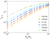 |
Fig. 1 Initial atmospheric mass fractions as a function of initial planetary masses for planets located at orbital separations of 0.03, 0.05, 0.1, 0.2, and 0.35 AU according to the basic setup (Eq. (1); purple to cyan lines) and to the migrated scenarios (green line) defined in the text. |
2.4 Stellar evolution models
The planetary atmospheric evolution models described in Sect. 2.1 require as input the stellar properties as a function of time as well to estimate the evolution of the atmospheric mass-loss rates and equilibrium temperature. In particular, the input should include the stellar bolometric luminosity (Lbol) and the XUV luminosity (Lxuv). Our framework employs the Mors stellar evolution code (Johnstone et al. 2021), which predicts the evolution of the stellar rotation period and translates it into Lxuv. In terms of stellar physics, the Mors code relies on the isochrones published by Spada et al. (2013).
As stars can be born with very different initial rotation rates (e.g., Tu et al. 2015), the rotation period, and thus Lxuv, can spread over more than an order of magnitude at young ages. In addition to comparing the relative input from initial atmospheric mass fractions and consequent atmospheric loss, one of the aims of this work is to study the extent to which this spread can affect the evolution of planetary atmospheres across a wide parameter range, and to determine whether this spread has a noticeable impact in the observed MR distribution. To model the evolution of the planetary atmospheres, we therefore employed three different evolutionary scenarios of the host star: that it evolved as a slow, as a medium, or as a fast rotator. As in Kubyshkina & Vidotto (2021), we considered for a solar mass star the evolutionary tracks corresponding to rotation periods of 1, 5, and 15 days at an age of 150 Myr for a solar mass star to account for the full possible spread.
Throughout, we considered just one possible host star of 1 M⊙, although the observed systems also comprise planets orbiting stars with a higher and lower mass than 1 M⊙. We limit this work to a host star with 1 M⊙ because the number of known exoplanets for which mass and radius are measured with sufficient accuracy is not large enough to enable splitting the sample into smaller subsets to account for different host star masses and still yield a meaningful comparison with model predictions. However, planetary atmospheric evolution depends to some extent on the mass of the host star. For example, Kubyshkina & Vidotto (2021) demonstrated that at the orbital separations corresponding to the same equilibrium temperatures around stars of different masses, planets orbiting 1 M⊙ stars preserve more of their primordial atmospheres than planets evolving around lower-mass stars. Moreover, because of the specifics of stellar evolution, the difference between fast and slowly rotating stars is more pronounced for higher-mass stars (e.g., Johnstone et al. 2021). Therefore, when observational uncertainties are accounted for, the comparison we present here remains adequate for planets orbiting stars with masses lying in the 0.8–1.2 M⊙ range (that of the majority of the observed systems considered in this work; Fig. 2), while for planets orbiting lower-mass stars, slight deviations from our model predictions toward smaller atmospheres (i.e. planetary radii) and a smaller spread in the MR distribution as a result of the rotation history of the host star are expected.
3 Observed mass-radius distribution of intermediate-mass planets
For the comparison with the modeling results, we extracted the sample of detected and confirmed planets from the NASA Exo-planet Archive2 employing the following filters. Because we did not restrict ourselves to Sun-like stars, we considered a range of orbital separations that is somewhat wider than that of the theoretical models by including planets with semi-major axes up to 0.4 AU. We further considered planets with masses in the 1–110 M⊕ range and required the planetary radius to be measured. Finally, we filtered the selected planets by considering just those with relative uncertainties on the planetary mass and radius smaller than 45 and 15%, respectively. The resulting data set comprises 199 planets. Figure 2 shows the data set distributions in terms of host star mass, equilibrium temperature, planetary mass, planetary radius, orbital period, and orbital semi-major axis.
Kubyshkina & Vidotto (2021) showed that when planets orbiting stars with different masses are compared, the equilibrium temperature rather than the orbital separation should be used for a comparison with models. To ensure consistency, we did not consider the equilibrium temperature indicated in the database, but computed it as
 (2)
(2)
where α is the planetary albedo, which we considered being equal to zero, a is the orbital separation, and Teff and R*, are the stellar effective temperature and radius extracted from the database. When Teff and/or R* were not available in the database, we extracted the missing information from Stassun et al. (2019).
Figure 2 indicates that most of the host stars in the considered data set have masses between 0.6 and 1.2 M⊙. The peak lies around 0.9 M⊙. The equilibrium temperatures of most of the planets range between 500 and 1500 K, which is comparable with the temperatures of the set of modeled planets, where Teq ranges from 512 K (a = 0.35 AU) to 1700 K (a = 0.03 AU). In terms of mass and radius, the set of considered planets is dominated by planets with masses below 20 M⊕ and radii smaller than 5 R⊕, which are expected to be significantly affected by atmospheric mass loss. Above these values, the mass distribution looks nearly uniform (except for a noticeable lack of planets with masses between 40 and 50 M⊕), while the radius distribution presents a secondary peak around 10 R⊕ (i.e., about the radius of Jupiter), which is mainly due to planets more massive than ~60 M⊕ and Teq around 1000 K. Driven by selection biases, most planets in the sample have short orbital periods, and thus short orbital separations.
For some of the planets (e.g., WASP-107 b and GJ 436 b), the NASA exoplanet archive provides more than one entry. In these cases, we computed the median value taking the largest error bar given by the single entries as uncertainty to finally obtain a single entry for each parameter.
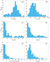 |
Fig. 2 (a) Distribution of host star mass, (b) equilibrium temperature, (c) planetary mass, (d) planetary radius, (e) orbital period, and (f) semimajor axis, for the considered data set of observed systems. |
4 Comparing model predictions with observations
4.1 Overall comparison
Before proceeding with the comparison, we summarize the properties of the database of theoretical models for clarity. The database consists of a set of individual atmospheric evolutionary tracks for planets starting their evolution with 20 different masses, at five different orbital separations, and around three 1 M⊙ stars, each with a different rotation history. In addition to these parameters, we considered two scenarios for the initial atmospheric mass fractions, where fat,0 increases with increasing planetary mass: the basic-setup scenario with more compact initial atmospheres (300 evolutionary tracks), and the migrated scenario, which assumes more voluminous initial atmospheres (100 evolutionary tracks assuming the host star evolves as a slow rotator, because we employed this scenario just to outline the upper boundary of the MR distribution).
All evolutionary tracks were run up to 10 Gyr. By combining all of them, we can therefore construct the theoretical MR distribution at any given moment in time between protoplanetary disk dispersal (5 Myr) and 10 Gyr. To compare the modeling results with the observations, we considered an age of 5 Gyr, which is about the average age of the observed planets. Although the age is poorly constrained for most systems, the MR distribution does not vary significantly at ages older than ~3 Gyr, and thus the particular choice of the comparison age does not modify the conclusions.
Figure 3 shows the comparison between the observed and synthetic MR distributions. We divided the 199 planets of the observed population into the six Teq intervals listed in Table 2. Therefore, we considered the smallest Rpl as a function of planetary mass obtained in our models at temperatures of 512 K (0.35 AU) and 680 K (0.2 AU) as the lower theoretical radius boundary (solid light blue line in Fig. 3) for planets with 512 K < Teq < 680 K. This lower boundary is given by synthetic planets with Teq = 680 K orbiting the fast-rotating star, because their initial atmospheres are smaller at 680 K than at 512 K (see Fig. 1) and mass loss is greater for closer-in planets and in the case of a fast rotator. Similarly, the upper radius boundary in this temperature range is set by the planets with lower Teq (i.e., 512 K) orbiting the slowly rotating star. We also considered two upper boundaries, the one predicted by the basic-setup scenario (short-dashed blue line in Fig. 3) and the one predicted by the migrated scenario (long-dashed light blue line in Fig. 3), where we considered the latter giving the predicted absolute maximum radius. We then applied the same scheme for all other temperature intervals (Table 2). The observed planets with Teq < 512 K and Teq > 1700 K lie outside of the boundaries of our synthetic population. We only give the lower and the upper radius limits for them.
The lines drawn in Fig. 3 also give the approximate location of the regions of the MR distribution controlled by atmospheric mass-loss or by atmospheric accretion or by a mix of the two for each temperature interval. The evolution is mostly controlled by atmospheric mass loss where the short-dashed (upper radius boundary within the basic-setup scenario) and long-dashed lines (upper radius boundary within the migrated scenario) overlap, meaning that the upper radius boundary is roughly independent of the initial atmospheric mass fraction. Instead, deviations between the short- and long-dashed lines indicate that atmospheric accretion plays a role in the evolution. Therefore, the distance of the short- to the long-dashed line with respect to the distance of the short-dashed to the solid line is proportional to the relative importance of atmospheric accretion over mass loss on the evolution for each planetary mass.
The spread in planetary radius obtained from the evolutionary tracks employing the basic-setup scenario resembles the observed MR distribution for planets up to 15–20 M⊕ well. This corresponds to the sub-Neptune mass planet population, whose evolution is thought to be mainly shaped by atmospheric escape. For these planets, the initial atmospheric mass fractions are not as important as what occurs for the more massive planets. This can be seen by comparing the light blue short-dashed and long-dashed light blue lines in Fig. 3, which show the final position of planets starting with very different initial conditions (basic-setup versus migrated scenario) and evolving at 0.35 AU (Teq = 512 K) around the slowly rotating star. These two lines converge at about 7 M⊕, reflecting the fact that below this mass, the differences of a factor of a few in the initial atmospheric mass fractions does not affect the final distribution. This effect was considered in detail by Kubyshkina et al. (2020). The convergence point between the two regimes shifts toward higher masses with decreasing orbital separation and reaches ~12 M⊕ at 0.03 AU (Teq = 1700 K, see Fig. A.2). Remarkably, the latter value is lower than the highest-mass bare core predicted in the basic-setup scenario (~20 M⊕). This means that at such a short orbital separation and at an age of a few billion years, planets with a present-day mass of 10–20 M⊕ can only host a hydrogen-dominated atmosphere if they started their evolution with a massive envelope. For example, the borderline case of a planet with a current mass of 12 M⊕ started its evolution as a 21.7 M⊕ planet comprising a 40% initial atmospheric mass fraction. After 5 Gyr, this planet has lost almost its entire primary atmosphere and still experiences significant mass loss, which would lead to complete atmospheric loss within an age of 6 Gyr.
For planets more massive than ~10 M⊕, the initial conditions therefore appear to be important for explaining the observed radius spread in the MR distribution, which requires higher initial atmospheric mass fractions than those estimated in the basic-setup scenario. When we consider the migrated scenario (where fat,0 varies from about 3% for a 1 M⊕ planet to 70% for a 108.6 M⊕ planet), the theoretical prediction fits most of the observed MR distribution well, except notably for the group of highly inflated hot planets with masses above ~60 M⊕ that we discuss in Sect. 4.3.
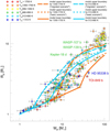 |
Fig. 3 MR distribution of the selected observed planets in comparison to modeling results. The symbol color indicates the approximate planetary equilibrium temperature as given in the legend. The largest uncertainties are 45% on planetary mass and 15% on planetary radius. The solid and long-dashed lines enclose the maximum predicted spreads in planetary radius at the age of 5 Gyr, obtained by considering the entire set of atmospheric evolutionary tracks computed in the 512–680 K (light blue lines) and 1350–1700 K (orange lines) temperature intervals, where the upper boundary is given by the migrated scenario. For reference, the short-dashed lines show the upper boundary predicted for the basicsetup scenario. |
Model boundaries for each considered Teq interval.
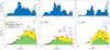 |
Fig. 4 The comparison between the observed ΔRpl,obs and synthetic ΔRpl,model radius spread values as a function of planetary mass for the whole temperature range and for planets cooler or hotter than 956 K. Bottom panels: Comparison between the measured (squares) and synthetic (areas) spread in planetary radii as a function of planetary mass (ΔRpl = Rpl,max – Rpl,min) for the entire sample (left), for planets cooler than 956 K (middle), and for planets hotter than 956 K (right). The relative values for the observed ΔRpl distribution are listed in Tables B.1–B.3, respectively, but with the difference that for visualisation purposes, we combined neighbouring bins whose ΔRpl values differed by less than 1% in the plots. In the high-mass range, the blue and black squares have been obtained by accounting and disregarding, respectively, planets affected by atmospheric inflation (i.e., planets with a radius larger than 11 R⊕). The green area is for the basic scenario and accounts for the variability in the initial stellar rotation rate affecting atmospheric mass loss. The yellow area is for the migrated scenario, and thus it accounts for larger initial atmospheric mass fractions (assuming the host star was a slow rotator). To guide the eye, the dashed red line is a smoothed distribution of the black squares. Top panels: Histograms of the number of observed planets within each mass bin for the entire sample (left), for planets cooler than 956 K (middle), and for planets hotter than 956 K (right). The dark blue and bright blue areas account for and disregard, respectively, planets affected by atmospheric inflation. |
4.2 Radius spread
To facilitate understanding the results described above, we present the comparison between the observed ΔRpl,obs and synthetic ΔRpl,model radius spread values as a function of planetary mass in Fig. 4. For the observed MR distribution (black squares in Fig. 4), we derived ΔRpl,obs as follows. We first divided the considered 1–110 M⊕ mass range into 50 bins equally distributed in logarithmic space and computed the running median mass of the planets falling into every 5 consecutive bins. We associated an uncertainty corresponding to the median error bar of the planets within each mass bin with each median mass value. For each mass bin, we then derived ΔRpl,obs by computing the difference between the radii of the largest  and smallest
  planets. We then derived the uncertainty on ΔRpl,obs (σΔRpl,obs) for each mass bin by computing the difference between ΔRpl,obs and the difference between the radius of the largest planet, plus the 1σ upper bound error bar
  , and the radius of the smallest planet, minus the 1σ lower bound error bar
  , that is, the sum of
  and
and 
![$\matrix{ {{\sigma _{\Delta {R_{{\rm{pl,obs}}}}}} = [(R_{{\rm{pl}},\max }^{{\rm{obs}}} + \sigma _{{R_{{\rm{pl,}}\max }}}^{{\rm{up}}}) - R_{{\rm{pl}},\min }^{{\rm{obs}}} - \sigma _{{R_{{\rm{pl,}}\min }}}^{{\rm{down}}}] - \Delta {R_{{\rm{pl,obs}}}}} \cr { = \sigma _{{R_{{\rm{pl,}}\max }}}^{{\rm{up}}} + \sigma _{{R_{{\rm{pl}},\min }}}^{{\rm{down}}}.} \cr } $](/articles/aa/full_html/2022/12/aa44916-22/aa44916-22-eq9.png) (3)
(3)
Table B.1 lists the ΔRpl values and their uncertainties obtained from the observed MR distribution for each mass bin, while Tables B.2 and B.3 give the ΔRpl values obtained considering planets with Teq lower and higher than 956 K, respectively.
Within the synthetic MR relation, ΔRpl odel is controlled by planets lying at different orbital separations, thus having different Teq values and receiving different amounts of stellar XUV flux throughout their evolution, implying that they experience different mass-loss rates. At each planetary mass, ΔRpl odel was therefore defined as the difference between the upper radius boundary at 512 K and the lower radius boundary at 1700 K (see Table 2) as follows:
 (4)
(4)
For any other temperature interval, we defined ΔRpl,model following Eq. (4) substituting  (512 K) and/or
  (1700 K) with those of the considered temperatures. In each interval, we considered
  obtained employing the basic-setup (green areas in the bottom panels of Fig. 4) and migrated scenario (yellow areas in bottom panels of Fig. 4).
By default, the ΔRpl,model values include the impact on planetary atmospheres of the different evolution of the stellar rotation rate, and thus of the different amounts of stellar XUV radiation emitted during the early evolutionary stages. The part of ΔRpl,model corresponding exclusively to the different possible evolution of the stellar rotation rate varies at different orbital separations and reaches its maximum value of ~1.1 R⊕ at the innermost orbit of 0.03 AU for planetary masses of ~26 M⊕. The maximum spread at other orbital separations, which is ~1.0 R⊕ at 0.1 AU and ~0.5 R⊕ at 0.35 AU, is achieved at lower masses, at ~11 M⊕ at 0.1 AU and at ~3 M⊕ at 0.35 AU. In all cases, these masses are close to the highest-mass bare cores predicted by our models, while the spread due to the differences in stellar histories decreases toward higher planetary masses due to the decreasing impact of escape. However, for the innermost orbit of 0.03 AU, this spread remains ~0.5 R⊕ around 80 M⊕. Thus, the total ΔRpl,model within the basic-setup scenario represents the sum of the spread due to the different stellar rotation histories with the spread caused by the different orbital separations, where the latter includes the effect of differences in irradiation levels and, where relevant (above ~10 M⊕), in initial atmospheric mass fractions. This total spread is shown by the green area in Fig. 4.
Both Figs. 3 and 4 show that ΔRpl is not uniform as a function of planetary mass. For the lowest-mass planets that have completely lost their atmospheres within 1 Gyr ΔRpl ≈ 0, it is highest for the intermediate-mass planets that keep some of their atmosphere even though they experience significant atmospheric escape, and moderate for the higher-mass planets that are only weakly affected by atmospheric escape (when planets with radii larger than 11 R⊕ are excluded, which are affected by atmospheric inflation; see Sect. 4.3). In terms of atmospheric escape mechanisms, the atmosphereless planets typically lose their atmospheres already within the first several hundred million years (e.g., Kubyshkina et al. 2018). For the intermediate-mass and massive planets, escape is mostly driven by the incident stellar XUV radiation, although for the latter group, atmospheric evolution is mostly driven by thermal contraction, rather than atmospheric escape.
Figure 4 shows that the ΔRpl,model predicted by the basic-setup scenario is a poor fit to the observed radius spread (at least for more massive planets). We therefore further considered the impact of possible planet migration by considering the migrated scenario (Sect. 2.3) on ΔRpl. Within the migrated scenario, the upper boundary of the radius spread is pushed upward (yellow area in Fig. 4), leading to a significantly better fit with the observations, particularly when we consider the entire sample and exclude the planets that are subject to atmospheric inflation. However, the quality of the fit decreases somewhat when the sample is split between low- (≤956 K) and high-temperature (>956K) planets.
In the low-temperature range, the synthetic ΔRpl distribution is a good fit to the observations up to about 12 M⊕, while it is underestimated at higher masses. This discrepancy is caused by a group of dense Neptune-mass planets (comprising about 12% of the observation data set) that lie outside of the model prediction, while the vast majority agrees with the models; we thoroughly disucss these outliers in Sect. 4.3.
In the high-temperature range, the models instead slightly underestimate the observed ΔRpl distribution up to about 9 M⊕ and slightly overestimate it at higher masses. Additional runs indicated that the reason of the mismatch at low mass might be that we considered a single stellar mass for the host star, while several planets in this temperature and mass range obit stars that are significantly more or less massive than 1 M⊙. This topic has been studied in detail by Kubyshkina & Vidotto (2021). Furthermore, our predictions for the lower-mass planets are sensitive to some of the model assumptions, such as core density, which alone can account for a radius spread of about 0.5 R⊕ (see, e.g., Fig. A.2), and age (see, e.g., Sect. 4.3). Instead, the mismatch at higher masses is no concern for the following reasons. First, the migrated scenario sets the absolute upper limit and is not intended to exactly fit the observed distribution. Second, the majority of planets with Teq > 956 K are concentrated near or above the upper boundaries predicted for the basic-setup scenario, suggesting that the majority of planets in this region would follow the migrated scenario. Because this lack of planets within the area predicted by the basic-setup scenario pushes the lower boundary of the observed population upward, we expect to see points within the yellow area. Finally, for planets more massive than 50 Me, the position of the observed distribution depends on where the boundary is set at which atmospheric inflation set in, which we set rather arbitrarily.
4.3 Outliers
In total, we find that about 20% of the 199 observed planets we considered lie outside of the boundaries drawn by the synthetic models. About half of them are hot and massive planets with radii above 10 Re (top right corner of Fig. 3). Except for a few exceptions, the remaining outliers are dense and relatively cool Neptune-mass planets, whose fraction increases with decreasing temperature: we find only 3 of them in 680–956 K interval (of 63 planets in total), but the number increases to 6 out of 28 planets in the 512–680 K interval and to 11 out of 22 for Teq < 512 K.
As shown by Figs. 3 and 4, the group of planets that diverges most strongly from the model predictions are sub-Saturns, with masses between 60 and 110 M⊕ and temperatures in the range of 800–1500 K. For these planets, the radii exceed 10–11 R⊕, and reach 12 R⊕ for Teq < 1000 K and 16.4 R⊕ for Teq between 1350 and 1500 K. Furthermore, the radii of these planets are clearly correlated with equilibrium temperature and planetary mass. Even within the migrated scenario and for 60–110 M⊕ planets (60–70% of the mass of these planets is in the atmosphere), such large radii are achieved only within the first 10 Myr of evolution, while planets are hot, but none of the observed planets in this group is younger than 1 Gyr. Although atmospheric mass loss is negligible for these planets (it reaches up to ~1012 g s−1 in the first billion years of evolution, but is unable to remove even 1% of the initial atmosphere), thermal contraction alone pushes the planetary radii below 10 R⊕ within a few tens of million years, independently of the assumed initial entropy (i.e., core temperature). We even attempted to reproduce the observed distribution by increasing the initial atmospheric mass fraction to 90%, but the resulting planetary radii hardly exceeded 10 R⊕.
This suggests that some additional heating mechanism (or cooling-suppression mechanism) is at play in inflating the radii of these planets. These objects might therefore represent the low-mass edge of the population of inflated hot Jupiters (Bodenheimer et al. 2001; Guillot & Showman 2002; Baraffe et al. 2003; Laughlin et al. 2011; Demory & Seager 2011; Fortney et al. 2021). However, Fig. 5 shows that for planets in this sample (Rpl > 10 R⊕ and Teq > 800 K), the dependence of radius on equilibrium temperature is about  , which is shallower than that found for hot Jupiters at temperatures above 1200 K, that is,
  (Laughlin et al. 2011). We remark that a more detailed analysis of the data indicates that the value of the exponent seems to depend on equilibrium temperature as well, but the still small size of the sample does not allow any robust conclusion. Furthermore, the group of inflated planets might extend down to ~500 K when planets with radii of 6–10 R⊕ and equilibrium temperatures below 1000 K (green points in Fig. 5) are also included. When these smaller, lower-temperature planets are included, the lowest planetary mass in the group of inflated sub-Saturns decreases from 38.1 M⊕ to 16.4 M⊕.
For context, a wide range of possible mechanisms has been put forward to explain the radius inflation of hot Jupiters. Due to the strong correlation with Teq (and stellar Teff), most theories suggest that atmospheric inflation is connected with star-planet interaction, which includes a number of specific processes that can be separated into three groups: tidal interactions with host star (e.g., Bodenheimer et al. 2001; Arras & Socrates 2010), hydrodynamic heat transport toward the planetary interior (e.g., Showman & Guillot 2002; Youdin & Mitchell 2010; Tremblin et al. 2017; Sainsbury-Martinez et al. 2019), and heating due to induced currents deep in the atmosphere (Ohmic dissipation or induction heating; Batygin & Stevenson 2010; Perna et al. 2010; Wu & Lithwick 2013; Ginzburg & Sari 2016; Kislyakova et al. 2018; Knierim et al. 2022).
In addition to the group of hot sub-Saturns, a few specific planets diverge from the modeling predictions and stand out compared to the other observed planets with comparable mass and temperature. Fig. 3 highlights the most evident outliers, which are WASP-107b, WASP-139b, Kepler-18d, TOI-849b, and HD 95338 b. The first three lie in the 680–956 K equilibrium temperature bin and their density is particularly low, while the latter two are located below the lower radius boundary for planets at an orbit equivalent to Teq = 700 K. Of these planets, WASP-139 b is the youngest, with an estimated age of ~0.5 Gyr (Hellier et al. 2017); the parameters of this planets agree with our predictions at the age of the system. WASP-139b should therefore not be considered to be an outlier. The same applies to the  Gyr old planet Kepler-9 c (see Fig. 6; Borsato et al. 2019) and possibly to π Men c as well (see Fig. A.3; Huang et al. 2018; Gandolfi et al. 2018).
TOI-849 b is consistent with the theoretical prediction given by the upper radius boundary shown in Fig. A.2. However, we highlight this planet because it is considerably more dense than planets of similar mass and temperature. Figures 3, A.2 and A.3 show that the majority of planets hotter than 1000 K lie near to or somewhat above the upper limit of the predicted radius spread within the basic-setup scenario (see the short-dashed red, orange, and yellow lines). This suggests that the relatively small initial atmospheres assumed in this scenario for hot planets are unlikely. To reproduce the MR distribution of planets hotter than 1500 K, the initial atmospheres should necessarily be substantial, as assumed in the migrated scenario (see the long-dashed red and orange lines in Fig. A.2), implying that these planets were formed farther away from the star and migrated inward, in agreement with recent formation theories (Morbidelli & Raymond 2016; Jin & Mordasini 2018; Morbidelli 2020). Instead, HD 95338 b has an equilibrium temperature of about 385 K (Díaz et al. 2020), and therefore lies far below the lower edge predicted for planets cooler than 512. Figure 6 shows that this is not an isolated case as there is a tendency for planets on the cold side (Teq < 680 K) of the distribution to behave in a similar way.
A significant fraction of the cooler planets (<680 K) lies below the lower boundaries predicted by the model (Fig. 6). Planets at these temperatures are less affected by atmospheric escape than the hotter planets, and their final position in the MR diagram is strongly dependent on their initial parameters. Therefore, we would expect to see such planets spread around the theoretical predictions because the initial mass fractions we employed are average values of those predicted by formations models. However, part of the outliers (especially for Teq < 512 K) stand out significantly, and their bulk density suggests that they can possess only small hydrogen-dominated atmospheres of less than 1–2%, which is an order of magnitude lower than the typical atmospheric mass fractions expected for planets in this part of the parameter space (e.g., HIP97166b, K2-292b, or K2-110b, GJ143b), but the possibility that the model underpredicts the mass-loss rates for these planets cannot be neglected.
Moreover, these planets may not match our prediction as a result of our assumption that all planets orbit a 1 M⊙ star. The observational data set is dominated by planets orbiting stars with masses below 0.7 M⊙ for planets cooler than 680 K and with masses below 0.5 M⊙ for planets cooler than 512 K, as indicated by the histograms in Fig. 6. Furthermore, the fraction of low-mass stars in the observational data set increases progressively with decreasing Teq (see also Figs. A.2–A.4), and the fraction of dense Neptunes lying below the boundaries predicted by our models behaves in the same way. The same temperatures are achieved at closer orbital separations for lower-mass stars, implying that at the same equilibrium temperature, planets orbiting lower-mass stars will lose more atmosphere than those orbiting higher-mass stars (e.g., Kubyshkina & Vidotto 2021). We also overestimated the results that might be obtained by applying Eq. (1) because the orbital separations take the specific stellar masses into account. To illustrate this, we used Eq. (1) to compute fat,0(a), that is, the initial atmospheric mass fraction obtained using the actual orbital separations (a) for the observed planets with Teq < 512 Κ and Mpl > 6 M⊕. We then again used Eq. (1) to compute fat,0(0.35 AU), that is, the initial atmospheric mass fraction obtained for the same planets, but assuming an orbital separation of 0.35 AU (i.e., the basic-setup scenario). Finally, we plot in Fig. 7 the ratio of fat,0(a) and fat,0(0.35 AU) as a function of the mass of the host stars. The ratio decreases with decreasing stellar mass, implying that to adequately model these planets, an atmospheric accretion model suitable for low-mass stars is required. However, a few outliers still fall in the category of dense Neptunes that orbit Sun-like stars (i.e., HD 95338 b, Kepler-411b, or K2-292b). Appendix A thoroughly discusses the single most important outliers from the theoretical MR distribution.
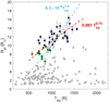 |
Fig. 5 Radii of the observed planets as a function of equilibrium temperature. The black points mark the group of inflated Saturns discussed in the text (Rpl ≥ 10 R⊕), and the green points are planets with 6 ≤ Rpl < 10 R⊕ and Teq < 1000 K. All other planets are marked in gray. The dashed red line shows the fit to the black points, and the dashed blue line shows the fit to these planets assuming the exponent obtained for the inflated hot Jupiters (Laughlin et al. 2011). |
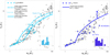 |
Fig. 6 Same as Fig. 3, but for the 512–680 Κ (left panel, light blue) and <512 Κ (right panel, dark blue) temperature range. Planets from other temperature intervals, shown in black, are included in the plots for clarity. The light blue (left panel) and dark blue (right panel) solid lines indicate the lower boundary of the theoretical radius spread for the respective temperature intervals. The long-dashed and short-dashed light blue lines (left panel) indicate the upper boundaries of the radius spread in the 512–680 Κ interval according to the migrated and basic-setup scenarios, respectively. For context, the inset located in the bottom right corner shows the mass distribution of the stars hosting the observed planets lying within each considered temperature range. |
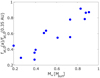 |
Fig. 7 Ratio of fat,0(a) and fat,0(0.35AU) as a function of host star mass for the observed planets with Teq < 512 Κ and Mpl > 6 M⊕. |
5 Escape-dominated and formation-dominated regions of the MR diagram
The analysis presented in Sect. 4.1 shows that combining average primordial planetary parameters predicted by formation models with atmospheric evolution describes the observed overall MR distribution well (see Figs. 3 and 4). Furthermore, our analysis highlights regions of the parameter space that are characterized by qualitatively different planetary origin and/or evolutionary path (Figs. 3 and 6).
Most of the radius spread for planets with a present-day mass below ~ 10 M⊕ is shaped by differences in atmospheric mass-loss rates caused by different orbital separations and different evolutionary tracks of the stellar rotation rate (see Fig. 4). For these planets, atmospheric loss is therefore the dominant mechanism driving atmospheric evolution. The primordial parameters characterizing these planets play a minor role in shaping the final MR distribution, as a wide range of possible initial parameters can lead to the same outcome (see Kubyshkina et al. 2018, 2019a, 2020).
Instead, atmospheric loss becomes progressively less relevant for more massive planets, and the atmospheric evolution of planets with masses higher than 60 M⊕ is mainly driven by thermal contraction. In this case, the initial planetary parameters play the leading role, in particular, the initial atmospheric mass fraction. To explain the upper part of the observed radius spread for planets more massive than 10 M⊕, we therefore have to assume that these planets were formed with large hydrogen-dominated envelopes (Fig. 3). This appears to be particularly important for planets in close-in orbits, where the radius spread corresponding to different initial conditions is up to four times broader than the maximum spread due to the different possible stellar evolutionary paths.
Finally, for orbits corresponding to Teq ≲ 700 K, the radius spread displayed by ~7–30 M⊕ planets is significantly broader than predicted by the models. A significant number of planets presents unexpectedly (for their temperature) high densities. This group of high-density planets comprises about 12% of the whole data set, suggesting that they represent a systematic deviation from the theoretical prediction, rather than individual outliers (see Fig. 6).
The atmospheric evolutionary models indicate that planets with Teq < 700 K and masses around 20–30 M⊕ are weakly affected by atmospheric escape (e.g., HD 95338 b), while the less massive planets can lose a substantial part of their atmosphere (e.g., K2-292b; see details in the appendix). However, for planets in the 7–30 M⊕ range, mass loss is not sufficient to entirely remove the primary hydrogen-dominated atmosphere, which is expected to be in the 7–40% range in the basic-setup scenario and to reach up to ~60% in the migrated scenario. These planets therefore had to start their evolution with atmospheric mass fractions similar to the present-day values (i.e., to have formed in a gas-poor environment) or to have lost their primary envelope as a result of some catastrophic event to reach radii comparable to those of the lower edge of the observed distribution. However, the second possibility is unlikely particularly because of the smooth deviation of the observed high-density planets from the rest of the population in the MR distribution (left panel of Fig. 6). This suggests that the underlying planetary structures, and thus the formation scenarios that led to them, in this temperature and mass range can be much more complex than that of a rocky core surrounded by a hydrogen-dominated envelope as considered in our models.
This shows that the relative role of the specific formation mechanisms and of atmospheric evolution driven by thermal contraction and mass loss in shaping the MR distribution of intermediate-mass planets is not the same in the entire parameter space. Figure 8 shows the impact of atmospheric escape (including the basic-setup and migrated scenario) at 50 Myr (near the end of the initial extreme mass-loss phase driven mainly by the own planetary thermal energy), 500 Myr (when the XUV emission of a moderate rotator decreases by an order of magnitude), and 5 Gyr in the different regions of the synthetic MR distribution (including all orbital separations considered in the model).
Already after 50 Myr of evolution, most planets with masses lower than 10 M⊕ lose more than 30% of their initial atmosphere. A significant fraction of planets finally has a bare core. This holds for planets within both scenarios (i.e., sets of initial parameters). Although the host star is most active at young ages, in the first 50 Myr and within the basic-setup scenario, the atmospheric escape endured by planets less massive than 10 M⊕ is mainly driven by their own thermal energy and low gravity (e.g., Kubyshkina et al. 2018; Kubyshkina & Vidotto 2021). In the migrated scenario, this is the case for planets less massive than ~20 M⊕ (see the top panel of Fig. 8). Since a significant fraction of their mass is in the atmosphere (~25–40% for the initial mass range of 9–20 M⊕) and these planets are highly vulnerable to escape (as a result of their large radii), these planets move significantly across the MR diagram toward lower masses and radii throughout their evolution.
Our models indicate that the initial phase of extreme escape forms the radius gap (e.g., Fulton et al. 2017; Owen & Wu 2017) around 1.8–2 M⊕ already after 50 Myr. Furthermore, Fig. 8 shows that the predicted position of the radius gap in the MR diagram is mass dependent, and it moves toward larger radii with increasing mass. In particular, at an age of 50 Myr, the radius gap extends up to 8 M⊕, and it extends to higher masses with time (about 15 M⊕ after 500 Myr and about 20 M⊕ at 5 Gyr) under the action of atmospheric escape driven by the stellar XUV irradiation. This demonstrates that (1) most of the atmospheric escape occurs within the first several tens to hundred million years, but (2) the long-term XUV driven escape on a timescale of a billion years plays a significant role in shaping the population of low-and intermediate-mass planets. At the end of the evolution, at 5 Gyr, the planets that have been significantly affected by atmospheric escape (i.e., lost at least 30% of their initial atmosphere) have masses as high as 60 Me, although the majority have masses below 20 M⊕.
Understanding the relative role of atmospheric escape and formation mechanisms with the consequent thermal evolution in shaping the MR relation is also important for the analysis of the evolution of planet-hosting stars. Kubyshkina et al. (2019a,b) and Bonfanti et al. (2021) developed an algorithm capable of constraining the past activity (rotation) history of stars hosting sub-Neptunes. The scheme is based on modeling the evolution of planetary atmospheres (similarly to the approach described in this study, but without thermal contraction) to constrain the initial planetary atmospheric mass fraction and evolution of the stellar rotation rate (a proxy for the stellar XUV emission) within a Markov chain Monte Carlo framework through fitting the present-day observed system parameters. One key prerequisite is that the radius of the planet should be sensitive to the activity history of the host star, which in turn requires that the planetary atmosphere is significantly affected by mass loss. However, there is no linear relation between differences in the lost atmospheric mass and differences in planetary radii between planets evolving around stars with different activity histories. The final differences in planetary radii additionally depend on mass and orbital separation of the planet (Kubyshkina & Vidotto 2021). Figure 9 shows how the relative difference in planetary radii caused by different rotation scenarios of the host star changes across the synthetic population within the basic-setup scenario. Here,
 (5)
(5)
where Rpl,slow/medium/fast are the final (5 Gyr) radii of the same planet orbiting around a slow, medium, or fast rotator. The maximum AR in our synthetic population is about 43% and exceeds 10% for a significant part of the population. For this to enable constraining the history of the activity of the host star, AR should be larger than the measured uncertainty on the planetary radius. For comparison, the relative uncertainty on the planetary radius for 96% of the detected planets considered in this work is smaller than 30%.
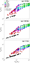 |
Fig. 8 Synthetic MR diagram color-coded according to the fraction of primordial atmosphere that has been lost through escape at 50 Myr (top), 500 Myr (middle), and 5 Gyr (bottom) for the entire model population (i.e., 0.03–0.35 AU). The color code is defined in the legend in the top left corner of the top panel. Circles and diamonds correspond to the initial conditions set according to the basic-setup and migrated scenarios, respectively. |
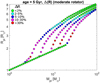 |
Fig. 9 Synthetic MR diagram color-coded according to the relative difference in planetary radii between planets that evolved around a slow, medium, and fast rotator at an age of 5 Gyr (see Eq. (5)), as indicated in the legend. The position of the points shown in Fig. 9 is that obtained for the basic-setup scenario considering a moderate rotator following interpolation on a regular mass grid. |
6 Conclusions
We have analyzed the MR distribution of low- and intermediate-mass planets by comparing it to the predictions of theoretical models computed by joining MESA with the results of upper atmosphere hydrodynamic simulations to accurately estimate mass-loss rates. This grid of hydrodynamic models covers planets in the 1–110 M⊕ mass range and 300–2000 K temperature range, which set up the applicability boundaries of our evolution models. To ensure that the comparison with the observed MR distribution is not significantly affected by observational uncertainties, we considered only planets with uncertainties smaller than 15% in radius and 45% in mass, which left a sample of 199 planets. Most of these planets orbit Sun-like stars, and we therefore considered all synthetic planets orbiting a 1 M⊙ star, but accounted for different scenarios of stellar activity evolution. In terms of initial atmospheric mass fractions, we used predictions derived from detailed formation models as a function of planetary masses and orbital separations (basic-setup scenario) or assuming formation at 1.5 AU and follow-up migration inside the disk (migrated scenario).
Studying the population of detected exoplanets is key to constrain fundamental planetary formation and evolution processes (e.g., atmospheric accretion and escape, migration, or core composition). So far, studies of the exoplanet population focused mostly on the planetary orbital period versus radius diagram, with the occasional addition of the stellar mass as a further parameter. Here, we demonstrated that based on ongoing ground- and space-based surveys, the currently available exoplanet population enables us to also consider the planetary mass, which is a key parameter controlling several physical processes, such as atmospheric accretion, atmospheric escape, and migration.
The observed MR distribution is shaped by a combination of planetary formation processes that determine the properties of planetary systems during the first several million years of evolution, and long-term atmospheric evolution driven by thermal contraction (slow dissipation of post-formation luminosity) and mass loss. Our evolution models reproduce the shape of the observed MR distribution well, even though we used a coarse approximation to estimate the initial atmospheric mass fractions. Furthermore, we showed that the relative impact on the shape of the MR distribution given by the initial planetary parameters and the consequent evolution is varies across the observed population. The boundary between escape-dominated and formationdominated regions of the MR distribution has a complex shape and cannot be attributed to one specific parameter, such as planetary mass or orbital separation.
In general, the low-mass part (Mpl ≤ 10 M⊕) of the population is fully dominated by atmospheric loss. All planets in this mass range are subject to extreme atmospheric escape driven by their own high thermal energy and low gravity throughout the first few tens of megayears of their evolution. This atmospheric loss becomes more intense with increasing planetary radius, and thus with increasing planetary core temperature and atmospheric mass fraction. Our simulations predict that increasing any of these two parameters at the time of the protoplanetary disk dispersal does not lead to significant changes in the final planetary properties after some billion years of evolution (see, e.g., Kubyshkina et al. 2019a; Kubyshkina & Vidotto 2021, for a detailed discussion). Recovering the initial parameters of these planets from their present-day properties is therefore difficult in general.
For more massive planets (Μpl ≥ 10 M⊕), the initial atmospheric conditions and the specific formation processes that led to them become important. In particular, we had to assume that planets formed with substantial hydrogen-dominated atmospheres (potentially beyond the snow line) to explain the upper part of the MR distribution. In this part of the distribution, the maximum radius spread associated with atmospheric mass loss, including the impact of the different paths of stellar rotation evolution, is about one-fourth of the entire spread. Furthermore, the relative contribution of the initial conditions on atmospheric evolution and thus on the radius spread depends on the orbital separation (i.e., equilibrium temperature). For planets cooler than Teq ~ 700 K, escape plays a significant role in atmospheric evolution up to 20–30 M⊕. At Teq ~ 1000 K, this mass boundary lies around 40–50 M⊕, and for the hottest planets, it moves up to 100 M⊕. However, the impact of the initial conditions remains dominant in all cases, particularly for the hottest planets.
The atmospheric evolution models we presented explain the position of about 80% of the detected planets with well-measured masses and radii in the MR diagram. The remaining 20% is mostly distributed into two distinct groups of outliers. The first group consists of about 8.5% of the total number of planets and comprises inflated sub-Saturns in close orbits (2–6 days) around their host stars, which require some kind of additional internal heat source to reproduce their radii, which are larger than predicted by the model. The strong correlation between radius and equilibrium temperature displayed by these planets indicates that the additional heating mechanism is probably similar, if not the same, as the mechanism that inflates the radii of hot Jupiters. The detailed analysis of WASP-107b suggests that this additional heating mechanism can also be effective for relatively cool (~700 K) and low-mass (~30–40 M⊕) planets.
The second group of outliers consists of about 12% of the total number of planets and comprises dense sub-Neptune-size planets with Teq ≤ 700 K and masses between 10 and 30 M⊕ in general. The simulations indicate that to achieve the observed planetary parameters at ages of a few billion years, the most extreme of these planets had to be formed with atmospheric mass fractions comparable to those currently present, namely ~ 1–2%, which is an order of magnitude smaller than predicted by the atmospheric accretion models used in this study. At the same time, the mass-radius relation of these planets resembles that of icy cores (Zeng et al. 2021), which might suggest that their internal structure is different from that of a rocky core surrounded by a hydrogen-dominated envelope, thus providing an alternative explanation. Independently of the core composition (e.g., icy or rocky with a large water fraction), the question of why these planets begin their evolution with a small primary envelope remains unanswered.
We showed that a crude parametrization of the results of planet formation models in combination with detailed atmospheric evolution models driven by thermal contraction and mass loss already fits the observed MR distribution well. Our analysis also demonstrated that this distribution cannot be shaped by one specific process, such as atmospheric accretion or escape, but is guided instead by a combination of a wide range of processes, including formation of planetary systems, planetary migration, and interactions between close-in planets and their host stars. To improve our understanding of the observed planetary distribution, these processes therefore have to be considered simultaneously in order to use the MR distribution as a diagnostic of planet formation (e.g., Venturini et al. 2020).
Acknowledgements
This research has made use of the NASA Exoplanet Archive, which is operated by the California Institute of Technology, under contract with the National Aeronautics and Space Administration under the Exoplanet Exploration Program.
Appendix A Systems deviating from the predicted MR distribution
We thoroughly discuss below the case of TOI-849 b. For the other planets, we mainly confirm whether they are real outliers or if their conflicting position in the MR diagram is the result of specific system parameters, such as a significantly different stellar host mass from the 1 M⊙ considered in this work. All planets discussed in this section are highlighted in Figure A.1. Figures A.2–A.4 are analogous to Figure 6, but show the hotter temperature intervals, namely Teq > 1350 K, 956–1359 K, and 680–956 K.
Appendix A.1 TOI-849b
TOI-849 b is an outlier compared not only to the modeling predictions, but also (and to a greater extent) to the rest of the observed population. Armstrong et al. (2020) reported a planetary radius of  and mass of
  , which correspond to an Earth-like density of
  . Therefore, TOI-849b appears to be a ≈3.5 R⊕ bare core, for which internal structure modeling concluded that the hydrogen-helium fraction does not exceed
  of the total planetary mass (Armstrong et al. 2020). This is similar to the model planets of similar mass and orbital separation within our basic setup when assuming the fast-rotating host star, which have a hydrogen-helium fraction of 2–3% at the age of TOI-849b (~7 Gyr).
Pezzotti et al. (2021) studied the possible migration history of TOI-849 b as a result of stellar dynamical tides in detail, assuming different initial planetary orbits and masses. They concluded that the planet could lie in its current orbit only if it was there already at the time of protoplanetary disk dispersal and the host star evolved as a slow or moderate rotator (the initial stellar rotation rate did not exceed 5 × Ω⊙, which is nearly equivalent to the moderate rotator case considered in this work). They also found that in this scenario, the atmosphere of TOI-849 b fully escaped within 30 Myr independently of the initial atmospheric mass fraction and planetary mass, which is not consistent with our results as described below, however.
In our basic-setup scenario, the initial atmospheric mass fraction of TOI-849 b would be 15%. However, as mentioned in Section 2.3, a gas-poor formation scenario such as this for a planet at this close orbital separation is rather unlikely, which is confirmed by the absence of compact massive planets at 0.03 AU (see the solid and short-dashed lines in Figure 3). To verify this scenario considering the actual planetary parameters, we ran atmospheric evolution assuming that the star evolved as a moderate rotator and employing a stellar mass of 0.929 M⊙, an initial atmospheric mass fraction of 15%, and an initial planetary mass of 46 M⊕. In this case, the model predicts total atmospheric loss within 1.9 Gyr, with a final planetary radius equal to the core radius (~ 2.7 R⊕), which is considerably smaller than the observed one ( ), however. The same is also true for the case of a slowly rotating star, although the lifetime of the atmosphere extends to almost 5 Gyr. Even though TOI-849 b is located near the lower boundary predicted for planets with comparable temperature, the assumed basic-setup scenario with a compact initial envelope therefore does not appear to be realistic for this specific planet.
We also tested a concurrent evolutionary path, namely that of an evaporated gas giant, by assuming that TOI-849 b started its evolution with a more massive hydrogen-dominated atmosphere. This scenario is realistic because at the orbit of TOI-849 b, higher-mass planets can also be subject to strong atmospheric escape. The mass-loss rates in the early stages of evolution might even be higher than those of planets with more compact envelopes (Kubyshkina & Vidotto 2021). Therefore, we ran a few additional models with fat,0 = 20 − 60% and consequently higher initial masses, always assuming that the present-day mass of TOI-849 b is nearly equal to that of the core. Starting from this setup, we ran the atmospheric evolution considering slowly, moderately, and fast-rotating host stars.
In the case of the slow rotator, the measured parameters of TOI-849 b can be reproduced with an initial atmospheric mass fraction of ~ 30 − 40%, corresponding to Mpl,0 ~ 51.8 − 55.8 M⊕. At the lower boundary of this interval, the entire atmosphere is lost within 9 Gyr, which is younger than the age given by the upper limit inferred for TOI-849. In the case of the moderate rotator, the required initial atmospheric mass increases to fat,0~ 50 – 60% (Mpl,0 ~ 76.6 – 95 M⊕). Finally, we find that for the fast-rotating star, the planetary atmosphere is lost in a time shorter than the age of TOI-849 b (accounting for the uncertainties) for all considered fat,0 up to 60%, leaving behind the bare core with a radius that is at least 0.5 R⊕smaller than the observed one; for higher initial atmospheric mass fractions, the atmosphere becomes unstable because the planetary radius at the time of the disk dispersal is too large.
The atmospheric escape, and hence the evolution of TOI-849 b, depends strongly on the evolution of its host star. The initial atmospheric mass fraction of 50% and initial mass of 76.6 M⊕ allow reproducing the planet in the case of the moderate rotator (radius of 3.35-3.86 R⊕ at  Gyr). A planet with the same initial properties, but evolving around a fast rotator would lose its atmosphere within 5 Gyr, and the maximum radius of the planet within the estimated age uncertainty reaches only ~2.9 R⊕. Instead, considering a slowly rotating star, the same planet finally has a radius of 4.0–4.6 R⊕ within 4.3–9.6 Gyr. At the orbit of TOI-849 b, even a planet born more massive than 70 M⊕ therefore experiences intense atmospheric escape throughout its entire life, and the final properties are strongly bound to the rotation history of the host star.
To summarize, TOI-849 b started its evolution most likely as a hot Saturn with a mass of ~ 50 – 85 M⊕, while the host star has evolved as a slow or moderate rotator. In the case of a moderate rotator, the initial mass of the planet (and corresponding initial atmospheric mass fraction) was close to the limit for which the atmosphere of the young planet is unstable to escape. Furthermore, because the computed atmospheric mass-loss rates are high throughout the entire evolution (up to about 5 × 10¹⁰ g s−1 at the current age of the system), it is possible that the planet is at the verge of losing its entire atmosphere.
As mentioned above, these results are somewhat different from those presented by Pezzotti et al. (2021). Although both studies considered similar initial planetary masses and concluded with the full escape of the atmosphere, the timescales predicted for this to occur are significantly different: on the order of billion years compared to the about 30 Myr obtained by Pezzotti et al. (2021). Furthermore, in the frame of our models, it is possible to reproduce the present-day parameters of TOI-849 b by employing higher initial masses and atmospheric mass fractions (30-40% in the case of the slow rotator and 50–60% for the moderate rotator) because the disruption of the atmosphere due to overinflation occurs at about twice the mass (~90 M⊕ against 46 M⊕). This is probably due to differences in the modeling approach. The three key components of the atmospheric evolution models (planetary structure models relating atmospheric mass fraction and basic parameters, stellar evolution models, and atmospheric escape model) differ between the two works, and although the physics underneath the models is qualitatively similar, the differences lead to evident divergences in extreme cases, such as that of TOI-849b.
Appendix A.2 HD110113b
HD110113 b is a hot mini-Neptune located within the radius valley. It is expected to host a hydrogen-dominated atmosphere of 0.1–1% (Osborn et al. 2021). In the MR diagram, the planetary properties (4.55 ± 0.62 M⊕; 2.05 ± 0.12 R⊕) place it near the upper limit predicted for planets with an equilibrium temperature of ≈600 K, that is, half that of the planet of ~1370 K (Osborn et al. 2021). The neighboring planet in the mass-radius diagram in the same temperature bin, π Men c (Huang et al. 2018; Gandolfi et al. 2018), has very similar parameters, but lower Teq, therefore we focused on the more extreme planet, that is, HD110113 b.
We probed the evolution of the planetary atmosphere assuming initial atmospheric mass fractions ranging between 1.5% and 70% (in the latter case, the mass of the atmosphere is ~5.7 times that of the core, and an even larger atmospheric mass fraction would lead to an unstable atmosphere), finding that at the position of HD110113b, the whole atmosphere escapes within 16 Myr–1.1 Gyr. Therefore, according to our models, HD110113 b should not possess any hydrogen-dominated atmosphere, which makes it an actual outlier with respect to the modeling results.
The small size of the planet makes the core composition an important factor for interpreting the observed planetary radius. Because of the planetary mass, the rocky core should have a radius of 1.45–1.56 R⊕, which requires some atmosphere to explain the observed radius. We note, however, that the measured planetary parameters are also consistent with a bare icy core (Zeng et al. 2021).
An alternative possibility for explaining the radius of HD110113b would be the presence of a secondary atmosphere, which might contain high-altitude hazes leading to a significant radius enhancement (Lammer et al. 2016; Gao & Zhang 2020), which is different to the case of hydrogen-dominated atmospheres considered by our models.
Appendix A.3 WASP-107b
WASP-107b is about twice the mass of Neptune and has a Jupiter-like radius (Dai & Winn 2017; Močnik et al. 2017; Piaulet et al. 2021), which stands out because of its low density. All radii published for WASP-107b significantly exceed the radii of planets a with similar mass and temperature, as well as the maximum radius predicted by our theoretical models. When the dependence of Rpl on equilibrium temperature (Figure 5) is considered, WASP-107 b lies at the lower Teq boundary of this group of planets. This suggests that despite the relatively low Teq of 736 ± 17 K, atmospheric inflation might also be at work on this planet.
To confirm that WASP-107 b is an outlier with respect to our theoretical model and belongs to the inflated planets, we ran a few additional evolutionary models assuming different fat,0, the measured system parameters, and a slowly rotating host star (to decrease mass loss). In this way, we determined the largest possible predicted planetary radius. Assuming an initial atmospheric mass fraction consistent with our basic-setup scenario of ~ 30%, we obtained a radius of 5.2–5.5 R⊕, which is about half the measured radius and even smaller than the estimate we obtained considering a solar-mass star (in agreement with Kubyshkina & Vidotto 2021).
For larger initial atmospheric mass fractions, mass loss throughout the evolution is relatively low and does not exceed ~12% of the initial planetary mass. However, at the estimated age of the system, the radius of the planet predicted by our models reaches a maximum value of 8.4 R⊕ for an initial atmospheric mass fraction of 65%. For larger initial atmospheric mass fractions, the atmosphere of the young planet becomes unstable even for a very low initial entropy (temperature) of the planetary core. For the coldest core and fat,0, the photospheric radius at an age of 5 Myr exceeds ~40 times the planetary Roche radius, which leads to fast atmospheric disruption.
We made the above estimates assuming a slowly rotating star (Prot,150Myr = 15 days) to derive an upper limit for the planetary radius. However, the rotation period of the host star of 17.5 ± 1.4 days is atypically short for the stellar age of 8.30 ± 4.30 Gyr (Močnik et al. 2017). According to the Mors models, this rotation period is compatible with an age of ~ 0.5 – 1.3 Gyr, depending on the specific rotation evolution of the star. The age estimates reported by Močnik et al. (8.3 ± 4.3 Gyr 2017) and Piaulet et al. (3.4 ± 0.7 Gyr 2021) are based on the comparison of the stellar parameters with isochrones, which can be considerably model dependent. However, even if the system is as young as 0.5 Gyr, the maximum radius reached within our test models (excluding unstable atmospheres) is 9.7 R⊕, which is considerably smaller than the measured planetary radius. In the light of these results, we conclude that the large radius of WASP-107 b is most likely the result of atmospheric inflation, which cannot be reproduced within the frame of our models.
In this respect, the atypically fast rotation of the host star might give an indication about the atmospheric inflation mechanism. The impact of both tidal and induction heating is expected to increase with increasing rotation rate of the host star (in the case of induction heating, the fast rotation implies a stronger magnetic field). Due to the orbital inclination of almost 90° (Močnik et al. 2017) and small orbital separation, induction heating might be particularly effective (Kislyakova et al. 2018). Instead, tidal heating requires an eccentric orbit, which is not the case for WASP-107 b. Furthermore, the low mass and relatively low temperature of WASP-107 b mean that both vertical heat transport and Ohmic dissipation (the latter requiring a high planetary magnetic field) are unlikely to be effective. This makes induction heating a possible inflation mechanism in this particular case. However, a separate and detailed study is necessary to draw any firmer conclusion.
Appendix A.4 Kepler-18d
Kepler-18d is a member of a relatively old (10.0 ± 2.3 Gyr) planetary system comprising two outer low-density Neptune-mass planets and an inner super-Earth orbiting a solar-mass star (Cochran et al. 2011; Hadden & Lithwick 2014; Morton et al. 2016; Berger et al. 2018). Planets c and d can be classified as super-puffs, and the relatively large mass uncertainty of the inner planet does not rule out the possibility of it hosting a thin hydrogen-dominated atmosphere. The large radius of 6.98 ± 0.33 R⊕ of Kepler-18 d is about one Earth radius above the upper boundary predicted by our theoretical models (see Figure 3 and 6). However, these considerations are based on the default parameters listed in the NASA Exoplanet Archive based on Cochran et al. (2011), but later measurements suggest smaller planetary radii of  (Hadden & Lith-wick 2014),
  (Morton et al. 2016), and
  (Berger et al. 2018), and also slightly lower planetary masses. These more recent values then place Kepler-18 d at the upper edge of our synthetic population. Despite this, we decided to consider Kepler-18 d in more detail, as it orbits a solar-mass star. This is at odds with its location near the upper boundary. To this end, we ran additional evolutionary models assuming different initial atmospheric mass fractions.
As expected, the models considering an initial atmospheric mass fraction of 12%, compatible with the basic-setup scenario, lead to a too-small radius of ~ 3.2 R⊕. To reproduce the present-day planetary parameters published by Cochran et al. (2011) and assuming a slowly rotating star, an initial atmospheric mass fraction of ~60% must be assumed, which is about 1.5 times higher than the fraction assumed for the planetary mass range in the migrated scenario. The smaller radii given by the other studies lead to initial mass fractions of about 40%, which fits our predictions well.
Similarly to the case of WASP-107b, the rotation period of the host star of about 12 days (Cochran et al. 2011) is atypically short for its age of 10.0 ± 2.3 Gyr. The Mors model predicts a gyrochronological age of about 1–2 Gyr. At this age, the planetary radius published by Cochran et al. (2011) would be compatible with that predicted considering an initial atmospheric mass fraction of 40%. To summarize, a detailed analysis shows that Kepler-18 d should not be considered as a real outlier because its position in the MR diagram relative to the models can be explained by slightly different initial conditions and/or a possible uncertainty on the age (and eventually radius) determination.
Appendix A.5 HD95338b
HD95338 b (Díaz et al. 2020) lies below the lower boundary of the total radius spread predicted by the models. The planet mass is about twice as high as that of Neptune, orbits relatively far from its host star (Teq ≃ 385 K), and has a radius of  , which is smaller than the smallest radii predicted for very close-in planets with Teq ~ 1700 K. To reproduce the observations, Díaz et al. (2020) suggested that the atmosphere of HD95338 b might be composed of a mixture of ammonia, water, and methane with a heavy-element enrichment of about 90%. For comparison, we considered a planet with parameters similar to those of HD95338 b, starting its evolution with ~ 40% of its mass contained in a hydrogen-dominated atmosphere. The evolution models suggest that such a planet would preserve most of the initial envelope until its current age.
We performed atmospheric evolution simulations assuming two different sets of initial parameters: (1) the planet started its evolution with an initial atmospheric mass fraction of 60% (and consequently higher mass), and (2) the planet started with parameters comparable to the present-day ones with a median mass of 42.4 M⊕ and initial atmospheric mass fractions of 10%, 7%, and 5%. For the host star, we considered a mass of 0.83 M⊙ and a rotation evolution equivalent to the cases of moderate and fast rotators considered in our study, but for the specific stellar mass.
In all cases, the atmospheric mass loss (induced mainly by stellar irradiation) does not affect much the evolution of the planetary atmosphere (radius), which decreases just by less than 0.1% of the planetary mass. Therefore, a planet that starts with a voluminous atmosphere reaches the age of HD95338 b (about 5 Gyr) with a radius nearly twice larger than the observed one. The three models starting with initial atmospheric mass fractions of 10%, 7%, and 5% lead to radii of 4.3–1.4 R⊕, 4.01–1.07 R⊕, and 3.75–3.8 R⊕, respectively. The last two values fall into the uncertainty radius range measured for HD95338 b, and the mass of the atmosphere remains nearly unchanged throughout the evolution in all three cases. Therefore, our models suggest that either this planet was formed with an initial atmospheric mass fraction similar to that observed now, or it lost its primordial hydrogen-dominated atmosphere, assuming it had one, possibly as a result of a catastrophic event.
Appendix A.6 K2-292b
K2-292b is a warm sub-Neptune orbiting at 0.13 AU around a solar-like star (Luque et al. 2019). Similarly to the case of HD95338 b, the planet lies below the lower boundary of the total radius spread predicted by the models. The planetary mass of 24.5 ± 4.0 R⊕ and radius of  result in a bulk density of
  , suggesting that the planet is most likely rocky and might host a secondary atmosphere. However, according to our simulations, if the planet were to start with a substantial primordial envelope of fat,0 ~10–30%, which is likely for its mass, it would preserve more than about 60% of it.
To confirm that the small radius of K2-292b is not a consequence of the specific system configuration, we ran a few additional evolutionary models assuming the present-day orbital parameters of K2-292b, a fast-rotating star (to favor mass loss to obtain the minimum possible radius), and a range of different initial atmospheric mass fractions between 1% and 70%. For all computed tracks, we find that the total atmospheric mass loss does not exceed ~ 6.2% of the planetary mass, and the present-day radius of the planet can only be reproduced assuming an initial atmospheric mass fraction of 1–2%.
Appendix A.7 GJ143b
GJ143b (aka HD21749b) is a dense warm (~ 422 K) sub-Neptune orbiting a K-type main-sequence star of 0.73 ± 0.07 M⊕. The planetary mass of  and radius of
  lead to a bulk density of
  , which is compatible with a purely rocky composition (Dragomir et al. 2019). However, when it starts with a substantial envelope of 25–30% as for our basic-setup scenario, a planet like this would preserve most of its atmosphere and currently have a radius of ~6 R⊕. Because the host star is considerably lighter than the solar-mass star considered by our model, we expect that GJ 143 b experienced higher atmospheric loss and finally reached a smaller radius than predicted. However, at the planetary orbit of 0.1915 AU, corresponding to an equilibrium temperature of ~ 422 K, these differences are not expected to be dramatic (Kubyshkina & Vidotto 2021).
To quantify the difference and to identify the possible initial parameters of GJ 143 b, we ran atmospheric evolutionary models assuming initial atmospheric mass fractions in the range 1–30%. We excluded larger initial atmospheric mass fractions, as the case of GJ 143 b is very similar to that of K2-292 b, except for the cooler temperature of GJ 143 b, and thus even lower expected atmospheric escape. Assuming an initial atmospheric mass fraction of 30%, compatible with the basic-setup scenario, we arrive at a current radius larger than ~ 5.35 R⊕. This is only slightly smaller than the predicted radius, which was obtained considering a solar mass star. This confirms that this is an outlier with respect to our modeling results. To reproduce the observed planet parameters in the frame of our evolutionary models, the initial atmospheric mass fraction should not exceed ~ 1%.
Appendix B Radius spread of the observed exoplanet distribution
Here we present the observational radius spread discussed in Section 4.1. The data underlying Figure 4 without optimization of the intervals are listed in Tables B (all temperatures), B (Teq ≤ 1000 K), and B (Teq > 1000 K).
Radius spread against planetary mass observed for planets with Teq in 512–1700 K range.
Radius spread against planetary mass observed for planets with Teq ≤ 956 K.
Radius spread against planetary mass observed for planets with Teq > 956 K.
References
- Armstrong, D. J., Lopez, T. A., Adibekyan, V., et al. 2020, Nature, 583, 39 [Google Scholar]
- Arras, P., & Socrates, A. 2010, ApJ, 714, 1 [Google Scholar]
- Baraffe, I., Chabrier, G., Barman, T. S., Allard, F., & Hauschildt, P. H. 2003, A&A, 402, 701 [NASA ADS] [CrossRef] [EDP Sciences] [Google Scholar]
- Batygin, K., & Stevenson, D. J. 2010, ApJ, 714, L238 [NASA ADS] [CrossRef] [Google Scholar]
- Bell, K. R., & Lin, D. N. C. 1994, ApJ, 427, 987 [NASA ADS] [CrossRef] [Google Scholar]
- Berger, T. A., Huber, D., Gaidos, E., & van Saders, J. L. 2018, ApJ, 866, 99 [NASA ADS] [CrossRef] [Google Scholar]
- Bodenheimer, P., Lin, D. N. C., & Mardling, R. A. 2001, ApJ, 548, 466 [NASA ADS] [CrossRef] [Google Scholar]
- Bonfanti, A., Fossati, L., Kubyshkina, D., & Cubillos, P. E. 2021, A&A, 656, A157 [NASA ADS] [CrossRef] [EDP Sciences] [Google Scholar]
- Borsato, L., Malavolta, L., Piotto, G., et al. 2019, MNRAS, 484, 3233 [NASA ADS] [CrossRef] [Google Scholar]
- Chen, H., & Rogers, L. A. 2016, ApJ, 831, 180 [Google Scholar]
- Cochran, W. D., Fabrycky, D. C., Torres, G., et al. 2011, ApJS, 197, 7 [NASA ADS] [CrossRef] [Google Scholar]
- Dai, F., & Winn, J. N. 2017, AJ, 153, 205 [NASA ADS] [CrossRef] [Google Scholar]
- David, T. J., Contardo, G., Sandoval, A., et al. 2021, AJ, 161, 265 [NASA ADS] [CrossRef] [Google Scholar]
- Demory, B.-O., & Seager, S. 2011, ApJS, 197, 12 [NASA ADS] [CrossRef] [Google Scholar]
- Díaz, M. R., Jenkins, J. S., Feng, F., et al. 2020, MNRAS, 496, 4330 [CrossRef] [Google Scholar]
- Dorn, C., Venturini, J., Khan, A., et al. 2017, A&A, 597, A37 [NASA ADS] [CrossRef] [EDP Sciences] [Google Scholar]
- Dragomir, D., Teske, J., Günther, M. N., et al. 2019, ApJ, 875, L7 [Google Scholar]
- Fortney, J. J., Dawson, R. I., & Komacek, T. D. 2021, J. Geophys. Res. Planets, 126, e06629 [NASA ADS] [CrossRef] [Google Scholar]
- Freedman, R. S., Lustig-Yaeger, J., Fortney, J. J., et al. 2014, ApJS, 214, 25 [CrossRef] [Google Scholar]
- Fulton, B. J., & Petigura, E. A. 2018, AJ, 156, 264 [Google Scholar]
- Fulton, B. J., Petigura, E. A., Howard, A. W., et al. 2017, AJ, 154, 109 [Google Scholar]
- Gandolfi, D., Barragán, O., Livingston, J. H., et al. 2018, A&A, 619, L10 [NASA ADS] [CrossRef] [EDP Sciences] [Google Scholar]
- Gao, P., & Zhang, X. 2020, ApJ, 890, 93 [Google Scholar]
- Ginzburg, S., & Sari, R. 2016, ApJ, 819, 116 [NASA ADS] [CrossRef] [Google Scholar]
- Ginzburg, S., Schlichting, H. E., & Sari, R. 2018, MNRAS, 476, 759 [Google Scholar]
- Guillot, T., & Showman, A. P. 2002, A&A, 385, 156 [NASA ADS] [CrossRef] [EDP Sciences] [Google Scholar]
- Gupta, A., & Schlichting, H. E. 2019, MNRAS, 487, 24 [Google Scholar]
- Hadden, S., & Lithwick, Y. 2014, ApJ, 787, 80 [Google Scholar]
- Hallatt, T., & Lee, E. J. 2022, ApJ, 924, 9 [NASA ADS] [CrossRef] [Google Scholar]
- Hatzes, A. P., & Rauer, H. 2015, ApJ, 810, L25 [Google Scholar]
- Hellier, C., Anderson, D. R., Collier Cameron, A., et al. 2017, MNRAS, 465, 3693 [NASA ADS] [CrossRef] [Google Scholar]
- Huang, C. X., Burt, J., Vanderburg, A., et al. 2018, ApJ, 868, L39 [Google Scholar]
- Jin, S., & Mordasini, C. 2018, ApJ, 853, 163 [Google Scholar]
- Johnstone, C. P., Bartel, M., & Güdel, M. 2021, A&A, 649, A96 [EDP Sciences] [Google Scholar]
- Kislyakova, K. G., Fossati, L., Johnstone, C. P., et al. 2018, ApJ, 858, 105 [NASA ADS] [CrossRef] [Google Scholar]
- Knierim, H., Batygin, K., & Bitsch, B. 2022, A&A, 658, L7 [NASA ADS] [CrossRef] [EDP Sciences] [Google Scholar]
- Kubyshkina, D., & Vidotto, A. A. 2021, MNRAS, 504, 2034 [NASA ADS] [CrossRef] [Google Scholar]
- Kubyshkina, D., Fossati, L., Erkaev, N. V., et al. 2018, A&A, 619, A151 [NASA ADS] [CrossRef] [EDP Sciences] [Google Scholar]
- Kubyshkina, D., Cubillos, P. E., Fossati, L., et al. 2019a, ApJ, 879, 26 [Google Scholar]
- Kubyshkina, D., Fossati, L., Mustill, A. J., et al. 2019b, A&A, 632, A65 [NASA ADS] [CrossRef] [EDP Sciences] [Google Scholar]
- Kubyshkina, D., Vidotto, A. A., Fossati, L., & Farrell, E. 2020, MNRAS, 499, 77 [Google Scholar]
- Kubyshkina, D., Vidotto, A. A., Villarreal D’Angelo, C., et al. 2022, MNRAS, 510, 3039 [NASA ADS] [CrossRef] [Google Scholar]
- Kubyshkina, D. I., & Fossati, L. 2021, Res. Notes. Am. Astron. Soc., 5, 74 [NASA ADS] [Google Scholar]
- Lammer, H., Erkaev, N. V., Fossati, L., et al. 2016, MNRAS, 461, L62 [Google Scholar]
- Laughlin, G., Crismani, M., & Adams, F. C. 2011, ApJ, 729, L7 [NASA ADS] [CrossRef] [Google Scholar]
- Lee, E. J., & Chiang, E. 2017, ApJ, 842, 40 [Google Scholar]
- Luque, R., Nowak, G., Pallé, E., et al. 2019, A&A, 623, A114 [NASA ADS] [CrossRef] [EDP Sciences] [Google Scholar]
- Mamajek, E. E. 2009, AIP Conf. Ser., 1158, 3 [Google Scholar]
- Modirrousta-Galian, D., Locci, D., & Micela, G. 2020, ApJ, 891, 158 [Google Scholar]
- Morbidelli, A. 2020, A&A, 638, A1 [Google Scholar]
- Morbidelli, A., & Raymond, S. N. 2016, J. Geophys. Res. Planets, 121, 1962 [Google Scholar]
- Mordasini, C. 2014, A&A, 572, A118 [NASA ADS] [CrossRef] [EDP Sciences] [Google Scholar]
- Mordasini, C. 2020, A&A, 638, A52 [NASA ADS] [CrossRef] [EDP Sciences] [Google Scholar]
- Mordasini, C., Klahr, H., Alibert, Y., Miller, N., & Henning, T. 2014, A&A, 566, A141 [NASA ADS] [CrossRef] [EDP Sciences] [Google Scholar]
- Morton, T. D., Bryson, S. T., Coughlin, J. L., et al. 2016, ApJ, 822, 86 [Google Scholar]
- Močnik, T., Hellier, C., Anderson, D. R., Clark, B. J. M., & Southworth, J. 2017, MNRAS, 469, 1622 [Google Scholar]
- Movshovitz, N., Bodenheimer, P., Podolak, M., & Lissauer, J. J. 2010, Icarus, 209, 616 [Google Scholar]
- Osborn, H. P., Armstrong, D. J., Adibekyan, V., et al. 2021, MNRAS, 502, 4842 [NASA ADS] [CrossRef] [Google Scholar]
- Owen, J. E. 2020, MNRAS, 498, 5030 [Google Scholar]
- Owen, J. E., & Wu, Y. 2013, ApJ, 775, 105 [Google Scholar]
- Owen, J. E., & Wu, Y. 2017, ApJ, 847, 29 [Google Scholar]
- Paxton, B., Bildsten, L., Dotter, A., et al. 2011, ApJS, 192, 3 [Google Scholar]
- Paxton, B., Cantiello, M., Arras, P., et al. 2013, ApJS, 208, 4 [Google Scholar]
- Paxton, B., Schwab, J., Bauer, E. B., et al. 2018, ApJS, 234, 34 [NASA ADS] [CrossRef] [Google Scholar]
- Perna, R., Menou, K., & Rauscher, E. 2010, ApJ, 724, 313 [NASA ADS] [CrossRef] [Google Scholar]
- Petigura, E. A., Rogers, J. G., Isaacson, H., et al. 2022, AJ, 163, 179 [NASA ADS] [CrossRef] [Google Scholar]
- Pezzotti, C., Attia, O., Eggenberger, P., Buldgen, G., & Bourrier, V. 2021, A&A, 654, L5 [NASA ADS] [CrossRef] [EDP Sciences] [Google Scholar]
- Piaulet, C., Benneke, B., Rubenzahl, R. A., et al. 2021, AJ, 161, 70 [NASA ADS] [CrossRef] [Google Scholar]
- Rogers, J. G., & Owen, J. E. 2021, MNRAS, 503, 1526 [NASA ADS] [CrossRef] [Google Scholar]
- Rogers, L. A., & Seager, S. 2010, ApJ, 712, 974 [Google Scholar]
- Sainsbury-Martinez, F., Wang, P., Fromang, S., et al. 2019, A&A, 632, A114 [NASA ADS] [CrossRef] [EDP Sciences] [Google Scholar]
- Sandoval, A., Contardo, G., & David, T. J. 2021, ApJ, 911, 117 [CrossRef] [Google Scholar]
- Showman, A. P., & Guillot, T. 2002, A&A, 385, 166 [NASA ADS] [CrossRef] [EDP Sciences] [Google Scholar]
- Spada, F., Demarque, P., Kim, Y. C., & Sills, A. 2013, ApJ, 776, 87 [NASA ADS] [CrossRef] [Google Scholar]
- Stassun, K. G., Oelkers, R. J., Paegert, M., et al. 2019, AJ, 158, 138 [Google Scholar]
- Tremblin, P., Chabrier, G., Mayne, N. J., et al. 2017, ApJ, 841, 30 [NASA ADS] [CrossRef] [Google Scholar]
- Tu, L., Johnstone, C. P., Güdel, M., & Lammer, H. 2015, A&A, 577, L3 [NASA ADS] [CrossRef] [EDP Sciences] [Google Scholar]
- Ulmer-Moll, S., Santos, N. C., Figueira, P., Brinchmann, J., & Faria, J. P. 2019, A&A, 630, A135 [NASA ADS] [CrossRef] [EDP Sciences] [Google Scholar]
- Venturini, J., Guilera, O. M., Haldemann, J., Ronco, M. P., & Mordasini, C. 2020, A&A, 643, L1 [NASA ADS] [CrossRef] [EDP Sciences] [Google Scholar]
- Weiss, L. M. & Marcy, G. W. 2014, ApJ, 783, L6 [NASA ADS] [CrossRef] [Google Scholar]
- Wu, Y. 2019, ApJ, 874, 91 [NASA ADS] [CrossRef] [Google Scholar]
- Wu, Y., & Lithwick, Y. 2013, ApJ, 763, 13 [NASA ADS] [CrossRef] [Google Scholar]
- Youdin, A. N., & Mitchell, J. L. 2010, ApJ, 721, 1113 [NASA ADS] [CrossRef] [Google Scholar]
- Zeng, L., Jacobsen, S. B., Hyung, E., et al. 2021, ApJ, 923, 247 [NASA ADS] [CrossRef] [Google Scholar]
All Tables
Correspondence between equilibrium temperature and orbital separation considered in the models.
Radius spread against planetary mass observed for planets with Teq in 512–1700 K range.
All Figures
|
Fig. 1 Initial atmospheric mass fractions as a function of initial planetary masses for planets located at orbital separations of 0.03, 0.05, 0.1, 0.2, and 0.35 AU according to the basic setup (Eq. (1); purple to cyan lines) and to the migrated scenarios (green line) defined in the text. |
| In the text | |
|
Fig. 2 (a) Distribution of host star mass, (b) equilibrium temperature, (c) planetary mass, (d) planetary radius, (e) orbital period, and (f) semimajor axis, for the considered data set of observed systems. |
| In the text | |
|
Fig. 3 MR distribution of the selected observed planets in comparison to modeling results. The symbol color indicates the approximate planetary equilibrium temperature as given in the legend. The largest uncertainties are 45% on planetary mass and 15% on planetary radius. The solid and long-dashed lines enclose the maximum predicted spreads in planetary radius at the age of 5 Gyr, obtained by considering the entire set of atmospheric evolutionary tracks computed in the 512–680 K (light blue lines) and 1350–1700 K (orange lines) temperature intervals, where the upper boundary is given by the migrated scenario. For reference, the short-dashed lines show the upper boundary predicted for the basicsetup scenario. |
| In the text | |
|
Fig. 4 The comparison between the observed ΔRpl,obs and synthetic ΔRpl,model radius spread values as a function of planetary mass for the whole temperature range and for planets cooler or hotter than 956 K. Bottom panels: Comparison between the measured (squares) and synthetic (areas) spread in planetary radii as a function of planetary mass (ΔRpl = Rpl,max – Rpl,min) for the entire sample (left), for planets cooler than 956 K (middle), and for planets hotter than 956 K (right). The relative values for the observed ΔRpl distribution are listed in Tables B.1–B.3, respectively, but with the difference that for visualisation purposes, we combined neighbouring bins whose ΔRpl values differed by less than 1% in the plots. In the high-mass range, the blue and black squares have been obtained by accounting and disregarding, respectively, planets affected by atmospheric inflation (i.e., planets with a radius larger than 11 R⊕). The green area is for the basic scenario and accounts for the variability in the initial stellar rotation rate affecting atmospheric mass loss. The yellow area is for the migrated scenario, and thus it accounts for larger initial atmospheric mass fractions (assuming the host star was a slow rotator). To guide the eye, the dashed red line is a smoothed distribution of the black squares. Top panels: Histograms of the number of observed planets within each mass bin for the entire sample (left), for planets cooler than 956 K (middle), and for planets hotter than 956 K (right). The dark blue and bright blue areas account for and disregard, respectively, planets affected by atmospheric inflation. |
| In the text | |
|
Fig. 5 Radii of the observed planets as a function of equilibrium temperature. The black points mark the group of inflated Saturns discussed in the text (Rpl ≥ 10 R⊕), and the green points are planets with 6 ≤ Rpl < 10 R⊕ and Teq < 1000 K. All other planets are marked in gray. The dashed red line shows the fit to the black points, and the dashed blue line shows the fit to these planets assuming the exponent obtained for the inflated hot Jupiters (Laughlin et al. 2011). |
| In the text | |
|
Fig. 6 Same as Fig. 3, but for the 512–680 Κ (left panel, light blue) and <512 Κ (right panel, dark blue) temperature range. Planets from other temperature intervals, shown in black, are included in the plots for clarity. The light blue (left panel) and dark blue (right panel) solid lines indicate the lower boundary of the theoretical radius spread for the respective temperature intervals. The long-dashed and short-dashed light blue lines (left panel) indicate the upper boundaries of the radius spread in the 512–680 Κ interval according to the migrated and basic-setup scenarios, respectively. For context, the inset located in the bottom right corner shows the mass distribution of the stars hosting the observed planets lying within each considered temperature range. |
| In the text | |
|
Fig. 7 Ratio of fat,0(a) and fat,0(0.35AU) as a function of host star mass for the observed planets with Teq < 512 Κ and Mpl > 6 M⊕. |
| In the text | |
|
Fig. 8 Synthetic MR diagram color-coded according to the fraction of primordial atmosphere that has been lost through escape at 50 Myr (top), 500 Myr (middle), and 5 Gyr (bottom) for the entire model population (i.e., 0.03–0.35 AU). The color code is defined in the legend in the top left corner of the top panel. Circles and diamonds correspond to the initial conditions set according to the basic-setup and migrated scenarios, respectively. |
| In the text | |
|
Fig. 9 Synthetic MR diagram color-coded according to the relative difference in planetary radii between planets that evolved around a slow, medium, and fast rotator at an age of 5 Gyr (see Eq. (5)), as indicated in the legend. The position of the points shown in Fig. 9 is that obtained for the basic-setup scenario considering a moderate rotator following interpolation on a regular mass grid. |
| In the text | |
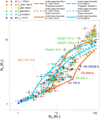 |
Fig. A.1 Same as Figure 3, but highlighting the outliers discussed in Section A. |
| In the text | |
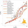 |
Fig. A.2 Same as Figure 6, but for Teq > 1350 K. |
| In the text | |
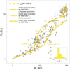 |
Fig. A.3 Same as Figure 6, but for Teq = 956 – 1350 K. |
| In the text | |
 |
Fig. A.4 Same as Figure 6, but for Teq = 680 – 956 K. |
| In the text | |
Current usage metrics show cumulative count of Article Views (full-text article views including HTML views, PDF and ePub downloads, according to the available data) and Abstracts Views on Vision4Press platform.
Data correspond to usage on the plateform after 2015. The current usage metrics is available 48-96 hours after online publication and is updated daily on week days.
Initial download of the metrics may take a while.