| Issue |
A&A
Volume 694, February 2025
ZTF SN Ia DR2
|
|
|---|---|---|
| Article Number | A12 | |
| Number of page(s) | 18 | |
| Section | Extragalactic astronomy | |
| DOI | https://doi.org/10.1051/0004-6361/202450379 | |
| Published online | 14 February 2025 | |
ZTF SN Ia DR2: Secondary maximum in type Ia supernovae
1
School of Physics, Trinity College Dublin, College Green, Dublin 2, Ireland
2
GSI Helmholtzzentrum für Schwerionenforschung, Planckstraße 1, 64291 Darmstadt, Germany
3
Univ Lyon, Univ Claude Bernard Lyon 1, CNRS, IP2I Lyon/IN2P3, UMR 5822, F-69622 Villeurbanne, France
4
Department of Physics, Lancaster University, Lancaster LA1 4YB, UK
5
Oskar Klein Centre, Department of Physics, Stockholm University, SE-10691 Stockholm, Sweden
6
Institut für Physik, Humboldt-Universität zu Berlin, Newtonstr. 15, 12489 Berlin, Germany
7
National Research Council of Canada, Herzberg Astronomy & Astrophysics Research Centre, 5071 West Saanich Road, Victoria, BC V9E 2E7, Canada
8
Institute of Astronomy and Kavli Institute for Cosmology, University of Cambridge, Madingley Road, Cambridge CB3 0HA, UK
9
IPAC, California Institute of Technology, 1200 E. California Blvd, Pasadena, CA 91125, USA
10
247-17 Caltech, Pasadena, CA 91125, USA
11
Institute of Space Sciences (ICE, CSIC), Campus UAB, Carrer de Can Magrans, s/n, E-08193 Barcelona, Spain
12
Institut d’Estudis Espacials de Catalunya (IEEC), E-08034 Barcelona, Spain
13
Lawrence Berkeley National Laboratory, 1 Cyclotron Road MS 50B-4206, Berkeley, CA 94720, USA
14
Department of Astronomy, University of California, Berkeley, 501 Campbell Hall, Berkeley CA 94720, USA
15
Department of Physics, Drexel University, Disque Hall, Office No. 808 32 S. 32nd St., Philadelphia, PA 19104, USA
16
Caltech Optical Observatories, California Institute of Technology, Pasadena, CA 91125, USA
17
Aix Marseille Université, CNRS/IN2P3, CPPM, Marseille, France
18
Oskar Klein Centre, Department of Astronomy, Stockholm University, SE-10691 Stockholm, Sweden
⋆ Corresponding author; This email address is being protected from spambots. You need JavaScript enabled to view it.
Received:
15
April
2024
Accepted:
26
June
2024
Abstract
Type Ia supernova (SN Ia) light curves have a secondary maximum that exists in the r, i, and near-infrared filters. The secondary maximum is relatively weak in the r band, but holds the advantage that it is accessible, even at high redshift. We used Gaussian process fitting to parameterise the light curves of 893 SNe Ia from the Zwicky Transient Facility’s (ZTF) second data release (DR2), and we were able to extract information about the timing and strength of the secondary maximum. We found > 5σ correlations between the light curve dec rate (Δm15(g)) and the timing and strength of the secondary maximum in the r band. Whilst the timing of the secondary maximum in the i band is also correlated with Δm15(g), the strength of the secondary maximum in the i band shows significant scatter as a function of Δm15(g). We found that the transparency timescales of 97 per cent of our sample are consistent with double detonation models and that SNe Ia with small transparency timescales (< 32 d) reside predominantly in locally red environments. We measured the total ejected mass for the normal SNe Ia in our sample using two methods and both were consistent with medians of 1.3 ± 0.3 and 1.2 ± 0.2 M⊙. We find that the strength of the secondary maximum is a better standardisation parameter than the SALT light curve stretch (x1). Finally, we identified a spectral feature in the r band as Fe II, which strengthens during the onset of the secondary maximum. The same feature begins to strengthen at < 3 d post maximum light in 91bg-like SNe. Finally, the correlation between x1 and the strength of the secondary maximum was best fit with a broken, with a split at x10 = − 0.5 ± 0.2, suggestive of the existence of two populations of SNe Ia.
Key words: surveys / supernovae: general
© The Authors 2025
 Open Access article, published by EDP Sciences, under the terms of the Creative Commons Attribution License (https://creativecommons.org/licenses/by/4.0), which permits unrestricted use, distribution, and reproduction in any medium, provided the original work is properly cited.
This article is published in open access under the Subscribe to Open model. This email address is being protected from spambots. You need JavaScript enabled to view it. to support open access publication.
1. Introduction
Although there is a general consensus that Type Ia supernovae (SNe Ia) originate from the thermonuclear explosions of white dwarfs (WDs) in binary systems, there is still some disagreement about the explosion mechanisms and progenitor scenarios (see Hillebrandt et al. 2013; Maoz et al. 2014; Ruiter 2020; Jha et al. 2019; Liu et al. 2023, for comprehensive reviews). The light curves of SNe Ia around peak light have been extensively studied because when SNe Ia are used as cosmological distance indicators (Riess et al. 1998; Perlmutter et al. 1999; Scolnic et al. 2018), they are standardised using empirical relations between the light curve shape, brightness, and colour around maximum light in the optical (Pskovskii 1977; Phillips 1993; Hamuy et al. 1996; Tripp 1998). Around two to three weeks post-maximum light, SN Ia light curves begin to rise again to a secondary bump in the optical i band and at near-infrared (NIR) wavelengths (Elias et al. 1981). A shoulder is seen in the optical r band at similar phases. This phenomenon is called the secondary maximum and it is significantly less well studied than the primary maximum due to the fainter magnitudes at these phases combined with the difficulties associated with observing in the NIR. Despite the fact it is not fully understood, the secondary maximum encapsulates important information about the physical parameters of the explosion. Dhawan et al. (2016) has shown that the secondary maximum can be used to estimate the amount of 56Ni produced in the explosion and Papadogiannakis et al. (2019a) showed the properties of the secondary maximum to be linked to the transparency timescale and total ejected mass in the explosion. Moreover, it has been shown that the secondary maximum in the i and NIR bands can be used to standardise SN Ia light curves in a similar manner as the primary maximum (Nobili et al. 2005; Shariff et al. 2016), although this does not significantly reduce the Hubble residual scatter (Shariff et al. 2016).
The secondary maximum is thought to be caused by the ionisation transition of iron-group elements (IGEs) in the ejecta from doubly to singly ionised once the ejecta temperature drops below ∼7000K. The increased NIR emissivity of singly (compared to doubly) ionised IGEs causes the NIR flux to increase (Pinto & Eastman 2000; Kasen 2006; Kasen & Woosley 2007; Dhawan et al. 2015; Hoeflich 2017). This explanation was corroborated by the identification of a strengthening Fe II spectral feature in the i band of SN 2014J (Jack et al. 2015), coinciding with the onset of the secondary maximum. Light curves that evolve more slowly and have higher peak absolute magnitudes tend to have hotter ejecta and, consequently, later secondary maxima (Kasen 2006; Blondin et al. 2015). Fainter and faster evolving SNe Ia have earlier secondary maxima (Hamuy et al. 1996; Kasen 2006; Taubenberger 2017). The existence of the secondary maximum relies on at least some level of abundance stratification, meaning that explosions with large scale mixing are not expected to show a secondary maximum (Kasen 2006). Moreover, asymmetric ejecta could lead to a viewing angle dependence in the properties of the secondary maximum (Kasen 2006). The progenitor metallicity also affects the secondary maximum through its impact on the amount of stable iron produced, with increased progenitor metallicity leading to an earlier secondary maximum (Kasen 2006).
Some of the more peculiar sub-types of SNe Ia lack a secondary maximum entirely (Turatto et al. 1996; Hoeflich et al. 2002; González-Gaitán et al. 2014; Dhawan et al. 2017; Ashall et al. 2020; Lu et al. 2021; Hoogendam et al. 2022; Dimitriadis et al. 2023). In the case of 91bg-like SNe Ia or SNe Iax, the lack of secondary maximum is explained by a very low ejecta temperature, which causes the secondary maximum to merge with the primary peak (Kasen 2006; Blondin et al. 2015; Taubenberger 2017; Galbany et al. 2019). A similar effect has been seen in the late-time light curve of 91bg-like SN 2021qvv (Graur et al. 2023), which lacks a NIR plateau. The NIR plateau occurs between 70–500 d for normal SNe Ia and is the result of a shift in the dominant ionisation state of IGEs, resembling the secondary maximum (Deckers et al. 2023). On the other extreme end of the SN Ia absolute luminosity scale, the very bright 03fg-like SNe Ia are thought to lack a secondary maximum because the secondary re-brightening is obscured by the interaction with a dense circumstellar material (CSM) or envelope (Taubenberger et al. 2011; Taubenberger 2017; Dimitriadis et al. 2021, 2023). The sub-class of 02es-like SNe Ia similarly lack a secondary maximum. Hoogendam et al. (2023) suggested that this sub-class originates from the same progenitor scenario as 03fg-like SNe Ia and that they similarly lack a secondary maximum due to interaction with a dense envelope.
Papadogiannakis et al. (2019a) studied the secondary maximum of 422 SNe Ia provided by Carnegie Supernova Project (CSP-I, Contreras et al. 2010), CfA supernova programme (Hicken et al. 2009), Palomar Transient Factory (PTF), and intermediate Palomar Transient Factory (iPTF, Rau et al. 2009). Out of these surveys, only PTF and iPTF are untargeted, which makes up about half their sample. They find correlations between the properties of the secondary maximum in the r band and sBV (a proxy for light curve stretch measured by SNooPy, Burns et al. 2014) as well as the transparency timescale (t0), which can be directly compared to predictions from explosion models, highlighting the power of the secondary maximum.
In this paper, we build upon the analysis from Papadogiannakis et al. (2019a) by performing a large scale study of the secondary maximum in the r and i bands for 893 SNe Ia provided by the Zwicky Transient Facility’s (ZTF) second data release (DR2; Rigault et al. 2025). With our large spectroscopic data set, we aim to confirm which specific spectral features are producing the secondary maximum in the r band. We also investigate whether the correlations found by Papadogiannakis et al. (2019a) between the secondary maximum and other light curve parameters hold for our larger sample. Finally, with 893 SNe Ia, DR2 contains many other sub-types beyond just normal SNe Ia, we investigated the secondary maximum properties of the more peculiar SNe Ia to test whether their properties can be connected to the normal SN Ia population through the secondary maximum as was shown by Li et al. (2022) for the transitional SN 2012ij.
In Sect. 2, we introduce the DR2 data set. We describe how we fit and analyse our light curves, introduce average spectral templates, and summarise the final samples analysed in this paper in Sect. 3. The results of our light-curve fits are presented in Sect. 4, and we provide a detailed discussion in Sect. 5. Lastly, we summarise our results in Sect. 6.
2. Data
In Sect. 2.1, we describe the ZTF DR2 dataset. In Sect. 2.2, we describe the coverage cuts we applied to ensure we only fit well-sampled light curves.
2.1. The sample
For this investigation, we used data from the ZTF survey (ZTF, Bellm et al. 2019; Graham et al. 2019; Masci et al. 2019; Dekany et al. 2020). ZTF is a large field-of-view, galaxy-untargeted transient survey that has discovered thousands of transients since first light in 2018. In particular, we investigated the second SN Ia data release (DR2; Rigault et al. 2025), which contains SN Ia data of 3628 spectroscopically confirmed events from the first three years of operations (spanning 2018–2020). An overview of the sample statistics and technical details are described in Smith et al. (2025).
We placed a redshift cut at z ≤ 0.06 because the sample is considered spectroscopically complete for normal SNe Ia up to z ≤ 0.06 (Amenouche et al. 2025). We note that the fainter sub-types in the sample will not all be discovered to this redshift (see Dimitriadis et al. 2025, for further discussion). Placing a redshift cut at z ≤ 0.06 reduces the initial sample size from 3628 to 1584 SNe Ia. Additional described in Sects. 2.1, 2.2, 3.1, 3.2, and 3.3. We summarise the final samples in Sect. 3.6 and in Table 1.
Cuts applied to produce our final sample.
2.2. Light-curve data
In this study we used light curves obtained by the ZTF survey in three optical filters (gri). We will perform Gaussian process (GP) fits to characterise these light curves, which work best when the photometry is well sampled. Therefore, we applied quality cuts to the light curve data. We required each light curve to have detections in at least two filters, with at least one of the same filter for pre- and one post-maximum light. We also required a minimum of two detections pre-peak and two post-peak in any filter, and in total a minimum of seven detections across all filters. These criteria were applied to the stacked light curves, meaning that two data points on one epoch only count as a single detection. These light curve quality criteria ensure that we are able to fit the light curves around maximum light to estimate t0x (the time of maximum in a specific filter, x). We also required a minimum of four detections between +10 and +40 d in the r band. This criterion was adopted from Papadogiannakis et al. (2019a) and ensured that we would be able to adequately constrain the secondary maximum. If there were fewer than four detections between +10 and +40 d in the i band, we kept the light curve in the sample, but we did not attempt to measure the parameters of the secondary maximum in the i band. The aforementioned light curve coverage cuts reduced the size of the sample from 1584 to 976 SNe Ia.
3. Analysis
In Sect. 3.1, we describe the GP fits to our light curves and explain our motivation for the choice of parameters (see e.g. Rasmussen & Williams 2006, for details on GP processes). In Sects. 3.2 and 3.3, we describe the parametrisation of the timing and strength of the secondary maximum, respectively, while in Sect. 3.4, we discuss the impact of K-corrections on the parameters measured here. We describe why a number of SNe Ia were cut from the sample after we inspected outliers by eye, and then summarise all the cuts we applied to arrive at the final two samples used in this analysis. Finally, we introduce a number of spectral templates we used to constrain the spectral evolution during the secondary maximum.
3.1. Fitting light curves using Gaussian processes
To characterise the evolution of the r-band light curves, we performed GP fits to the data. GPs are a data-driven, non-parametric method of estimating an underlying function behind data. The same method was implemented by Papadogiannakis et al. (2019b,a) and Pessi et al. (2021) to characterise the r- and i-band light curves of SN Ia, respectively. GPs were also used for PISCOLA (Müller-Bravo et al. 2022), a light curve fitter, and AVOCADO (Boone 2019), a photometric classifier.
We use the python package SCIKIT-LEARN to implement our GP fits, which we performed in 2D in order to fit data across different filters simultaneously. We fit the light curves in 2D to maximise the amount of data available, which helps to constrain the timing of the primary maximum (Dimitriadis et al. 2025). Our analysis focuses primarily on the r band but we also analyse the i band, which generally has less available data than the r band. By fitting the different filters simultaneously, we increased the quality of the i band light-curve fits. We fit our nightly stacked ZTF light curves in flux space so that we could include non-detections, which could not be used if we were fitting in magnitude space. An uncertainty floor of 2.5, 3.5, and 6 per cent were applied to the flux values in the g, r, and i bands, respectively (Smith et al. 2025). We fit a phase range of −15–50 d with respect to maximum light. The fluxes are normalised to peak, as is standard for GP fits to ease maximum likelihood estimation (Rasmussen & Williams 2006). An example of an average GP fit of a SN Ia in our sample is shown in the top panel of Fig. 1.
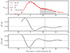 |
Fig. 1. Example of GP fit to a r-band light curve (top). The GP fit is shown as a red and the 1σ uncertainty is shown as the red shaded region. The area over which the integrated flux under the secondary maximum, ℱr2, is calculated is indicated by the grey shaded region, and t2(r) by the black dashed. The first derivative of the GP light curve (middle). This light curve has a secondary shoulder rather than a secondary maximum because the first derivative is not equal to zero. The second derivative of the GP light curve (bottom), shows that the time of the onset of the secondary maximum is the time at which the second derivative is equal to zero, also known as an inflection point. |
The choice of kernels is important for GP fitting. We tested both the radial basis function (RBF) kernel and the Matern kernel. The RBF kernel is an infinitely differentiable, stationary kernel, meaning that it produces smooth output functions (Rasmussen & Williams 2006; Duvenaud 2014), and it depends only on the distance of two data-points, which is then parameterised by a length scale parameter (ℓ), and not on their absolute values. The Matern kernel is also stationary, but it has an additional parameter, ν, which controls the smoothness of the function. The Matern kernel only produces smooth, infinitely differentiable functions at particular values of ν (Rasmussen & Williams 2006; Duvenaud 2014). We find that the Matern kernel overfits the ZTF light curves, resulting in spurious wiggles in the model. We therefore implement the RBF kernel for our GP fits. Pessi et al. (2019, 2021) also opted for a RBF kernel, whereas Papadogiannakis et al. (2019a) opted for a Matern kernel.
We tested how adding additional kernels (white noise, constant) to our GP model impacts the fits (see Fig. 2). In the top left panel of Fig. 2, we highlight that if a light curve has large gaps in the data, a GP without a white noise kernel will over-fit the data resulting in unphysical fluctuations in the flux predictions. The top-right panel of Fig. 2 shows that a GP without a white noise kernel is likely to under-predict the uncertainties, as is shown between 10–30 d. The bottom-left panel of Fig. 2 shows that excluding the constant kernel can result in deviating behaviour at the edges of the function, particularly if there is limited data in these regions. As a result of these tests, we opted to include a constant and a white noise kernel.
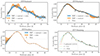 |
Fig. 2. Impact of various kernel and length scale choices on a GP fit of a ZTF SN Ia light curve. If the uncertainties in the data are underestimated, not including a white noise kernel will result in unrealistic wiggles in an attempt to fit all the points (top left). Even if the uncertainties are not underestimated in the data, a lack of a white noise kernel can result in an underestimation of the uncertainty of the GP fit, as is visible between 10–30 d in the light curve shown in the top-right panel. With limited data at the edge of the fitting regions, not including a constant kernel can result in deviating behaviour at the edge regions (bottom left). We optimise the length scale during the fit in the bottom-right panel, which in this case resulted in ℓ = 12.3 d. By setting a length scale, the likelihood is higher to either over-fit if the length scale is too short (ℓ = 3 d), or to under-fit and miss important features if the length scale is too long (ℓ = 30 d). The ideal value for the length scale will depend on the cadence of the data, which varies across our sample. |
We also tested the impact of the length scale of the time axis of the RBF kernel on the GP fits. In the bottom-right panel of Fig. 2, we show the fit for a typical event in terms of data coverage, by fixing the length scale to either a small value (ℓ = 3 d) or a large value (ℓ = 30 d). The small value results in over-fitting of the data, while the large value results in an overly smoothed function that does not capture the crucial variation of SN Ia light curves around the secondary maximum. We also show a fit where the length scale is optimised without bounds in the bottom right panel of Fig. 2. For this example event, the length scale after optimisation is 12.3 d and the fit captures the evolution of the light well without over-fitting.
Motivated by our tests, we chose to use the RBF kernel, combined with a constant and a noise kernel. We optimised the length scale of the RBF kernel for each SN, since the optimum values will depend on the cadence of each individual light curve. We found a range of length scales between 4–70 d with a median of 10 d. Upon inspection by eye, light curves with very long length scales were not well fit, so we removed any SNe Ia from our sample that are fit with a length scale > 44 d (rejecting measurements further than 3σ away from the median of the distribution). This cut removes three out of 973 SNe Ia from our sample. We implemented non-informative priors on the hyper parameters of the other kernels and ran an optimisation for each SN fit.
We estimated the uncertainties on the timing and strength of the secondary maximum (Sect. 3.2 and 3.3) by resampling. We perform 1000 iterations where we perturb the stacked flux data points within their Gaussian uncertainties and rerun the GP fits. We repeated our measurements and take the standard deviation across the 1000 iterations as the uncertainty.
3.2. Determining the time of the secondary maximum
To determine the time of the secondary maximum, we traced the GP light curves with a univariate spline and calculated the first and second derivatives. The secondary maximum is expected to occur in the range of 10–40 d with respect to maximum light (Papadogiannakis et al. 2019a). Papadogiannakis et al. (2019a) searched this range for where the first derivative is equal to zero and the second derivative is negative, which would correspond to a local maximum in the light curve. Although this would work in the i band, the secondary maximum is less prominent in the r band and it is usually better characterised as a shoulder rather than a local maximum. In order to constrain a shoulder in the r-band light curve, we located the first inflection point (where the second derivative is equal to zero, see Fig. 1) in the range 13–35 d, which we define as t2(r). We reduced the upper bound of the range from 40 d to 35 d because Papadogiannakis et al. (2019a) found no secondary maxima later than 35 d; we find that there is often limited data at this range, which can result in an unexpected behaviour of the GP function. We reject any measurements of t2(r) with an uncertainty more than 3σ away from the median of the uncertainty distribution (σt2 > 5.9 d), to eliminate objects with poor GP fits, which removes 45 SNe Ia.
We found 20 91bg-, seven 02cx-, and three 02es-like SNe Ia (including SN 2019yvq), with t2(r) > 20 d. These sub-types are not expected to show strong, late secondary maxima, making them stand out significantly from the rest of the sample. We checked all their light curves by eye and found that their light curves flatten as they approach zero flux around 20 d. Because the absolute flux is very low at these epochs, small fluctuations are picked up in the derivatives and can be classified as inflection points, but these are not a real secondary shoulders or maxima. This is not a problem for most of the normal SNe Ia in the sample because they decline less rapidly and, therefore, they do not have such low flux values in the window where we search for the secondary maximum. Because the light curves of these objects are well fit by the GP function, we did not remove these SNe Ia from our sample; instead, we only remove their measured t2(r) values. The only exceptions are SN 2018jpk (an 02cx-like SN Ia) and SN 2019ner (an 02es-like SN Ia), which do appear to have a real secondary maximum at 20.9 and 20.6 d, respectively. We kept both of their t2(r) values in the sample.
Our t2(r) values are better described as the onset of the shoulder, rather than the peak of the secondary maximum (see Fig. 1). Papadogiannakis et al. (2019a) also measured the inflection point, but only for light curves, where they could not locate a true secondary maximum (dF/dt = 0). We opted to use the point where d2F/dt2 = 0 (inflection point) for all light curves to ensure we are consistent across the sample because we are interested in relative t2(r) values. We were able to find a secondary maximum for 808 SNe Ia, and 60 of these could be characterised as having a true bump (dF/dt = 0)1. A direct comparison of our t2(r) values to those presented in Papadogiannakis et al. (2019a) is hindered by the fact that they do not specify which t2(r) values correspond to dF/dt = 0 vs. d2F/dt2 = 0.
In Fig. 3, we highlight the importance of using a consistent definition of t2(r). We measured t2(r) only for SNe Ia with an identified bump (dF/dt = 0), using both methods. We find that the median difference between the inflection point d2F/dt2 = 0 and the local maximum in the light curve (dF/dt = 0) is 1.9 d, with the inflection point generally occurring earlier.
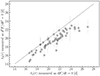 |
Fig. 3. Distribution of t2(r) for the 63 SNe Ia with a detected true bump (i.e. dF/dt = 0 exists), measured either as the local maximum (dF/dt = 0, x-axis) or the inflection point (d2F/dt2 = 0, y-axis). We systematically find a lower t2(r) if measured as the point of inflection versus the local maximum in the light curve. |
We also measured t2 using the inflection point (d2F/dt2 = 0) for the i band (t2(i)). We find that 103 of the i band light curves could be characterised as having a true bump (dF/dt = 0). This is more than in the r band, which is not surprising because the secondary maximum is known to be stronger in the i band. The median offset between the point at which dF/dt = 0 and d2F/dt2 = 0 is 4.6 d, which is larger than in the r band. This is because the secondary maximum is more prominent and lasts longer in the i band (see Fig. 10, Kasen 2006). As a result, the time between the onset and the peak of the secondary maximum is greater.
3.3. Constraining the strength of the secondary maximum
We used the integrated flux under the secondary maximum, ℱr2, to quantify the strength of the secondary maximum (see shaded region in the top panel of Fig. 1). The same metric was used in Krisciunas et al. (2001) and Papadogiannakis et al. (2019a) to quantify the strength of the secondary maximum in the i and r bands, respectively. ℱr2 was calculated by normalising the flux to peak in the r band, integrating the flux between +15 and +40 d (where rest-frame phase is defined relative to peak in the r band) and dividing by the length of the interval (25 d). We rejected any measurements of ℱr2 with an uncertainty more than 3σ away from the median of the uncertainty distribution (σℱr2 > 0.05) to eliminate objects with poor GP fits, thus removing 30 SNe Ia.
3.4. Uncertainties due to K-corrections
At high redshifts, it is important to apply K-corrections because the observed r-band will begin to resemble rest-frame g-band, where no secondary maximum is expected. Unfortunately, this is not straightforward due to a lack of reliable templates at the phases we are investigating (+15 to +40 d post peak). Moreover, some of the more peculiar sub-types present in our sample do not have sufficient template coverage to calculate reliable K-corrections at any phases.
We estimated the impact of K-corrections using the SALT3 (Spectral Adaptive Light-curve Template; Kenworthy et al. 2021) template in the SNCOSMO library (Barbary et al. 2022). We produced a grid of light curves which resemble the normal SNe Ia in our sample, with −3 ≤ x1 ≤ 3 in steps of 0.5 and −0.2 ≤ c ≤ 0.8 in steps of 0.1. We placed these light curves at a range of redshifts (0 ≤ z ≤ 0.06). Next, we measured t2(r) and ℱr2 for all the simulated light curves and find how much the values differ compared to the simulated light curve with the same x1 and c at z = 0 (see Fig. 4). We adopted the residuals as additional uncertainties due to unaccounted for K-corrections in our measured parameters (t2(r/i), ℱr2/i2). We selected the grid residual point that we would adopt for each SN based on its redshift, x1, and c in bins of 0.01, 0.5, and 0.1, respectively. The measured x1- and c-values are not always reliable for the SNe Ia that are not in our cosmological sample (see Sect. 3.6); nonetheless, we use them here to obtain a rough estimate of the additional uncertainty due to K-corrections that were unaccounted for.
 |
Fig. 4. Impact of K-corrections on t2(r) (top) and ℱr2 (bottom), as a function of redshift and x1 (left) and c (right). The colour of the data points represents the residual between the measured parameter in the SALT3 model at that point and the same model at z = 0. Overall, the impact of K-corrections is small, with a maximum residual on ℱr2 of 0.014 and on t2(r) of 0.66 d. |
The variation over the redshift range covered by our sample is < 0.66 d for t2(r), < 0.20 d for t2(i), < 0.014 for ℱr2, and < 0.087 for ℱi2, suggesting that the impact of K-corrections on our results is minimal. As a sanity check, Fig. 4 also check how the measured parameters vary for the Hsiao template (Hsiao et al. 2007) compared to the SALT3 template with x1 = 0 and c = 0. Although the absolute values of the measured parameters differ from those measured from SALT3, the deviation with redshift is comparable.
3.5. Outlier rejection
Although we tried to ensure only good quality GP fits are included in our sample by applying a number of cuts detailed in the previous sections, a few poor fits are still present. Due to the large sample size, we only inspected the light curves and GP fits for SNe Ia with extreme t2(r) or ℱr2 values by eye. As a result of these manual inspections, we removed a few objects from our sample.
SN 2018but (a normal SN Ia) was removed because the GP function showed an unrealistic extrapolation due to a lack of data at > 30 d. SN 2019sua (91bg-like) was removed because the data between 20–50 d showed spurious fluctuation with underestimated uncertainties, which resulted in unrealistic wiggles in the GP fit. Three additional SNe Ia were removed (SNe 2018ggw, 2020bxp, and 2020acol, all three normal) because their GP fits produce a dip in the light curve around 20 d even though there is no data in any band. After removing these additional five SNe Ia, the final sample contains 893 SNe Ia.
3.6. Summary of final samples
We provide a summary of the various cuts applied in Sects. 2.1, 2.2, 3.1, 3.2, and 3.3, and the outliers removed in this section that were used to arrive at our main sample and cosmological sample that was presented in Table 1.
Our final sample consists of 893 SNe Ia. Although the sample is dominated by normal SNe Ia (706), there are many sub-types of SNe Ia present. The most ubiquitous are the over-luminous 91T-like SNe Ia (56), followed by sub-luminous 91bg-like SNe Ia (36). A full break-down of the various sub-types is shown in Table 2, and a more detailed analysis of the various sub-types and their rates in DR2 will be presented in Dimitriadis et al. (2025).
SN Ia sub-types present in our final sample.
In this study, we used the decrease in magnitude between peak and +15 d in the g band, Δm15(g), as a measure of the stretch of a light curve. We adopted the Δm15(g)-values from Dimitriadis et al. (2025), which are estimated after K-correction using GP fits to the light curves. SALT2 based K-corrections are applied to normal and 91T-like SNe Ia, template K-corrections are applied to all other sub-types, apart from Ia-CSM, which have no applied K-corrections (see Dimitriadis et al. 2025, for further discussion). We also aimed to perform comparisons between our parameters and those presented in other DR2 cosmology papers, which implement x1 and c measured using SALT2.4 (Guy et al. 2007; Taylor et al. 2021). SALT2.4 is trained predominantly on templates of normal SNe Ia and can therefore not accurately measure the light curve parameters for more peculiar SNe Ia. We therefore defined a ‘cosmology’ sub-sample on the basis of the same cuts as those implemented by Rigault et al. (2025) for the cosmological analysis of the DR2 sample (i.e. x1 and c: |x1|< 3, −0.2 ≤ c ≤ 0.8, cuts on the uncertainties of |σx1|≤1, |σc|≤0.1, |σt0|≤1, a fit-probability > 1e−7, and either no sub-classification, or a sub-classification of normal, 91T- or 99aa-like). These cuts result in a sub-sample of 783 SNe Ia. We distinguish this sub-sample from our main sample by referring to it as our cosmological sub-sample because it adheres to the cuts normally applied in order to perform cosmological analysis. However, we note that the DR2 is currently not suitable for inferring cosmological parameters (see Rigault et al. 2025, for further discussion).
3.7. Averaged spectral templates
In this paper, we are interested in constraining the spectral properties of SNe Ia from maximum light with the aim of understanding the spectral features contributing before, during, and after the time of secondary maximum (e.g. from peak to +30 d). To investigate this, we have compiled average spectral templates as a function of x1 and phase from a sample of SN Ia spectra from the ZTF DR2 cosmological sub-sample (Burgaz et al. 2025; Johansson et al. 2025), supplemented with additional spectra taken by ZTF post-DR2 (obtained between February 2021 – September 2023) along with literature spectra obtained from WISEREP. The additional spectra were used to increase the sample size at the upper and lower ends of our x1 range at later phases (+15 to +30 d).
We excluded spectra with a signal-to-noise ratio (S/N) in the continuum of < 5, and we binned the spectra to 10 Å resolution to account for varying resolution across the sample, in particular the low resolution spectra (R ∼ 100) taken by the SEDMachine (Rigault et al. 2019; Blagorodnova et al. 2018; Kim et al. 2022). In total, we include 265 spectra of SNe Ia in our cosmological sub-sample, where the phase is defined relative to the time of maximum in the g band from the SALT2.4 fit. We also included 9 SN Ia spectra taken by ZTF post-DR2 at z ≤ 0.06 at phases between +10 and +40 d. We fit the light curves of SNe Ia obtained post-DR2 with SALT2.4 using the same procedure as for the rest of the sample to obtain x1 and t0 values. Finally, we searched WISEREP for spectra taken between +10 and +40 d for normal SNe at z ≤ 0.06 and with published x1 and t0 values, adding a further 17 spectra. These additional spectra were pre-processed in the same way as the ZTF DR2 spectra.
In Fig. 5, we show the r- and i-band region of the averaged spectra of SNe Ia from our cosmological sub-sample, sorted into two x1 bins (−3 ≤ x1 < 0 and 0 ≤ x1 < 3), and six phase bins (0–10, 10–20, 20–30, 30–40, and 40–50 d). The spectra in each bin were first sigma-clipped (5σ), then averaged, and finally smoothed with a Gaussian convolution with a standard deviation of 5. All averaged spectra are then normalised to the continuum region at 7000 Å. We also include spectra of SN 1999by (a 91bg-like SN Ia, Matheson et al. 2008) taken from WISEREP in the bottom panel of Fig. 5. The spectra of SN 1999by are also normalised to the continuum region around 7000 Å.
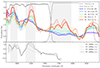 |
Fig. 5. Averaged spectra between 0–10, 10–20, 20–30, 30–40, and 40–50 d in the r- and i-band wavelength ranges. The phases are relative to g-band maximum. Spectra are binned into −3 ≤ x1 < 0 (dashed) and 0 ≤ x1 < 3 (solid). The grey shaded regions indicate the spectral regions where a feature appears during the onset of the secondary maximum. The numbers in the brackets represent the number of spectra going into each bin (first number represents the number of spectra in the −3 ≤ x1 < 0 bin, and the second number are the number of spectra in the 0 ≤ x1 < 3 bin). We also show the filter response functions of the ZTF r and i bands in black. In the bottom panel we show a spectral timeseries of SN 1999by (a 91bg-like SN Ia). |
4. Results
After the additional cuts on the length scale and uncertainties on t2(r) and ℱr2, as well as the removal of outliers, the main sample remaining consisted of 893 SNe Ia. In this section, we test whether the correlations found by Papadogiannakis et al. (2019a) for the CfA and CSP samples persist for our sample. We then analyse the available spectra in order to constrain the spectral feature responsible for the secondary maximum in the r band. Next, we use the integrated flux under the secondary maximum to estimate the transparency timescales for the SNe Ia in our main sample, and compare it to model predictions. We also provide estimated total ejected masses derived from the transparency timescale and compare them to the masses derived from the SALT2.4 light curve width parameter, x1, for our cosmological sub-sample.
4.1. Timing and strength of secondary maximum
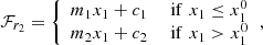
We measured the timing and the strength of the secondary maximum for the r and i band. All four parameters, t2(r), t2(i), ℱr2, and ℱi2, are shown as a function of Δm15(g) in the four panels of Fig. 6.
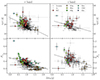 |
Fig. 6. Timing of secondary maximum (t2(x), top) and normalised integrated flux in the range of 15–40 d (ℱx2, bottom) in the r band (left) and i band (right) as a function of Δm15(g) for our sample. We also show simple linear regression fits to the whole sample (black dashed lines). We find a non-zero slope at the > 5σ confidence level for t2(r), t2(i), ℱr2, but not for ℱi2 with Δm15(g). |
4.1.1. r band
We measured the timing of the secondary maximum (shoulder) in the r band, t2(r), for our ZTF sample and find values ranging between ∼13–34 d with respect to maximum light. This is similar to the range seen in Papadogiannakis et al. (2019a), but our values are slightly smaller due to the different definition of t2(r) (see Sect. 3.2).
In the top panel of Fig. 6, we show t2(r) as a function of Δm15(g). We find a strong correlation for the normal SN Ia population, with a Pearson correlation coefficient r of −0.69 at a > 5σ confidence level. Papadogiannakis et al. (2019a) found the timing of the secondary maximum to correlate with SNooPy light-curve width parameter, sBV, which itself is strongly correlated with Δm15(B) (Burns et al. 2018). We were able to measure t2(r) for a number of unusual classes of SNe Ia (also shown in Fig. 6), and find that they broadly follow the normal sample relation. The correlation between t2(r) and Δm15(g) becomes weaker but remains statistically significant when tested for the whole sample rather than just the normal SNe Ia (Pearson correlation coefficient r of −0.60 at a > 5σ confidence level).
There are 7, out of a total of 46, 91bg-like SNe Ia with an identified t2(r), which is unexpected because this sub-class is characterised by a lack of secondary maxima (e.g. Taubenberger 2017). We inspected all their light curves by eye and for six out of seven, their secondary maxima look real (i.e. there is sufficient data to constrain a secondary maximum and all data points around t2(r) are consistent with the GP fit, and if i-band data is available t2(r) agrees with t2(i) within 3σ). We removed the t2 measurements of SN 2020acbx from the sample because t2(i) is not coincident with t2(r) within 3σ. Furthermore, we found a secondary maximum for SN 2018jpk, which is a 02cx-like SNe Ia. The 02cx-like sub-class are not expected to have secondary maxima due to their well-mixed ejecta composition (Jha 2017). We find one SN Ia-CSM (SN 2020ue; Sharma et al. 2023) with a late secondary maximum (t2(r) = 31.6 d). Although the secondary maximum looks real, it is possible that this increase in flux in the light curve is fuelled by the interaction with the CSM rather than recombination of IGE because the light curve remains approximately flat for ∼50 d.
We measured the normalised integrated flux under the secondary maximum (ℱr2), which we used as a measure of the strength of the secondary maximum. The typical range of ℱr2 for the normal SNe Ia in our sample is 0.20–0.55, which deviates slightly from what was found by Papadogiannakis et al. (2019a) of 0.25–0.60. In Fig. 7 we compare the distributions of ℱr2-values between the two samples and find that the ZTF DR2 population peaks at lower values, with the medians of the two distributions differing by 0.1. We do not expect any intrinsic difference between the SN Ia samples. However, the integrated flux under the secondary maximum was originally defined as a parameter by Krisciunas et al. (2001) to quantify the strength of the secondary maximum in the i band. Krisciunas et al. (2001) integrated over the range 20–40 d, and normalised by dividing the integral by 20 d. Although Papadogiannakis et al. (2019a) described their integration as over the same range as this paper (15–40 d), if we divide our integrals by 20 d instead of 25 d, the ℱr2 distribution from ZTF lines up very well with that of PTF and iPTF (the shifted distribution is also shown in Fig. 7). As a sanity check, we compare our ℱi2-values to those presented in Krisciunas et al. (2001) and they cover the same range, whereas those presented by Papadogiannakis et al. (2019a) are offset to higher ℱi2-values, just as their ℱr2-values are.
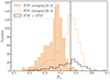 |
Fig. 7. Histogram showing the distribution of ℱr2 for the ZTF DR2 sample with the flux integral divided by 25 d (shaded orange) or divided by 20 d (dashed orange), compared to the distribution found for PTF and iPTF by Papadogiannakis et al. (2019a) (black). The median of the PTF+iPTF population is 1.5σ higher than the median of the ZTF DR2 population when the integral is divided by 25 d, but the ZTF distribution is consistent with the PTF+iPTF distribution if the integral is divided by 20 d instead. |
The bottom panel of Fig. 6 shows ℱr2 as a function of Δm15(g), and we also find a very strong correlation between these parameters for the normal SN Ia population, with a Pearson correlation coefficient r of −0.72 at a > 5σ confidence level. ℱr2 is a useful metric because we are able to measure it for all the light curves in our sample, not just those with a measured secondary maxima. This means we are able to include sub-types of SNe Ia which typically do not show a secondary maximum. When measured for the full sample, the strong correlation remains (a Pearson correlation coefficient r of −0.71 at a > 5σ confidence level).
The most distinct outlier visible in the bottom panel of Fig. 6 is a Ia-CSM, which sits 21σ above the trend. In general, the 03fg-like sub-class also have larger ℱr2 than expected for their Δm15(g) value. Since both these sub-classes of SNe Ia are thought to be powered by some interaction with a dense envelope/CSM (Taubenberger et al. 2011; Taubenberger 2017; Dimitriadis et al. 2021, 2023; Sharma et al. 2023), a higher ℱr2 is expected. Some of the 02es-like SNe Ia also sit above the trend, implying a higher than expected ℱr2. Hoogendam et al. (2023) suggested that this sub-class is linked to the 03fg-like sub-class because the two share similar photometric and spectroscopic properties. Interaction with a dense envelope could also explain the higher ℱr2 for the 02es-like sub-class. We note that all three of these sub-classes show a range of ℱr2-values, with the majority having larger ℱr2-values than normal SNe Ia, but some are consistent with the normal population.
There is a spread in the ℱr2 values of the 02cx-like sub-class, with most being consistent with the general trend, but several sitting slightly above the trend. 02cx-like SNe Ia are thought to leave behind a bound remnant which could explain the additional flux at these phases (Kromer et al. 2013a; Jha 2017).
The mean ℱr2 for the 91T-like sub-class is 0.41, whereas the mean ℱr2 for normal SNe Ia in the same Δm15(g) range (0.3 ≤Δm15(g) ≤ 1.05) is 0.37. Leloudas et al. (2015) suggested the brighter peak absolute magnitudes of the 91T-like sub-class can be attributed to interaction with a dense CSM originating from a non-degenerate companion. The ℱr2-values we find for this sub-class can be interpreted to support this proposition if we assume that the additional flux from the interaction contributes more in the period between 15-40 d, than it does at peak, since ℱr2 is calculated from the peak normalised light curves. SN 2020uoo has a weak secondary maximum (ℱr2 = 0.30), but we note that although the GP fit quality is good, this SN passed our light curve coverage criteria due to having sufficient i-band data on the rise, but it has limited g- and r-band data, which could result in a biased estimate of the time of maximum light and therefore Δm15(g). This is unusual since in most cases, ZTF light curves have significantly more data in g and r than i.
It is notable that the 91bg-like SNe Ia appear like a continuous extension of the normal SN Ia population in the bottom left panel of Fig. 6, since there is ongoing debate as to whether 91bg-like SNe Ia have a different physical origin from normal SNe Ia (Taubenberger et al. 2008; Li et al. 2022; Graur 2023; Harvey et al. 2023). Based solely on the behaviour of ℱr2 as a function of Δm15(g), it appears that 91bg-like and normal SNe Ia are members of the same population.
4.1.2. i band
We find that the timing of the secondary maximum is broadly consistent between the r and i band (see Fig. 8), suggesting that the secondary maximum in the two filters share a common cause. The correlation we found between Δm15(g) and t2(r) persists for the i band (see top right panel of Fig. 6), with a Pearson correlation coefficient r of −0.45 at a > 5σ confidence level for the normal population, and a Pearson correlation coefficient r of −0.34 at a > 5σ confidence level for the full sample. This is slightly weaker than the correlation in the r band, but there are many fewer SNe with sufficient i-band data to fit the secondary maximum.
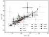 |
Fig. 8. t2(r) vs. t2(i). We also show a simple linear regression fit (black dashed line) through the full data set.t2(r) vs. t2(i). We also show a simple linear regression fit (black dashed line) through the full data set. |
We also compare ℱi2 to ℱr2, and find that ℱi2 is higher than ℱr2 for the majority of the sample (174 out of 182 that could be fitted in the i band), as was found by Papadogiannakis et al. (2019a). Since the secondary maximum is known to be stronger in the i band than in the r band, a higher integrated flux in this phase range is expected.
The strong correlation between ℱi2 and Δm15(g) does not persist for the i band, shown in the bottom right panel of Fig. 6, where we find r = −0.27 at a > 5σ confidence level for the full sample and no significant correlation at all for the normal population alone. The 91T-like SNe Ia in particular show a wide spread of ℱi2 values (0.18 ≤ ℱi2 ≤ 0.85 vs. 0.28 ≤ ℱr2 ≤ 0.47, although we note that the uncertainties are larger in the i band due to the poorer data coverage). Further discussion of the potential causes of the differences in the r and i bands can be found in Sect. 5.1.
4.2. Spectral features causing the secondary maximum
Jack et al. (2015) identify Fe II as the dominant spectral feature that causes the secondary maximum in the i band. Their models produce Co II lines and blended Fe II features (at 6900 Å and 7500 Å) in the r band, which strengthen around the time of the secondary maximum. However, these features alone are not sufficient to explain the increase in flux during the r-band shoulder. There is another feature around 6500 Å in the spectra of SN 2014J presented by Jack et al. (2015, see their fig. 8), which their model was not able to reproduce.
We can see from Fig. 5, which shows the r- and i-band wavelength range of averaged spectra of SNe Ia from our cosmological sub-sample, that there is an emission feature in the r band, red-ward of Si II 6355 Å around 6500 Å, which become stronger in SNe Ia with narrower light curves (−3 ≤ x1 < 0) as early as 10–20 d after peak. In SNe Ia with broader light curves (0 ≤ x1 < 3) this occurs later, around 20–30 d after peak. The flux values are dependent on the region used to normalise the spectra, but the line profiles are similar in the r-band region from ∼20 d onwards. Since t2(r) scales with x1 (see Sect. 4.1), we suggest that the appearance of these features play a dominant role in the secondary maximum in the r band, just like the Fe II feature identified by Jack et al. (2015) causes the secondary maximum in the i band. There is an additional spectral feature blue-ward of Si II 6355 Å around 5850 Å, which appears to decrease in strength between 10–30 d, but then gets stronger and finally peaks in strength between 40–50 d. However, due to the limited number of spectra in these final bins, and because the spectra of SN 2014J presented by Jack et al. (2015) also showing a decreasing flux in this region, we do not trust that this feature plays a dominant role in the appearance of the secondary maximum. In the i band region of the top panel of Fig. 5 we also clearly see the broad Fe II feature (between 7200–8000 Å) which was previously identified by Jack et al. (2015). This feature increases in strength between 10–40 d, and per each phase bin, it is stronger for spectra of SNe Ia with smaller x1 values.
In Fig. 9, we show the breakdown of species contributing to each feature for a non local thermodynamic equilbrium (NLTE) radiative transfer model using ARTIS of a W7 explosion model (Nomoto et al. 1984; Shingles et al. 2020, 2022) at 30, 40, and 50 d post explosion (approximately 12, 22, and 32 d past maximum light). From this model, it appears that the predominant IGE contributor to the feature at ∼6500 Å (which is similar to the unidentified feature in SN 2014J, Jack et al. 2015) is Fe II. The feature that sits blue-ward of Si II (around 5850 Å) has a strong contributions of Co III and Fe III which fade away as recombination occurs, explaining why this feature initially fades. Although the region also shows a presence of Fe II which get stronger as time progresses, the relative strength of the Fe II in this spectral feature compared to that at 6500 Å is weaker. The growing contribution of Fe II in the i band region between 7200–8000 Åis also clearly visible in these models. We use the W7 model since it has been shown to be able to reproduce a secondary maximum in the i band and a secondary maximum in the r band (Jack et al. 2011). However, the choice of assumed explosion model can affect the relative contributions of each ion to the net spectrum and therefore, these line identifications are not entirely reliable.
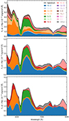 |
Fig. 9. Spectra showing the breakdown of species contributing to each feature from a NLTE radiative transfer model of the W7 explosion model at 30 d (top), 40 d (middle), and 50 d (bottom) past explosion. |
One of the defining photometric characteristics of 91bg-like SNe Ia is their lack of secondary maxima (Hoeflich et al. 2002; González-Gaitán et al. 2014; Dhawan et al. 2017; Ashall et al. 2020; Hoogendam et al. 2022). It has been argued that these faint events are faster evolving because they have cooler ejecta, enabling recombination to occur sooner, shifting their secondary maximum to earlier times, causing it to blend with the primary maximum (Kasen 2006; Blondin et al. 2015; Taubenberger 2017). We included spectra of SN 1999by (which is a 91bg-like SN Ia) in the bottom panel of Fig. 5. The feature we have tentatively classified as Fe II, which coincides with the onset of the secondary maximum in normal SNe Ia, starts to come through in the spectra of SN 1999by as early as ∼3 d post maximum light. This is significantly earlier than for the normal SNe Ia with narrow light curves (−3 ≤ x1 < 0) shown in the top panel of Fig. 5. In the future, we aim to get more detailed spectroscopic time series of 91bg-like SNe Ia to determine the range of phases at which the recombination occurs for this sub-class.
4.3. Transparency timescale
The transparency timescale is defined by Jeffery (1999) as the epoch at which the ejecta have an optical depth of unity to γ-rays. For normal SNe Ia, this value ranges between 30–50 d (Scalzo et al. 2014; Dhawan et al. 2018). The transparency timescale is a valuable metric because it has been shown to relate directly to the total ejected mass (Jeffery 1999; Stritzinger et al. 2006a; Scalzo et al. 2014; Dhawan et al. 2018, 2017), which can be used to constrain the explosion models for SNe Ia.
Papadogiannakis et al. (2019a) were able to calculate pseudo-bolometric light curves for SNe Ia in their sample provided by CSP because these have multi-wavelength coverage. From the pseudo-bolometric light curves they calculate the transparency timescale (t0). They compare their values of t0 for the CSP sub-sample to their measured t2(r) and ℱr2 values, and find a strong correlation with the latter, providing the following linear relation:
 (1)
(1)
relating ℱr2 to t0. Due to the offset in our ℱr2 distribution compared to that presented in Papadogiannakis et al. (2019a), see Sect. 4.1, we cannot directly use the above linear correlation to estimate t0 for our sample. Instead, we recalculate ℱr2 by dividing the integrated flux between 15–40 d by 20 d (which we will refer to as  ), ensuring that the distribution matches that of Papadogiannakis et al. (2019a) as shown in Fig. 7.
Using Eq. 1 and  , we estimate the t0 values for our sample. In the top panel of Fig. 10 we show the distributions of t0 for the cosmological SN Ia sample (see definition in Sect 3.6). The t0 distribution does not show a single Gaussian distribution but instead appears bimodal, with a stronger peak at longer t0 than the weaker peak at shorter t0 values. This is similar to the bimodal x1 distribution identified in Nicolas et al. (2021) and Ginolin et al. (2024).
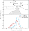 |
Fig. 10. Distributions of transparency timescales for the whole cosmological sub-sample are shown at the top (grey), along with a bimodal Gaussian fit (solid grey line) and its individual components (dashed grey). The arrows show the ranges of transparency timescales predicted by doubledet_2010 (Fink et al. 2010; Kromer et al. 2010), doubledet_2020, (Gronow et al. 2020), doubledet_2021(Gronow et al. 2021), ddt_2010 (Fink 2010), ddt_2013 (Seitenzahl et al. 2013; Sim et al. 2013), ddt_2014 (Ohlmann et al. 2014), SCH, PDDEL, and DDC (Blondin et al. 2017) explosions models. In the bottom plot we separate the transparency timescale distribution into SNe Ia with blue local colours ((g − z)local ≤ 1.0, blue) or red local colours ((g − z)local > 1.0, red). We show bimodal Gaussian the fits to both distributions, and the individual components making up the fit are shown as dotted lines. The Akaike Information Criterion (AIC) test prefers a bimodal fit for the SNe Ia in red local environments, but it does not show a preference for either the double component fit or single component fit for the SNe Ia population in blue environments, so we also show the single component fit as a dashed line to this population. |
To estimate the properties of this bimodal distribution, we fit the t0 values with a double Gaussian model. The fit is defined as P(t0) = r𝒩(μhigh, σhigh)+(1 − r)𝒩(μlow, σlow), where P(t0) is the probability distribution, 𝒩 is the Gaussian distribution, r is the amplitude of the high t0 Gaussian, μ is the mean and σ is the standard deviation of each Gaussian. We summarise the results of this fit in Table 3. We find r = 0.74 ± 0.05, suggesting that the higher t0 mode is the dominant mode over those SNe Ia with lower t0 values. This result is consistent with what was found for the bimodal x1 distribution in Nicolas et al. (2021) (r = 0.755 ± 0.05), but not with Ginolin et al. (2024) (r = 0.60 ± 0.07).
We also compare the distribution of t0 in our sample to theoretical explosion models, akin to Fig. 5 in Papadogiannakis et al. (2019a). We fit the following energy deposition function to the bolometric light curves:
![Mathematical equation: $$ \begin{aligned} E_{\rm dep}&= \lambda _{\rm Ni} N_{\rm Ni} Q_{\mathrm{Ni}, \gamma } \exp {(- \lambda _{\mathrm{Ni}} t}) \nonumber \\&\quad +\ \lambda _{\mathrm{Co}} \frac{\lambda _{\mathrm{Ni}}}{\lambda _{\mathrm{Ni}} - \lambda _{\mathrm{Co}}} [\exp {(-\lambda _{\mathrm{Co}} t}) - \exp {(-\lambda _{\mathrm{Ni}} t})] \\&\quad \times \ [Q_{\mathrm{Co}, e^+} + Q_{\mathrm{Co}, \gamma } (1 - \exp {((-t/t_0)^2)})],\nonumber \end{aligned} $$](/articles/aa/full_html/2025/02/aa50379-24/aa50379-24-eq4.gif) (2)
(2)
where λNi and λCo are the inverse of the e-folding times of nickel and cobalt (1/8.8 and 1/111.3 d−1, respectively), NNi represents the number of nickel atoms present, which is calculated from the mass of 56Ni, which is derived from the peak of the bolometric light curve (Arnett 1982). QNi, γ and QNi, γ represent the energy released from γ-ray decays of 56Ni → 56Co and 56Co → 56Fe, respectively (1.75 and 3.61 MeV) and QNi, e+ is the energy release of the positron decay of 56Co → 56Fe (0.12 MeV).
We considered two types of explosion models from the Heidelberg Supernova Model Archive (HESMA; Kromer et al. 2017), double detonation and delayed detonation models. Specifically, we included the ranges predicted by doubledet_2010 (Fink et al. 2010; Kromer et al. 2010), doubledet_2020, (Gronow et al. 2020), doubledet_20212 (Gronow et al. 2021), ddt_2010 (Fink 2010), ddt_2013 (Seitenzahl et al. 2013; Sim et al. 2013), and ddt_2014 (Ohlmann et al. 2014). The t0 ranges predicted by these models are shown in the top panel of Fig. 10. We also include model predictions from Blondin et al. (2017) for pure central detonations of sub-Mch WDs (SCH), pulsational Mch delayed-detonations (PDDEL), and standard Mch delayed-detonations (DDC). We checked the t0 distributions for gravitationally confined detonation (Seitenzahl et al. 2016; Lach et al. 2022) and merger models (Pakmor et al. 2010, 2012; Kromer et al. 2013b, 2016), but the shortest t0 value produced by these models was 45 d and their t0 values extended out to 70 d, which is not consistent with any of our observations.
We find that the t0 predictions from the doubledet models are consistent with 97 per cent of our cosmological sub-sample, whereas only 28 per cent are consistent with the predictions from the ddt models. From the models presented by Blondin et al. (2017), the t0 values predicted by the SCH models are consistent with the largest percentage of our sample (26 per cent). The other two explosion models, DDC and PDDEL, are consistent with equal percentages of the sample (8 per cent).
We also checked which explosion model t0 predictions are most consistent with the common SN Ia sub-types. The 91bg-like sub-class spans 22.2 ≤ t0 ≤ 35.3 d with a median of 26.1 d, and the 91T-like sub-class spans 31.0 ≤ t0 ≤ 41.7 d with a median of 38.1 d. None of the 91bg-like SNe Ia are consistent with the predictions from the ddt explosion models, 18 per cent are consistent with the doubledet explosion models, and only 3 per cent are consistent with the SCH explosion models. On the other hand, 100 per cent of the transparency timescales of the 91T-like SN Ia population are consistent with the doubledet, 76 percent are consistent with ddt, 40 per cent are consistent with both PDDEL and DDC, and only 3 per cent are consistent with the SCH explosion models.
To test whether the low t0 component originates from SNe Ia in particular host galaxy environments, we binned the distribution into locally blue or red environments ((g − z)local ≤ 1.0 or (g − z)local > 1.0, as shown in the bottom panel of Fig. 10). We fit the resulting two distributions with either a single or bimodal Gaussian, the only priors being that the amplitudes of the Gaussians cannot be negative and they cannot share the same mean. We used the Akaike information criterion (AIC, Burnham & Anderson 2004), which is a good test for comparing models because it penalises for additional parameters, to determine whether the population is better described by a single or double component Gaussian. We find that the SNe Ia in locally blue environments can be fit by either a single or double component, with the AIC values differing by < 2, which is the standard cut-off point for determining whether one model is preferred over the other (Burnham & Anderson 2004). The distribution of SNe Ia in locally red environments on the other hand shows a strong preference for two components, with an AIC value 39 units lower than for the single component fit.
4.4. Total ejected mass
One of the strongest constraints for different progenitor scenarios is the total ejected mass (Mej), since most explosion scenarios can be placed in one of two categories: Mch or sub-Mch. Unfortunately, we cannot calculate the total ejected mass directly since this requires bolometric light curves (e.g. Arnett 1982; Jeffery 1999), which are not available for the ZTF sample where we only have g, r, and i coverage.
However, we can use our t0 values (which were derived from  ) to estimate Mej using the equation;
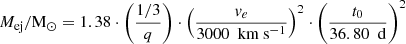 (3)
(3)
which was presented in this form by Papadogiannakis et al. (2019a) but originally derived by Jeffery (1999). In Eq. (3), q is a qualitative description of the distribution of the material of the ejecta (a high value for q implies a more centrally concentrated ejecta) and ve is the e-folding velocity assuming an exponential density profile. We adopt the same values as Papadogiannakis et al. (2019a): q = 1/3 and v2 = 3000 km s−1, leaving t0 as the only variable. These assumed values are approximately valid for normal SNe Ia, with more or less luminous SNe Ia having higher or lower e-folding velocities, respectively. We calculate Mej for the SNe Ia in our cosmological sub-sample using the t0 values calculated in Sect. 4.3 (see Fig. 11). Although they are a member of the cosmological sub-sample, we highlight the 91T-like SN Ia population in Fig. 11, which sit at the upper end of the Mej distribution. We also present the calculated Mej-values for the 91bg-like population in Fig. 11, but because the assumptions on q and ve are not necessarily valid for this sub-populations, their measured ejecta masses may be less accurate.
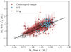 |
Fig. 11. Comparison between the total ejected mass derived from |


Scalzo et al. (2014) studied SNe Ia with multi-wavelength coverage (enabling the construction of bolometric light curves) and measured the total ejected mass using a comparable method to Papadogiannakis et al. (2019a) by measuring t0 from the bolometric light curve by fitting a radioactive decay energy deposition curve to the tail of the observations. However, unlike Papadogiannakis et al. (2019a), Scalzo et al. (2014) infer the ejected mass in a Bayesian context using a semi-analytic model of the ejecta. Scalzo et al. (2014) found a strong correlation between the Mej and x1, providing the following equation;
 (4)
(4)
which we use as a secondary method to derive Mej. We note that the Mej-values derived using this equation are only reliable for our cosmological sub-sample of the SNe Ia since they have reliable x1 values (see Sect. 3.6), but we do also show the 91bg-like SN Ia population for comparison in Fig. 11.
Although in general we find a slightly higher ejected mass from  than x1 (see Fig. 11), the median ejected masses derived from the two methods are consistent with each other (with a median calculated from
  of 1.3 ± 0.3 M⊙ and a median calculated from x1 of 1.2 ± 0.2 M⊙). This is despite the fact that the correlation used to derive t0 from
  presented by Papadogiannakis et al. (2019a) is based on 17 SNe Ia and includes two faint 91bg-like SNe Ia, whereas the correlation presented by Scalzo et al. (2014) is based on 21 SNe Ia and includes normal and bright SNe Ia, such as 91T-like or 03fg-like SNe Ia. These two studies are sampling opposite extremes of the absolute magnitude distribution of SNe Ia, and it has not been established whether these extremes are members of the same population as normal SNe Ia. Although 91T-like SNe Ia have very similar properties to normal SNe Ia, studies have suggested that both 91bg- and 03fg-like SNe Ia could originate from different progenitor scenarios or explosion mechanisms than normal SNe Ia (Stritzinger et al. 2006b; Taubenberger et al. 2008, 2013; Scalzo et al. 2014; Taubenberger et al. 2019; Graur et al. 2023; Hoogendam et al. 2023). Moreover, the method implemented by Papadogiannakis et al. (2019a) to derive Mej from t0 differs from that implemented by Scalzo et al. (2014), with Scalzo et al. (2014) using a Bayesian framework. However, since both methods use the bolometric light curves to derive t0, it is not surprising that the resulting distributions are consistent with each other, but it does suggest that the correlation used to derive t0 from ℱr2 provides reliable results.
5. Discussion
In this section, we discuss the differences between the r and i band secondary maxima. We also analyse a potential non-linearity we find in the correlation between x1 and ℱr2 and compare this to recent literature results, which find a similar trend with Hubble residuals. We briefly discuss the potential of using the secondary maximum in the r band for standardisation. We introduce TURTLS radiative transfer model results that enable us to estimate the total mass of 56Ni produced in the explosion. We use this value in combination with the results presented in the previous section to try to constrain the dominant parameter affecting the secondary maximum in the r band.
5.1. Differences between the r and i band secondary maximum
In Sect. 4.1, we present the strength and timing of the secondary maximum in the r and i bands. Whilst we found the timing of the secondary maximum to be consistent between the r and i bands, the integrated flux under the secondary maximum is larger in the i band. Furthermore, we find strong correlations between Δm15(g) and t2(r), t2(i), and ℱr2 but not with ℱi2.
The secondary maximum is known to be more prominent in the i band than in the r band (Kasen 2006). The integrated flux is normalised to peak, but because the secondary maximum is stronger in the i band relative to peak, it is not surprising that we find ℱi2 to be higher than ℱr2 in general.
It is notable that the strong correlation seen between ℱr2 and Δm15(g) does not persist for the i band. The strong correlation in the r band can be attributed to the nickel mass being one of the main drivers of the strength of the secondary maximum (Kasen 2006). Whilst the integrated flux under the secondary maximum is normalised to peak and should not show a trend with the peak magnitude (driven by the nickelmass, Arnett 1982), a higher mass of nickel also leads to a higher temperature. This higher temperature can result in a higher opacity of the ejecta that increases the timescale of the evolution of the light curve (Mazzali et al. 2001; Hoflich & Khokhlov 1996). Therefore, if more nickel is produced in the explosion, we expect a smaller Δm15(g) and a more prominent secondary maximum, which is what we see in the r band.
The additional scatter seen in the i band for ℱi2 compared to in the r band could imply that there is another factor influencing the strength of the secondary maximum, which has a larger effect in the i band than in the r band, and does not correlate with the decline rate. Kasen (2006) found that changing the metallicity affects the secondary maximum whilst having little to no impact on the primary maximum. This could explain the spread seen in the strengths of the secondary maxima in the i band for a constant decline rate in the bottom right panel of Fig. 6. We speculate that the reason this effect is more visible in the i band than in the r band is because it impacts the strength of the secondary maximum but not the decline rate post-maximum. With the secondary maximum being weaker in the r band, the overall decline rate will make up a larger contribution of ℱr2 than for ℱi2, where the flux in the secondary bump dominates.
5.2. Non-linear correlation between x1 and ℱr2
In Sect. 4.1, we found a strong correlation between ℱr2 and Δm15(g), supporting the findings of Papadogiannakis et al. (2019a). Here we test whether this correlation extends to ℱr2 with x1. We opted to use Δm15(g) for the majority of this study because it can be measured from our GP fits, enabling us to measure it for all sub-types of SNe Ia, whereas x1 relies on a reliable SALT2.4 fit, and since SALT2.4 templates are predominantly trained on normal SNe Ia it breaks down for more peculiar sub-types. This means that we can only reliably use x1 values for our cosmological sub-sample.
We plot ℱr2 as a function of x1 for the cosmological sub-sample in Fig. 12 and as for ℱr2 and Δm15(g), we find a > 5σ correlation between these parameters. Ginolin et al. (2024) find a strongly non-linear stretch-magnitude relationship (a change of slope at x10, with x10 = − 0.53 ± 0.09). Senzel et al. (2025) find a similar result with the local host colour and x1. Motivated by these studies, we test for similar non-linearity between ℱr2 and x1 by fitting the sample with a ‘broken-line’:
 (5)
(5)
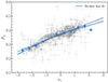 |
Fig. 12. ℱr2 as a function of x1 for SNe Ia in our cosmological sub-sample. We fit the population with a broken line (blue) and linear fit (black, dashed). We find the best-fit value of the stretch split to be at x10 = − 0.5 ± 0.2. The blue points show the data binned by stretch, taking the mean and standard error of the mean in each bin. |
where x10 is the x1 value at which the line break; this is a free parameter that is allowed to vary over the full x1 range of the sample; m1 and m2 are the slopes; and c1 and c2 are the y-intercepts before and after the line break (x10), respectively. We find a split in the population at x10 = − 0.5 ± 0.2 and the broken-line fit is also shown in Fig. 12. Using AIC as a test to compare the models, the ‘broken-line’ model is statistically preferred (difference of 52 AIC units). Interestingly, the best-fit value of the stretch split (x10 = − 0.5 ± 0.2) is consistent with what was found by Ginolin et al. (2024), x10 = −0.49 ± 0.06), where it is argued that the α term in SN Ia standardisation is non-linear, with the low stretch mode only originating from older populations and the high stretch mode containing SNe Ia from both old and young populations (Nicolas et al. 2021).
5.3. The secondary maximum in the r band for standardisation
We also tested the secondary maximum in the r band as an alternative standardisation parameter in the absence of x1, as Shariff et al. (2016) did for the secondary maximum in the J band. To this end, we used the colour-corrected Hubble residuals (not corrected for x1 or the host mass step, values adopted from Ginolin et al. 2024) and compared the correlation with x1, t2(r), and ℱr2. We find that although the correlation with t2(r) is statistically significant (> 5σ), the correlation between the Hubble residual and t2(r) is weaker than with x1, with Pearson’s correlation coefficients of r = −0.34, −0.50, respectively. On the other hand, ℱr2 shows a slightly stronger correlation with the colour-corrected Hubble residuals, with r = −0.52 at the > 5σ confidence level. The root mean square (rms) dispersion of the Hubble residuals is also reduced when using ℱr2 instead of x1 (rms = 0.220 and 0.224 mag, respectively). We perform bootstrapping to estimate the robustness of these results (Efron 1983; Efron & Tibshirani 1997). We sampled the data points with replacements from the original sample 1000 times to generate of alternative sub-samples of the same size. We computed 95 per cent confidence intervals from our bootstrapping and find −0.58 ≤ r ≤ −0.46 for the correlation between the colour-corrected Hubble residuals and ℱr2. The 95 per cent confidence interval for the correlation with x1 is −0.55 ≤ r ≤ −0.42, meaning these correlations are consistent. The correlations between the colour-corrected Hubble residuals and x1 as well as ℱr2 are shown in Fig. 13.
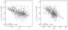 |
Fig. 13. Colour corrected Hubble residuals as a function of x1 (left) and ℱr2 (right) for the cosmological sub-sample. Pearson’s r correlation coefficients and the rms dispersion of the Hubble residuals are shown in the plots. |
Hayden et al. (2019) found that x1 measured from the rising part of the light curve showed a stronger correlation with the peak magnitude than x1 calculated from the post-peak light curve. Our results are not aligned with this and suggest that the post-peak light curve contains more information. Although it is interesting that we find ℱr2 to be a better standardisation parameter than x1, the measurement of ℱr2 relies on the presence of data at phases > 10 d, at which time the SN will have dimmed significantly compared to at maximum light. Moreover, the measurement of ℱr2 also requires data around maximum light because the peak magnitude in the r band is required to normalise the light curve to peak. Consequently, standardisation using x1 requires less data and would be preferable in most cases.
5.4. Considering which intrinsic parameters impact the secondary maximum
The timing of the secondary maximum is thought to be a temperature effect: the lower the temperature, the earlier the shift in the dominant ionisation state of the IGEs. However, the models presented by Kasen (2006) showed that the amount of stable and radioactive IGEs produced in the explosion, the distribution of IGEs throughout the ejecta, and metallicity may also affect the secondary maximum. We will use our observational data to test the impact of these parameters on the secondary maximum in the r band.
We first investigated the impact of the temperature of the ejecta on the timing of the secondary maximum by checking if there is evolution of t2(r) with the pseudo-equivalent width (pEW) of the Si II features, using the pEW values presented by Burgaz et al. (2025). Specifically, we used the pEW of the 5972 Å line as a proxy for the temperature of the ejecta. The ratio between the pEWs of the 5972 and 6355 Å lines is more commonly used as a proxy for temperature (Nugent et al. 1995; Hachinger et al. 2008), but Burgaz et al. (2025) find that the pEW of the 5972 Å line is a better tracer of peak magnitude/x1 and therefore temperature, because the 6355 Å line becomes saturated for faint SNe Ia. Our findings are in agreement, since we found a statistically significant linear trend between t2(r) and the pEW of the 5972 Å (Pearson’s correlation coefficient r = −0.38 at the > 5σ level), but no statistically significant trend between t2(r) and the ratio of the pEWS of the 5972 Å and 6355 Å lines (2.5σ). Assuming the pEW of the 5972 Å Si II line is a good proxy for temperature, this correlation indicates that t2(r) is impacted by temperature, as expected. However, the correlation is weak (Pearson’s correlation coefficient r = −0.38). This could be driven by the fact that SNe Ia with the largest t2(r) values are expected to have very weak Si II 5972 Å pEW values, and in some cases may not be measurable. At the other extreme, SNe Ia with strong Si II 5972 Å pEW values may not have a measurable secondary maximum. If both of these extremes were measurable, it could strengthen the correlation. Alternatively, there could be other factors affecting the timing of the secondary maximum, such as nickel-mixing, metallicity, or nickel mass, although we note that the nickel mass should also be strongly correlated with temperature.
To test the impact of the mass of IGEs produced and their distribution throughout the ejecta, we fit the g- and r-band light curves in our sample with the TURTLS 1D radiative transfer code, which models the early light curves of thermonuclear SNe (Magee et al. 2018, 2020). We used the same suite of 355 Mch-models as presented in Deckers et al. (2022), which contains four ejected 56Ni-masses (0.4, 0.5, 0.6, and 0.8 M⊙), five different 56Ni-distributions, two density profiles, and nine different kinetic energies of the ejecta. We follow the fitting method described in Deckers et al. (2022). In order to reliably constrain the best fitting model, the light curve needs to have good data coverage, especially at early times (Magee et al. 2020). We require the first data point to be no later than 14 d before maximum light in the g band, and a minimum cadence of 3 d. This reduces the number of light curves that we are able to fit with the TURTLS models to 499. We take the 56Ni-mass and 56Ni-distribution from the best matching TURTLS model to each SN Ia, and the 3σ confidence interval is determined by the range of model that fall within 3σ of the normalised reduced-χ2 = 1 (see Deckers et al. 2022, for further details). Similarly to the findings in Deckers et al. (2022), we find that the majority of the SN Ia light curves are fit with the two most extended nickel distributions and are not able to test for correlations with this parameter. We have been able to analyse the effect of nickel mass and find that SNe Ia with a higher estimated nickel mass tend to have a later secondary maximum at the 3.6σ level, as well as a stronger secondary maximum at the 2.5σ level, which agrees with the prediction made by Kasen (2006). We note that the nickel mass parameter in the TURTLS models measures the amount of radioactive nickel produced in the explosion, whereas the study by Kasen (2006) considered the total mass of IGE, combining radioactive and stable material.
Kasen (2006) also showed that metallicity impacts the secondary maximum, but we are unable to measure metallicity for the SNe Ia in our sample. However, Kasen (2006) predicted that as metallicity increases, the secondary maximum is pushed to earlier phases and that earlier secondary maxima should be as bright, if not brighter than later ones. Our observations of normal SNe Ia in the r band do not support this because ℱr2 shows a positive linear trend with t2(r) at a > 5σ confidence level, meaning that in our sample, later secondary maxima tend to be brighter. However, we do not find a significant positive trend between ℱi2 and t2(i). As discussed in Sect. 5.1, one interpretation of these results could be that a change in metallicity has a stronger impact on the secondary maximum in the i band than in the r band.
The models presented in Kasen (2006) predict a third bump in SN Ia light curves at around ∼80 d post maximum light in the B band, due to the recombination of singly ionised iron lines to neutral iron. Unfortunately, the ZTF DR2 light curves do not have sufficiently high S/N at these phases to confirm or reject this prediction. Moreover, Kasen (2006) stated that the LTE approximations made to produce the models are not applicable at these late epochs, and this may result in a further delay of the third maximum as well as a weakening of the bump. Kasen (2006) also predicted that the third bump should be most prominent in the J band, but the model predictions presented by (Blondin et al. 2015, Appendix C) show that the only strong Fe I features at 100 d post explosion exist in the U band; so it is unlikely that this recombination would leave any visible signature in the r/i-band photometry. However, we would encourage a future study to focus on getting high S/N data, in a range of wavelengths, at epochs between 80–150 d to search for signatures of the third maximum.
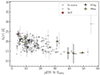 |
Fig. 14. Time of t2(r) in the r band as a function of the pEW of the 5972 Å Si II line. |
6. Conclusions
We measured the time and strength of the secondary maximum in the r band for a sample of 893 SNe Ia using GP fits. Our main results are as follows:
-
We find > 5σ correlations between Δm15(g) and the timing and strength of the secondary maximum, confirming that fainter and faster evolving SNe Ia have earlier and weaker secondary maxima, and brighter, slower evolving SNe Ia have later and stronger secondary maxima.
-
We find that sub-classes of SNe Ia which are speculated to experience interaction with a CSM/envelope (03fg- and 02es-like, as well as Ia-CSM) have higher values of ℱr2 than expected from the general trend of the sample, which can be explained by additional flux contribution from said interaction. Interestingly, we also find the 91T-like SNe Ia in general show higher ℱr2-values than the trend, which could point to these SNe Ia experiencing some interaction. Several 02cx-like SNe Ia show higher ℱr2-values which could be attributed to a bound remnant left behind after an incomplete explosion.
-
We constrained the transparency timescales for our sample, finding that the distribution peaks at 35.9 ± 0.1 d, but there is a tail to the lower transparency timescales. We fit the distribution with a bimodal Gaussian and find that the higher transparency timescale mode dominates, but there is a second component that peaks at 30.9 ± 0.4 d.
-
The lower transparency timescale component of the bimodal Gaussian, peaking at 30.9 ± 0.4 d, is produced almost exclusively by SNe Ia residing in locally red environments. The main peak at 35.9 ± 0.1 d is produced by SNe Ia in both locally red and blue environments.
-
The transparency timescales of most of the SNe Ia in our cosmological sample (97 per cent) are consistent with predictions from double detonation explosion models, whereas only 28 per cent are consistent with the predictions from delayed detonation models.
-
We measured the total ejected mass using two methods: from the transparency timescale, which was estimated from ℱr2, or from the correlation that Mej shows with x1. Both methods are derived from bolometric light curves. The distributions of Mej that we find from the two methods we applied are consistent, with medians of 1.3 ± 0.3 and 1.2 ± 0.2 M⊙, respectively.
-
We identified a spectral feature that sits in the r band around 6500 Å, which begins to strengthen during the onset of the secondary maximum. Using a NLTE radiative transfer model, we tentatively identified this feature as Fe II.
-
From the spectral time series of SN 1999by (a 91bg-like SN Ia), we find that these same features appear in the spectrum as early as 3 d post maximum, supporting the suggestion that the secondary maximum is not visible in 91bg-like SNe Ia because it coincides with the primary peak.
-
We test the ability of the secondary maximum to work as a standardisation parameter and find that ℱr2 shows a stronger correlation than x1 with the colour-corrected Hubble residuals, with Pearson’s correlation coefficients of r = −0.52 and −0.50, respectively. The rms dispersion the Hubble residuals dispersion is reduced by 0.004 mag when using ℱr2 to correct, as compared to x1.
-
We find a slight non-linearity in the correlation between x1 and ℱr2 for the cosmological sub-sample. We fit the correlation with a broken line and find a split at x10 = − 0.5 ± 0.2. Interestingly, Senzel et al. (2025) noticed a similar non-linearity between x1 and the local SN colour, and Ginolin et al. (2024) found a split in x1 at −0.49 ± 0.06 when plotted against the standardised Hubble residuals, which is consistent with our findings.
-
We find that although the timing of the secondary maximum is thought to be primarily driven by temperature, the correlation between the pEW of Si II line at 5972 Å and the timing of the secondary maximum is weak (r = −0.38).
-
We find a 3.6σ correlation between the amount of radioactive nickel produced in the explosion and the timing of the secondary maximum.
-
We conclude the metallicity is a non-dominant parameter for variations of the secondary maximum because the 5σ trend between t2(r) and ℱr2 opposes the trend expected from changes in metallicity predicted by Kasen (2006).
The large sample of SNe Ia provided by ZTF has enabled us to study the secondary maximum in the r band in great detail, both photometrically and spectroscopically. The 706 normal SNe Ia in our sample have allowed us to constrain the ranges of the parameters of the secondary maximum. Here, we present an analysis for some of peculiar SN Ia sub-classes, but future studies with greater numbers of, for instance, 91bg-like SNe Ia, will be better suited to constrain the range of when recombination occurs. The broken line fit between x1 and ℱr2, which resulted in two populations of SNe Ia split by x10 = − 0.5 ± 0.2, should be investigated in greater detail in future studies as this may hold the key to determining if there are two main progenitor scenarios, resulting in slightly differing SN Ia properties. We re-iterate the importance of ℱr2 because it can be measured for any SN Ia sub-class regardless of light curve morphology. Although in most cases it is easier to constrain x1 than ℱr2, it is interesting to note that ℱr2 is better able to standardise SN Ia light curves. Standardisation using ℱr2 may be useful for specific cases during LSST, where a SN Ia might have insufficient data on the rise to constrain x1, but does have sufficient data later on, which would allow for constraints to be placed on the peak in the r band and ℱr2.
Data availability
The properties of the secondary maximum derived from our Gaussian Process fits are available at the CDS via anonymous ftp to cdsarc.cds.unistra.fr (130.79.128.5) or via https://cdsarc.cds.unistra.fr/viz-bin/cat/J/A+A/694/A12.
In this paper we refer to the secondary shoulder in the r band, t2(r), as a secondary maximum, even if dF/dt = 0 does not exist in the light curve.
The models presented in Gronow et al. (2021) extend the range of core and He shell masses and were produced to explain the variations seen in the bolometric magnitudes of SNe Ia.
Acknowledgments
MD, KM, GD, UB, and JHT are funded by the EU H2020 ERC grant no. 758638. LJS acknowledge support by the European Research Council (ERC) under the European Union’s Horizon 2020 research and innovation program (ERC Advanced Grant KILONOVA No. 885281). LJS acknowledges support by Deutsche Forschungsgemeinschaft (DFG, German Research Foundation) – Project-ID 279384907 – SFB 1245 and MA 4248/3-1. L.G. acknowledges financial support from the Spanish Ministerio de Ciencia e Innovación (MCIN) and the Agencia Estatal de Investigación (AEI) 10.13039/501100011033 under the PID2020-115253GA-I00 HOSTFLOWS project, from Centro Superior de Investigaciones Científicas (CSIC) under the PIE project 20215AT016 and the program Unidad de Excelencia María de Maeztu CEX2020-001058-M, and from the Departament de Recerca i Universitats de la Generalitat de Catalunya through the 2021-SGR-01270 grant. This work has been supported by the research project grant “Understanding the Dynamic Universe” funded by the Knut and Alice Wallenberg Foundation under Dnr KAW 2018.0067. This project has received funding from the European Research Council (ERC) under the European Union’s Horizon 2020 research and innovation program (grant agreement n 759194 – USNAC). AG acknowledges support from Vetenskapsrådet, the Swedish Research Council, project 2020-03444. SD acknowledges support from the Marie Curie Individual Fellowship under grant ID 890695 and a Junior Research Fellowship at Lucy Cavendish College. LH is funded by the Irish Research Council under grant number GOIPG/2020/1387. T.E.M.B. acknowledges financial support from the Spanish Ministerio de Ciencia e Innovación (MCIN), the Agencia Estatal de Investigación (AEI) 10.13039/501100011033, and the European Union Next Generation EU/PRTR funds under the 2021 Juan de la Cierva program FJC2021-047124-I and the PID2020-115253GA-I00 HOSTFLOWS project, from Centro Superior de Investigaciones Científicas (CSIC) under the PIE project 20215AT016, and the program Unidad de Excelencia María de Maeztu CEX2020-001058-M. Y.-L.K. has received funding from the Science and Technology Facilities Council [grant number ST/V000713/1]. Based on observations obtained with the Samuel Oschin Telescope 48-inch and the 60-inch Telescope at the Palomar Observatory as part of the Zwicky Transient Facility project. ZTF is supported by the National Science Foundation under Grants No. AST-1440341 and AST-2034437 and a collaboration including partners Caltech, IPAC, the Weizmann Institute of Science, the Oskar Klein Center at Stockholm University, the University of Maryland, Deutsches Elektronen-Synchrotron and Humboldt University, the TANGO Consortium of Taiwan, the University of Wisconsin at Milwaukee, Trinity College Dublin, Lawrence Livermore National Laboratories, IN2P3, University of Warwick, Ruhr University Bochum, Northwestern University and former partners the University of Washington, Los Alamos National Laboratories, and Lawrence Berkeley National Laboratories. Operations are conducted by COO, IPAC, and UW. SED Machine is based upon work supported by the National Science Foundation under Grant No. 1106171. The ZTF forced-photometry service was funded under the Heising-Simons Foundation grant #12540303 (PI: Graham). This work made use of the Heidelberg Supernova Model Archive (HESMA), https://hesma.h-its.org.
References
- Amenouche, M., Rosnet, P., Smith, M., et al. 2025, A&A, 694, A3 (ZTF DR2 SI) [NASA ADS] [CrossRef] [EDP Sciences] [Google Scholar]
- Arnett, W. D. 1982, ApJ, 253, 785 [Google Scholar]
- Ashall, C., Lu, J., Burns, C., et al. 2020, ApJ, 895, L3 [NASA ADS] [CrossRef] [Google Scholar]
- Barbary, K., Bailey, S., Barentsen, G., et al. 2022, https://doi.org/10.5281/zenodo.6363879 [Google Scholar]
- Bellm, E. C., Kulkarni, S. R., Barlow, T., et al. 2019, PASP, 131, 068003 [Google Scholar]
- Blagorodnova, N., Neill, J. D., Walters, R., et al. 2018, PASP, 130, 035003 [Google Scholar]
- Blondin, S., Dessart, L., & Hillier, D. J. 2015, MNRAS, 448, 2766 [NASA ADS] [CrossRef] [Google Scholar]
- Blondin, S., Dessart, L., Hillier, D. J., & Khokhlov, A. M. 2017, MNRAS, 470, 157 [Google Scholar]
- Boone, K. 2019, AJ, 158, 257 [NASA ADS] [CrossRef] [Google Scholar]
- Burgaz, U., Maguire, K., Dimitriadis, G., et al. 2025, A&A, 694, A9 (ZTF DR2 SI) [NASA ADS] [CrossRef] [EDP Sciences] [Google Scholar]
- Burke, J., Howell, D. A., Sarbadhicary, S. K., et al. 2021, ApJ, 919, 142 [NASA ADS] [CrossRef] [Google Scholar]
- Burnham, K. P., & Anderson, D. R. 2004, Sociol. Methods Res., 33, 261 [Google Scholar]
- Burns, C. R., Stritzinger, M., Phillips, M. M., et al. 2014, ApJ, 789, 32 [Google Scholar]
- Burns, C. R., Parent, E., Phillips, M. M., et al. 2018, ApJ, 869, 56 [Google Scholar]
- Contreras, C., Hamuy, M., Phillips, M. M., et al. 2010, AJ, 139, 519 [Google Scholar]
- Deckers, M., Maguire, K., Magee, M. R., et al. 2022, MNRAS, 512, 1317 [NASA ADS] [CrossRef] [Google Scholar]
- Deckers, M., Graur, O., Maguire, K., et al. 2023, MNRAS, 521, 4414 [NASA ADS] [CrossRef] [Google Scholar]
- Dekany, R., Smith, R. M., Riddle, R., et al. 2020, ApJ, 132, 1009 [Google Scholar]
- Dhawan, S., Leibundgut, B., Spyromilio, J., & Maguire, K. 2015, MNRAS, 448, 1345 [NASA ADS] [CrossRef] [Google Scholar]
- Dhawan, S., Leibundgut, B., Spyromilio, J., & Blondin, S. 2016, A&A, 588, 84 [Google Scholar]
- Dhawan, S., Leibundgut, B., Spyromilio, J., & Blondin, S. 2017, A&A, 602, A118 [NASA ADS] [CrossRef] [EDP Sciences] [Google Scholar]
- Dhawan, S., Bulla, M., Goobar, A., et al. 2018, MNRAS, 480, 1445 [NASA ADS] [CrossRef] [Google Scholar]
- Dimitriadis, G., Foley, R. J., Arendse, N., et al. 2021, ApJ, 927, 78 [Google Scholar]
- Dimitriadis, G., Maguire, K., Karambelkar, V. R., et al. 2023, MNRAS, 521, 1162 [NASA ADS] [CrossRef] [Google Scholar]
- Dimitriadis, G., Burgaz, U., Deckers, M., et al. 2025, A&A, 694, A10 (ZTF DR2 SI) [NASA ADS] [CrossRef] [EDP Sciences] [Google Scholar]
- Duvenaud, D. K. 2014, Ph.D. Thesis, University of Cambridge, UK [Google Scholar]
- Efron, B. 1983, J. Am. Stat. Assoc., 78, 316 [CrossRef] [Google Scholar]
- Efron, B., & Tibshirani, R. 1997, J. Am. Stat. Assoc., 92, 548 [Google Scholar]
- Elias, J. H., Frogel, J. A., Hackwell, J. A., & Persson, S. E. 1981, ApJ, 251, L13 [NASA ADS] [CrossRef] [Google Scholar]
- Fink, M. 2010, Ph.D. Thesis, Technical University of Munich, Germany [Google Scholar]
- Fink, M., Röpke, F. K., Hillebrandt, W., et al. 2010, A&A, 514, A53 [NASA ADS] [CrossRef] [EDP Sciences] [Google Scholar]
- Galbany, L., Ashall, C., Hoeflich, P., et al. 2019, A&A, 630, A76 [NASA ADS] [CrossRef] [EDP Sciences] [Google Scholar]
- Ginolin, M., Rigault, M., Smith, M., et al. 2024, A&A, submitted [arXiv: 2405.20965] (ZTF DR2 SI) [Google Scholar]
- González-Gaitán, S., Gaitán, G., Hsiao, E. Y., et al. 2014, ApJ, 795, 142 [CrossRef] [Google Scholar]
- Graham, M. J., Kulkarni, S. R., Bellm, E. C., et al. 2019, PASP, 131, 078001 [Google Scholar]
- Graur, O. 2023, MNRAS, 530, 4950 [Google Scholar]
- Graur, O., Gonzalez, E. P., Burke, J., et al. 2023, MNRAS, 526, 2977 [NASA ADS] [CrossRef] [Google Scholar]
- Gronow, S., Collins, C., Ohlmann, S. T., et al. 2020, A&A, 635, A169 [NASA ADS] [CrossRef] [EDP Sciences] [Google Scholar]
- Gronow, S., Collins, C. E., Sim, S. A., & Roepke, F. K. 2021, A&A, 649, A155 [NASA ADS] [CrossRef] [EDP Sciences] [Google Scholar]
- Guy, J., Astier, P., Baumont, S., et al. 2007, A&A, 466, 11 [NASA ADS] [CrossRef] [EDP Sciences] [Google Scholar]
- Hachinger, S., Mazzali, P. A., Tanaka, M., et al. 2008, MNRAS, 389, 1087 [NASA ADS] [CrossRef] [Google Scholar]
- Hamuy, M., Phillips, M. M., Suntzeff, N. B., et al. 1996, AJ, 112, 2438 [NASA ADS] [CrossRef] [Google Scholar]
- Harvey, L., Maguire, K., Magee, M. R., et al. 2023, MNRAS, 522, 4444 [NASA ADS] [CrossRef] [Google Scholar]
- Hayden, B., Rubin, D., & Strovink, M. 2019, ApJ, 871, 219 [NASA ADS] [CrossRef] [Google Scholar]
- Hicken, M., Challis, P., Jha, S., et al. 2009, ApJ, 700, 331 [Google Scholar]
- Hillebrandt, W., Kromer, M., Röpke, F. K., & Ruiter, A. J. 2013, Front. Phys., 8, 116 [Google Scholar]
- Hoeflich, P. 2017, Handbook of Supernovae (Springer), 1151 [CrossRef] [Google Scholar]
- Hoflich, P., & Khokhlov, A. 1996, ApJ, 457, 500 [CrossRef] [Google Scholar]
- Hoeflich, P., Gerardy, C. L., Fesen, R. A., & Sakai, S. 2002, ApJ, 568, 791 [NASA ADS] [CrossRef] [Google Scholar]
- Hoogendam, W. B., Ashall, C., Galbany, L., et al. 2022, ApJ, 928, 103 [NASA ADS] [CrossRef] [Google Scholar]
- Hoogendam, W. B., Shappee, B. J., Brown, P. J., et al. 2023, ApJ, 966, 139 [Google Scholar]
- Hsiao, E. Y., Conley, A., Howell, D. A., et al. 2007, ApJ, 663, 1187 [Google Scholar]
- Jack, D., Hauschildt, P. H., & Baron, E. 2011, A&A, 528, A141 [NASA ADS] [CrossRef] [EDP Sciences] [Google Scholar]
- Jack, D., Baron, E., & Hauschildt, P. H. 2015, MNRAS, 449, 3581 [NASA ADS] [CrossRef] [Google Scholar]
- Jeffery, D. J. 1999, ArXiv e-prints [arXiv:astro-ph/9907015] [Google Scholar]
- Jha, S. W. 2017, Handbook of Supernovae (Springer), 375 [CrossRef] [Google Scholar]
- Jha, S. W., Maguire, K., & Sullivan, M. 2019, Nat. Astron., 3, 706 [NASA ADS] [CrossRef] [Google Scholar]
- Johansson, J., Smith, M., Rigault, M., et al. 2025, A&A, in prep. (ZTF DR2 SI) [Google Scholar]
- Kasen, D. 2006, ApJ, 649, 939 [NASA ADS] [CrossRef] [Google Scholar]
- Kasen, D., & Woosley, S. E. 2007, ApJ, 656, 661 [NASA ADS] [CrossRef] [Google Scholar]
- Kenworthy, W. D., Jones, D. O., Dai, M., et al. 2021, ApJ, 923, 265 [NASA ADS] [CrossRef] [Google Scholar]
- Kim, Y. L., Rigault, M., Neill, J. D., et al. 2022, PASP, 134, 024505 [NASA ADS] [CrossRef] [Google Scholar]
- Krisciunas, K., Phillips, M. M., Stubbs, C., et al. 2001, AJ, 122, 1616 [NASA ADS] [CrossRef] [Google Scholar]
- Kromer, M., Sim, S. A., Fink, M., et al. 2010, ApJ, 719, 1067 [Google Scholar]
- Kromer, M., Fink, M., Stanishev, V., et al. 2013a, MNRAS, 429, 2287 [NASA ADS] [CrossRef] [Google Scholar]
- Kromer, M., Pakmor, R., Taubenberger, S., et al. 2013b, ApJ, 778, L18 [NASA ADS] [CrossRef] [Google Scholar]
- Kromer, M., Fremling, C., Pakmor, R., et al. 2016, MNRAS, 459, 4428 [NASA ADS] [CrossRef] [Google Scholar]
- Kromer, M., Ohlmann, S., Röpke, F. K., et al. 2017, MmSAI, 88, 312 [NASA ADS] [Google Scholar]
- Lach, F., Callan, F. P., Sim, S. A., & Röpke, F. K. 2022, A&A, 659, A27 [NASA ADS] [CrossRef] [EDP Sciences] [Google Scholar]
- Leloudas, G., Hsiao, E. Y., Johansson, J., et al. 2015, A&A, 574, A61 [NASA ADS] [CrossRef] [EDP Sciences] [Google Scholar]
- Li, Z., Zhang, T., Wang, X., et al. 2022, ApJ, 927, 142 [NASA ADS] [CrossRef] [Google Scholar]
- Liu, Z., Roepke, F. K., & Han, Z. 2023, Res. A&A, 23, 082001 [Google Scholar]
- Lu, J., Ashall, C., Hsiao, E. Y., et al. 2021, ApJ, 920, 107 [NASA ADS] [CrossRef] [Google Scholar]
- Magee, M. R., Sim, S. A., Kotak, R., & Kerzendorf, W. E. 2018, A&A, 614, 1 [Google Scholar]
- Magee, M. R., Maguire, K., Kotak, R., et al. 2020, A&A, 634, A37 [NASA ADS] [CrossRef] [EDP Sciences] [Google Scholar]
- Maoz, D., Mannucci, F., & Nelemans, G. 2014, ARA&A, 52, 107 [Google Scholar]
- Masci, F. J., Laher, R. R., Rusholme, B., et al. 2019, PASP, 131, 018003 [Google Scholar]
- Matheson, T., Kirshner, R. P., Challis, P., et al. 2008, AJ, 135, 1598 [CrossRef] [Google Scholar]
- Mazzali, P. A., Nomoto, K., Cappellaro, E., et al. 2001, ApJ, 547, 988 [NASA ADS] [CrossRef] [Google Scholar]
- Miller, A. A., Magee, M. R., Polin, A., et al. 2020, ApJ, 898, 56 [NASA ADS] [CrossRef] [Google Scholar]
- Müller-Bravo, T. E., Sullivan, M., Smith, M., et al. 2022, MNRAS, 512, 3266 [CrossRef] [Google Scholar]
- Nicolas, N., Rigault, M., Copin, Y., et al. 2021, A&A, 649, A74 [NASA ADS] [CrossRef] [EDP Sciences] [Google Scholar]
- Nobili, S., Amanullah, R., Garavini, G., et al. 2005, A&A, 437, 789 [NASA ADS] [CrossRef] [EDP Sciences] [Google Scholar]
- Nomoto, K., Thielemann, F.-K., & Yokoi, K. 1984, ApJ, 286, 644 [NASA ADS] [CrossRef] [Google Scholar]
- Nugent, P., Phillips, M., Baron, E., Branch, D., & Hauschildt, P. 1995, ApJ, 455, L147 [NASA ADS] [CrossRef] [Google Scholar]
- Ohlmann, S. T., Kromer, M., Fink, M., et al. 2014, A&A, 572, A57 [NASA ADS] [CrossRef] [EDP Sciences] [Google Scholar]
- Pakmor, R., Kromer, M., Roepke, F. K., et al. 2010, Nature, 463, 61 [NASA ADS] [CrossRef] [Google Scholar]
- Pakmor, R., Kromer, M., Taubenberger, S., et al. 2012, ApJ, 747, 10 [NASA ADS] [CrossRef] [Google Scholar]
- Papadogiannakis, S., Dhawan, S., Morosin, R., & Goobar, A. 2019a, MNRAS, 485, 2343 [NASA ADS] [CrossRef] [Google Scholar]
- Papadogiannakis, S., Goobar, A., Amanullah, R., et al. 2019b, MNRAS, 483, 5045 [Google Scholar]
- Perlmutter, S., Turner, M. S., & White, M. 1999, Phys. Rev. Lett., 83, 670 [CrossRef] [Google Scholar]
- Pessi, P. J., Folatelli, G., Anderson, J. P., et al. 2019, MNRAS, 488, 4239 [NASA ADS] [CrossRef] [Google Scholar]
- Pessi, P. J., Hsiao, E. Y., Folatelli, G., et al. 2021, MNRAS, 510, 4929 [Google Scholar]
- Phillips, M. M. 1993, ApJ, 413, L105 [Google Scholar]
- Pinto, P. A., & Eastman, R. G. 2000, ApJ, 530, 757 [NASA ADS] [CrossRef] [Google Scholar]
- Pskovskii, I. P. 1977, Sov. Astron., 21, 675 [NASA ADS] [Google Scholar]
- Rasmussen, C. E., & Williams, C. K. I. 2006, Gaussian Processes for Machine Learning, 248 [Google Scholar]
- Rau, A., Kulkarni, S. R., Law, N. M., et al. 2009, PASP, 121, 1334 [NASA ADS] [CrossRef] [Google Scholar]
- Riess, A. G., Filippenko, A. V., Challis, P., et al. 1998, AJ, 116, 1009 [Google Scholar]
- Rigault, M., Neill, J. D., Blagorodnova, N., et al. 2019, A&A, 627, A115 [NASA ADS] [CrossRef] [EDP Sciences] [Google Scholar]
- Rigault, M., Smith, M., Goobar, A., et al. 2025, A&A, 694, A1 (ZTF DR2 SI) [NASA ADS] [CrossRef] [EDP Sciences] [Google Scholar]
- Ruiter, A. J. 2020, IAUS, 357, 1 [NASA ADS] [Google Scholar]
- Scalzo, R., Aldering, G., Antilogus, P., et al. 2014, MNRAS, 440, 1498 [NASA ADS] [CrossRef] [Google Scholar]
- Scolnic, D. M., Jones, D. O., Rest, A., et al. 2018, ApJ, 859, 28 [NASA ADS] [CrossRef] [Google Scholar]
- Seitenzahl, I. R., Ciaraldi-Schoolmann, F., Röpke, F. K., et al. 2013, MNRAS, 429, 1156 [NASA ADS] [CrossRef] [Google Scholar]
- Seitenzahl, I. R., Kromer, M., Ohlmann, S. T., et al. 2016, A&A, 592, 57 [Google Scholar]
- Senzel, R., Maguire, K., Burgaz, U., et al. 2025, A&A, 694, A14 (ZTF DR2 SI) [NASA ADS] [CrossRef] [EDP Sciences] [Google Scholar]
- Shariff, H., Dhawan, S., Jiao, X., et al. 2016, MNRAS, 463, 4311 [NASA ADS] [CrossRef] [Google Scholar]
- Sharma, Y., Sollerman, J., Fremling, C., et al. 2023, ApJ, 948, 52 [NASA ADS] [CrossRef] [Google Scholar]
- Shingles, L. J., Sim, S. A., Kromer, M., et al. 2020, MNRAS, 492, 2029 [NASA ADS] [CrossRef] [Google Scholar]
- Shingles, L. J., Flörs, A., Sim, S. A., et al. 2022, MNRAS, 512, 6150 [NASA ADS] [CrossRef] [Google Scholar]
- Siebert, M. R., Dimitriadis, G., Polin, A., & Foley, R. J. 2020, ApJ, 900, 15 [NASA ADS] [CrossRef] [Google Scholar]
- Sim, S. A., Röpke, F. K., Kromer, M., et al. 2013, IAUS, 281, 267 [NASA ADS] [Google Scholar]
- Smith, M., Rigault, M., et al. 2025, A&A, in prep. (ZTF DR2 SI) [Google Scholar]
- Stritzinger, M., Leibundgut, B., Walch, S., & Contardo, G. 2006a, A&A, 450, 241 [NASA ADS] [CrossRef] [EDP Sciences] [Google Scholar]
- Stritzinger, M., Mazzali, P. A., Sollerman, J., & Benetti, S. 2006b, A&A, 460, 793 [NASA ADS] [CrossRef] [EDP Sciences] [Google Scholar]
- Taubenberger, S. 2017, Handbook of Supernovae (Springer), 317 [CrossRef] [Google Scholar]
- Taubenberger, S., Hachinger, S., Pignata, G., et al. 2008, MNRAS, 385, 75 [NASA ADS] [CrossRef] [Google Scholar]
- Taubenberger, S., Benetti, S., Childress, M., et al. 2011, MNRAS, 412, 2735 [NASA ADS] [CrossRef] [Google Scholar]
- Taubenberger, S., Kromer, M., Hachinger, S., et al. 2013, MNRAS, 432, 3117 [NASA ADS] [CrossRef] [Google Scholar]
- Taubenberger, S., Floers, A., Vogl, C., et al. 2019, MNRAS, 488, 5473 [NASA ADS] [Google Scholar]
- Taylor, G., Lidman, C., Tucker, B. E., et al. 2021, MNRAS, 504, 4111 [NASA ADS] [CrossRef] [Google Scholar]
- Tripp, R. 1998, A&A, 331, 815 [NASA ADS] [Google Scholar]
- Turatto, M., Benetti, S., Cappellaro, E., et al. 1996, MNRAS, 283, 1 [NASA ADS] [CrossRef] [Google Scholar]
All Tables
All Figures
|
Fig. 1. Example of GP fit to a r-band light curve (top). The GP fit is shown as a red and the 1σ uncertainty is shown as the red shaded region. The area over which the integrated flux under the secondary maximum, ℱr2, is calculated is indicated by the grey shaded region, and t2(r) by the black dashed. The first derivative of the GP light curve (middle). This light curve has a secondary shoulder rather than a secondary maximum because the first derivative is not equal to zero. The second derivative of the GP light curve (bottom), shows that the time of the onset of the secondary maximum is the time at which the second derivative is equal to zero, also known as an inflection point. |
| In the text | |
|
Fig. 2. Impact of various kernel and length scale choices on a GP fit of a ZTF SN Ia light curve. If the uncertainties in the data are underestimated, not including a white noise kernel will result in unrealistic wiggles in an attempt to fit all the points (top left). Even if the uncertainties are not underestimated in the data, a lack of a white noise kernel can result in an underestimation of the uncertainty of the GP fit, as is visible between 10–30 d in the light curve shown in the top-right panel. With limited data at the edge of the fitting regions, not including a constant kernel can result in deviating behaviour at the edge regions (bottom left). We optimise the length scale during the fit in the bottom-right panel, which in this case resulted in ℓ = 12.3 d. By setting a length scale, the likelihood is higher to either over-fit if the length scale is too short (ℓ = 3 d), or to under-fit and miss important features if the length scale is too long (ℓ = 30 d). The ideal value for the length scale will depend on the cadence of the data, which varies across our sample. |
| In the text | |
|
Fig. 3. Distribution of t2(r) for the 63 SNe Ia with a detected true bump (i.e. dF/dt = 0 exists), measured either as the local maximum (dF/dt = 0, x-axis) or the inflection point (d2F/dt2 = 0, y-axis). We systematically find a lower t2(r) if measured as the point of inflection versus the local maximum in the light curve. |
| In the text | |
|
Fig. 4. Impact of K-corrections on t2(r) (top) and ℱr2 (bottom), as a function of redshift and x1 (left) and c (right). The colour of the data points represents the residual between the measured parameter in the SALT3 model at that point and the same model at z = 0. Overall, the impact of K-corrections is small, with a maximum residual on ℱr2 of 0.014 and on t2(r) of 0.66 d. |
| In the text | |
|
Fig. 5. Averaged spectra between 0–10, 10–20, 20–30, 30–40, and 40–50 d in the r- and i-band wavelength ranges. The phases are relative to g-band maximum. Spectra are binned into −3 ≤ x1 < 0 (dashed) and 0 ≤ x1 < 3 (solid). The grey shaded regions indicate the spectral regions where a feature appears during the onset of the secondary maximum. The numbers in the brackets represent the number of spectra going into each bin (first number represents the number of spectra in the −3 ≤ x1 < 0 bin, and the second number are the number of spectra in the 0 ≤ x1 < 3 bin). We also show the filter response functions of the ZTF r and i bands in black. In the bottom panel we show a spectral timeseries of SN 1999by (a 91bg-like SN Ia). |
| In the text | |
|
Fig. 6. Timing of secondary maximum (t2(x), top) and normalised integrated flux in the range of 15–40 d (ℱx2, bottom) in the r band (left) and i band (right) as a function of Δm15(g) for our sample. We also show simple linear regression fits to the whole sample (black dashed lines). We find a non-zero slope at the > 5σ confidence level for t2(r), t2(i), ℱr2, but not for ℱi2 with Δm15(g). |
| In the text | |
|
Fig. 7. Histogram showing the distribution of ℱr2 for the ZTF DR2 sample with the flux integral divided by 25 d (shaded orange) or divided by 20 d (dashed orange), compared to the distribution found for PTF and iPTF by Papadogiannakis et al. (2019a) (black). The median of the PTF+iPTF population is 1.5σ higher than the median of the ZTF DR2 population when the integral is divided by 25 d, but the ZTF distribution is consistent with the PTF+iPTF distribution if the integral is divided by 20 d instead. |
| In the text | |
|
Fig. 8. t2(r) vs. t2(i). We also show a simple linear regression fit (black dashed line) through the full data set.t2(r) vs. t2(i). We also show a simple linear regression fit (black dashed line) through the full data set. |
| In the text | |
|
Fig. 9. Spectra showing the breakdown of species contributing to each feature from a NLTE radiative transfer model of the W7 explosion model at 30 d (top), 40 d (middle), and 50 d (bottom) past explosion. |
| In the text | |
|
Fig. 10. Distributions of transparency timescales for the whole cosmological sub-sample are shown at the top (grey), along with a bimodal Gaussian fit (solid grey line) and its individual components (dashed grey). The arrows show the ranges of transparency timescales predicted by doubledet_2010 (Fink et al. 2010; Kromer et al. 2010), doubledet_2020, (Gronow et al. 2020), doubledet_2021(Gronow et al. 2021), ddt_2010 (Fink 2010), ddt_2013 (Seitenzahl et al. 2013; Sim et al. 2013), ddt_2014 (Ohlmann et al. 2014), SCH, PDDEL, and DDC (Blondin et al. 2017) explosions models. In the bottom plot we separate the transparency timescale distribution into SNe Ia with blue local colours ((g − z)local ≤ 1.0, blue) or red local colours ((g − z)local > 1.0, red). We show bimodal Gaussian the fits to both distributions, and the individual components making up the fit are shown as dotted lines. The Akaike Information Criterion (AIC) test prefers a bimodal fit for the SNe Ia in red local environments, but it does not show a preference for either the double component fit or single component fit for the SNe Ia population in blue environments, so we also show the single component fit as a dashed line to this population. |
| In the text | |
|
Fig. 11. Comparison between the total ejected mass derived from |
| In the text | |
|
Fig. 12. ℱr2 as a function of x1 for SNe Ia in our cosmological sub-sample. We fit the population with a broken line (blue) and linear fit (black, dashed). We find the best-fit value of the stretch split to be at x10 = − 0.5 ± 0.2. The blue points show the data binned by stretch, taking the mean and standard error of the mean in each bin. |
| In the text | |
|
Fig. 13. Colour corrected Hubble residuals as a function of x1 (left) and ℱr2 (right) for the cosmological sub-sample. Pearson’s r correlation coefficients and the rms dispersion of the Hubble residuals are shown in the plots. |
| In the text | |
|
Fig. 14. Time of t2(r) in the r band as a function of the pEW of the 5972 Å Si II line. |
| In the text | |
Current usage metrics show cumulative count of Article Views (full-text article views including HTML views, PDF and ePub downloads, according to the available data) and Abstracts Views on Vision4Press platform.
Data correspond to usage on the plateform after 2015. The current usage metrics is available 48-96 hours after online publication and is updated daily on week days.
Initial download of the metrics may take a while.