| Issue |
A&A
Volume 694, February 2025
|
|
|---|---|---|
| Article Number | A107 | |
| Number of page(s) | 16 | |
| Section | Cosmology (including clusters of galaxies) | |
| DOI | https://doi.org/10.1051/0004-6361/202347386 | |
| Published online | 10 February 2025 | |
Spherical bias in the 3D reconstruction of the ICM density profile in galaxy clusters
1
INAF – Istituto di Astrofisica Spaziale e Fisica Cosmica di Milano, Via A. Corti 12, 20133 Milano, Italy
2
INAF – Osservatorio Astronomico di Trieste, Via Tiepolo 11, I-34131 Trieste, Italy
3
IFPU – Institute for Fundamental Physics of the Universe, Via Beirut 2, 34151 Trieste, Italy
4
INAF – Osservatorio Astronomico di Brera, Via E. Bianchi 46, 23807 Merate (LC), Italy
5
DiSAT, Università degli Studi dell’Insubria, Via Valleggio 11, I-22100 Como, Italy
6
Dipartimento di Fisica, Universitá degli Studi di Milano, Via G. Celoria 16, 20133 Milano, Italy
⋆ Corresponding author; This email address is being protected from spambots. You need JavaScript enabled to view it.
Received:
6
July
2023
Accepted:
7
September
2024
Abstract
Context. X-ray observations of galaxy clusters are routinely used to derive radial distributions of intracluster medium (ICM) thermodynamical properties, such as density and temperature. However, observations only allow access to quantities projected on the celestial sphere, so an assumption on the three-dimensional distribution of the ICM is necessary. Usually, spherical geometry is assumed.
Aims. The aim of this paper is to determine the bias due to this approximation on the reconstruction of the ICM density radial profile of a cluster sample and on the intrinsic scatter of the density profiles’ distribution, particularly when the substructures of clusters are not masked.
Methods. We used simulated clusters for which we can access the three-dimensional ICM distribution. In particular, we considered a sample of 98 simulated clusters drawn from THE THREE HUNDRED project. For each cluster, we simulated 40 different observations by projecting the cluster along 40 different lines of sight. We extracted the ICM density profile from each observation, assuming the ICM to be spherically distributed. For each line of sight, we then considered the mean density profile over the sample and compared it with the three-dimensional density profile given by the simulations. We thus derived the spherical bias in the density profile by considering the ratio between the observed and the input quantities. We also studied the bias in the intrinsic scatter of the density profile distribution by performing the same procedure.
Results. We find a bias in the density profile, bn, smaller than 10% for R ≲ R500, and it increases up to ≈50% for larger radii. The bias in the intrinsic scatter profile, bs, is higher, reaching a value of ≈100% for R ≈ R500. We find that the bias for both of the analyzed quantities strongly depends on the morphology composition of the objects in the sample. For clusters that do not show large-scale substructures, both bn and bs are reduced by a factor of two. Conversely, for systems that do show large-scale substructures, both bn and bs increase significantly.
Key words: galaxies: clusters: general / galaxies: clusters: intracluster medium / X-rays: galaxies / X-rays: galaxies: clusters
© The Authors 2025
 Open Access article, published by EDP Sciences, under the terms of the Creative Commons Attribution License (https://creativecommons.org/licenses/by/4.0), which permits unrestricted use, distribution, and reproduction in any medium, provided the original work is properly cited.
This article is published in open access under the Subscribe to Open model. This email address is being protected from spambots. You need JavaScript enabled to view it. to support open access publication.
1. Introduction
Galaxy clusters play a crucial role in the understanding of both astrophysical processes and large-scale structure evolution. They are the largest virialized objects generated from small density fluctuations in the primordial era and grew hierarchically under their own gravity influence. Indeed, galaxy clusters trace the evolution of the Universe and its composition, so important cosmological knowledge can be derived by studying their properties (e.g., Voit 2005; Allen et al. 2011). Moreover, many astrophysical processes take place within galaxy clusters, and the baryonic component properties derived from cluster studies are used for astrophysics and fundamental physics studies (e.g., Arnaud 2005; Tozzi & Norman 2001). In this context, X-ray observations play a major role, as they can detect the emission associated with the intracluster medium (ICM), which is the hot and rarefied plasma that lies among the galaxies. This component contributes ∼15% to the total cluster matter and represents the main baryonic component, as stars and galaxies make up only a few percent. In particular, X-ray observations enable ICM density and temperature profiles to be derived. These are crucial quantities for obtaining cluster properties since they provide the starting point for mass measurements. In particular, they are used to derive the total cluster mass through the hydrostatic equilibrium equation. Moreover, the ICM density profile is used to obtain the gas mass, which is a widely used proxy of the total mass of clusters (Arnaud et al. 2010; Kravtsov et al. 2006; Pratt et al. 2019), and to measure the cluster mass function and hence the mass density, Ωm, which is a fundamental quantity for cosmological studies. Therefore, the reconstruction of the ICM density profile assumes a significant role in cosmological studies. Moreover, in the era of precision astronomy and cosmology (Allen et al. 2011; Planck Collaboration XX 2014; Salvati et al. 2018), it is very important to be aware of the contribution of each systematic error source that can affect any measure and to quantify them.
Every astronomical observation carries an intrinsic aspect that could introduce systematic errors. In fact, observations can be informative only about projected quantities, so an assumption on the underlying geometry is necessary to recover three-dimensional properties, such as density profiles. In this context, the property of cluster shape also assumes a crucial role.
It is well known that the mass distribution within galaxy clusters is generally not spherical, even though determining its three-dimensional shape is still an issue. Several studies have investigated the problem using multi-wavelength techniques, such as through a combination of gravitational lensing, X-ray, and Sunyaev-Zel’dovich effect observations, both on individual clusters and cluster samples, and these studies have found a quite general triaxial morphology (Sereno et al. 2006, 2017, and references therein). However, some clusters appear more spherical and present smoother density profiles thanks to virialization processes, while others can present density inhomogeneities that make the cluster shape more intricate.
However, it is a standard practice to assume spherical geometry when deriving cluster gas properties from X-ray observations. In fact, this makes the gas distribution deprojection process easier to implement and more computationally efficient. Moreover, it is widely assumed that any possible geometrical bias in single systems is averaged out when considering cluster samples, thanks to the triaxial orientations that are assumed to be randomly distributed. Systematic errors in the gas distribution reconstruction due to spherical assumption have been investigated throughout the years, typically by comparing different deprojection models applied to different theoretical morphologies (see, e.g., Binney & Strimpel 1978; Piffaretti et al. 2003). The most recent work in the context of X-ray and Sunyaev–Zel’dovich observations is by Buote & Humphrey (2012a,b). The authors investigate the spherical averaging of galaxy clusters shaped using different ellipsoidal models. They quantify the orientation-average bias and scatter for many observables and find generally small mean biases with substantial scatter for different view orientations. However, the studies in this area of research mostly investigate the impact of elliptical shapes instead of spherical ones, considering clusters with smooth density profiles and leaving the presence of inhomogeneities aside. In the present work, we investigate the bias due to the spherical assumption on the reconstruction of the ICM density profile while considering the presence of inhomogeneities in substructures. In fact, in contrast to the cited works based on theoretical geometrical models, here we consider clusters that are simulated in a cosmological context such that their shapes are not theoretically defined following a geometrical model but are given by the cosmological framework and the gravitational interaction with the environment. For each simulated cluster, we emulated an X-ray observation on the sky plane and considered numerous different lines of sight. By using standard X-ray analysis procedures, we extracted the ICM density profile from each projected cluster, assuming spherical geometry, and compared it with the true density profile given by the simulations. In this way, we are able to quantify the bias introduced by the spherical assumption.
This paper is organized as follows: In Sect. 2, we describe the composition of the simulated cluster sample and the procedure to produce mock X-ray maps. In Sect. 3, we discuss the mock maps analysis procedure, while in Sect. 4 we present the main results of the analysis. In Sect. 5, we discuss the results, and in Sect. 6 we summarize the biases that arise from the spherical approximation in the gas density profile.
We adopted a flat Λ cold dark matter cosmology with Ωm(0) = 0.3, ΩΛ(0) = 0.7, and H0 = 70 km Mpc−1 s−1. We note that the cosmological density values are those of the simulated sample, which is characterized by a slightly lower Hubble constant (H0, sim = 67.77 km Mpc−1 s−1). However, this difference does not affect the results of this paper.
2. Dataset and production of mock maps
2.1. Dataset
This work relies on simulated galaxy clusters drawn from THE THREE HUNDRED project (Cui et al. 2018). This project comprises 324 regions re-simulated with full-physics hydro-dynamical codes selected from the dark matter only MultiDark Planck 2 simulations (Klypin et al. 2016). The aim of this work is to statistically characterize the bias introduced when deriving the ICM radial density profile of clusters and assuming a spherical geometry. This is tested on a sample that needs to be as representative as possible of the underlying cluster population and is able to reproduce the variety of morphologies. Therefore, we selected 98 clusters from THE THREE HUNDRED catalog with masses in the range 2.0 × 10¹⁴ M⊙ < M5001 < 14.3 × 10¹⁴ M⊙ (Fig. 1). The sample was built to include about 20 to 25 objects in each of the following mass intervals: [2 − 4], [4 − 6], [6 − 8], [8 − 10]×1014 M⊙, in addition to nine objects with M500 > 1015 M⊙. The selection was done by making sure that various morphologies were represented, as shown in Fig. 2. In the figure, several clusters show substructures that appear as luminous regions distinguishable from the central halo, while others have an almost spherical distribution. These features make the sample suitable to study the effects introduced by the spherical approximation, which is ordinarily used for X-ray analysis, and to quantify the related bias in the density profile reconstruction. All the clusters are fixed at redshift z = 0.3 since we are not interested in studying any possible effect due to spatial resolution. The physical properties of each cluster are reported in Table A.1.
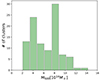 |
Fig. 1. Mass distribution of the sample of simulated clusters used in this work. The minimum and maximum values of the mass are 2.0 × 10¹⁴ M⊙ and 14.3 × 10¹⁴ M⊙, respectively. |
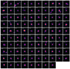 |
Fig. 2. Image gallery of the 98 galaxy clusters in the simulated sample. Each image covers an area of 5R500 × 5R500 and represents the spatial distribution of the ICM projected along one random direction in units of cm−6 Mpc. The solid circle indicates R500, while the dashed one indicates 2R500. In many clusters one or more substructures are present. The names of the simulated clusters are reported in each panel. The first number identifies the simulated region where the halo is extracted, and the second is the mass-rank index of the halo in that specific region. For example, CL0005_1 is the most massive cluster found in the fifth region. |
2.2. Simulating mock X-ray maps
The starting point of this work involved the creation of mock observations of the simulated clusters. This was done by projecting them on the sky plane and reproducing X-ray telescope effects in order to obtain an X-ray-like image.
2.2.1. Projection on the sky plane
Since telescopes observe projected objects on the sky plane, we first projected each three-dimensional simulated cluster. We created emission-measure maps from each simulated cluster with the program Smac (see Dolag et al. 2005; Ansarifard et al. 2020). The maps are centered at the position of the maximum of the density field, which coincides with our definition of the theoretical center. The field of view has a side equal to 6R500 divided into 1200 pixels, leading to a resolution of 5% R500 per pixel. This distance of 6R500 is also the length of the integration along the line of sight. By reaching such a high distance from the cluster center (3R500 ≈ 2R200 in the front and the back of the object), we were sure to include any possible large-scale structure whose emission can be visualized in the projected maps. Starting from a map oriented as the z axis of the simulation box and thus randomly oriented with respect to the cluster’s major axis, we then created other maps obtained by rotating the object with equi-spaced angles, as visually represented in Fig. 3. In this way we generated 40 emission measure (EM) maps for each simulated cluster. The chosen 40 lines of sight allowed us to uniformly investigate the object from different directions.
 |
Fig. 3. Representation on a sphere (left) and on a polar plane (right) of the forty directions along which a three-dimensional simulated cluster is projected. The directions are distributed at intervals of Δθ = 1/10 π and Δϕ = 1/8 π, with θ ∈ [0, 9/10 π] and ϕ ∈ [0, 3/8 π], where ϕ = 0 identifies the equatorial plane. Every direction is identified as (t, p), where t ∈ [0, 9] and p ∈ [0, 3] represent θ and ϕ. |
The maps were produced by summing over the contribution of all gas particles with temperature, Ti, larger than 0.3 keV and density, ρi, below the star-forming density threshold. This condition allowed for the study of the diffuse gas that emits in the considered X-ray bands. We note that the same gas particle exclusion was applied to all the quantities extracted from the simulated clusters, such as the 3D gas density profiles. To create the maps, we specifically summed the product (mi × ρi) of the selected particles once this contribution was weighted by a spline kernel with a width equal to the gas particle smoothing length.
The resulting maps are in units of a mass density squared integrated over a volume, that is [g2 cm−6 kpc2 cm]. However, the EM standard units are [cm−6 Mpc], so we needed to convert them by taking into account the proton mass, the molecular weight μ, and the electron-to-proton fraction f since the EM is referred to as the electron emission. We used the same gas parameters that characterize the simulated gas, namely μ = 0.59 and f = 1.08.
2.2.2. Generating mock maps
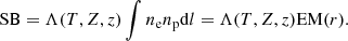
Once the 40 EM maps had been generated for each cluster, we generated mock X-ray observations. X-ray telescopes collect the incoming photons in their camera pixels, so they return counts maps. To create these maps from the EM maps, we first converted them into surface brightness (SB) maps. The EM and SB are related through the cooling function Λ(T, Z, z), which depends on the cluster temperature T, the cluster abundance Z, and the cluster redshift z:
 (1)
(1)
In the soft X-ray band, the cooling function Λ(T, Z, z) shows little dependence on either temperature or cluster abundance Z (Ettori 2000; Bartalucci et al. 2017). To ensure this fact, we computed the cooling function for different temperatures and abundances, with typical cluster temperature values that can fluctuate by 20% (Rossetti et al. 2024, cf. Fig. 11) and typical cluster abundance values that can fluctuate by 25% (Ghizzardi et al. 2021, cf. Figs. 5 and 11); Λ(T, Z) varies less than 3%. Therefore the cooling function was computed using a constant temperature and constant abundance, within the [0.5, 2.0] keV energy band. The temperature for each cluster was given by the simulations, while the metal abundance was fixed to the average value 0.25 Z⊙, as derived from (Ghizzardi et al. 2021, cf. Modified analysis of Table 1). The redshift was fixed for all clusters to z = 0.3. The cooling function was computed via XSPEC (Arnaud 1996) using the phabs (photoelectric absorbed)2 Astrophysical Plasma Emission code (APEC)3 model (Smith et al. 2001) and convolved with the telescope effective area. For our scope, we considered the XMM-Newton PN camera.
Once we generated the surface brightness maps, we converted them into X-ray-like counts maps, following the same method described in Bartalucci et al. (2023), which we briefly report here. First, we converted the surface brightness into photon counts by multiplying the surface brightness maps by the pixel surface and by an observation time of 30 ks, a typical XMM-Newton exposure time. For simplicity, we did not consider Point Spread Function and vignetting effects or the presence of malfunctioning pixels or gaps. For these reasons the exposure time is the same for all the map pixels. We then added the sky background component. We considered a mean value bkgmean = 5.165 × 10⁻³ cts arcmin−2 s−1 measured by the PN camera in the [0.5 − 2] keV band (Bartalucci et al. 2023), and we introduced spatial variations by dividing the field of view into square tiles of ∼2.35 arcmin size where the background value varies by approximately 3% (Ghirardini et al. 2018) around bkgmean. Finally, we applied a Poisson randomization to each pixel of the map to emulate the discretized photon counts. All the used parameters are reported in Table 1. The outcome of this procedure is represented in Fig. 4. Through this approach, we created 40 mock X-ray maps – one for each projection line – for each of the 98 simulated clusters.
Parameters used in the phabs/APEC model for mock map production and analysis.
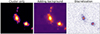 |
Fig. 4. Mock map generation process. Left panel: Map of the cluster emission. Central panel: Map of the cluster emission with the addition of the tiled background. Right panel: Map resulting from the discretization of the cluster+background map through a Poisson randomization. All maps are in units of counts. |
3. Data analysis
The main purpose of the following analysis is to determine the bias in the cluster gas density profile reconstruction due to the spherical symmetry approximation. In particular, we evaluated the effect caused by the presence of inhomogeneity in substructures. To reach this goal, we used the mock X-ray maps obtained as described in Sect. 2.2.2 to extract the gas density profiles following the same procedure used for real observations, where spherical symmetry is assumed. However, it is important to highlight a key difference between the density profile extraction procedure followed in this work and the one used in real cluster analysis. In fact, in the latter case, if any substructure appears in the observation frame, it is masked in such a way that its contribution to the cluster main emission will not be considered. Therefore, it is interesting to study how the density profile is reconstructed even with the contribution of substructures while maintaining a spherical model. Furthermore, when we have to deal with real cluster observations, it can occur that substructures are indistinguishable from the central core because of resolution issues and because they are located along the observer-core line of sight. For these reasons, it is important to evaluate the impact of the substructures on the gas density profile when it is reconstructed with a spherical shape.
3.1. Analysis of mock maps
To extract the gas density profile from every mock X-ray map, we used pyproffit4 (Eckert et al. 2016, 2020), a Python package largely used for X-ray cluster analysis in which the spherical symmetry is assumed. For each map, pyproffit first extracts the SB profile (count rate per surface and time unit), by computing the mean surface brightness in concentric annular bins and dividing by the exposure time. We extracted the SB profile up to 3R500 in annular bins of 5 arcsec width. We then converted the SB profile into an EM profile through Eq. (1). The conversion factor Λ(T, Z, z) was computed via XPSEC with the same procedure and parameters used for the production of the mock maps (see Sect. 2.2.2 and Table 1).
The obtained EM profile was then deprojected to obtain the electron density profile. In fact, the EM is defined as the projection along the line of sight of the gas density:
 (2)
(2)
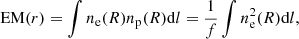
where f is the electron-to-proton fraction. The EM profile deprojection process to obtain the electron density profile was performed by pyproffit while assuming a spherical geometry. That is, the EM profile was modeled as a combination of β-models:
![Mathematical equation: $$ \begin{aligned} \mathrm{EM}(r) = \sum _i A_i \phi _i (r) = \sum _i A_i \Big [1+\Big (\frac{r}{r_{c,i}}\Big )^2\Big ]^{-3\beta _i + \frac{1}{2}}\cdot \end{aligned} $$](/articles/aa/full_html/2025/02/aa47386-23/aa47386-23-eq3.gif) (3)
(3)
In particular, we modeled the EM profile by combining six β-models. Such a spherical geometry is widely used since the β-model functions ϕi can be analytically deprojected, thus returning the deprojected functions Φi(R) = ∫ϕi(r)dl. The combination of the deprojected functions Φi gives the following electron density profile:
![Mathematical equation: $$ \begin{aligned} n_{\rm e}(R) = \sum _i C_i \Phi _i(R) = \sum _i C_i \Big [1+\left(\frac{R}{r_{c,i}}\right)^2\Big ]^{-3\beta _i}. \end{aligned} $$](/articles/aa/full_html/2025/02/aa47386-23/aa47386-23-eq4.gif) (4)
(4)
The parameters of the β-models (βi, rc, i, Ai) in Eq. (3) were inferred by pyproffit from the observed EM profile by maximizing a Poissonian likelihood. The background was considered a flat surface brightness profile described by a single parameter. In particular, we considered the radial range [2.5, 3]R500 as the background fitting region, where the background emission dominates over the cluster emission. The deprojection result is the electron density profile of the cluster (Eq. (4)). The procedure is schematized in Fig. 5.
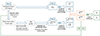 |
Fig. 5. Schematic representation of the procedure described in Sects. 2.2.2 and 3 to derive the gas density bias and the intrinsic scatter due to the spherical assumption. |
3.2. Analysis of density profiles
In this section we study how the spherical symmetry assumption impacts the cluster gas density profile reconstruction. In particular, we study how the presence of substructures influences the deprojection process.
The spherical assumption’s impact can be derived by comparing the extracted profiles with the input profiles, that is, the density profiles given directly by simulations. The input profiles are obtained by computing the density on spherical shells starting from the cluster center5. We divided the analysis by first studying each cluster individually and then the sample as a whole.
3.2.1. Single cluster analysis
As a first step of the analysis, we considered each cluster individually so that we could compare the profiles extracted along each line ( ) of sight with the input density profile (
 ) and study how well it is reconstructed by considering the ratio between each extracted profile and the input one. This type of analysis shows how the spherical approximation works on specific clusters, allowing us to understand how substructures and their projected position (which depends on the line of sight) modify the reconstructed profile.
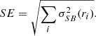
3.2.2. Sample analysis
For the main part of the analysis, we considered the entire sample observed only from one line of sight at a time instead of considering every cluster from different lines of sight. This approach reproduces what a real observer would actually see. We were able to access at least 40 different realizations of the same sample (one for each projection line) and compared the results, giving us the opportunity to study how different projections impact the density profile reconstruction. To perform this type of analysis, we defined the sample global electron density profile ne and the related intrinsic scatter σintr. These quantities were defined as follows. The global density profile is the logarithmic average profile of the 98 cluster profiles ne, cl in the sample. Assuming that their distribution is log-normal, the logarithmic average is then defined as the expected value of the logarithmic distribution of the 98 density profiles:
![Mathematical equation: $$ \begin{aligned} n_{\rm e} = \exp {\Big [\xi + \frac{\sigma ^2}{2}\Big ]}, \end{aligned} $$](/articles/aa/full_html/2025/02/aa47386-23/aa47386-23-eq7.gif) (5)
(5)
where ξ and σ are respectively the mean and the standard deviation of the normal distribution of log ne, cl. The intrinsic scatter σintr represents the physical dispersion of the sample profiles around the global profile ne, and it is related to the total dispersion σ as
 (6)
(6)
where σstat is the statistical error computed as the square root of counts within each radial bin.
For each sample realization, we computed the observed global density profile  and the observed intrinsic scatter
  . We then compared different sample realizations and considered the mean observed global profile
  of the normal distribution of all the observed global profiles
  . The same procedure was performed on the intrinsic scatter to obtain the mean observed intrinsic scatter
  of all the observed intrinsic scatter
  . We also defined the respective input quantities, that is, the mean input global density profile
  and the mean input intrinsic scatter
  .
.
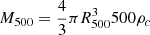
By comparing the observed and input quantities, we could determine the biases on the density and scatter profiles, respectively bn and bs, associated with the spherical geometry assumption. We defined the bias bq for the quantity q as
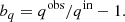 (7)
(7)
4. Results
4.1. Single cluster results
The results of the analysis outlined in Sect. 3.2.1 on single clusters show the impact of cluster morphology on the density profile reconstruction. We report two illustrative and opposite cases: one “regular” cluster (i.e., without substructures) and one “irregular” cluster (i.e., with substructures). These cases are shown in the X-ray-like maps reported in Fig. 6.
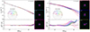 |
Fig. 6. Gas density profile along 40 lines of sight for two clusters chosen as examples. In the left figure, the regular cluster CL0129_1 is reported, while the right figure presents the irregular cluster CL0005_1. For both figures, the black line refers to the input gas density profile, and the colored lines refer to the observed profiles, extracted assuming spherical geometry for the gas spatial distribution. Each color refers to a specific line of sight, as reported on the polar plane. In the bottom panel of both figures, the observed-to-input ratio is reported for each line of sight. It is evident how the input profile is better reconstructed for the regular cluster. On the right of each figure, three cluster projections are reported (the color of the edges identifies the corresponding line of sight). The solid and the dashed circles refer respectively to R500 and 2R500. We note the smooth shape of CL0129_1, regardless of the projection, and the irregular shape of CL0005_1, where the substructure position changes with the projection. |
In the first case, we show the cluster CL0129_1 (Fig. 6, left). It does not present any substructure, as shown in the three reported maps, and it exhibits a spherical core. The cluster indeed appears similar to itself regardless of the considered projection. Therefore, the 40 density profiles should appear similar to each other. Moreover, each reconstructed profile reproduces the input one quite well. The ratio between the extracted and the input profiles is ≲1.1 for a very large radial range (R ≲ 1.5R500). This result indicates that the assumed spherical symmetry does not introduce any relevant bias when studying clusters with few substructures.
In the second case, we show the irregular cluster CL0005_1 (Fig. 6, right). It features an evident substructure visible in all the three cluster projections. Its presence can significantly modify the apparent shape of the cluster that an observer would see. For example, an observer along the line of sight (9,2; the red line of sight in Fig. 6) might consider this cluster as a regular one (with no substructures in the outer regions), whereas along the (2,1) projection (the green line of sight), the substructure is clearly distinguishable from the central core. Because of this, the reconstructed density profiles are expected to differ from one line of sight to another, as actually shown by the results and indeed from the input profile. The shape of the reconstructed profile is affected by the substructure position. If one considers once again the projection along (9,2), one can see that the corresponding reconstructed density profile shows a “bump” at small radii, where the substructure is seen. In this region, the observed profile results are overestimated with respect to the input one. If we instead consider the (2,1) projection (green), we can see that the bump in the density profile shape is located at larger radii, where the substructure appears. More generally, for each line of sight, the reconstructed profile overestimates the input profile where the substructure appears. This overestimation can be partially due to a projection effect and partially due to the spherical modeling process (both contribute to it), making the substructure deprojected density higher than the real three-dimensional one (see Appendix B). From these considerations, we inferred that for irregular clusters the spherical approximation introduces an overall overestimation of the extracted profile with respect to the input one in the region where the substructures appear, with typical ratios 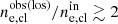 for R ≳ R500.
4.2. Sample results
The results of the analysis outlined in Sect. 3.2.2 of each sample realization are reported in Fig. 7. In the left panel of the figure, we report the bias 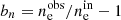 on the global density profile, while in right panel we report the intrinsic scatter σintr profile and the associated bias
  . For both of these quantities, we report the 40 results on each sample realization (qobs(los)) and also the mean over all the projections (qobs).
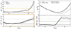 |
Fig. 7. Characterization of the bias introduced by the spherical assumption for the whole sample. Left figure: Bias in ICM density profile due to spherical assumption. In the bottom panel, we report the zoom of the innermost region. The gray lines refer to the global density profile for each sample realization (one for each line of sight), the solid black line refers to the mean over the sample realizations, and the dash-dotted lines refer to the 1σ value. Right figure: Scatter profile of the sample’s density profiles around the global density profile (upper panel) and the relative bias due to the spherical assumption (bottom panel). The lighter black lines refer to the scatter profile for each sample realization, the solid black line to the mean over the sample realizations, and the dash-dotted lines to the 1σ value. The black dashed line refers to the input profile, and the green dashed line refers to the 50% level. |
The bias in the global density profile due to the spherical approximation shows a very similar behavior regardless of the line of sight, exhibiting an overall overestimation of the reconstructed profile that gradually increases with the radius. More specifically, in the innermost regions for R ≲ R500, the mean bias introduced by the spherical approximation is ≲10% and decreases down to ≲5% for R ≲ 0.4R500. Conversely, the bias increases in the outer regions, reaching 50% at R ∼ 2R500 (see Table 2). As expected, this behavior does not significantly differ from one sample realization to another; that is, the line of sight does not introduce significant differences in the bias.
Results of the analysis for the biases on the global density profile and on the intrinsic scatter of a cluster population.
These results show that the reconstructed global density profile is generally overestimated. We can hypothesize that this is due to the presence of irregular clusters in the sample since, as we observed in Sect. 4.1, the presence of substructures causes an overestimation of the observed cluster emission and thus of the observed density profile in the region where the substructure appears. Therefore, if several irregular clusters are included in the sample, the global density profile should be overestimated over a large radial range, as shown by the results. Moreover, the bias increases with the radius. This can be due to the substructure’s apparent position: The profile tends to be more overestimated if the substructure appears in the outer regions (see Appendix B).
Next, we move on to the analysis of the results on the sample intrinsic scatter profile. First of all, we note that the observed total dispersion σ (see Eq. (6)) almost entirely coincides with the intrinsic scatter σintr, as the statistical scatter σstat is very small because we used mock observations with high statistics derived from simulations. With these results in hand, we observed that the intrinsic scatter (Fig. 7, right upper panel) behavior is similar for both the observed and the input scatter profiles: They show a convex shape with a minimum in 0.4 − 0.8R500. At smaller radii, the scatter increases since simulated clusters present different core densities and slopes. In the outer regions, the scatter increases since clusters more frequently show substructures in these regions.
The difference between the observed and the input scatter can be evaluated by analyzing the bias bs (Fig. 7, right lower panel). We observed that the observed and input scatter mostly differ in the outer regions. For R < 0.3R500, the difference between the observed and input scatter is in fact not very significant, with an associated bias bs < 10%. This is due to the fact that in these regions the observed density profile closely follows its corresponding input profile (bn ≲ 5% for R ≲ 0.4R500) regardless of the cluster and the line of sight so that the distribution of the observed profiles is very similar to the distribution of the input ones, and thus the bias in the scatter is small. Conversely, in the outer regions the observed scatter increases much more than the input scatter, with an associated bias bs ≳ 100% for R > 0.6R500. This is likely due to substructures that show up at different projected radii along different lines of sight, impacting a large radial range.
For both the global density and the intrinsic scatter profiles, we hypothesized that the differences between the observed and the input quantities could mainly be due to the presence of substructures in some clusters. This hypothesis can be tested and verified by dividing the sample into subsamples with different morphological compositions.
5. Substructures impact analysis
We tested the impact of substructures by defining two subsamples that we labeled as the “regular sample” and the “irregular sample”, which were respectively composed of clusters presenting or free from substructure emission. Thanks to this differentiation, we could isolate the substructures’ impact and evaluate the related bias.
5.1. Definition of subsamples
To divide the sample into regular and irregular clusters, we defined a “shape estimator” (SE), that is, a quantity that can evaluate the presence of substructures. Substructures modify the SB profile shape by introducing an SB peak where the substructure appears (for an example, see Fig. B.1). Obviously, the peak position depends on the considered projection. We took advantage of the large number of projections we had, and for each cluster we compared the SB profiles from different lines of sight. Clusters that present substructures show different SB profile shapes depending on the considered projection, while regular clusters show very similar profiles regardless of the line of sight (Fig. 8). Therefore, we could distinguish between regular and irregular clusters by evaluating the SB profile distribution width, normalized for the mean surface brightness value (i.e., their scatter σSB).
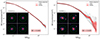 |
Fig. 8. Comparison between each projected SB profile distribution of a regular (left panel) and irregular (right panel) cluster. The regular cluster maps appear very similar to each other despite the projection, so all the SB profiles that refer to different lines of sight present a similar behavior as well and thus show a narrow distribution. On the other hand, the irregular cluster appears very different depending on the considered projection, so its SB profile presents different shapes, making the profile distribution scatter considerable (depending on the radius). |
There are several morphological indicators that are used in the literature to classify clusters that have been calibrated on X-ray observations (e.g., see Campitiello et al. 2022 for a recent work using these indicators). However, their application to our sample of simulated X-ray observations would require further calibrations that are beyond the scope of this work. For this reason, we defined the SE as the combination of different profiles’ distribution scatters at different radii:
 (8)
(8)
In particular, we considered seven radii between 0.1R500 and 2.0R500 (see Appendix C). We then computed the SE for all the clusters in the sample and ordered them in ascending order with respect to the SE value so that the first clusters are the most regular ones, while the last are the most irregular. We identified two subsamples, one of regular and one of irregular clusters, by respectively selecting the first and the last 15 SE-ordered clusters (see Fig. C.2).
The regular clusters are characterized by a lack of substructures. However, their morphologies typically differ from a spherical shape, showing triaxial structures. Thanks to this characteristic, we could use the regular sample to study the spherical assumption bias in nonspherical objects without substructures (i.e., without the main source of deviation from the spherical symmetry).
5.2. Analysis of subsamples
We repeated the same analysis outlined in Sect. 3.2.2 on the two subsamples defined in the previous section, obtaining for each subsample 40 global density profiles  and 40 global scatter profiles
  (one for each sample realization along a line of sight) and the mean global density and scatter profiles over the 40 sample realizations,
  and
and  . The results are reported in Fig. 9 and Table 2 and are compared with the results obtained in Sect. 4.2 for the complete sample. As one can see, the sample composition strongly affects both the reconstructed density and scatter profiles.
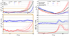 |
Fig. 9. Same as Fig. 7 but for the regular and irregular subsamples. Left figure: Bias in ICM density profile due to the spherical assumption. In the bottom panel, the zoom of the innermost region is reported. Right figure: Scatter profile of each sample’s density profiles around the global density profile (upper panel) and the relative bias due to the spherical assumption (bottom panel). The black lines refer to the complete sample, the red lines to the irregular sample, and the blue lines to the regular sample. The lighter lines refer to the global density profile for each sample realization (one for each line of sight), the solid lines to the mean over the sample realizations, and the dash-dotted lines to a 1σ value. In the right figure, the dashed lines refer to the input profile; the green dashed line refers to the 50% level. |
For what concerns the density profile, we observed that for the regular cluster sample, the observed profile differs from the input profile by less than 10% up to a very large radial range (R ≈ 1.5R500), while for the complete sample, the 10%-bias range is achieved only up to R ≈ 0.9R500. In addition, for the regular sample, the bias remains ≲5% for a very extended radial range (R ≲ 1.2R500). On the other hand, for the irregular cluster sample, the observed density profile is well reconstructed (bn < 10%) for a smaller radial range (R < 0.7R500), while at R ≈ R500, the observed profile is overestimated by more than 20% with respect to the input profile.
We can conclude that the differences between the observed and the input profiles strongly depend on the sample composition and, in particular, on its large-scale morphology. That is, if the sample is composed of clusters that present substructures, then the density profile of the sample is less accurately reconstructed than for regular cluster samples. This is highlighted also by the radius at which the difference between the reconstructed and the input profile can be seen. For irregular clusters, the bias increases significantly at R ≈ R500, where indeed substructures begin to appear. Considering the complete sample, where both regular and irregular clusters are present, the substructure effects are reduced by the regular clusters so that the global profile of the sample is better reconstructed for a large radial range than the case where only irregular clusters are considered.
Differences between the regular and irregular samples became even more pronounced when we investigated the scatter. The regular sample presents an observed scatter much more similar to the input one than the complete sample, with bs ≲ 10% for R ≲ 0.5R500. The bias reaches a maximum value of ≈90% for 0.6R500 ≲ R ≲ 0.7R500 and then stabilizes to ≈50% for R > R500. For the irregular sample, we could see that the observed scatter differs from the input one much more than the complete and the regular samples, even for small radii, being ≲10% only for R ≲ 0.2R500, while at R ≈ 0.3R500 we find bs ≈ 40%. The bias increases up to very high values in the outer regions. We found a maximum bias of ≈400% for 0.7R500 ≲ R ≲ R500 and bs ≈ 200% for R > R500.
These results confirm that the observed density profiles of irregular cluster results are overestimated in the radial range where the substructures appear. Since the position of the substructure differs from one cluster to another, the sample profile distribution will be broader than the input one. For a regular cluster, this is obviously not valid. Since there are no substructures, the density profile is well reconstructed for all the clusters in the sample, making the sample profile distribution much more similar to the input one.
The impact of the substructures is also noticeable when studying the results for different sample realizations. For the regular sample, every line of sight shows a very similar behavior, while in the irregular sample important differences can be found from one sample realization to another. This is obviously due to substructures. In the regular sample, each cluster appears similar to itself regardless of the line of sight, so there are no large differences between the sample realizations. On the other hand, in the irregular sample, each cluster can appear in very different shapes depending on the considered line of sight, thus creating very different sample realizations (see Fig. C.3).
These results led us to the conclusion that the high bias measured for the complete sample is indeed due to substructures. In fact, since the sample is composed of both regular and irregular clusters, the profile distribution is primarily enlarged by irregular clusters.
6. Conclusions
In this paper, we tested the three-dimensional reconstruction of the global ICM density profile of a cluster population and its intrinsic scatter profile when spherical geometry is assumed. We used a sample composed of 98 simulated galaxy clusters that was built to be representative of a common cluster population. We considered 40 different sample realizations by projecting each cluster along 40 different lines of sight. For each sample realization, we emulated an X-ray observation of all the clusters in the sample, and we extracted the electron density profile while assuming a spherical geometry for the gas spatial distribution. We then derived the global gas density profile for each sample realization and compared it with the input global density profile, which was directly given by the simulations. We were therefore able to determine the bias introduced by the spherical assumption in the reconstruction of the ICM density profile. We also analyzed the bias in the intrinsic scatter of the profile distribution for each sample realization.
For the global density profile, we found the following:
-
It is well reconstructed for a large radial range, with a bias due to the spherical approximation smaller than 10% for R ≲ R500.
-
In the innermost regions (R ≲ 0.4R500), the bias decreases down to values ≲5%.
-
At large radii (R > R500), the bias increases up to ≈50% because of the impact of substructures.
-
The bias strongly depends on the sample composition. If the sample is composed of regular clusters (without overdensity substructures), the bias is smaller (bn ≲ 20% for R ≲ 2R500 and bn < 5% for R ≲ 1.5R500). However, if it is only composed of clusters that show substructures, the bias increases considerably (bn > 10% for R ≳ 0.7R500).
For the intrinsic scatter of the density profiles’ distribution, we found the following:
-
The mean reconstructed scatter follows the input scatter quite well in the inner regions, with a bias bs < 10% for R ≲ 0.3R500.
-
In the outer regions, the reconstructed scatter results are considerably higher than the input one, with an associated bias that rapidly increases up to ≈100% in 0.4R500 ≲ R ≲ 0.7R500, maintaining this value for larger radii. This is due to substructures in the outer regions of some clusters in the sample that cause the density profile to be overestimated in the radial range where substructures appear, making the sample profile distribution broader. Similar to the bias in the density profile, the bias in the scatter strongly depends on the sample composition: If we consider a sample composed exclusively of clusters that do not show substructures, the bias in the profile distribution scatter is bs < 10% for a larger radial range (R ≲ 0.5R500), and in the outer regions, it is reduced by a factor of two, down to ≈50%. If we consider a sample composed exclusively of clusters that do show substructures, the bias is ≲10% only for R ≲ 0.2R500 (at R ≈ 0.3R500 we find bs ≈ 40%). In the outer regions, it increases up to a maximum value of ≈400% for 0.7R500 ≲ R ≲ R500 and bs ≈ 200% for R > R500.
The analysis outlined in this paper led to the estimation of the biases that should be considered when 3D reconstruction of the ICM density profile through spherical approximation is performed on real observations, particularly when considering cluster substructures. In fact, even if the substructures are generally masked out from real observations, it can occur that some of them appear indistinguishable from the central core and consequently cannot be masked, introducing the bias that we evaluate in this work. Moreover, the shape of the intrinsic scatter found in the analysis can be used as a comparison for real observations of cluster samples.
 , with ρc critical density at cluster redshift.
We stress that fact the profiles computed using spherical shells cannot be used to study the triaxial geometry of the cluster.
Acknowledgments
We acknowledge financial contribution from the contracts ASI-INAF Athena 2019-27-HH.0, “Attività di Studio per la comunità scientifica di Astrofisica delle Alte Energie e Fisica Astroparticellare” (Accordo Attuativo ASI-INAF n. 2017-14-H.0), and from the European Union’s Horizon 2020 Programme under the AHEAD2020 project (grant agreement n. 871158). This work has been made possible by the ‘The Three Hundred’ collaboration, which received financial support from the European Union’s Horizon 2020 Research and Innovation programme under the Marie Sklodowskaw-Curie grant agreement number 734374, i.e. the LACEGAL project. The simulations used in this paper have been performed in the MareNostrum Supercomputer at the Barcelona Supercomputing centre, thanks to CPU time granted by the Red Española de Supercomputación.
References
- Allen, S. W., Evrard, A. E., & Mantz, A. B. 2011, ARA&A, 49, 409 [Google Scholar]
- Ansarifard, S., Rasia, E., Biffi, V., et al. 2020, A&A, 634, A113 [NASA ADS] [CrossRef] [EDP Sciences] [Google Scholar]
- Arnaud, K. A. 1996, in Astronomical Data Analysis Software and Systems V, eds. G. H. Jacoby, & J. Barnes, ASP Conf. Ser., 101, 17 [NASA ADS] [Google Scholar]
- Arnaud, M. 2005, in Background Microwave Radiation and Intracluster Cosmology, eds. F. Melchiorri, & Y. Rephaeli, 77 [Google Scholar]
- Arnaud, M., Pratt, G. W., Piffaretti, R., et al. 2010, A&A, 517, A92 [CrossRef] [EDP Sciences] [Google Scholar]
- Bartalucci, I., Arnaud, M., Pratt, G. W., et al. 2017, A&A, 608, A88 [NASA ADS] [CrossRef] [EDP Sciences] [Google Scholar]
- Bartalucci, I., Molendi, S., Rasia, E., et al. 2023, A&A, 674, A179 [NASA ADS] [CrossRef] [EDP Sciences] [Google Scholar]
- Binney, J., & Strimpel, O. 1978, MNRAS, 185, 473 [NASA ADS] [CrossRef] [Google Scholar]
- Buote, D. A., & Humphrey, P. J. 2012a, MNRAS, 420, 1693 [CrossRef] [Google Scholar]
- Buote, D. A., & Humphrey, P. J. 2012b, MNRAS, 421, 1399 [NASA ADS] [CrossRef] [Google Scholar]
- Campitiello, M. G., Ettori, S., Lovisari, L., et al. 2022, A&A, 665, A117 [NASA ADS] [CrossRef] [EDP Sciences] [Google Scholar]
- Cui, W., Knebe, A., Yepes, G., et al. 2018, MNRAS, 480, 2898 [Google Scholar]
- Dolag, K., Hansen, F. K., Roncarelli, M., & Moscardini, L. 2005, MNRAS, 363, 29 [Google Scholar]
- Eckert, D., Roncarelli, M., Ettori, S., et al. 2015, MNRAS, 447, 2198 [Google Scholar]
- Eckert, D., Ettori, S., Coupon, J., et al. 2016, A&A, 592, A12 [NASA ADS] [CrossRef] [EDP Sciences] [Google Scholar]
- Eckert, D., Finoguenov, A., Ghirardini, V., et al. 2020, Open J. Astrophys., 3, 12 [NASA ADS] [CrossRef] [Google Scholar]
- Ettori, S. 2000, MNRAS, 311, 313 [NASA ADS] [CrossRef] [Google Scholar]
- Ghirardini, V., Ettori, S., Eckert, D., et al. 2018, A&A, 614, A7 [NASA ADS] [CrossRef] [EDP Sciences] [Google Scholar]
- Ghizzardi, S., Molendi, S., van der Burg, R., et al. 2021, A&A, 646, A92 [NASA ADS] [CrossRef] [EDP Sciences] [Google Scholar]
- Kalberla, P. M. W., Burton, W. B., Hartmann, D., et al. 2005, A&A, 440, 775 [NASA ADS] [CrossRef] [EDP Sciences] [Google Scholar]
- Klypin, A., Yepes, G., Gottlöber, S., Prada, F., & Heß, S. 2016, MNRAS, 457, 4340 [Google Scholar]
- Kravtsov, A. V., Vikhlinin, A., & Nagai, D. 2006, ApJ, 650, 128 [Google Scholar]
- Nagai, D., & Lau, E. T. 2011, ApJ, 731, L10 [NASA ADS] [CrossRef] [Google Scholar]
- Piffaretti, R., Jetzer, P., & Schindler, S. 2003, A&A, 398, 41 [NASA ADS] [CrossRef] [EDP Sciences] [Google Scholar]
- Planck Collaboration XX. 2014, A&A, 571, A20 [NASA ADS] [CrossRef] [EDP Sciences] [Google Scholar]
- Pratt, G. W., Arnaud, M., Biviano, A., et al. 2019, Space Sci. Rev., 215, 25 [Google Scholar]
- Roncarelli, M., Ettori, S., Borgani, S., et al. 2013, MNRAS, 432, 3030 [NASA ADS] [CrossRef] [Google Scholar]
- Rossetti, M., Eckert, D., Gastaldello, F., et al. 2024, A&A, 686, A68 [NASA ADS] [CrossRef] [EDP Sciences] [Google Scholar]
- Salvati, L., Douspis, M., & Aghanim, N. 2018, A&A, 614, A13 [NASA ADS] [CrossRef] [EDP Sciences] [Google Scholar]
- Sereno, M., De Filippis, E., Longo, G., & Bautz, M. W. 2006, ApJ, 645, 170 [NASA ADS] [CrossRef] [Google Scholar]
- Sereno, M., Ettori, S., Meneghetti, M., et al. 2017, MNRAS, 467, 3801 [NASA ADS] [CrossRef] [Google Scholar]
- Smith, R. K., Brickhouse, N. S., Liedahl, D. A., & Raymond, J. C. 2001, ApJ, 556, L91 [Google Scholar]
- Tozzi, P., & Norman, C. 2001, ApJ, 546, 63 [NASA ADS] [CrossRef] [Google Scholar]
- Voit, G. M. 2005, Rev. Mod. Phys., 77, 207 [Google Scholar]
Appendix A: Sample properties
Table of the sample properties.
Appendix B: Substructures impact
In our study the observed density profiles result generally overestimated with respect to the input profile. In particular, the overestimation arise in the region where the substructure appears. This result can be justified considering two effects: the projection effect and the model effect.
The density profile derives in fact from the measured surface brightness profile. The observed surface brightness profile is obtained by measuring the projected gas emission averaged on annular bins, so that the three-dimensional emission is redistributed on circular shells instead of spherical shells. Since surface brightness is related to square density as SB ∝ ⟨n2⟩, if inhomogeneities are present in the gas distribution their emission is enhanced. This can cause an overestimation of the gas density profile in the order of  where C = ⟨n2⟩/⟨n⟩2 is the clumpiness factor (see e.g. Nagai & Lau 2011; Roncarelli et al. 2013; Eckert et al. 2015). These effects make substructures appear as high emission peak.
Moreover, the model we used does not take into account the substructures emission peak. In fact, we are assuming a spherical shape of the gas distribution, so that the observed emission measure is modelled as a composition of β-profiles (Eq. (3)) that can’t describe the emission peak. The resulting fitted surface brightness profile is forced to pass through the peak, resulting less steep than the measured one in the region around the substructure, leading to an overestimation of the real profile (Figure B.1). As a consequence, the reconstructed density profile results overestimated as well.
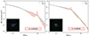 |
Fig. B.1. Surface brightness profile for cluster CL0005_1 seen from two different line of sight. The orange data point refers to the measured emission, the blue line refers to the fitted β-profiles combination model. The emission peaks correspond to the substructure emission: in the projection reported in the left figure the substructure appears in the outer regions of the cluster (R ∼ R500), while in the projection reported on the right the substructure appears near the central core. The difference between the fitted profile and the observed one can be quantified by the colored area that is larger when the substructure appears far from the central core, which means that if the substructure appear far from the central core the observed density profile results much more overestimated. |
Moreover, as shown in Section 4.2 and Section 4.1 the overestimation of the density profiles increases gradually with the radius, in particular in the complete sample and for the irregular clusters, showing that this effect is due to substructures. This radial variation of the density bias can be explained through the two effects just outlined. In fact, if we consider a projection where the substructure appears far from the central core, where the cluster main emission is lower (Figure B.1, left), the substructure emission peak emerges from the main emission profile much more than the case when the same substructure appears near the central core (Figure B.1, right). In this way, the overestimation of the surface brightness, thus the overestimation of the density profile, is higher for larger radii, as shown by the colored areas in Figure B.1. Therefore, if we consider a sample in which substructures can appear at any distance from the core, the bias on the global density profile does increase with the radius.
Appendix C: Shape estimator
We define the shape estimator, a quantity that can evaluate the presence of substructures. For each cluster the shape estimatorSE is defined as:
 (C.1)
(C.1)
where σSB(ri) is the scatter of the surface brightness profiles (normalized over the mean value) measured from the 40 different lines of sight, evaluated at R = ri. Substructures produce an alteration in the surface brightness profile by introducing an SB peak where the substructure appears, so that in that region the surface brightness scatter is higher. The scientific aim of this estimator is to identify the most extreme cases in our sample. Its calibration for a more general use is beyond the scope of this work.
We report in Figure C.1 the scatter at different radii for each cluster in the sample. The σSB(ri) distribution clearly becomes broader as the radius increases: this is due to the fact that in the inner regions substructures are not very distinguishable from the central core since their emission is weaker than the central core, so that the 40 surface brightness profiles of each clusters are very similar to each other, thus the scatter is small; if the substructure appear in the outer regions its emission peak is more evident so that the scatter is higher. Moreover, the latter consideration applies only to irregular clusters (i.e. clusters that present substructures), while for regular clusters the surface brightness profile is not affected by emission peak, so that the scatter remains small regardless of the radius. For example, if we consider CL0035_a its scatter goes from σSB(R = 0.1R500) = 0.05 to σSB(R = 2R500) = 1.9, while CL0129_a goes from σSB(R = 0.1R500) = 0.02 to σSB(R = 2R500) = 0.2. Therefore we can conclude that CL0129_a is more regular than CL0035_a.
 |
Fig. C.1. Scatter of the surface brightness profiles distribution (over the 40 line of sight) for each cluster at different radii. The scatters distribution becomes broader with increasing radius. |
In Figure C.2 we show the shape estimatorSE in ascending order, so that the clusters can be considered in "regularity" order. As we can expect, the sample shows a continuous distribution of SE, which means that the sample presents a varied morphology composition. We can therefore consider the sample as representative of a common cluster population.
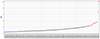 |
Fig. C.2. Shape estimator for each cluster in the sample, showed in ascending order, from the most regular to the most irregular. The blue clusters compose the regular sub-sample, the red clusters compose the irregular sub-sample. |
We chose the first 15 clusters as the regular sub-sample and the last 15 as the irregular sub-sample. In Figure C.3 we report four clusters of each sub-sample that show the validity of the method just defined: the clusters of the regular sample do not show any substructure and present a regular central core, while the irregular sample clusters show complex morphology.
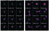 |
Fig. C.3. Example of clusters that compose the regular (left) and the irregular (right) sub-sample. For each clusters we report three different lines of sight (i.e. each column is a different sample realization). The solid and dashed circles represent respectively R500 and 2R500. |
All Tables
Results of the analysis for the biases on the global density profile and on the intrinsic scatter of a cluster population.
All Figures
|
Fig. 1. Mass distribution of the sample of simulated clusters used in this work. The minimum and maximum values of the mass are 2.0 × 10¹⁴ M⊙ and 14.3 × 10¹⁴ M⊙, respectively. |
| In the text | |
|
Fig. 2. Image gallery of the 98 galaxy clusters in the simulated sample. Each image covers an area of 5R500 × 5R500 and represents the spatial distribution of the ICM projected along one random direction in units of cm−6 Mpc. The solid circle indicates R500, while the dashed one indicates 2R500. In many clusters one or more substructures are present. The names of the simulated clusters are reported in each panel. The first number identifies the simulated region where the halo is extracted, and the second is the mass-rank index of the halo in that specific region. For example, CL0005_1 is the most massive cluster found in the fifth region. |
| In the text | |
|
Fig. 3. Representation on a sphere (left) and on a polar plane (right) of the forty directions along which a three-dimensional simulated cluster is projected. The directions are distributed at intervals of Δθ = 1/10 π and Δϕ = 1/8 π, with θ ∈ [0, 9/10 π] and ϕ ∈ [0, 3/8 π], where ϕ = 0 identifies the equatorial plane. Every direction is identified as (t, p), where t ∈ [0, 9] and p ∈ [0, 3] represent θ and ϕ. |
| In the text | |
|
Fig. 4. Mock map generation process. Left panel: Map of the cluster emission. Central panel: Map of the cluster emission with the addition of the tiled background. Right panel: Map resulting from the discretization of the cluster+background map through a Poisson randomization. All maps are in units of counts. |
| In the text | |
|
Fig. 5. Schematic representation of the procedure described in Sects. 2.2.2 and 3 to derive the gas density bias and the intrinsic scatter due to the spherical assumption. |
| In the text | |
|
Fig. 6. Gas density profile along 40 lines of sight for two clusters chosen as examples. In the left figure, the regular cluster CL0129_1 is reported, while the right figure presents the irregular cluster CL0005_1. For both figures, the black line refers to the input gas density profile, and the colored lines refer to the observed profiles, extracted assuming spherical geometry for the gas spatial distribution. Each color refers to a specific line of sight, as reported on the polar plane. In the bottom panel of both figures, the observed-to-input ratio is reported for each line of sight. It is evident how the input profile is better reconstructed for the regular cluster. On the right of each figure, three cluster projections are reported (the color of the edges identifies the corresponding line of sight). The solid and the dashed circles refer respectively to R500 and 2R500. We note the smooth shape of CL0129_1, regardless of the projection, and the irregular shape of CL0005_1, where the substructure position changes with the projection. |
| In the text | |
|
Fig. 7. Characterization of the bias introduced by the spherical assumption for the whole sample. Left figure: Bias in ICM density profile due to spherical assumption. In the bottom panel, we report the zoom of the innermost region. The gray lines refer to the global density profile for each sample realization (one for each line of sight), the solid black line refers to the mean over the sample realizations, and the dash-dotted lines refer to the 1σ value. Right figure: Scatter profile of the sample’s density profiles around the global density profile (upper panel) and the relative bias due to the spherical assumption (bottom panel). The lighter black lines refer to the scatter profile for each sample realization, the solid black line to the mean over the sample realizations, and the dash-dotted lines to the 1σ value. The black dashed line refers to the input profile, and the green dashed line refers to the 50% level. |
| In the text | |
|
Fig. 8. Comparison between each projected SB profile distribution of a regular (left panel) and irregular (right panel) cluster. The regular cluster maps appear very similar to each other despite the projection, so all the SB profiles that refer to different lines of sight present a similar behavior as well and thus show a narrow distribution. On the other hand, the irregular cluster appears very different depending on the considered projection, so its SB profile presents different shapes, making the profile distribution scatter considerable (depending on the radius). |
| In the text | |
|
Fig. 9. Same as Fig. 7 but for the regular and irregular subsamples. Left figure: Bias in ICM density profile due to the spherical assumption. In the bottom panel, the zoom of the innermost region is reported. Right figure: Scatter profile of each sample’s density profiles around the global density profile (upper panel) and the relative bias due to the spherical assumption (bottom panel). The black lines refer to the complete sample, the red lines to the irregular sample, and the blue lines to the regular sample. The lighter lines refer to the global density profile for each sample realization (one for each line of sight), the solid lines to the mean over the sample realizations, and the dash-dotted lines to a 1σ value. In the right figure, the dashed lines refer to the input profile; the green dashed line refers to the 50% level. |
| In the text | |
|
Fig. B.1. Surface brightness profile for cluster CL0005_1 seen from two different line of sight. The orange data point refers to the measured emission, the blue line refers to the fitted β-profiles combination model. The emission peaks correspond to the substructure emission: in the projection reported in the left figure the substructure appears in the outer regions of the cluster (R ∼ R500), while in the projection reported on the right the substructure appears near the central core. The difference between the fitted profile and the observed one can be quantified by the colored area that is larger when the substructure appears far from the central core, which means that if the substructure appear far from the central core the observed density profile results much more overestimated. |
| In the text | |
|
Fig. C.1. Scatter of the surface brightness profiles distribution (over the 40 line of sight) for each cluster at different radii. The scatters distribution becomes broader with increasing radius. |
| In the text | |
|
Fig. C.2. Shape estimator for each cluster in the sample, showed in ascending order, from the most regular to the most irregular. The blue clusters compose the regular sub-sample, the red clusters compose the irregular sub-sample. |
| In the text | |
|
Fig. C.3. Example of clusters that compose the regular (left) and the irregular (right) sub-sample. For each clusters we report three different lines of sight (i.e. each column is a different sample realization). The solid and dashed circles represent respectively R500 and 2R500. |
| In the text | |
Current usage metrics show cumulative count of Article Views (full-text article views including HTML views, PDF and ePub downloads, according to the available data) and Abstracts Views on Vision4Press platform.
Data correspond to usage on the plateform after 2015. The current usage metrics is available 48-96 hours after online publication and is updated daily on week days.
Initial download of the metrics may take a while.