| Issue |
A&A
Volume 693, January 2025
|
|
|---|---|---|
| Article Number | A179 | |
| Number of page(s) | 25 | |
| Section | Extragalactic astronomy | |
| DOI | https://doi.org/10.1051/0004-6361/202452400 | |
| Published online | 17 January 2025 | |
Eppur si muove: Evidence of disc precession or a sub-milliparsec SMBH binary in the QPE-emitting galaxy GSN 069
1
Centro de Astrobiología (CAB), CSIC-INTA, Camino Bajo del Castillo s/n, 28692 Villanueva de la Cañada, Madrid, Spain
2
Universität Zürich, Institut für Astrophysik, Winterthurerstrasse 190, CH-8057 Zürich, Switzerland
3
INFN, Sezione di Milano-Bicocca, Piazza della Scienza 3, I-20126 Milano, Italy
4
Università degli Studi di Milano-Bicocca, Piazza della Scienza 3, I-20126 Milano, Italy
5
Kavli Institute for Astrophysics and Space Research, Massachusetts Institute of Technology (MIT), Cambridge, MA, USA
6
Telespazio UK for the European Space Agency (ESA), European Space Astronomy Centre (ESAC), Camino Bajo del Castillo s/n, 28692 Villanueva de la Cañada, Madrid, Spain
7
European Space Agency (ESA), European Space Astronomy Centre (ESAC), Camino Bajo del Castillo s/n, 28692 Villanueva de la Cañada, Madrid, Spain
8
Center for Astrophysics | Harvard & Smithsonian, 60 Garden Street, Cambridge, MA 02138, USA
9
Department of Physics and Columbia Astrophysics Laboratory, Columbia University, New York, NY 10027, USA
10
Institute for Advanced Study, 1 Einstein Drive, Princeton, NJ 08540, USA
⋆ Corresponding author; This email address is being protected from spambots. You need JavaScript enabled to view it.
Received:
27
September
2024
Accepted:
20
November
2024
Abstract
X-ray quasi-periodic eruptions (QPEs) are intense soft X-ray bursts from the nuclei of nearby low-mass galaxies typically lasting about one hour and repeating every few hours. Their physical origin remains a matter of debate, although so-called impact models appear promising. These models posit a secondary orbiting body piercing through the accretion disc around the primary supermassive black hole (SMBH) in an extreme mass-ratio inspiral (EMRI) system. In this work, we study the QPE timing properties of GSN 069, the first galactic nucleus in which QPEs have been identified. We primarily focus on observed minus calculated (O–C) diagrams. The O–C data in GSN 069 are consistent with a super-orbital modulation of several tens of days, whose properties do not comply with the impact model. We suggest that rigid precession of a misaligned accretion disc or, alternatively, the presence of a second SMBH forming a sub-milliparsec binary with the inner EMRI is needed to reconcile the model with the data. In both cases, the quiescent accretion disc emission should also be modulated on similar timescales. Current X-ray monitoring indicates that this might be the case, although a longer baseline of higher cadence observations is needed to confirm the tentative X-ray flux periodicity on firm statistical grounds. Future dedicated monitoring campaigns will be crucial to test the overall impact-plus-modulation model in GSN 069 and in analogy between the two proposed modulating scenarios. If our interpretation is correct, QPEs in GSN 069 represent the first electromagnetic detection of a short-period EMRI system in an external galaxy, paving the way to future multi-messenger astronomical observations. Moreover, QPEs encode unique information on SMBHs inner environments, which can be used to gain insights on the structure and dynamics of recently formed accretion flows and to possibly infer the presence of tight SMBH binaries in galactic nuclei.
Key words: accretion / accretion disks / black hole physics / galaxies: individual: GSN 069 / galaxies: nuclei / X-rays: general
NASA Einstein Fellow.
© The Authors 2025
 Open Access article, published by EDP Sciences, under the terms of the Creative Commons Attribution License (https://creativecommons.org/licenses/by/4.0), which permits unrestricted use, distribution, and reproduction in any medium, provided the original work is properly cited.
This article is published in open access under the Subscribe to Open model. This email address is being protected from spambots. You need JavaScript enabled to view it. to support open access publication.
1. Introduction
Extreme-variability events associated with supermassive black holes (SMBHs) in galactic nuclei have conistently been detected with increasing frequency in recent years. Recurring optical, UV, and X-ray events, which often show signs of a periodic or quasi-periodic repetition pattern, have been revealed thanks to the extended baseline of follow-up observations. Some of these repeating nuclear transients (RNTs) likely result from the partial stripping (or disruption) of a stellar orbiting companion at pericentre. A few examples include: ASASSN-14ko, an optically detected RNT with mean recurrence time of ≃115 d (Payne et al. 2021, 2022; Bandopadhyay et al. 2024a); eRASSt J045650.3-203750, an X-ray and UV RNT with a recurrence time that decayed from ≃300 d to ≃190 d in about 30 months (Liu et al. 2023, 2024); and Swift J023017.0+283603, which exhibited recurrent X-ray bursts every ≃22 d for a period of few hundred days (Evans et al. 2023; Guolo et al. 2024; Pasham et al. 2024a). On shorter timescales, fast, high-amplitude soft X-ray bursts known as X-ray quasi-periodic eruptions (QPEs) have been unveiled in the past few years from the nuclei of low-mass galaxies (for the first detection, see Miniutti et al. 2019).
Whether the same or similar physical processes give rise to the variety of observed properties and timescales in the current population of quasi-periodic RNTs remains to be understood. On the other hand, most (if not all) of the cases mentioned above are likely associated with the interaction between the central SMBH (or its accretion flow) and orbiting secondary companions in extreme mass-ratio inspiral (EMRI) systems, possibly representing the electromagnetic signature of one promising class of sources of gravitational waves to be detected by future experiments (e.g. Luo et al. 2016; Amaro-Seoane et al. 2017; Babak et al. 2017; Sesana et al. 2021).
In this work, we focus on the relatively novel phenomenon of X-ray QPEs, first discovered in the nucleus of the galaxy GSN 069 (Miniutti et al. 2019). X-ray QPEs are high-amplitude soft X-ray bursts repeating on timescales of hours to days that stand out with respect to an otherwise stable quiescent X-ray emission, likely coming from the accretion disc around a SMBH. Following their detection in GSN 069, QPEs have been identified in another eight galactic nuclei (Giustini et al. 2020; Arcodia et al. 2021, 2024a; Chakraborty et al. 2021; Quintin et al. 2023; Nicholl et al. 2024). So far, QPEs are exclusively detected in the X-rays and no counterpart has been observed in the radio, IR, optical, or UV (see Linial & Metzger 2024a for theoretical predictions regarding UV-QPE analogues).
The X-ray spectral properties of QPEs in the different sources studied so far are remarkably similar. Their X-ray spectrum is thermal-like with typical temperature evolving from kT ≃ 50–80 eV to ≃100–250 eV and back during the event. The spectral evolution during bursts suggests an expanding emitting region (assuming blackbody emission). Overall, QPEs have a duty cycle (QPE duration over out-of-QPE quiescence) of 10–30% and their X-ray luminosity at peak is 1042–1043 erg s−1, depending on the specific source. During each QPE, hysteresis is present in the LX-kT plane, with a hotter rise than decay (see e.g. Arcodia et al. 2022; Miniutti et al. 2023a; Quintin et al. 2023; Chakraborty et al. 2024; Giustini et al. 2024; Nicholl et al. 2024).
The nuclear optical spectra of QPE host galaxies exhibit narrow emission lines with properties indicating the presence of an ionising source in excess of pure stellar light (Wevers et al. 2022). Despite being basically unobscured in the X-rays, none of the current QPE-emitting galaxies show any optical or UV broad emission lines in their spectra. This rules out the presence of a currently active galactic nucleus and supports the notion that the quiescent emission seen in the X-rays is associated with an accretion flow that is unable to sustain a mature broad line region, possibly as a result of being too compact. Velocity dispersion measurements from optical spectroscopy indicate black hole masses of 105 − 106.5 in QPE galactic nuclei with the possible exception of an higher mass of ≃1 − 7 × 10⁷ M⊙ in eRO-QPE4 (Arcodia et al. 2024a).
Recent studies have revealed a connection between QPEs and tidal disruption events (TDEs). The long-term evolution of the quiescent X-ray emission in GSN 069 is consistent with a long-lived TDE peaking around July 2010 and with a second, partial TDE 9 yr later, although the latter interpretation is likely not unique (Miniutti et al. 2023a). GSN 069 also shows abnormal C/N ratio in its UV and X-ray spectra (Sheng et al. 2021; Kosec et al. 2025), which is consistent with a TDE interpretation, possibly from an evolved or stripped star (Mockler et al. 2024). The recently confirmed QPE source AT2019vcb (Quintin et al. 2023; Bykov et al. 2024), also known as Tormund, was initially detected as an optical TDE (Hammerstein et al. 2023) and XMMSL1 J024916.6-041244 (Chakraborty et al. 2021) was classified, prior to QPE identification, as an X-ray-detected TDE (Esquej et al. 2007). The X-ray decay of the quiescent emission in eRO-QPE3 is also suggestive of a TDE (Arcodia et al. 2024a). The recently reported QPEs in AT2019qiz occur in a well studied optically-selected TDE and were first detected about 4 yr after optical peak (Nicholl et al. 2024), confirming a clear connection between QPEs and TDEs as well as a likely delay in their appearance with respect to the TDE outburst, as noted already in GSN 069 by Miniutti et al. (2019). Finally, QPEs and TDEs appear to prefer the same type of low-mass, post-starburst host galaxies with a high incidence of extended narrow line regions (Wevers et al. 2024; Wevers & French 2024), pointing towards a scenario in which the nuclei of QPE galaxies were active in the past but have then switched off leaving only relic narrow emission lines, as suggested by Miniutti et al. (2019) for GSN 069, whose optical spectrum is unambiguously that of a Seyfert 2 galaxy (Miniutti et al. 2013; Wevers et al. 2022). This is also consistent with the analysis of Hubble Space Telescope data of GSN 069 by Patra et al. (2024), highlighting the presence of a compact (≲35 pc) [O III] emitting region that is likely ionised by the current, recently activated emission. High-cadence X-ray monitoring of TDEs, especially at late times, may thus be key to discover new QPE-emitting galactic nuclei.
The physical origin of QPEs is still uncertain and the focus of active research. Several models have been proposed so far, and they cluster into two main scenarios: disc instability models (Raj & Nixon 2021; Pan et al. 2022, 2023; Śniegowska et al. 2023; Kaur et al. 2023), and orbital models invoking the repeated interaction between the central SMBH and orbiting companions (see e.g. King 2020, 2022; Ingram et al. 2021; Suková et al. 2021; Metzger et al. 2022; Krolik & Linial 2022; Zhao et al. 2022; Wang et al. 2022; Lu & Quataert 2023; Linial & Sari 2023; Wang 2024). In this work, we focus on the QPE timing properties in GSN 069 and we compare the timing behaviour to the theoretical predictions from one of the most popular QPE models: this is the so-called impact model that invokes repeated collisions between an orbiting companion and the accretion disc around the primary SMBH in an EMRI system, with each collision giving rise to an X-ray QPE (Xian et al. 2021; Linial & Metzger 2023; Franchini et al. 2023; Tagawa & Haiman 2023; Zhou et al. 2024a,b; Yao et al. 2025).
After introducing a few relevant definitions in Section 2, we study the QPEs timing properties in GSN 069 in Sections 3 and 4. The impact model for QPEs is introduced in Section 5, where we discuss its predictions in comparison with the GSN 069 data highlighting a series of inconsistencies that can be cured by introducing an external modulation of QPEs arrival times. Two possible modulation scenarios are proposed in Section 6, while Section 7 offers a discussion of the current status on SMBH mass estimates in GSN 069. The two proposed modulation scenarios are compared with the data in Sections 8 and 9 by making use of numerical simulations of impact times between the secondary and the accretion disc around the primary SMBH. The quiescent (out-of-QPEs) X-ray flux variability from an X-ray monitoring campaign between May and September 2024 is studied in Section 10. We discuss our results and their implications in Sections 11 and 12.
2. QPE timing definitions
Models invoking twice-per-orbit collisions between a secondary object (a star or black hole) and the accretion disc around the primary SMBH in an EMRI system have received considerable attention in the recent past. These approaches have mainly been based on the alternating longer and shorter recurrence times between consecutive QPEs in GSN 069, RX J1301.9+2747, and eRO-QPE2, as well as on the presence of an X-ray quiescence consistent with accretion disc emission (Miniutti et al. 2019; Giustini et al. 2020; Arcodia et al. 2021). In this work, we introduce a few definitions that can be derived from QPEs peak times of arrival and that are well suited to study the QPE timing properties within the context of the impact model. As a note of caution, we point out that the intrinsic (unknown) delay between a collision and the corresponding QPE peak emission was assumed not to vary across impacts in this work. Under this assumption, the QPE arrival time is therefore taken as representative of the corresponding impact time. We stress that the amplitude of the delay itself is not relevant, as our analysis is based on differential quantities (e.g. the recurrence time between QPEs), but delays becomes potentially important if they vary across impacts. The notion that delays are independent of impacts is not necessarily correct, so that all results presented in our work are likely subject to a certain degree of systematic error. Thus, the reported statistical uncertainties should be considered with some caution.
In Fig. 1, we show a schematic representation of a QPE time series comprising four consecutive QPEs where we define, for any QPE at time ti, the QPE recurrence time Trec, the EMRI apparent orbital period (Papp), and its apparent eccentricity (eapp) as:
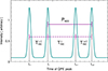 |
Fig. 1. Schematic representation of a QPE time series comprising four consecutive QPEs. Odd and even QPEs represent impacts through the ascending and descending nodes respectively (or vice versa). The definition of the different QPE recurrence times that are used to compute Papp and eapp is highlighted (see Eqs. (1)–(3) and text for details). |
 (1)
(1)
 (2)
(2)
 (3)
(3)
In the context of the impact model, odd and even QPEs are associated with collisions between the secondary EMRI component and the accretion disc around the primary at the ascending and descending nodes respectively (or vice versa). The time interval Papp between consecutive QPEs of the same parity thus provides an estimate of the EMRI orbital period Porb. Consecutive QPEs of different parity are instead separated by alternating longer and shorter Trec, unless the EMRI orbit is circular or the intersection between the disc and the orbital planes lies along the orbit’s semi-major axis. By definition, eapp is an apparent EMRI eccentricity; for Keplerian orbits, this is constant and can take any value between zero and  , depending on the system geometry. The maximum
  is reached when the difference between consecutive longer and shorter recurrence times is the largest, that is, when the intersection between the orbital and disc planes is along the orbit’s latus rectum. As a consequence, a measure of
  represents a lower limit on the actual orbital eccentricity, eorb.
In general relativity, the apsidal precession of the EMRI orbit implies that Trec, Papp, and eapp vary periodically on the apsidal precession timescale. Therefore, Papp is not equal to the constant Keplerian orbital period, while eapp spans all possible values between zero and  , depending on precession phase. In fact, eapp ≃ 0 twice per apsidal period, that is when consecutive impacts occur close to apocentre and pericentre. A schematic view of the effects of apsidal precession on the impacts between the EMRI’s secondary and the disc is shown in Fig. 2. We note that due to the different location of impacts on the disc with respect to the observer, light-travel time delays have to be expected as well. Considering a typical EMRI nearly circular orbit with semi-major axis of 100 Rg, and a SMBH mass of 106 M⊙, light-travel time delays are expected not to exceed 103 s, or ≃17 minutes. However, such relatively large delays are only obtained for the specific geometry in which impacts are aligned with the line of sight and occur close to apocentre and pericentre, respectively. More generally, light-travel time delays are not expected to exceed a few minutes. The impact model predictions on all the quantities defined above are discussed and compared with the observed QPE data of GSN 069 in Section 5.
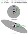 |
Fig. 2. Effects of apsidal precession on secondary-disc impacts. We show two different apsidal phases leading to |

3. Application to GSN 069
We considered QPE data of GSN 069 and we derived, from the observed X-ray light curves, the quantities defined in Eqs. (1)–(3) from the observed QPEs peak times. Details on the observations used in this work and on relevant aspects of data analysis are given in Appendix A. Here, we make use of the first four observations during which QPEs were detected, from December 2018 to May 2019. Soon after, the quiescent (out-of-QPEs) X-ray emission of GSN 069 experienced a sudden significant rebrightening, peaked for about 200 d, and started to decay towards the previous X-ray flux level. QPEs were detected during the rise, disappeared at peak, and were detected again during the decay, but with timing properties significantly different from those preceding the rebrightening (Miniutti et al. 2023a,b). As discussed by Miniutti et al. (2023b), the disappearance of QPEs at peak is not because they are overwhelmed by enhanced disc emission, but is rather associated with a significantly lower QPE peak temperature that approaches that of the quiescent disc emission. As an example, in observations with the highest quiescent level and no QPEs, the quiescent 0.2–1 keV count rate is ≃0.7 cts s−1, significantly lower than the typical QPE peak count rate (typically ≳1.5 cts s−1 in the same band), so that QPEs with similar amplitude and, most importantly, temperature as those that are observed at lower flux levels would have been easily detected. On the other hand, if the QPE peak temperature is similar to that of the underlying disc emission at high disc fluxes (or, better, at high mass accretion rates), QPEs would be observed as low-amplitude X-ray fluctuations since their bolometric luminosity is a relatively small fraction of the disc one (Miniutti et al. 2023a,b).
The X-ray rebrightening was consistent with a second partial TDE occurring about 9 yr after the initial one in GSN 069, although this interpretation is only based on the X-ray light curve shape and, thus, it is unlikely to be unique. Partial rather than full TDEs might also contribute to explain the long-lived nature of the X-ray emission in GSN 069 following its initial 2010 X-ray outburst (Bandopadhyay et al. 2024b). The irregular QPE properties during the rebrightening rise and decay might then signal that the accretion flow was disturbed, re-arranging, and possibly rapidly precessing at that epoch (see e.g. Linial & Metzger 2024b), and could support QPE models in which the disc plays an important role, such as the impact model. The properties of the QPEs detected after May 2019 are being studied in detail and will be presented in a forthcoming work, although some relevant results are anticipated in Section 4.2.
Figure 3 shows Trec, Papp, and eapp values for the four observations of GSN 069 considered here, together with the corresponding X-ray light curves. All quantities were derived from QPEs peak times of arrival obtained through constant plus Gaussian functions fits to the corresponding X-ray light curves, as briefly discussed in Appendix A. The recurrence times between consecutive QPEs consistently alternate defining longer and shorter consecutive Trec, as expected in the impact model for any non-zero EMRI eccentricity. We note that longer recurrence times always follow stronger QPEs, although this could be chance coincidence due to the limited number of detected QPEs (15). The separation between QPEs of the same parity (Papp, a proxy for the EMRI’s orbital period) is not constant. Finally, eapp is also variable with typical values suggesting that the EMRI eccentricity is low but non-zero in GSN 069. This is in agreement with results by Franchini et al. (2023) and Zhou et al. (2024b) who have applied different versions of the impact model1 to GSN 069 deriving an EMRI’s orbital period of Porb ≃ 18 h and eccentricity of either ≃0.1 or ≲0.15, both consistent with the average Papp and with eapp in Fig. 3.
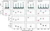 |
Fig. 3. QPE timing properties in GSN 069. In the upper row, we show the X-ray 0.4–1 keV light curves of GSN 069 used in this work. The first two and last light curves are from the EPIC-pn camera on board XMM-Newton, while the third is from the ACIS-S detector on board Chandra. The latter light curve has been re-scaled to the expected EPIC-pn count rate (as in Miniutti et al. 2023a). XMM-Newton data could be used down to 0.2 keV but, since QPE properties (peak time and overall duration) are energy-dependent (Miniutti et al. 2019), we use here a common energy band down to 0.4 keV only in order to make use also of the Chandra data. The three lower rows show Trec, Papp, and eapp as obtained from the QPE peak times. Due to the gaps in the data the colour code distinguishing odd from even QPEs during different observations might be different from the one shown here where we arbitrarily assigned all stronger (weaker) QPEs to the even (odd) time series. |
4. O–C analysis
A further quantity that is useful when dealing with periodic or quasi-periodic time series is the difference between Observed and Calculated (O–C) times of arrival of events (here QPEs) as a function of time (or epoch). “O” stands for the observed time of arrival of QPEs with respect to a chosen reference, while “C” is their expected time of arrival assuming that events are all separated by the same trial period Ptrial. The O–C analysis is a powerful tool to identify deviations from strictly periodic behaviour and is widely applied in the analysis of time series from variable stars, eclipsing binaries, or exoplanet’s transits (for basic definitions, see Sterken 2005). A strictly periodic time series produces linear O–C diagrams, where the slope is related to the difference between the true period Ptrue and the trial one Ptrial. The presence of a constant period derivative Ṗ produces an additional parabolic term in O–C diagrams, and its coefficient can be used to estimate the actual Ṗtrue. Besides these standard functional forms, O–C diagrams can help identify further deviations from periodic behaviour. Within the impact model scenario, O–C diagrams need to be computed for odd and even QPEs separately as those are the events that are expected to be separated by a constant period (the EMRI orbital one) at least at the Keplerian level while, as already mentioned, consecutive QPEs of different parity are generally separated by alternating longer and shorter intervals.
4.1. O–C diagrams for GSN 069
Before discussing O–C diagrams for GSN 069, some caveats must be spelled out. In order to construct O–C diagrams, one has to first select a reference event together with an assumed trial period Ptrial, and then derive the correct epoch (i.e. number of elapsed Ptrial) for all other events with respect to the reference one. For continuous time series this is a trivial exercise, but the GSN 069 data considered here comprise four observations with typical duration of the order of 0.5 − 1.5 d separated by ∼23 d, ∼29 d, and ∼107 d respectively. The data gaps introduce some degree of ambiguity in the correct QPE identification (number of elapsed Ptrial with respect to the reference one).
We have therefore constructed a number of different versions of O–C diagrams for different QPE identifications, We defined the first two QPEs observed in December 2018 (see Fig. 3) as reference for odd and even QPEs respectively, and we assumed as Ptrial the average measured Papp = 17.88 h throughout the ≃160 d campaign. QPEs belonging to the January 2019 observation are unambiguously identified, while those detected in February and May 2019 cannot be uniquely associated with the odd or even time series and with a specific number of elapsed Ptrial. The uncertainties in QPE epoch and parity are unavoidable and due to the sparse nature of the data and the relatively long gaps with respect to Ptrial.
However, in this work we are interested in comparing the QPE timing properties with the specific impact model which implies that odd and even QPEs need to share the same period (and period derivative, if present) as this is uniquely associated with the EMRI orbital period Porb (and Ṗorb). Hence, at zeroth-order, the O–C data for odd and even QPEs must be described by standard O–C functional forms (linear or linear plus parabolic) with the same coefficients. We therefore considered as acceptable only O–C diagrams that fulfil this condition. By imposing this requirement, the ambiguity in the identification of QPEs was significantly reduced, at the expense that results presented below are not entirely model-independent.
Despite our assumptions, the identification of QPEs from the last (May 2019) observation, the one associated with the longest gap in the data, remains uncertain since different identifications produce O–C diagrams that comply with our requirements. This ambiguity is associated with two possible sources of error: if an event (from the May 2019 data set) is associated with the odd time series but actually belongs to the even one (or vice-versa), all O–C data for that observation are shifted upwards or downwards by the average time separation between consecutive odd and even QPEs (Trec), namely, half Ptrial. On the other hand, if the parity assigned to a given event is correct but the epoch (number of elapsed Ptrial) misidentified by one, all data points shift by one Ptrial. We have therefore produced three versions of the O–C diagrams for GSN 069 that differ by the identification of QPEs during the May 2019 observation. We discuss here the identification that produces intermediate O–C values for the May 2019 observation, while two other possibilities, for which O–C data are shifted upwards or downwards with respect to the case discussed here, are presented in Appendix B.
The upper panels of Fig. 4 show the resulting O–C data for odd (left) and even (right) QPEs, where events of different parity are shown in separate panels for visual clarity (data points overlap at the chosen symbol size). We applied standard O–C models to the data; as mentioned, a linear trend is expected for strictly periodic time series, while the addition of a parabolic decay signals the likely presence of a period derivative. It was immediately clear that the data could be described by a linear plus parabolic trend at zeroth-order, but that a sinusoidal-like modulation was also likely present. A model of the form a + bx + cx2 + Amodsin(Pmod, ϕmod) was found to describe the data well, although the sparse nature of the data prevented us to distinguish between two possible modulating periods of ∼19 d and ∼43–44 d. It is worth noting that, due to the limited number of data points in the odd QPEs time series (six, as are the free parameters of the adopted model), the model could not be formally applied in that case. The adopted fitting procedure is described in Appendix B.
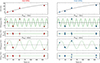 |
Fig. 4. O–C diagrams for GSN 069. We show the O–C diagrams for odd (left) and even (right) QPEs for GSN 069 resulting from identifying the first QPE of the May 2019 observation with the 211th even QPE. The upper panels show the O–C data together with the linear plus parabolic baseline model for Pmod ≃ 19 d. The lower panels show the corresponding residuals (O–CBASELINE) as well as the ones corresponding to the full best-fitting model including a sinusoidal modulation (O–CFULL) for the two possible Pmod. The sinusoidal modulation is also shown in the O–CBASELINE to guide the eye. |
The solid line in the upper panels of Fig. 4 is the linear plus parabolic part of the best-fitting relation for the Pmod ∼ 19 d modulation (the relation for the ∼43–44 d modulation is consistent with it within errors and is not shown for visual clarity). In the lower panels, we show the O–C residuals once the baseline linear plus parabolic best-fitting model is subtracted (O–CBASELINE) as well as those resulting from the subtraction of the full best-fitting model (O–CFULL). For both possible Pmod, the shape of O–CBASELINE is well described by a sine function (shown to guide the eye), as demonstrated by the small residuals shown in O–CFULL in both cases. Results from the O–C analysis are given in Table 1, where we report as free parameters the physical Porb and Ṗorb (the EMRI orbital period and derivative) that are derived unambiguously from the coefficients of the linear and quadratic terms of the adopted model. The two best-fitting modulating periods are well defined in Δχ2 space, as shown in Fig. 5. Other local minima in Δχ2 space were not well behaved, with large fluctuations around the local minimum.
O–C analysis for GSN 069.
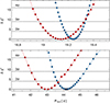 |
Fig. 5. Pmod detection in the O–C diagrams. We show Δχ2 as a function of modulating period Pmod for the final best-fitting model to the O–C diagrams in Fig. 4. Odd QPEs are shown in red, even ones in blue. We explored a wide range of Pmod between 4 d and 90 d, and all other local minima are noisy (i.e. neighbouring data points to the local minimum have much higher Δχ2 value). |
The ∼19 d modulating periods for odd and even QPEs are consistent with each other at the 2σ level, while only marginally so for the longer period. However, as already mentioned in Section 2, we stress again that the uncertainties reported in Table 1 (and shown in Fig. 5 for the case of Pmod) are statistical only. Within the framework of the impact model, the O–C analysis should be carried over the actual (unknown) impact times, while we have used the QPE (peak) times of arrival. This introduces systematic errors, as there is no guarantee that the delay between an impact and the peak of the corresponding X-ray emission is impact-independent. Hence, we caution that the uncertainties reported in Table 1 are likely underestimated, and we discourage to consider our measurements as accurate at better than the few per cent level. This is the reason why we accept as plausible the 43–44 d modulation despite a marginal discrepancy in the period derived from odd and even QPEs time series.
For both odd and even QPEs, the coefficients of the linear and quadratic terms are consistent with each other regardless of the actual modulating period, indicating that odd and even QPEs have common period P and period derivative Ṗ. The existence of such a solution is fully consistent with, and actually provides some support to, the impact model because the QPE timing properties of both odd and even QPEs are imposed by the EMRI orbital period and its evolution. We point out that, within the impact model scenario, the period derived from the O–C analysis is that of consecutive impact at the same node (draconitic period), rather than the EMRI orbital period. In general relativity, the two periods do not coincide as is the case for Keplerian orbits. However, the difference (due to relativistic corrections associated primarily with apsidal precession) is typically of the order of only few per cent for orbits wider than few tens gravitational radii Rg as is almost certainly the case here (Linial & Metzger 2023; Franchini et al. 2023), so that the derived period and period derivative can be considered as estimates of the EMRI Porb and Ṗorb to within few per cent.
As reported in Table 1, we measure an average Porb ≃ 18.07 h and Ṗorb ≃ −3–4 × 10⁻⁵ in GSN 069. The O–C data are modulated on either a ≃19 d or ≃43–44 d timescale with semi-amplitude of the order of 2.5–2.8 h. As discussed in Appendix B, the other two possible identifications for the May 2019 QPEs lead to consistent results for all parameters except Ṗorb which takes the values of Ṗorb = 0 or Ṗorb ≃ −6 –7 × 10⁻⁵ depending on QPE identification. In summary, the EMRI orbital period and the properties of the O–C modulation (although with two possible solutions) are found to be robust against different QPE identifications. The only significant impact is on the derived Ṗorb for which we suggest three possible values, depending on QPE identification in the May 2019 data, namely Ṗorb = 0, −3–4 × 10⁻⁵, or −6–7 × 10⁻⁵.
On the other hand, while parabolic trends in O–C diagrams are ubiquitously interpreted as a period derivative, we point out that this interpretation is not necessarily unique. If the O–C data were in fact modulated also on a further much longer timescale  , their analysis on a baseline significantly shorter than
  could result in the detection of spurious parabolic trends. As an example, if the central SMBH was spinning, nodal precession of the EMRI orbit would modulate the O–C diagrams on a very long timescale, significantly longer than the ∼160 d baseline of the GSN 069 data (see Fig. C.1 and associated discussion). We therefore caution that the Ṗorb values derived above assume that the parabolic trend seen in the O–C diagrams is real and not just the sign of a longer timescale modulation.
4.2. The 2023 campaign: hints for period decay
Timing QPE data obtained at significantly later times than 2019 could, in principle, be used to confirm (or reject) a period decay in GSN 069, perhaps also clarifying the correct version of the three O–C diagrams we have presented above and in Appendix B. As mentioned, after May 2019, GSN 069 experienced a significant X-ray rebrightening and subsequent decay. QPEs disappeared at peak and had irregular properties during rise and decay. These QPEs are not very useful for deriving an averaged period to compare with the 2018–2019 one precisely because of their irregular timing behaviour which is likely due to changes in the disc structure and dynamics at rebrightening (possibly a second partial TDE) rather than in the EMRI’s orbital parameters (see also Linial & Metzger 2024b).
GSN 069 was later re-observed three times by XMM-Newton within ∼1.5 months in 2023, about 3.5 yr after rebrightening. QPEs were detected in all observations and appeared to be more regular than during rebrightening. The XMM-Newton EPIC-pn light curves from these three observations are shown in Fig. 6, where they are also compared with the May 2019 light curve (upper panel). Although still somewhat irregular, the timing pattern appears to approach that of the previous regular phase, represented here by the May 2019 light curve. The alternating Trec behaviour is preserved, and longer recurrence times always follow stronger QPEs, as was the case in the regular phase (see Fig. 3). As visually clear from Fig. 6, the time interval between QPEs of the same parity (Papp) during the 2023 observations is generally shorter than during the May 2019 observation, which could indicate a period decay between the 2019 and 2023 epochs.
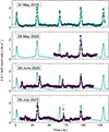 |
Fig. 6. 2023 campaign on GSN 069. In the upper panel, we show the XMM-Newton EPIC-pn light curve from the May 2019 observation, together with a representative best-fitting model. The EPIC-pn light curves from the 2023 campaign are shown in the lower panels. We aligned the last QPEs of these latter observations with one of the QPEs in the upper panel to ease comparison, and we also reproduced the best-fitting model for the May 2019 light curve in the lower panels. |
The number of QPEs detected during the 2023 campaign is insufficient to perform a reliable O–C analysis. However, the light curves in Fig. 6 can be used to derive the average Papp in 2023. As shown in the previous O–C analysis (and confirmed in Appendix B), the difference between ⟨Papp⟩=Ptrial and Porb was found to be of the order of 1% only in 2019. We assume here that the average  h can be taken as representative of
  but with a larger uncertainty of 3% in the attempt to account for the limited number of independent measurements (4) and the somewhat still irregular nature of the 2023 QPE timing. We then derive
  h, so that the difference between the estimated orbital periods in 2023 and 2018–2019 is ΔPorb = −1.4 ± 0.5 h. By taking as reference the mid-point of the time spanned by the 2018–2019 and 2023 observations, the elapsed time between the two campaigns is ΔT ≃ 1560 d, so that we estimate ΔPorb/ΔT = ( − 3.7 ± 1.3)×10−5, or −0.3 ± 0.1 h per year. This is consistent with the inferred
  –4 × 10⁻⁵ from the O–C analysis presented above, and provides some support to results in Table 1 with respect to alternative O–C identifications (see Appendix B). Future monitoring campaigns detecting a sufficiently large number of QPEs to perform detailed O–C analysis on relatively long baselines will be extremely valuable to confirm (or reject) the suggested EMRI period derivative in GSN 069 that we consider, at present, tentative only.
5. The impact model: Timing properties and comparison with GSN 069 data
In order to show the general properties of the impact model, and to compare its predictions with the GSN 069 data, we considered simulations performed using the code developed by Franchini et al. (2023) to which we refer for details (see also Appendix C). Although disc precession can be implemented in their code, we initially switched it off to illustrate the general behaviour of the QPE timing within the context of the simplest version of the impact model.
We selected fiducial parameters for GSN 069 assuming a non-spinning primary SMBH with mass M = 8 × 10⁵ M⊙ forming an EMRI system with a secondary orbiting object of mass m ≪ M. The EMRI’s orbital period was set to 18 h, and the orbital eccentricity to e = 0.05, of the order of those inferred in GSN 069 within the impact model scenario (Franchini et al. 2023; Zhou et al. 2024b). Choosing a different black hole mass keeping an orbital period of 18 h (as set by the data) only changes the EMRI semi-major axis and, as a consequence, the apsidal precession timescale without affecting in any way the general behaviour presented below.
We assumed that the accretion disc around the primary SMBH has angular momentum misaligned by idisc = 5° with respect to the z-axis2, while the EMRI angular momentum vector was set at iEMRI = 10°. The observer inclination with respect to the z-axis was set to iobs = 30°. We point out that different choices of iobs do not significantly affect the results discussed below. As mentioned, no disc precession was included initially and we assumed, for simplicity, Ṗ = 0.
In Fig. 7, we show Trec, Papp, eapp (defined in Eqs. (1)–(3)) and the O–C diagrams from the simulated light curves3. Odd and even QPEs are represented with different colours. Trec and Papp for the two branches are in phase opposition and periodic at the apsidal precession timescale, as discussed e.g. by Linial & Quataert (2024). The anti-correlation of Papp propagates into that of the O–C diagrams for the two branches shown in the lower panels of Fig. 7. This is a well known result in the analysis of O–C diagrams of eclipsing binaries showing apsidal motion, where the anti-correlation between the O–C diagrams of primary and secondary eclipses is ubiquitously observed (Zasche et al. 2014). Due to the symmetric nature of its definition, the distinction between odd and even QPEs disappears in eapp which exhibits a distinctive bell-like shape spanning all allowed values from zero to  and reaching eapp = 0 twice per apsidal period (at each crossing between the Trec, see upper panels of Fig. 7) as illustrated in Fig. 2.
The properties outlined above are not affected significantly by changing any of the system parameters. The only qualitative effect is that induced by a non-zero primary SMBH spin because, even without considering any disc precession, it introduces nodal precession of the EMRI orbital plane, thus affecting the QPE timing. The effects of black hole spin are briefly discussed in Appendix C, and they are ignored in our work because the nodal precession timescale is, for any reasonable choice of parameters, much longer than the apsidal precession one and than that spanned by typical QPE observations, and is of the order of ≃1 yr (Linial & Metzger 2023). Some minor effects are also present on shorter timescales, but they do not modify the qualitative behaviour of the QPE timing we are interested in here, at least on timescales probed by observations. We therefore selected a non-spinning primary SMBH throughout our work, but stress that future implementations attempting to derive physical parameters from the data should also include black hole spin effects self-consistently.
The model’s predictions shown in Fig. 7 can be compared with the observed data shown in Fig. 3 (Trec, Papp, and eapp) and with the O–C diagrams of Fig. 4 (see also Figs. B.1 and B.2). The most striking discrepancy between the model’s prediction and QPE data is that the observed apparent orbital period Papp as well as the O–C diagrams for odd and even QPEs are not in phase opposition. The number of observed consecutive Papp data points is limited (see Fig. 3), but for the data to be consistent with the behaviour shown in Fig. 7, we should have observed GSN 069 precisely when Papp of odd and even QPEs cross in January and May 2019, which appears highly unlikely. As per the O–C data, all three versions of the O–C diagrams that we consider acceptable are indeed modulated at a super-orbital timescale, but the two branches only have marginal phase difference, as clear from e.g. Fig. 4. Moreover, the observed amplitude of the O–C modulation (≃2.5–2.8 h) is about one order of magnitude higher than that induced by apsidal precession which is of the order of few minutes only (see Fig. 7, and compare it with Fig. 4 as well as with with Figs. B.1 and B.2). We point out that none of the O–C diagrams that we have produced, including those that were eventually rejected for not fulfilling our requirements, exhibited odd and even QPEs O–C data in even approximate phase opposition. Further discrepancies are also present for the observed Trec as they indeed alternate as expected from the model, but are not exactly anti-correlated or in phase opposition. As an example, the increase in Trec for the lower branch in May 2019 (red data points in Fig. 3) is much more pronounced than its decay for the upper one (blue data points). Finally, the observed eapp does not not display the typical bell-like shape expected from the model, although this might be a consequence of the limited number of data points and of the relatively short timescales that could be explored continuously.
On the other hand, some of the model expectations are indeed fulfilled by the data. The observed Trec consistently alternate between longer and shorter recurrence times, as natural in the impact model. Moreover, there exist O–C diagrams for which the coefficient of the linear (and parabolic, when needed) part of the best-fitting relation is precisely the same for both odd and even QPEs, indicating that odd and even QPEs share the same period (and period derivative, when present), consistent with expectations. It is therefore plausible that the impact model needs to be modified rather than rejected altogether.
Impacts models with no disc precession, similar to the one discussed above, have been successfully applied by Xian et al. (2021) and Zhou et al. (2024a,b) to multi-epoch observations of GSN 069. Besides the specific parameters (black hole mass and EMRI orbital parameters) that basically affect timescales rather than the qualitative behaviour, their model is equivalent to the one discussed above, whose properties are shown in Fig. 7. Due to the discrepancies highlighted above, the data do not seem to comply with the model’s version implemented in these works (i.e. impact on a geometrically thin disc with no disc precession). On the other hand, Franchini et al. (2023) have qualitatively reproduced one single-epoch light curve of GSN 069 (as well as of other QPE sources) by including a spinning primary SMBH with a misaligned and rigidly precessing accretion disc. Due to the additional ingredient of disc precession, their model cannot be directly compared with Fig. 7 and its ability to reproduce the observed properties highlighted above is studied in more detail in Section 8.
6. Possible way(s) forward
Despite the ambiguities discussed in Section 4, O–C diagrams retain the largest number of useful data points (one per QPE) with respect to all other quantities we have introduced (Trec, Papp, and eapp). They are therefore more informative in deriving trends and in comparing the observed QPE timing properties with model’s predictions, at least at the qualitative level we are interested in here. As an example, the four light curves in Fig. 3 provide 15 O–C data points, but only 11 Trec and 7 Papp and eapp.
Focussing on O–C diagrams, the fact that odd and even QPEs O–C data are modulated periodically with minimal phase difference means that QPEs belonging to one branch are delayed (or anticipated) by the same time interval and with the same sign, as those belonging to the other with respect to an assumed perfect periodicity. These common delays oscillate on a long, super-orbital timescales of ≃19 d or ≃43–44 d in GSN 069. A natural super-orbital timescale is the EMRI apsidal precession, but apsidal motion inevitably makes the two branches oscillate in phase opposition with each other (see Fig. 7) so that, at least in the framework of the impact model, apsidal precession cannot be associated with the observed O–C periodic modulation.
The only plausible way of introducing a correlation between the two branches is that there is a further modulating timescale that dominates, over the observed baseline, with respect to apsidal precession. In particular, such modulating timescale should be shorter than the apsidal one4, and have sufficiently high amplitude for the anti-correlation induced by apsidal precession to be overwhelmed or, at least, to be less dominant.
Within the impact model scenario, there is a natural way of introducing an external periodic modulation. As mentioned, when the primary SMBH is spinning, the orbital plane of the EMRI periodically changes inclination with respect to the plane of the disc due to nodal precession. As discussed in Appendix C and shown in Fig. C.1, this induces a coherent modulation of the O–C diagrams for odd and even QPEs. However, the timescale associated with nodal precession is much longer than the apsidal precession one, so that the latter dominates on short timescales and O–C diagrams for odd and even QPEs are still in phase opposition over the baseline that can be currently probed by observations (say a few apsidal precession timescales). On the other hand, if the SMBH is spinning and the accretion disc misaligned, disc precession can also be present. The effect of disc precession on O–C diagrams is likely similar to that induced by nodal precession of the orbit (see Fig. C.1), but the disc precession timescale can be significantly shorter than the nodal and apsidal ones depending on black hole mass, spin, and disc structure (Franchini et al. 2016), so that it might dominate over apsidal precession and break the expected anti-correlation of O–C diagrams for odd and even QPEs. We explore this possibility in Section 8 below.
On the other hand, QPE light curves are remarkably similar to eclipsing binary ones, only having bursts of X-ray emission rather than eclipses, which in fact motivated initial attempts to model QPEs in terms of self-lensing in an SMBH binary (Ingram et al. 2021) and inspired us to apply the O–C technique to QPEs. One possible source for the observed O–C modulation comes directly from the analogy between the two systems. Apsidal motion is often seen in O–C diagrams of eclipsing binaries, and is in fact identified precisely by the anti-correlation between primary and secondary eclipses in O–C data. However, the O–C diagrams for primary and secondary eclipses do sometimes correlate, which is often identified with light-travel-time effects arising due to the motion of the binary system around the centre of mass with a third orbiting star. In fact, correlated and periodic O–C diagrams have been used to infer the presence of triple systems in many instances (see, for example Zasche et al. 2015). The same idea can in principle apply to QPE data and would imply the presence of an outer SMBH forming a binary with the EMRI plus disc (QPE-emitting) system. Such a hierarchical triple system, comprising an outer SMBH binary and an inner EMRI, is discussed in Section 9 below.
In any case, a qualitative solution to the QPE timing behaviour in GSN 069 must: (i) generally preserve the alternating Trec, although introducing some distortion that breaks the (unobserved) anti-correlation between odd and even QPEs recurrence times; (ii) align the Papp for the two branches on the same (or similar) functional form, again breaking the expected anti-correlation on the apsidal precession timescale; (iii) produce periodic O–C diagrams at some super-orbital timescale in which O–C data for odd and even QPEs have only marginal phase difference.
7. Black hole mass estimates in GSN 069
In the context of the impact model, the mass of the EMRI’s primary SMBH plays a crucial role as it sets the EMRI semi-major axis (once an orbital period is known or estimated) and thus also the apsidal precession timescale as a function of orbital eccentricity. Before discussing the two possible scenarios of disc precession and of an hierarchical triple in some detail, it is therefore worth clarifying the current status on black hole mass estimates in this galactic nucleus.
Optical spectroscopic observations have been used to derive the central stellar velocity dispersion in GSN 069 as σ* = 63 ± 4 km s−1 (Wevers et al. 2022, 2024). By using the M − σ relation as derived by Xiao et al. (2011) for low-mass active galaxies, one can estimate the associated total nuclear mass as log Mtot = 6.0 ± 0.5, where we have assumed a conservative 0.5 dex uncertainty associated with the scatter in the M − σ data, rather than the (roughly twice as small) statistical error. Here we define the QPE-emitting system as an EMRI in which the central SMBH has mass M1, and its low-mass companion has mass m ≪ M1. The mass derived from the M − σ relation refers to the total nuclear mass, so that Mtot = M1 + m ≃ M1. On the other hand, in presence of a second nuclear SMBH with mass M2, that is if a hierarchical triple system is present, Mtot = M2 + M1 + m ≃ M2 + M1.
While Mtot can be estimated through the M − σ relation, M1 is associated with accretion disc emission (and QPEs), so that an estimate on M1 can in principle be derived from continuum spectroscopy, and then compared to Mtot. A clear indication that M1 < Mtot would signal the likely presence of a nuclear SMBH binary. However, any X-ray-based estimate of M1 is subject to considerable systematic uncertainties. This is primarily because only a very restricted portion of the full spectral energy distribution (SED) is observed in the X-rays (the high-energy tail of the thermal disc emission). Optical and UV photometric data are severely contaminated by stellar light, and appropriate subtraction is rather uncertain. A detailed study of the SED of GSN 069, as well as of other QPE galactic nuclei, is beyond the scope of this work and is deferred to future studies (see, for example, promising work by Guolo & Mummery 2024 on the TDE ASASSN-14li). Moreover, the presence of ionised absorption, that affects the X-ray spectrum of GSN 069 (Kosec et al. 2025), introduces further model-dependent uncertainties (Miniutti et al. 2023a). Finally, the X-ray part of the SED is also highly sensitive to the specific adopted accretion disc model through, for example, the assumed disc truncation radius, black hole spin, inclination, or colour-correction factor. We have nevertheless attempted to derive X-ray-based estimates for M1 in GSN 069 using the optxagnf and agnsed X-ray spectral models (used here switching off all Comptonisation components), that basically differ by the adopted colour-correction for the disc emission (Done et al. 2012; Kubota & Done 2018), but we could never obtain uncertainties lower than the order of magnitude level. If the disc is assumed to reach the innermost stable circular orbit, the most important contribution to the mass error budget comes from the black hole spin value and sign, with the lowest black hole masses reached for maximally spinning Kerr black holes with retrograde accretion (and the highest for prograde accretion). The typical range we derive is ∼105-few × 106 M⊙. As the range is consistent with, but even wider than, that from the M − σ relation, we do not discuss these estimates further as they are not very informative.
8. Disc precession
Let us first consider a simple toy model that helps anticipating what the effects of disc precession on O–C diagrams might be. To aid visualisation, we assume that, when non-precessing, the disc lies in the x-y plane, and that the EMRI orbital plane is orthogonal to it. When precession is present with period Pdisc, the disc forms an angle θ (with respect to the x-y plane) that is roughly constant over one orbital period for any Porb ≪ Pdisc. Impacts at the ascending and descending nodes occurring at radius Rasc, desc with orbital velocity vasc, desc are then delayed (or anticipated) with respect to the case of no disc precession by Δtasc, desc ≃ (R/v)asc, desc ⋅ θ. To have similar O–C modulating amplitude, impacts at the ascending and descending nodes must therefore satisfy (R/v)asc ≈ (R/v)desc. This is, by definition, always approximately the case for nearly circular orbits. On the other hand, when the EMRI eccentricity is significantly different from zero, this condition is satisfied only in a limited range of apsidal phases, the range during which the two nodes roughly align with the EMRI orbit’s latus rectum and the apparent eccentricity eapp is the highest since, in this case, impacts occur roughly at the same radius and with similar orbital velocity. Disc precession might therefore generally account for O–C modulations for EMRIs in nearly circular orbits which is very likely the case in GSN 069, but only during a fraction of the apsidal period whenever the eccentricity is significantly non-zero.
The numerical implementation of the impacts model by Franchini et al. (2023) naturally includes rigid disc precession resulting from a TDE-like accreting flow misaligned with respect to the equatorial plane of a spinning central SMBH. In their formulation, the disc precession timescale is dictated by the Lense-Thirring frequency weighted by the disc’s angular momentum over its radial extent (Franchini et al. 2016). However, in order to explore the parameter space without the complications induced by the EMRI orbital nodal precession (Fig. C.1), which is still much slower than the other relevant precession timescales at play and can therefore be neglected at first order, we imposed here rigid disc precession at an arbitrarily chosen frequency maintaining the spin of the central SMBH equal to zero.
We selected parameters consistent with the observed QPE timing properties in GSN 069. In particular, we assumed a black hole mass of 8 × 10⁵ M⊙, and an EMRI with Porb ≃ 18 h and eccentricity e = 0.05. The disc precession period was set to either Pdisc = 44 d or 19 d, representing the two possible modulation periods obtained from the O–C analysis. The other relevant parameters were set to the same values as those in Fig. 7, namely iobs = 30°, idisc = 5°, and iEMRI = 10° (all with respect to the z-axis), as we were interested in showing a qualitative match with the observed O–C data rather than in finding an accurate best-fit.
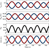 |
Fig. 7. QPE timing from the impact model. We show Trec, Papp, eapp, and the O–C diagrams for a nearly circular EMRI orbit with eccentricity e = 0.05, and parameters commensurate with those of GSN 069. Odd and even QPEs are shown in red and blue respectively. We point out that the data points in the lower panels (O–C diagrams) are not exactly aligned with those in the upper ones. This is because the abscissa of a given data point in O–C diagrams is a multiple of Ptrial rather than the observed QPE arrival time. |
The resulting Trec, Papp, and O–C diagrams are shown in the upper three panels of Fig. 8 for Pdisc = 44 d, while the lower panel only shows the O–C diagrams for Pdisc = 19 d. We chose to show Trec and Papp for the case of the longer modulating timescale not because we believe it to be a more plausible solution, but rather for visual clarity, as the different quantities are less compressed on the x-axis. The variability of all quantities depends on the interplay between the disc and the apsidal precession timescales, but disc precession dominates, breaking the anti-correlation pattern that is present when only apsidal precession is considered (see Fig. 7) and introducing instead correlated variability of Papp and O–C data. For both Pdisc, the simulated O–C diagrams shown in the two lower panels can be compared with the corresponding observed ones in Fig. 4 (as well as in Figs. B.1 and B.2). The two branches of the simulated O–C data are well correlated with minimal phase difference, and the modulating shape and period are in good agreement with the data for both the 44 d and 19 d disc precession periods. The modulation amplitude is somewhat under-estimated, but there is a good overall agreement. The modulation amplitude primarily depends on the disc misalignment idisc with respect to the z-axis. Although we did not explore the full parameter space as we are here interested in the general behaviour rather than in finding accurate best-fitting solutions and parameters, we nevertheless report that a good match with the observed ≃2.5 h modulation amplitude is reached by increasing idisc from 5° to ≃20°.
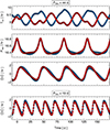 |
Fig. 8. Disc precession solution for GSN 069. In the upper three panels, we show Trec, Papp, and the O–C diagrams for a disc precession solution with Pdisc ∼ 44 d for GSN 069 (see text for further details). The lower panel shows the O–C diagrams for the same simulation but with Pdisc ∼ 19 d. |
The simulated O–C diagrams are not perfectly sinusoidal, which is visually more evident in the Pdisc = 44 d case, and this might actually be the origin of the ambiguity between the 43 d or ∼44 d modulation period in the odd and even QPEs data of GSN 069 since the latter was obtained by assuming a perfect sine function with sparse sampling. Trec and Papp shown in the two upper panels of Fig. 8 also comply with the requirements that are necessary for the model to represent a qualitatively viable solution to the QPE timing: the alternating recurrence times are preserved, but the perfect anti-correlation that is expected from the impact model with no disc precession is broken; the Papp for odd and even QPEs approximately align on a similar function, rather than being in phase opposition.
As mentioned, Franchini et al. (2023) have included disc precession in their impact model to reproduce single-epoch light curves of GSN 069, RX J1301.9+2747, eRO-QPE1, and eRO-QPE2. As noted in their work, the disc precession is much longer than that of the typical single-epoch observation (about 1.5 d), so that its effects on QPEs timing cannot be seen in their light curves. For GSN 069 they suggest a SMBH spin χ = 0.1 which, combined with a black hole mass of 106 M⊙, an EMRI semi-major axis of ≃160 Rg with orbital period Porb ≃ 18 h, and the assumed disc properties leads to Pdisc ≃ 125 d. Their modelling represents the first attempt to derive a self-consistent solution for the QPEs timing (as well as X-ray peak luminosity) including an external modulation, and can be considered successful at the qualitative level with the discrepancies (e.g. Pdisc ≃ 125 d instead or ≃19 d or ≃43–44 d) being likely only due to the limited baseline (single-epoch observations) used in their analysis.
We conclude that a rigidly precessing disc with precession period Pdisc = 19 d or 43–44 d represents a viable mechanism by which the impact model can be reconciled with the observed QPE timing data in GSN 069. It is also worth mentioning that, according to the study by Franchini et al. (2016), disc precession timescales of the order of ∼20–40 d can be reached for dimensionless black hole spin of the order of 0.1–0.6 for the relevant range of black hole masses. On the other hand, the disc precession timescale also depends on disc extent and structure (e.g. viscosity), so that deriving an estimate of the SMBH spin is not trivial.
9. Hierarchical triple: An outer SMBH binary and inner EMRI system
If the EMRI system we have considered so far was a member of a (hierarchical) triple system comprising an outer SMBH binary, orbital motion of the QPE-emitting inner EMRI around the centre of mass with the second SMBH would induce time delays in the time of arrivals of QPEs. Odd and even QPEs would be modulated in roughly the same way, as QPEs delays are simply associated with the light travel time from the impact to the observer, which is a function of the outer binary orbital phase and observer inclination. Within this scenario, Porb and Pmod in Table 1 are estimates of the inner, QPE-emitting EMRI orbital period, and the outer binary one respectively (Pout), while the amplitude of the O–C modulation (together with the observer inclination) sets the geometrical scale of the outer binary.
Since the O–C modulation in GSN 069 is consistent with a sine function, we assume for simplicity that the outer binary is on a circular orbit, although the sparse nature of the O–C data might allow for more complex functional forms associated with an eccentric outer binary. The orbital radius of the EMRI (or, equivalently of the SMBH with mass M1) around the centre of mass with M2 is then a1 = Amodc/sin iobs, where iobs is the angle between the observer line of sight and the outer binary angular momentum. a1 is related to the binary separation aout by aout = a1 (1 + q), where q = M1/M2 ≤ 1 and M2 is the outer SMBH mass. By using Kepler’s third law, one can then derive the total mass Mtot = M1 + M2 + m ≃ M1 + M2 as a function of Pmod, Amod, iobs, and q as
 (4)
(4)
Eq. (4) can then be used as a consistency check for the hierarchical triple hypothesis in GSN 069 by requiring that the Mtot derived by considering the observed upper limit on Pmod and lower limit on Amod does not exceed the upper limit from the M − σ relation. As mentioned, the uncertainties reported in Table 1 are statistical only, and our measurements are likely to be subject to some systematic uncertainty due to the unknown, and possibly impact-dependent, delays between impacts and QPE peak of emission. In the consistency check below, we then use as upper and lower limits on Pmod and Amod those obtained by assuming a 5% uncertainty on the best-fitting parameters whenever the statistical ones are smaller.
From the O–C analysis of GSN 069 (see Table 1), we derive two possible sets of Pmod and Amod. By inserting their upper and lower limits into Eq. (4), Mtot is consistent with the upper limit from the M − σ relation (∼3.2 × 10⁶ M⊙) if iobs ≳ 55° and q ≲ 0.2 for the ∼19 d modulation, and iobs ≳ 29° for any q ≤ 1 for the ∼43–44 d one. Hence, there is significant room for the presence of a SMBH binary in GSN 069 in both cases.
We have modified the numerical code presented in Franchini et al. (2023) introducing a second SMBH with mass M2 that forms, with the inner EMRI, a SMBH outer binary with orbital period Pout, and we computed the QPE times of arrival to assess whether a hierarchical triple system can account for the observed periodic modulation and correlation of the O–C diagrams in GSN 069 (see Appendix C for a description of the numerical implementation). We considered the cases of both a Pout = 44 d and 19 d assuming that the outer binary is responsible for the O–C modulation via light travel time effects. In both simulations, the outer SMBH binary orbit and the accretion disc around M1 were assumed to lie in the x-y plane, while iEMRI = 10° with respect to the z-axis. Our goal here was not to obtain an accurate fit to the data, but rather to investigate whether a SMBH outer binary could represent a viable qualitative solution for the observed QPE timing fulfilling the conditions outlined at the end of Section 6. Therefore, we did not vary the system geometry to search for a better quantitative agreement.
The first simulated system is composed by an inner, QPE-emitting EMRI with M1 = 8 × 10⁵ M⊙ (and m ≪ M1), eccentricity e = 0.05, and orbital period ∼18 h (see Table 1) and a second SMBH with M2 = 2 × 10⁶ M⊙. The total nuclear mass (ignoring the EMRI secondary) was then Mtot = 2.8 × 10⁶ M⊙, consistent with the range inferred from the M − σ relation in GSN 069 (see Section 7). The outer binary was set on a circular orbit with orbital period Pout = 44 d. The observer inclination was set to iobs = 60°. The resulting outer SMBH binary semi-major axis is ∼1.67 × 10⁻⁴ pc, and the triplet is stable with a merger time of ∼0.1 Myr for the outer SMBH binary. The second simulation was realised with M1 = 2.2 × 10⁵ M⊙, M2 = 2.8 × 10⁶ M⊙, Pout = 19 d, and iobs = 75°. The resulting outer SMBH binary semi-major axis is ∼9.8 × 10⁻⁵ pc, and the triplet is stable with a relatively short merger time of ∼2.8 × 10⁴ yr for the outer SMBH binary.
In the upper three panels of Fig. 9, we show the resulting Trec, Papp, and O–C diagrams for Pout = 44 d while, in the lower panel, we only show the O–C diagrams for Pout = 19 d. The simulated quantities satisfy all properties outlined at the end of Section 6, and thus qualify as a viable solution for the QPE timing behaviour of GSN 069: the alternating recurrence times are preserved, but the two branches are not exactly anti-correlated allowing, for instance, for time intervals in which the drop (rise) in one branch is more pronounced than the rise (drop) in the other, as observed in Fig. 3. The odd and even branches in both Papp and the O–C diagrams are well correlated, roughly in phase, and periodic at the outer binary orbital period Pout. In particular, the simulated O–C diagrams (two lower panels in Fig. 9) can be compared to the corresponding observed ones in Fig. 4 as well as with those associated with different QPE identifications in Figs. B.1 and B.2. The agreement between the observed and simulated O–C diagrams in timescale, shape, and modulating amplitude is excellent.
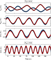 |
Fig. 9. Hierarchical triple solution for GSN 069. In the upper three panels we show Trec, Papp, and the O–C diagrams for a hierarchical triple solution for GSN 069 comprising the inner, QPE-emitting EMRI and an outer circular SMBH binary with orbital period Pout = 44 d. The O–C diagrams for the alternative solution with Pout = 19 d are shown in the lower panel. |
We conclude that a hierarchical triple system composed by the inner, QPE-emitting EMRI and an outer SMBH binary with sub-milliparsec separation is a viable solution that can account for the observed periodicity and correlation of the O–C diagrams for odd and even QPEs while preserving the alternating recurrence times and aligning the orbital timescale Papp for the two branches on the same functional form.
10. Quiescent X-ray emission modulation
In principle, both the disc precession and hierarchical triple scenarios outlined above might induce a modulation of the quiescent (out-of-QPEs) X-ray disc emission in GSN 069 on the same timescale over which the O–C diagrams are modulated. The variability of the quiescent X-ray emission in GSN 069 can thus be used to confirm the external modulation scenario suggested by the O–C analysis, and perhaps even to constrain its origin.
Disc precession generally modulates the disc emission on the precession timescale, but it is not necessarily associated with an X-ray modulation. This is because, the modulation probed via the O–C analysis is associated with delayed or anticipated QPEs that are produced by the impacts between the EMRI’s secondary and the disc. Such impacts occur on a ring on the disc whose inner and outer boundaries are set by the pericentre and apocentre distances of the EMRI orbit, namely, a (1 ± e) where a and e are the orbit semi-major axis and eccentricity. Given the assumed parameters in GSN 069 (Porb ≃ 18 h, eorb ≃ 0.05, and M = 8 × 10⁵ M⊙), impacts occur on a ring at 180–200 Rg from the centre. This portion of the disc is significantly farther away than the X-ray emitting region (likely few tens of Rg only), and it is instead associated with UV or optical disc emission, so that the disc precession model predicts periodic variability at these longer wavelengths. This is currently difficult to probe due to stellar contamination in the galactic nucleus and monitoring Hubble Space Telescope observations over a tens of days baseline are needed to explore this possibility.
X-ray periodic variability of the quiescent disc emission is only expected if the disc precesses rigidly so that the inner X-ray emitting disc also precesses on the same timescale. This is not granted, as the disc might not fulfil the conditions for rigid precession (Franchini et al. 2016), or might break or tear into rings precessing on their own timescale. The precessing disc is bound to align with time on a timescale that can be of the order of years for relatively low black hole mass and effective viscosity values, so that observing a precessing disc in GSN 069 years after the TDE-like outburst is possible (Franchini et al. 2016). Moreover, if rigid disc precession holds, viscous spreading of the disc with time leads to an increase of the disc precession timescale during alignment (Teboul & Metzger 2023), a prediction that might be tested if the quiescent X-ray emission is indeed modulated. As mentioned in Section 8, a good match with the O–C modulation amplitude is obtained for a disc misalignment of the order of 20°. The predicted X-ray flux modulation is however also a function of the observer inclination iobs. Since iobs has a minor effect on O–C data, we could not constrain it, and the expected X-ray flux modulation amplitude in the case of (rigid) disc precession spans a wide range that corresponds to the different possible lines-of-sight.
In the case of a triple system (the inner binary containing the EMRI and an outer SMBH), orbital motion of the EMRI system about the centre of mass does not only modulate QPEs times of arrival, but also the X-ray emission from the inner regions of the accretion disc via Doppler boosting. Assuming that the emitted radiation has spectrum F ∝ να in frequency space, and for orbital velocities βorb = vorb/c ≪ 1, the fractional variability due to Doppler boosting from the motion within a circular binary can be written as
 (5)
(5)
where ϕorb is the orbital phase, and iobs is the observer inclination (Loeb & Gaudi 2003; D’Orazio et al. 2015; Charisi et al. 2018).
However, as discussed in Section 9, when interpreting the O–C modulation in terms of time delays due to orbital motion in an SMBH binary, the O–C modulation amplitude Amod sets the radius of the orbit of the EMRI system around the centre of mass with the outer SMBH as R = Amodc/sin iobs, while the period of the O–C modulation (Pmod) is assumed to match the SMBH binary orbital period, i.e. Pmod = Pout. Therefore, the orbital velocity is simply
 (6)
(6)
By inserting the orbital velocity into Eq. (5), we obtain
 (7)
(7)
that can be used to estimate the predicted modulation semi-amplitude, reached for cos ϕorb = 1 corresponding to the orbital phase when the X-ray emitting disc (and the EMRI binary) are on the approaching side of the outer binary orbit. By considering that the thermal SED of GSN 069 has typical spectral index α ≃ −9 in the 0.3–1 keV band, and inserting the numbers for Amod and Pmod obtained from the O–C analysis, the fractional variability semi-amplitudes in the 0.3–1 keV X-ray band is then
 (8)
(8)
where we have assumed the mean Amod and Pmod from Table 1 for the two possible periods. Naturally, the shortest period corresponds to the highest-amplitude modulation since the orbital velocity is the highest, thus maximising the effect of the Doppler boost. Hence, if the O–C modulation is due to light-travel-time effects in an outer SMBH binary, the Doppler boosting model predicts the X-ray flux variability amplitude with no free parameters, as the amplitude only depends on measured quantities (spectral index α, and the amplitude Amod and period Pmod of the O–C modulation). This clear prediction can then be tested against monitoring X-ray data.
GSN 069 was monitored on several occasions in the X-rays precisely in the attempt to search for a periodic modulation of the quiescent disc emission. However, the quiescent X-ray variability on both short and long timescales had typically an amplitude well above the 50% level, which prevented us from looking for relatively low-amplitude modulations (results will be presented elsewhere). Swift and NICER are currently monitoring GSN 069 over an extended baseline, and the source has apparently entered a period of high average flux and relatively low-amplitude X-ray variability since May 2024. We note that, consistent with the QPE disappearance at high fluxes reported by Miniutti et al. (2023b), no QPEs have been detected so far in the on-going campaign since May 2024 which also comprises a long-enough ∼120 ks XMM-Newton observation that failed to detect any clear QPE.
The current X-ray light curve from Swift and NICER is shown in Fig. 10. In both cases, the light curves have been normalised to the respective best-fitting constant model during the campaign to remove calibration uncertainties between detectors, and to ease comparison as we are here interested in fractional variability amplitudes. The Swift XRT typically collects few to few tens of counts per observation so that no spectral information is available. Hence, the data points in Fig. 10 represent the normalised 0.3–1 keV count rate. Any two consecutive Swift observations delivering consistent count rates have been combined to improve the signal-to-noise. On the other hand, each NICER data point comprises a series of snapshot exposures with typical duration of few hundred seconds. We have analysed the X-ray spectra of each individual snapshot exposure5, and the resulting X-ray flux from exposures within a few hours has then been combined. Each NICER data point in Fig. 10 represents the average 0.3–1 keV X-ray flux (and standard deviation) from exposures within a few hours, normalised to the best-fitting constant model throughout the NICER campaign.
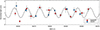 |
Fig. 10. 2024 Swift and NICER monitoring campaign. We show the normalised 0.3–1 keV quiescent light curves of GSN 069 as obtained by the Swift XRT and by NICER during the current campaign. Any two consecutive Swift observations with consistent count rates have been combined to reduce the statistical uncertainty. Individual NICER snapshots have been analysed separately, and the data points represent the mean 0.3–1 keV flux and standard deviation obtained within a few hours. The dashed line is a sine function modulation with period ≃19.9 d and semi-amplitude ≃45% resulting in χ2 = 31 for 17 degrees of freedom. |
A constant model fit to the combined Swift and NICER data sets shown in Fig. 10 results in χ2 = 95.0 for 20 degrees of freedom. In order to search for possible modulations, we added a sinusoidal function (three free parameters) to the model which resulted χ2 = 31 for 17 degrees of freedom, i.e. an improvement that is statistically significant at the ∼99.98% level from a simple F-test. The corresponding, best-fitting sinusoidal modulation is shown as dashed line in Fig. 10. Although the statistical improvement obtained by adding the sinusoidal modulation to a constant model is formally high, the number of cycles is still too small to draw firm conclusions about the presence of the X-ray modulation, considering also the sparse sampling in Fig. 10.
The best fitting period and semi-amplitude are P = 19.9 ± 0.3 d and A = 0.45 ± 0.06. The modulating period is therefore consistent, within 3–4%, with the ∼19 d modulation inferred from the completely independent technique of O–C diagrams, which is based exclusively on QPEs times of arrival, while the (tentative) flux modulation from the Swift and NICER data is obtained from out-of-QPEs quiescent flux variability. Remarkably, the variability amplitude is consistent with that predicted from Doppler boosting for the ∼19 d period (≃42%, see Eq. (8)). In the case of a rigidly precessing disc, the 40–50% modulation suggested by the Swift and NICER data can be reproduced by various combinations of disc misalignment and observer inclination although, for consistency with the O–C modulating amplitude, a disc misalignment of the order of 20° appears favoured (see Section 8).
In the upper panel Fig. 11, we show the normalised light curve folded at the best-fitting period of 19.9 d with the sinusoidal best-fitting modulation over-plotted to guide the eye as a solid line (dotted lines represent the 1σ range of allowed amplitude). In the lower panel, we show the same data together with the expected Doppler boosting modulation (blue), and one realisation of the disc precession induced modulation in which we consider a disc misaligned by 20° with respect to the SMBH’s spin (consistent with the O–C modulation), and an intermediate observer inclination of 45°.
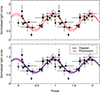 |
Fig. 11. Folded Swift and NICER light curve. The upper panel shows the light curve of Fig. 10 folded at the best-fitting period of 19.9 d. Two cycles are shown for visual clarity, and the distinction between Swift and NICER data points has been removed. The solid red line represents the sinusoidal modulation with 1σ uncertainties in its amplitude shown as dotted lines. In the lower panel, we show the predicted modulation from Doppler boosting (blue) as well as one possible realisation of the disc precession model (red) corresponding to a disc misalignment of idisc = 20° and observer inclination iobs = 45°. |
However, a series of eight XMM-Newton observations obtained between MJD 60 482 and 60 510 do not fully confirm the modulation tentatively seen with Swift and NICER. Only a few (three or four) XMM-Newton observation show quiescent 0.3–1 keV fluxes roughly consistent with the modulation shown in Fig. 10, while others have lower-than-predicted flux level by a significant amount. This is shown in Fig. 12 where we reproduce the light curve of Fig. 10 in a restricted range and included the normalised 0.3–1 keV flux resulting from spectral analysis of the XMM-Newton EPIC-pn camera’s data (see Appendix A for details). The discrepancies between the XMM-Newton data and the sinusoidal modulation suggested by the Swift and NICER monitoring casts some doubts on the reality of the quiescent flux periodicity, and only further higher cadence, monitoring observations on a longer baseline can provide a firm result, clarifying whether the discrepant XMM-Newton data points can be attributed to occasional intrinsic variability.
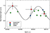 |
Fig. 12. Zoom of Fig. 10 over a restricted MJD range in which eight XMM-Newton observations are also available (green crosses). The XMM-Newton data points show the 0.3–1 keV average X-ray flux during each XMM-Newton observation, normalised to the best-fitting constant model over the spanned baseline. Uncertainties on the XMM-Newton data are included, but smaller than symbol size. |
We are continuing to monitor GSN 069 with Swift every few days, and we have significantly increased the cadence of the NICER observations. The combined monitoring will enable us to assess the statistical significance of any modulation on firmer statistical grounds than possible at present. Having monitored the source also in the past, we must stress that there is no guarantee that the current relatively low-amplitude variability continues in the future. Past data show that the X-ray flux enters phases or relatively low intrinsic variability that are reminiscent of sinusoidal behaviour similar to that shown in Fig. 10, but these phases are often interrupted by periods of enhanced variability during which it is difficult, if not impossible, to search for lower-amplitude modulations. At this stage, we refrain from providing possible explanations for the observed discrepancy between the XMM-Newton and the Swift and NICER measurements as they would represent mere speculations. Future monitoring data are the only reliable way of assessing whether the quiescent disc emission in GSN 069 is indeed modulated periodically.
11. Discussion
Within the context of the impact model for QPEs, a consistent picture is starting to emerge from observations. The data are consistent so far with pre-existing EMRI systems that are revealed electromagnetically through QPEs whenever an accretion disc extending further than the secondary orbit is present. Interactions between the disc and the orbiting secondary produce the observed high-amplitude quasi-periodic flares. The association between QPEs and TDEs, first suggested in the case of GSN 069 (Shu et al. 2018; Miniutti et al. 2019) and then strengthened by the detection of QPEs in two optically-selected TDEs (Quintin et al. 2023; Nicholl et al. 2024) among other evidences, indicates that the accretion disc is likely the result of the full or partial tidal disruption of a star by an otherwise inactive SMBH. Such a disc is initially compact, with outer radius of the order of few times the tidal radius (typically tens of Rg), and could be smaller than the typical EMRI orbit. As the accretion disc spreads out viscously, it intercepts the EMRI orbit and gives rise to the start of the QPE phenomenon. QPEs are therefore generally expected to only appear at late times, with a delay with respect to the TDE peak. On the other hand, if the tidally disrupted star is evolved, as might be the case in GSN 069 (Sheng et al. 2021), its tidal radius can be of the order of hundreds of Rg, so that QPEs due to EMRI orbits with semi-major axis of 100–200 Rg may have started immediately. In GSN 069, a sufficiently long X-ray observation ∼4.5 yr after the initial X-ray outburst failed to detect any QPEs. These were first detected in December 2018, about 8.5 yr after the X-ray peak. Hence, QPEs in GSN 069 appeared with a delay of ∼4.5–8.5 yr with respect to the initial TDE-like outburst, which may be taken as an indication of a delayed QPE appearance. However, later observations have shown that QPEs disappear above a given X-ray luminosity (or mass accretion rate) threshold which may be the reason why no QPEs were detected during the sufficiently long but high flux observation ∼4.5 yr after TDE peak (Miniutti et al. 2023b).
11.1. QPE timing properties: disc precession or a SMBH binary
The impact model for QPEs, in which the secondary EMRI component pierces through a non-precessing accretion disc around the primary, produces alternating recurrence times for any non-zero orbital eccentricity, in good agreement with the observed QPE timing properties in GSN 069 and other QPE sources. Such a model also naturally implies that odd and even QPEs share a common baseline period (and period derivative, if present), as this is set by the EMRI orbital properties and evolution. However, when no external modulation is included, the model predicts that recurrence times Trec (separation between consecutive QPEs), apparent orbital period Papp (separation between consecutive QPEs of the same parity), and O–C diagrams for odd and even QPEs are periodic on the (super-orbital) apsidal precession timescale and, most importantly, are all in phase opposition. In absence of an external modulation that is faster than apsidal precession and of sufficiently high amplitude to dominate the timing, these are unavoidable consequences of relativistic orbits dynamics.
None of the three observed quantities in GSN 069 appear to comply with this very clear expectation. In particular, the O–C diagrams are consistent with being periodic on a super-orbital timescale of the order of tens of days, but odd and even QPEs data are well correlated with a minimal phase difference (actually simply due to the fact that odd and even QPEs are not simultaneous but separated by Trec), contrary to model’s predictions. Also, the amplitude of the O–C modulation is about one order of magnitude higher than that expected from apsidal precession alone, given the modest EMRI’s eccentricity inferred in GSN 069 (≲0.15). On the other hand, our O–C analysis shows that solutions in which odd and even QPEs share a common period (and, if present, period derivative) do exist, which is fully consistent with the impact scenario, and suggests that the model might need to be modified rather than rejected.
The observed modulation of the O–C diagrams in GSN 069 is likely associated with an external physical mechanism unrelated to the EMRI orbital properties (see also Chakraborty et al. 2024). We have explored two possible sources of modulation: disc precession and light-travel-time effects due to the motion of the QPE-emitting system (EMRI plus disc) around the centre of mass of an outer SMBH binary system. Both mechanisms qualitatively reproduce the correlated modulation (with period Pmod) of the O–C diagrams for odd and even QPEs, where Pmod is set by the disc precession timescale or the outer SMBH binary orbital period. Fig. D.1 illustrates the effects on O–C diagrams (or QPEs time delays with respect to a given reference) of the various processes considered in this work.
As shown in Figs. 8 and 9, the two driving mechanisms produce almost identical O–C diagrams, so that this technique is not very useful to pinpoint the modulating physical process at play. However, the two scenarios can be easily distinguished from the shape of Papp (that is the time intervals between consecutive QPEs of the same parity) over at least one cycle. In the case of disc precession, Papp exhibits distinctive peaks6 repeating every disc precession period and separated by intervals of nearly constant behaviour. On the other hand, in the case of a hierarchical triple system, the Papp evolution is sinusoidal-like with period equal to that of the outer binary (see Figs. 8 and 9). A sufficiently dense X-ray monitoring campaign over at least one cycle in which the individual continuous exposure is long enough to detect at least three consecutive QPEs will enable us to accurately measure the shape of Papp, and therefore to distinguish between the two proposed scenarios.
Another possible way of distinguishing between the two physical processes is through a new O–C campaign on GSN 069. In the case of a SMBH binary, the modulating period decay must be consistent with that from GW emission. Assuming fiducial parameters for a circular SMBH binary with total mass of 3 × 10⁶, mass ratio q = 0.1, and orbital period of ≃19 d (similar to that providing a good match with the data), the GW period derivative is ṖGW ≃ 8.3 × 10⁻⁷ or ∼3 × 10⁻⁴ d per year, which is undetectable in the X-rays even on a 10 or 20 yr baseline. The same is true for the modulating amplitude because the outer SMBH binary orbit does not harden sufficiently fast to lead to detectable amplitude decay. In the case of disc precession, the disc precession timescale is expected to be longer in the future as the disc extends farther out due to viscous spreading. Moreover, as the disc alignment process continues, the modulating amplitude is also expected to decay on months or years timescales (Teboul & Metzger 2023). A new O–C campaign detecting a longer modulating period with lower amplitude would therefore favour the disc precession model and rule out the SMBH binary one.
11.2. Hints for period decay in GSN 069 and possible interpretations
The ambiguity on QPE’s identification during the May 2019 observation of GSN 069 implies that the EMRI orbital period Porb might be decaying. The O–C data are consistent with three possible solutions for the period derivative, namely Ṗorb = 0, −3–4 × 10⁻⁵, or −6–7 × 10⁻⁵. An hint for a period decay of Ṗorb ≃ −3–4 × 10⁻⁵, consistent with the O–C solutions discussed in Section 4.1, is obtained by comparing Porb, as derived from the O–C data between December 2018 and May 2019, with the average Papp (a proxy for the actual Porb) in a June–July 2023 campaign. This estimate cannot be considered as a secure detection because it is only based on the average Papp in 2023, which may significantly underestimate the actual EMRI orbital period due to the restricted number of independent measurements in 2023. However, with the caveat that the detection of such a  is tentative only, we discuss its possible implications in some more detail.
One obvious source of period decay in an EMRI system is gravitational wave (GW) emission. However, if the EMRI secondary is a star rather than a black hole, hydrodynamical drag from repeated star-disc collisions naturally induces a (negative) period derivative as well (for relevant formulae, see e.g. Linial & Metzger 2023; Linial & Quataert 2024; Arcodia et al. 2024b). Assuming that the tentative Ṗorb is only due to GW emission, its amplitude together with the derived EMRI orbital period and eccentricity implies that, even for a primary black hole mass at the high end of the range allowed from the M − σ relation (≃3.2 × 10⁶ M⊙), the secondary mass needs to be m ≳ 105 M⊙ effectively defining a SMBH binary rather than an EMRI (semantically defined as a binary with mass ratio q ≤ 10−4).
If the period decay is instead due to hydrodynamical gas drag,  where R⋆ and m⋆ are the radius and mass of the orbiting star and Σ is the disc surface density (Linial & Quataert 2024; Arcodia et al. 2024b). For a Sun-like star that does not change structure due to collisions, a relatively high Σ ≳ 106 g cm−2 at the impact site would be required to match the observed period decay in GSN 069. Considering fiducial parameters for GSN 069 (a non-spinning SMBH with mass of 8 × 10⁵ M⊙, secondary orbital period of 18 h, and an average impact radius of ≃190 Rg) and assuming a surface density radial profile Σ = Σ0(R/Rg)−p with p = 3/5, the condition Σ ≳ 106 g cm−2 at impact implies an overall accretion disc mass Mdisc ≳ 1.2 M⊙ for a disc extending out to ≈200 Rg, the minimum outer radius that allows for two impacts per orbit7.
We point out, however, that the repeated collisions between the star and the disc would generally result in the inflation of the star’s outer layers (Yao et al. 2025). Since, in the hydrodynamical gas drag scenario, the disc surface density scales as  , a lighter star whose radius was inflated above the equivalent main-sequence value would result in a lower inferred Σ, possibly down to ∼104 g cm−2 at the collisions site, thus leading to a significantly lower minimum disc mass. As mentioned in Section 4.1, other mechanisms related to longer-term modulations (e.g. nodal precession of the EMRI orbital plane in case of a Kerr primary SMBH) might give rise to apparent Ṗorb≠ 0 or, at least, to more complex behaviour as discussed, for instance, by Arcodia et al. (2024b). This suggests that the tentative Ṗorb we report should not be over-interpreted.
11.3. Modulation of the quiescent disc emission
As discussed in Section 10, Swift and NICER monitoring observations from May to September 2024 indicate a possible modulation of the X-ray disc emission in GSN 069 with a period of ∼19.9 d and semi-amplitude of 40–50%. The period is formally slightly longer than the ∼19 d solution of the O–C analysis from QPEs times of arrival but consistent with it within a few per cent which, considering the likely systematic uncertainties affecting the O–C results, suggests not to claim a statistically significant difference at this stage. The relatively small number of observed cycles, sparse sampling, and some discrepant XMM-Newton data points, suggest to consider the X-ray flux modulation as tentative only. Nevertheless, it is encouraging that the tentative period is broadly consistent with the O–C solution associated with the ∼19 d modulation, as the two analysis are completely independent from one another, which provides some support to the robustness of both.
Disc precession can be associated with a wide range of possible modulating amplitudes, depending on the actual disc misalignment with respect to the SMBH spin axis (here simply the z-axis) and on observer inclination. A good match with the O–C modulation amplitude of ∼2.5 h is reached for a disc misalignment of ≃20° with respect to the z-axis. Assuming this misalignment, the quiescent X-ray flux modulation is consistent with intermediate observer inclinations of the order of 45°.
In the case of Doppler boosting of the inner disc emission in an outer SMBH binary, the predicted variability amplitude has no free parameters once a solution for the O–C analysis is selected (with either Pmod ≃ 19 d or ≃43–44 d). This is because, if the O–C diagrams modulation is interpreted within this context, the orbital velocity is set by the orbit’s size and period, that are measured through Amod and Pmod modulo the sine of observer inclination, which however cancels out in Eq. (5). Considering the observed steep X-ray spectrum, Doppler boosting predicts a relatively precise ∼42% variability amplitude for the ∼19 d O–C modulation, which is indeed consistent with the observed quiescent X-ray flux modulation of 40–50%.
As discussed in Section 11.1, the two scenarios make different predictions on the modulating period and amplitude time evolution, with only the disc precession model giving rise to detectable changes. Future monitoring observations able to follow the quiescent flux evolution in terms of both period and amplitude might then unveil the actual modulating process. As a further note, we point out that, in the SMBH binary scenario, QPEs time delays reach their maximum and minimum value at orbital phases corresponding to the far and near sides of the outer SMBH binary orbit with respect to the observer, while the extremes of the disc X-ray emission by Doppler boosting are expected at phases corresponding to the approaching and receding sides. A phase shift of 1/4 Pout between the O–C delays and the X-ray flux variability is therefore expected. Detecting the Doppler-induced modulation of the X-ray flux at the correct phase with respect to O–C time delays would represent a smoking gun for the presence of a tight SMBH binary in the nucleus of GSN 069. This is not presently possible as the 2018–2019 observations (from which we derive QPEs delays) and the 2024 monitoring campaign are too far apart to be aligned considering the current period uncertainty of few per cent. However, future campaigns in which a sufficiently large number of QPEs are obtained quasi-simultaneously with quiescent X-ray fluxes on a few days cadence might prove key in this respect.
12. Summary and conclusions
We have studied the QPEs timing properties in GSN 069 primarily using X-ray data from three XMM-Newton and one Chandra observations between December 2018 and May 2019. These data were complemented by three XMM-Newton observations in 2023, and by a series of XMM-Newton, Swift, and NICER monitoring observations between May and September 2024. Our primary goal was to compare the observed QPEs timing properties with predictions from one of the most popular models for QPEs, that of a secondary orbiting body piercing through the accretion disc around a primary SMBH in an EMRI system, with each impact producing one QPE. The main conclusions of our study are summarised below.
In 2018–2019, and with the caveats discussed in Section 4.1, the O–C diagrams for odd and even QPEs are consistent with a periodic modulation on a timescale of either ≃19 d or ≃43–44 d with semi-amplitude of ≃2.5–2.8 h. The sparse nature of the data prevents to distinguish between the two possible periods. The O–C data provide a measurement of the EMRI orbital period (Porb ≃ 18 h) and are consistent with either no orbital evolution (Ṗorb = 0), or with period derivatives Ṗorb ≃ −3–4 × 10⁻⁵ or Ṗorb ≃ −6–7 × 10⁻⁵, the intermediate value being supported by the estimated orbital period during a 2023 campaign, although we point out that an apparent period derivative might be induced by longer-timescale modulations that are currently out of observational reach (see e.g. Fig. C.1 for the case of orbital nodal precession induced by the SMBH spin).
The O–C diagrams for odd and even QPEs have minimal phase differences (given by the average recurrence time between consecutive QPEs, ∼9 h or ∼0.38 d). This is contrary to the expectations from the impact model with no external modulation as O–C data for odd and even QPEs are predicted to be periodic on the apsidal precession timescale and in phase opposition, an unavoidable consequence of relativistic orbits dynamics. Moreover, the observed O–C modulating amplitude is about one order of magnitude higher than that expected from apsidal precession alone.
For the impact model to apply, an external modulation, unrelated to the EMRI’s orbit, needs to be considered. Through numerical simulations of impact times between the secondary and the disc, we show that a rigidly precessing accretion disc or an outer SMBH (forming with the inner QPE-emitting EMRI a sub-milliparsec SMBH binary) qualitatively describe the QPEs timing data, reconciling the observed properties with the impact model. Both models qualify as a qualitative solution for the QPE timing behaviour: they both preserve the alternating recurrence times while producing an evolution in which odd and even QPEs Trec are not in phase opposition; they align the apparent orbital period Papp for the two branches on the same (or similar) function; additionally, they produce O–C diagrams that are periodic on a super-orbital timescale (the disc precession or the outer SMBH orbital one) with minimal phase difference, rather than being in phase opposition.
We report evidence to support a periodic modulation of the quiescent X-ray (disc) flux in GSN 069 during a 2024 monitoring campaign with period ≃19.9 d and semi-amplitude of ≃40–50%, although the relatively small number of cycles so far, as well as some discrepant data points suggest to consider the periodicity as tentative until (and if) further cycles are accumulated. The inferred period is consistent, within a few per cent, with the O–C analysis ∼5 yr earlier for the case of the ≃19 d modulation. We point out that the two modulations are obtained from completely independent data and techniques supporting each other’s robustness. Both scenarios proposed to explain the O–C modulation (disc precession and a SMBH binary) are consistent with the flux modulation amplitude. In fact, the SMBH binary model, in combination with results from the O–C analysis, predicts a flux variability of 42%, of the order of that tentatively observed, with no free parameters. Disc precession is consistent with the variability amplitude for a broad range of the two driving parameters, the disc’s angular momentum misalignment and the observer inclination. A disc misalignment of ≃20°, resulting in an O–C modulation amplitude consistent with the observed one, produces the observed X-ray flux modulation amplitude for intermediate observer inclination of ∼45°. The evolution of the flux modulation in both period and amplitude might constrain the origin of the external modulation in the future, as the period is expected to increase (and the amplitude to decrease) only in the case of disc precession.
Both scenarios proposed here, disc precession or the presence of a SMBH binary, are plausible in TDEs and, given the mounting evidence that QPEs systems reside in TDEs, in QPE systems. As the tidally disrupted star approaches the SMBH from a random direction, the bound debris will generally form a misaligned accretion disc with respect to the SMBH spin axis. As a result, disc precession is likely to take place initially, and could imprint multi-wavelength variability signatures (Stone & Loeb 2012; Pasham et al. 2024b). If the disc is precessing rigidly, the innermost accretion disc emission is also modulated at the global disc precession timescale which depends on SMBH’s mass and spin, but also on disc extent and structure. The alignment timescale depends on SMBH’s and disc’s properties, and it might last long enough to still be observable years after the TDE as would be the case in GSN 069 (Franchini et al. 2016). On the other hand, the presence of a nuclear SMBH binary significantly enhances TDE rates in galactic nuclei due to the combined effect of the Kozai-Lidov secular mechanism (Kozai 1962; Lidov 1962) and to resonant interactions of stars with the secondary black hole (Ivanov et al. 2005; Chen et al. 2011); thus finding SMBH binary candidates in TDEs is somewhat expected. In GSN 069, for stability reasons in a triple system, the EMRI plus disc QPE-emitting system needs to be associated with the lighter SMBH whose mass ratio with the more massive member of the SMBH binary is of the order of q ≲ 0.2. Assuming, for example, the (non-unique) parameters that provide a good match to the O–C data for the ∼19 d solution, that is, Mtot ≃ 3.02 × 10⁶ M⊙, q ≃ 0.079, and Pout = 19 d, the outer binary has a separation of ≃9.8 × 10⁻⁵ pc or ≃730 Rg (where the gravitational radius is that of the more massive SMBH). It will then merge in a relatively short time of the order of 2.8 × 10⁴ yr.
Future X-ray monitoring observations, if appropriately designed, can be used to confirm (or reject) the overall impact-plus-external-modulation model as well as the reality of the quiescent (disc) X-ray flux periodicity. For the latter case, the on-going Swift and NICER campaign has been extended, which should be sufficient to confirm the quiescent X-ray flux modulation (if present) within a few months. Moreover, future observations will enable us to distinguish between the two proposed scenarios by comparing their (different) predictions on QPEs timing and disc variability. Complementing such X-ray observations with high spatial-resolution monitoring observation in the optical and UV with the Hubble Space Telescope will also be important as the Doppler boosting and precession models make distinct predictions on the quiescent disc variability amplitude as a function of wavelength. Moreover, if the weak radio flux in GSN 069, ≃47 μJy at ∼6 GHz (Miniutti et al. 2019), is associated with a compact jet, high-cadence radio observations with sufficient sensitivity might reveal variability consistent with orbital motion or a precessing jet.
If the impact-plus-modulation model is indeed correct, the X-ray QPEs detected in December 2018 in GSN 069 represent the first electromagnetic detection of an extragalactic, short-period EMRI system. This detection potentially paves the way to future electromagnetic and gravitational wave synergies and multi-messenger astronomy. As shown here, the QPEs properties and timing encode unique information of the likely complex galactic nuclei and SMBH inner environment, which can improve our understanding of the structure and dynamics of accretion flows around recently activated SMBHs. It may also possibly contribute to reveal the presence of hierarchical triples and tight, sub-milliparsec SMBH binaries in galactic nuclei.
While Franchini et al. (2023) considered a precessing accretion disc, this was not included in the work by Zhou et al. (2024b).
In absence of disc or nodal precession, the only relevant angle is that between the disc and the EMRI’s orbit angular momenta, so having a disc inclined with respect to the equatorial plane is not necessary here. However, the same set-up will be used in Section 8 when discussing the effects of disc precession, so that we introduce the adopted geometry here.
If the modulation had longer timescale than apsidal precession, it will produce a correlation on long timescales, but the anti-correlation on short ones would remain, exactly as is the case for the modulation induced by the orbital nodal precession shown in Fig. C.1.
This is necessary to account for the variable NICER background, see Appendix A for details.
Note than if the disc and EMRI’s orbit angular momenta do not have the same sign (with respect to the SMBH spin), the peaks in Papp revert into valleys.
Note that Franchini et al. (2023) assumed a 4 M⊙ disc for GSN 069 when reproducing single-epoch QPE light curves with their impacts plus disc precession model.
Acknowledgments
GM thanks Ari Laor for many valuable discussions on O–C data interpretation and Eric Agol for suggesting to use O–C diagrams in QPEs data analysis years ago. We also thank Chris Done for providing a version of the optxagnf model including retrograde accretion (negative black hole spin). We thank the XMM-Newton, Chandra, Swift, and NICER teams for their excellent work and continued support. This work is based on observations obtained with XMM-Newton, an ESA science mission with instruments and contributions directly funded by ESA Member States and NASA. We also used data obtained from the Chandra X-ray mission, and software provided by the Chandra X-ray Center (CXC). We acknowledge the use of public data from the Neil Gehrels Swift Observatory data archive. This work made use of data supplied by the UK Swift Science Data Centre at the University of Leicester. We acknowledge the use of data and software provided by the High Energy Astrophysics Science Archive Research Center (HEASARC), which is a service of the Astrophysics Science Division at NASA/GSFC. GM acknowledges support by grant PID2020-115325GB-C31 funded by MCIN/AEI/10.13039/50110001103. AF acknowledges support provided by the “GW-learn” grant agreement CRSII5 213497 and the Tomalla Foundation. MB acknowledges support provided by MUR under grant “PNRR – Missione 4 Istruzione e Ricerca – Componente 2 Dalla Ricerca all’Impresa – Investimento 1.2 Finanziamento di progetti presentati da giovani ricercatori ID:SOE_0163” and by University of Milano-Bicocca under grant “2022-NAZ-0482/B”. MG is supported by the “Programa de Atracción de Talento” of the Comunidad de Madrid, grant number 2022-5A/TIC-24235, and by Spanish MICIU/AEI/10.13039/501100011033 grant PID2019-107061GB-C61. RA was supported by NASA through the NASA Hubble Fellowship grant n. HST-HF2-51499.001-A awarded by the Space Telescope Science Institute, which is operated by the Association of Universities for Research in Astronomy, Incorporated, under NASA contract NAS5-26555. Support for this work was provided by NASA through the NASA Hubble Fellowship grant HST-HF2-51534.001-A awarded by the Space Telescope Science Institute, which is operated by the Association of Universities for Research in Astronomy, Incorporated, under NASA contract NAS5-26555. IL acknowledges support from a Rothschild Fellowship and The Gruber Foundation, as well as Simons Investigator grant 827103. AS acknowledges the financial support provided under the European Union’s H2020 ERC Consolidator Grant “Binary Massive Black Hole Astrophysics” (B Massive, Grant Agreement: 818691).
References
- Amaro-Seoane, P., Audley, H., Babak, S., et al. 2017, ArXiv e-prints [arXiv:1702.00786] [Google Scholar]
- Arcodia, R., Merloni, A., Nandra, K., et al. 2021, Nature, 592, 704 [NASA ADS] [CrossRef] [Google Scholar]
- Arcodia, R., Miniutti, G., Ponti, G., et al. 2022, A&A, 662, A49 [NASA ADS] [CrossRef] [EDP Sciences] [Google Scholar]
- Arcodia, R., Liu, Z., Merloni, A., et al. 2024a, A&A, 684, A64 [NASA ADS] [CrossRef] [EDP Sciences] [Google Scholar]
- Arcodia, R., Linial, I., Miniutti, G., et al. 2024b, A&A, 690, A80 [NASA ADS] [CrossRef] [EDP Sciences] [Google Scholar]
- Arnaud, K. A. 1996, ASP Conf. Ser., 101, 17 [Google Scholar]
- Babak, S., Gair, J., Sesana, A., et al. 2017, Phys. Rev. D, 95, 103012 [NASA ADS] [CrossRef] [Google Scholar]
- Bandopadhyay, A., Coughlin, E. R., Nixon, C. J., & Pasham, D. R. 2024a, ApJ, 974, 80 [Google Scholar]
- Bandopadhyay, A., Fancher, J., Athian, A., et al. 2024b, ApJ, 961, L2 [NASA ADS] [CrossRef] [Google Scholar]
- Bonetti, M., Haardt, F., Sesana, A., & Barausse, E. 2016, MNRAS, 461, 4419 [NASA ADS] [CrossRef] [Google Scholar]
- Bonetti, M., Haardt, F., Sesana, A., & Barausse, E. 2018, MNRAS, 477, 3910 [Google Scholar]
- Bykov, S., Gilfanov, M., Sunyaev, R., & Medvedev, P. 2024, MNRAS, submitted [arXiv:2409.16908] [Google Scholar]
- Chakraborty, J., Kara, E., Masterson, M., et al. 2021, ApJ, 921, L40 [NASA ADS] [CrossRef] [Google Scholar]
- Chakraborty, J., Arcodia, R., Kara, E., et al. 2024, ApJ, 965, 12 [CrossRef] [Google Scholar]
- Charisi, M., Haiman, Z., Schiminovich, D., & D’Orazio, D. J. 2018, MNRAS, 476, 4617 [Google Scholar]
- Chen, X., Sesana, A., Madau, P., & Liu, F. K. 2011, ApJ, 729, 13 [NASA ADS] [CrossRef] [Google Scholar]
- Done, C., Davis, S. W., Jin, C., Blaes, O., & Ward, M. 2012, MNRAS, 420, 1848 [Google Scholar]
- D’Orazio, D. J., Haiman, Z., & Schiminovich, D. 2015, Nature, 525, 351 [Google Scholar]
- Esquej, P., Saxton, R. D., Freyberg, M. J., et al. 2007, A&A, 462, L49 [NASA ADS] [CrossRef] [EDP Sciences] [Google Scholar]
- Evans, P. A., Beardmore, A. P., Page, K. L., et al. 2007, A&A, 469, 379 [NASA ADS] [CrossRef] [EDP Sciences] [Google Scholar]
- Evans, P. A., Beardmore, A. P., Page, K. L., et al. 2009, MNRAS, 397, 1177 [Google Scholar]
- Evans, P. A., Nixon, C. J., Campana, S., et al. 2023, Nat. Astron., 7, 1368 [NASA ADS] [CrossRef] [Google Scholar]
- Franchini, A., Lodato, G., & Facchini, S. 2016, MNRAS, 455, 1946 [NASA ADS] [CrossRef] [Google Scholar]
- Franchini, A., Bonetti, M., Lupi, A., et al. 2023, A&A, 675, A100 [NASA ADS] [CrossRef] [EDP Sciences] [Google Scholar]
- Gendreau, K. C., Arzoumanian, Z., Adkins, P. W., et al. 2016, SPIE Conf. Ser., 9905, 99051H [NASA ADS] [Google Scholar]
- Giustini, M., Miniutti, G., & Saxton, R. D. 2020, A&A, 636, L2 [NASA ADS] [CrossRef] [EDP Sciences] [Google Scholar]
- Giustini, M., Miniutti, G., Arcodia, R., et al. 2024, A&A, 692, A15 [NASA ADS] [CrossRef] [EDP Sciences] [Google Scholar]
- Guolo, M., & Mummery, A. 2024, ArXiv e-prints [arXiv:2408.17296] [Google Scholar]
- Guolo, M., Pasham, D. R., Zajaček, M., et al. 2024, Nat. Astron., 8, 347 [Google Scholar]
- Hammerstein, E., van Velzen, S., Gezari, S., et al. 2023, ApJ, 942, 9 [NASA ADS] [CrossRef] [Google Scholar]
- Ingram, A., Motta, S. E., Aigrain, S., & Karastergiou, A. 2021, MNRAS, 503, 1703 [NASA ADS] [CrossRef] [Google Scholar]
- Ivanov, P. B., Polnarev, A. G., & Saha, P. 2005, MNRAS, 358, 1361 [Google Scholar]
- Kaastra, J. S., Mewe, R., & Nieuwenhuijzen, H. 1996, UV and X-ray Spectroscopy of Astrophysical and Laboratory Plasmas, 411 [Google Scholar]
- Kaur, K., Stone, N. C., & Gilbaum, S. 2023, MNRAS, 524, 1269 [NASA ADS] [CrossRef] [Google Scholar]
- King, A. 2020, MNRAS, 493, L120 [Google Scholar]
- King, A. 2022, MNRAS, 515, 4344 [NASA ADS] [CrossRef] [Google Scholar]
- Kosec, P., Kara, E., Brenneman, L., et al. 2025, ApJ, 978, 10 [NASA ADS] [CrossRef] [Google Scholar]
- Kozai, Y. 1962, AJ, 67, 591 [Google Scholar]
- Krolik, J. H., & Linial, I. 2022, ApJ, 941, 24 [NASA ADS] [CrossRef] [Google Scholar]
- Kubota, A., & Done, C. 2018, MNRAS, 480, 1247 [Google Scholar]
- Lense, J., & Thirring, H. 1918, Phys. Z., 19, 156 [Google Scholar]
- Lidov, M. L. 1962, Planet. Space Sci., 9, 719 [Google Scholar]
- Linial, I., & Metzger, B. D. 2023, ApJ, 957, 34 [NASA ADS] [CrossRef] [Google Scholar]
- Linial, I., & Metzger, B. D. 2024a, ApJ, 963, L1 [CrossRef] [Google Scholar]
- Linial, I., & Metzger, B. D. 2024b, ApJ, 973, 101 [Google Scholar]
- Linial, I., & Quataert, E. 2024, MNRAS, 527, 4317 [Google Scholar]
- Linial, I., & Sari, R. 2023, ApJ, 945, 86 [NASA ADS] [CrossRef] [Google Scholar]
- Liu, Z., Malyali, A., Krumpe, M., et al. 2023, A&A, 669, A75 [NASA ADS] [CrossRef] [EDP Sciences] [Google Scholar]
- Liu, Z., Ryu, T., Goodwin, A. J., et al. 2024, A&A, 683, L13 [NASA ADS] [CrossRef] [EDP Sciences] [Google Scholar]
- Loeb, A., & Gaudi, B. S. 2003, ApJ, 588, L117 [Google Scholar]
- Lu, W., & Quataert, E. 2023, MNRAS, 524, 6247 [NASA ADS] [CrossRef] [Google Scholar]
- Luo, J., Chen, L.-S., Duan, H.-Z., et al. 2016, Class. Quant. Grav., 33, 035010 [NASA ADS] [CrossRef] [Google Scholar]
- Mehdipour, M., Kaastra, J. S., & Kallman, T. 2016, A&A, 596, A65 [NASA ADS] [CrossRef] [EDP Sciences] [Google Scholar]
- Metzger, B. D., Stone, N. C., & Gilbaum, S. 2022, ApJ, 926, 101 [NASA ADS] [CrossRef] [Google Scholar]
- Miniutti, G., Saxton, R. D., Rodríguez-Pascual, P. M., et al. 2013, MNRAS, 433, 1764 [NASA ADS] [CrossRef] [Google Scholar]
- Miniutti, G., Saxton, R. D., Giustini, M., et al. 2019, Nature, 573, 381 [Google Scholar]
- Miniutti, G., Giustini, M., Arcodia, R., et al. 2023a, A&A, 670, A93 [NASA ADS] [CrossRef] [EDP Sciences] [Google Scholar]
- Miniutti, G., Giustini, M., Arcodia, R., et al. 2023b, A&A, 674, L1 [NASA ADS] [CrossRef] [EDP Sciences] [Google Scholar]
- Mockler, B., Gallegos-Garcia, M., Götberg, Y., Miller, J. M., & Ramirez-Ruiz, E. 2024, ApJ, 973, L9 [Google Scholar]
- Nicholl, M., Pasham, D. R., Mummery, A., et al. 2024, Nature, 634, 804 [CrossRef] [Google Scholar]
- Pan, X., Li, S.-L., Cao, X., Miniutti, G., & Gu, M. 2022, ApJ, 928, L18 [NASA ADS] [CrossRef] [Google Scholar]
- Pan, X., Li, S.-L., & Cao, X. 2023, ApJ, 952, 32 [CrossRef] [Google Scholar]
- Pasham, D., Coughlin, E., Nixon, C., et al. 2024a, ApJ, submitted [arXiv:2411.05948] [Google Scholar]
- Pasham, D. R., Zajaček, M., Nixon, C. J., et al. 2024b, Nature, 630, 325 [NASA ADS] [CrossRef] [Google Scholar]
- Patra, K. C., Lu, W., Ma, Y., et al. 2024, MNRAS, 530, 5120 [CrossRef] [Google Scholar]
- Payne, A. V., Shappee, B. J., Hinkle, J. T., et al. 2021, ApJ, 910, 125 [NASA ADS] [CrossRef] [Google Scholar]
- Payne, A. V., Shappee, B. J., Hinkle, J. T., et al. 2022, ApJ, 926, 142 [NASA ADS] [CrossRef] [Google Scholar]
- Poisson, E., & Will, C. M. 2014, Gravity: Newtonian, Post-Newtonian, Relativistic (Cambridge University Press) [Google Scholar]
- Quintin, E., Webb, N. A., Guillot, S., et al. 2023, A&A, 675, A152 [NASA ADS] [CrossRef] [EDP Sciences] [Google Scholar]
- Raj, A., & Nixon, C. J. 2021, ApJ, 909, 82 [NASA ADS] [CrossRef] [Google Scholar]
- Sesana, A., Korsakova, N., Arca Sedda, M., et al. 2021, Exp. Astron., 51, 1333 [NASA ADS] [CrossRef] [Google Scholar]
- Sheng, Z., Wang, T., Ferland, G., et al. 2021, ApJ, 920, L25 [NASA ADS] [CrossRef] [Google Scholar]
- Shu, X. W., Wang, S. S., Dou, L. M., et al. 2018, ApJ, 857, L16 [NASA ADS] [CrossRef] [Google Scholar]
- Śniegowska, M., Grzedzielski, M., Czerny, B., & Janiuk, A. 2023, A&A, 672, A19 [NASA ADS] [CrossRef] [EDP Sciences] [Google Scholar]
- Sterken, C. 2005, ASP Conf. Ser., 335, 3 [Google Scholar]
- Stone, N., & Loeb, A. 2012, Phys. Rev. Lett., 108, 061302 [NASA ADS] [CrossRef] [Google Scholar]
- Suková, P., Zajaček, M., Witzany, V., & Karas, V. 2021, ApJ, 917, 43 [CrossRef] [Google Scholar]
- Tagawa, H., & Haiman, Z. 2023, MNRAS, 526, 69 [NASA ADS] [CrossRef] [Google Scholar]
- Teboul, O., & Metzger, B. D. 2023, ApJ, 957, L9 [Google Scholar]
- Wang, D. 2024, A&A, 682, L14 [NASA ADS] [CrossRef] [EDP Sciences] [Google Scholar]
- Wang, M., Yin, J., Ma, Y., & Wu, Q. 2022, ApJ, 933, 225 [NASA ADS] [CrossRef] [Google Scholar]
- Wevers, T., & French, K. D. 2024, ApJ, 969, L17 [NASA ADS] [CrossRef] [Google Scholar]
- Wevers, T., Pasham, D. R., Jalan, P., Rakshit, S., & Arcodia, R. 2022, A&A, 659, L2 [NASA ADS] [CrossRef] [EDP Sciences] [Google Scholar]
- Wevers, T., French, K. D., Zabludoff, A. I., et al. 2024, ApJ, 970, L23 [NASA ADS] [CrossRef] [Google Scholar]
- Xian, J., Zhang, F., Dou, L., He, J., & Shu, X. 2021, ApJ, 921, L32 [NASA ADS] [CrossRef] [Google Scholar]
- Xiao, T., Barth, A. J., Greene, J. E., et al. 2011, ApJ, 739, 28 [NASA ADS] [CrossRef] [Google Scholar]
- Yao, P. Z., Quataert, E., Jiang, Y. F., Lu, W., & White, C. J. 2025, ApJ, 978, 91 [Google Scholar]
- Zasche, P., Wolf, M., Vraštil, J., et al. 2014, A&A, 572, A71 [NASA ADS] [CrossRef] [EDP Sciences] [Google Scholar]
- Zasche, P., Wolf, M., Kučáková, H., et al. 2015, AJ, 149, 197 [NASA ADS] [CrossRef] [Google Scholar]
- Zhao, Z. Y., Wang, Y. Y., Zou, Y. C., Wang, F. Y., & Dai, Z. G. 2022, A&A, 661, A55 [NASA ADS] [CrossRef] [EDP Sciences] [Google Scholar]
- Zhou, C., Huang, L., Guo, K., Li, Y.-P., & Pan, Z. 2024a, Phys. Rev. D, 109, 103031 [NASA ADS] [CrossRef] [Google Scholar]
- Zhou, C., Zhong, B., Zeng, Y., Huang, L., & Pan, Z. 2024b, Phys. Rev. D, 110, 083019 [CrossRef] [Google Scholar]
Appendix A: X-ray observations
In this work, we used X-ray data from observation performed with the XMM-Newton, Chandra, Niel Gehrels Swift, and NICER X-ray observatories performed between December 2018 and September 2024. A summary of the observations used here is given in Table A.1. Below, we give some details on the data analysis that was performed for the different X-ray observatories and detectors we used.
A.1. XMM-Newton EPIC-pn and Chandra ACIS-S
XMM-Newton EPIC-pn and Chandra ACIS-S source and background products were extracted from circular regions on the same detector chip using the latest versions of the SAS (XMM-Newton) and CIAO (Chandra) dedicated software as well as the latest calibration. X-ray light curves were background subtracted, as well as corrected for various effects (bad pixels, quantum efficiency, vignetting, dead time) using the epiclccorr and dmextract tasks for XMM-Newton and Chandra respectively. Although generally only a minor effect, the photon arrival times from all observations were barycentre-corrected in the DE405-ICRS reference system. This is generally irrelevant except when deriving QPEs arrival times for the O–C analysis.
QPEs peak times where derived following Miniutti et al. (2023a) from constant plus Gaussian functions fits to the individual light curves. We assume that the unknown time delay between an impact and the corresponding QPE peak is impact-independent, so that the QPE peak times can be taken as representative of impact times. This likely introduces a systematic uncertainty on the estimated impact times. Another option, followed for instance by Zhou et al. (2024a,b), would be to consider as representative the start times of QPEs defined as the time when the observed count rate is a given fraction of the peak one. However, such a definition depends on the underlying quiescent count rate that might shift the QPE start times depending on the actual baseline count rate. QPEs peak times and duration have also been shown to be energy-dependent (Miniutti et al. 2019). As the actual physical mechanism responsible for the X-ray emission is still uncertain, the peak time of QPEs in any given X-ray energy band can be considered as representative of the impact’s time only if all QPEs share the same energy-dependent evolution from impact to peak. This is likely, but not guaranteed and introduces a possible further source of systematic error.
In order to, at least partially, account for these systematic uncertainties and to reduce the risk of over-interpreting the data, we assign to each QPE peak time an uncertainty equal to half the time bin of the corresponding X-ray light curve (or uncertainties of 100 s and 250 s for XMM-Newton and Chandra observations). This is generally a factor of 2-3 larger than the statistical-only 1σ uncertainty from actual constant plus Gaussian function fits, but we adopt this more conservative choice for the reasons expressed above.
Summary of observations.
A.1.1. X-ray spectral analysis of the 2024 XMM-Newton campaign
GSN 069 was observed eight times by XMM-Newton in 2024 to complement the X-ray monitoring campaign by Swift and NICER. We are here interested in deriving the 0.3-1 keV fluxes from these observations and to compare them with those from Swift and NICER that are shown in Fig. 10. In order to obtain these measurements, we have produced EPIC-pn X-ray spectra from all observations, extracting source and background products from circular regions on the same detector chip. No QPEs were detected during the 2024 observations, so that the full exposure was used to accumulated the X-ray spectra, excluding however periods of particularly high background (typically at the beginning or end of exposures). Appropriate redistribution matrices and ancillary files were generated for each observations by making use of the rmfgen and arfgen tasks of the dedicated SAS software.
The resulting X-ray spectra were all grouped to a minimum of 30 background subtracted counts per bin and were fitted above 0.3 keV and up to the observation-dependent energy at which the signal was lost into the background. The spectra were analysed within the XSPEC spectral analysis package (Arnaud 1996), using χ2 minimisation. As discussed in previous works (Miniutti et al. 2023a), the quiescent X-ray spectrum of GSN 069 is well described by a thermal disc model with typical temperature of 50-60 eV and a weak power law component sometimes emerging above the background level above ∼1-2 keV. We adopt a phenomenological power law continuum for the high-energy component and, since the photon index cannot be constrained reliably from the data, we fixed it to a common value of Γ = 1.8.
The continuum is affected by ionised absorption associated with outflows, as discussed in detail by Kosec et al. (2025) who studied high-quality RGS data from all available XMM-Newton observations of GSN 069. However, at the EPIC-pn camera’s spectral resolution, and with typical exposures of 30 ks, the spectral features associated with the ionised outflows are not prominent, and difficult to constrain. Using different absorption models can significantly affect the estimated intrinsic X-ray luminosity of the source, but has negligible effect on the flux measurements in which we are interested in here. We have nevertheless considered two different spectral models with either neutral or ionised intrinsic absorption (in excess of the fixed Galactic value with column density of 2.3 × 1020 cm−2). For the ionised absorber, we use the PION photoionisation spectral model (Mehdipour et al. 2016) as in Kosec et al. (2025). The spectral model, originally intended for use within the SPEX spectral analysis package (Kaastra et al. 1996), has been converted into a table model for usage within XSPEC assuming that the slab is illuminated by an SED consistent with the thermal X-ray continuum in GSN 069. Based on the detailed analysis of high quality XMM-Newton RGS data (Kosec et al. 2025), we impose a Nitrogen overabundance of 24 with respect to Solar, in agreement also with previous studies based on Hubble Space Telescope UV spectra (Sheng et al. 2021). After a few initial tests, we concluded that, as expected, the modest spectral resolution of the EPIC-pn camera did not allow to measure any outflow velocity reliably. This was then fixed to the value derived by Kosec et al. (2025), namely 3 000 km s−1. The turbulent velocity was forced to be the same in all observations.
Both models produced a fair description of the data, but the ionised absorber model was statistically preferred (Δχ2 = −38 for a difference of 9 in degrees of freedom), and resulted in χ2 = 424 for 420 degrees of freedom. The ionised absorber column density was found to be in the range of ∼0.4-2 × 1022 cm−2 with ionisation log ξ ≃ 3-4, in broad agreement with the analysis presented in Kosec et al. (2025). The derived 0.3-1 keV fluxes were then used as data points in Fig. 12. In Fig. A.1 we show the X-ray spectrum, best-fitting model, and resulting data-to-model ratio for two of the 2024 XMM-Newton observations. In particular, we choose the first and fourth observations of the campaign as the former is the highest quality one, while the latter is representative of a low-flux state. In both cases, a high-energy power law (-like) continuum is well detected above ∼1 keV, signalling that GSN 069 has an X-ray corona that up-scatters the softer disc photons to higher energies. As mentioned, the properties of the corona (electron temperature and optical depth) could not be constrained by the available data.
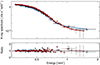 |
Fig. A.1. XMM-Newton X-ray spectra from the 2024 campaign EPIC-pn X-ray spectra, best-fitting models, and data-to-model ratio for the first (red) and fourth (blue) XMM-Newton observation of the 2024 campaign. |
A.2. Swift XRT
The Swift XRT observations were performed in Photon Counting (PC) mode and were analysed following the procedure outlined in Evans et al. (2007, 2009), which uses fully calibrated data and corrects for effects such as pile-up and the bad columns on the CCD, to obtain count rates on an observation-by-observation (or snapshot-by-snapshot) basis. Each observation typically comprises a couple of shorter exposure snapshots that have been also analysed following similar procedures to search for the occasional detection of one QPE (or part of it), although none was securely detected during the 2024 campaign. Specifically, the individual 0.3-1 keV count rates for every observation or snapshot exposure were obtained using the on-line XRT product generator tool8.
A.3. NICER
GSN 069 was observed by the Neutron Star Interior Composition ExploreR (NICER; Gendreau et al. 2016) for a total of 28 ks (PI: Miniutti, OBSIDs 7672010401-7672011101) from 17 May to 25 August 2024. We processed the data using HEASoft v6.33 and NICERDAS v11a. The quiescent flux of GSN 069 (∼4 − 6 × 10⁻¹³ erg cm−2 s−1) is comparable to the NICER observational background, which itself can vary significantly between snapshots. To reliably estimate the source flux over time, we followed the time-resolved spectroscopy procedure described in detail in Chakraborty et al. (2024), of which we give a brief summary here. We use nimaketime with unrestricted undershoot and overshoot event rates, and disabled event auto-screening on a per-focal plane module (FPM) basis; the typical resulting Good-Time Intervals (“GTIs”) lasted between 100-500 s, such that each OBSID was comprised of several GTIs spaced by 𝒪(few ks). In each GTI, we manually discard FPMs with 0-0.2 or 5-15 keV count rates > 3σ higher than the average, or above an absolute threshold of 20 counts sec−1; such events are likely due to extreme background contamination via the solar wind charge exchange or cosmic rays, rather than being related to intrinsic source variability. We then used the SCORPEON9 template-based background model, together with an additional source model represented by tbabs×zashift×diskbb, to jointly fit for the source- and background-contribution to each GTI in XSPEC. The resulting source fluxes were estimated using the cflux convolutional model component on the source model, and associated errors are 1-sigma. Fluxes over one observation (typically within a few hours) were then combined, and the mean and standard deviation is shown in Fig. 10 on an observation-by-observation basis.
Appendix B: Further O–C analysis in GSN 069
As discussed in Section 4.1, the QPE identification used to produce the O–C diagrams in Fig. 4 is not unique, and we report below results obtained with two different identifications for QPEs during the May 2019 observation that is the most uncertain as it is associated with the longest gap with respect to the previous one (∼107 d, the second longest being ∼29 d).
In the original version of the O–C analysis in Section 4.1, the first QPE in May 2019 was assumed to be the 211th even one. The two closest versions of O–C diagrams for GSN 069 are obtained by assuming that it is instead either the 211th or the 212th odd one (the identification of all other QPEs follows trivially). The net result is that all O–C data for the May 2019 observation shift upwards or downwards by half Ptrial with respect to the case shown in Fig. 4. The O–C diagrams for these two different QPE identifications are shown in Fig. B.1 and B.2 respectively.
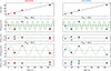 |
Fig. B.1. O–C diagrams for GSN 069: linear baseline model. Same as Fig. 4, but the first QPE in May 2019 is here identified with the 211th odd QPE. |
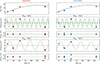 |
Fig. B.2. O–C diagrams for GSN 069: parabolic baseline model. Same as Fig. 4, but the first QPE in May 2019 is here identified with the 212th odd QPE. |
The O–C diagrams in Fig. B.1 are well described by a linear baseline model (solid line in the upper panels) plus a sinusoidal modulation, while no parabolic trend is needed so that Ṗorb = 0. On the other hand, the O–C diagrams for the alternative QPE identification shown in Fig. B.2 do require an additional parabolic trend (solid line in the upper panels) and are therefore associated with Ṗorb ≠ 0. As was the case for the O–C analysis in Section 4.1, a periodic modulation with either a ∼19 d or ∼43-44 d period is required in both cases. Results are reported in Table B.1 and Table B.2 for the Ṗorb = 0 and the Ṗorb ≠ 0 solutions respectively.
The orbital period Porb is always the same, within errors, for both odd and even QPEs regardless of Pmod and of the actual QPE identification, and it is also consistent with that obtained in Section 4.1. All other parameters (except Ṗorb, as obvious) are also consistent with the previous analysis at the few per cent level. The only significant difference between the three versions of the O–C diagrams we have produced is in the derived EMRI’s orbital evolution. We suggest three possible values associated with the three different identification of QPEs in May 2019, namely Ṗorb = 0, −3-4 × 10⁻⁵, or −6-7 × 10⁻⁵. As discussed in Section 4.2, the 2023 campaign on GSN 069 suggests that the intermediate value might be correct, although we consider the detection of Ṗorb ≃ −3.7 × 10⁻⁵ as tentative only due to the small number of independent measurements during the 2023 XMM-Newton campaign. The stability of best-fitting parameters despite the difference in QPE identification provides support to the robustness of the overall O–C analysis and derived parameters.
O–C analysis for GSN 069 leading to Ṗ = 0.
O–C analysis for GSN 069 leading to  .
.
As mentioned in Section 4.1, the number of data points in the odd QPEs (six) time series in Fig. 4 is the same that of the free parameters of the adopted model a + bx + cx2 + Amodsin(Pmod, ϕmod) prevented us to formally apply the model in that case. We then first considered fits to the even QPEs data (nine data points) and derived the best-fitting parameters and uncertainties. We then fitted the odd QPEs data by fixing one of model’s parameters to the best-fitting value derived from the even QPEs time series. The procedure was repeated by changing the value of the fixed parameter exploring a range of possible values much larger than the corresponding uncertainty from the even QPEs data best-fitting results. Specifically, we chose Porb because this is expected to be the same for both odd and even QPEs, and explored 17 ≤ Porb ≤ 19 h in steps of 0.01 h in the odd QPEs data. Choosing a different parameter did not produce any significant change in the results. With this procedure, we could estimate the allowed range for all parameters and compare them with results from the even QPEs time series. Results are reported in Table 1. The procedure turned out to be validated by the excellent agreement with the independent analysis of the even QPEs time series for all parameters, as well as with results discussed above, where independent fits on both odd and even QPEs data could be performed.
Appendix C: SMBH spin effects and numerical implementation
In this work, we made use of the numerical code presented in Franchini et al. (2023) who implemented a semi-analytic approach to numerically simulate the collisions between the accretion disc around a SMBH with mass M and the secondary orbiting companion with mass m ≪ M in an EMRI system. The accretion disc around the primary was assumed to extend down to the innermost stable circular orbit of a generic Kerr black hole, and to be prograde with respect to the SMBH spin that was assumed to be aligned with the z-axis (i.e. the disc’s angular momentum has also positive z-component). Based on the growing evidence for a connection between QPE systems and TDEs, the considered disc structure was assumed to be consistent with a TDE origin following earlier work by Franchini et al. (2016). The equations of motion of the EMRI were integrated up to the 3.5 post-Newtonian order, thus removing the test-particle approximation used in previous work (e.g. Xian et al. 2021), and including all relevant time delays (Roemer, Shapiro, and Einstein delays) from the impact position to the observer. For further details, we refer to the work by Franchini et al. (2023).
Rigid disc precession can be naturally implemented in the numerical code. Whenever the primary SMBH is spinning, and the disc misaligned, we assumed that the warp induced by the Lense-Thirring effect (Lense & Thirring 1918) propagates as a bending wave, allowing the disc to rigidly precess around the primary, spinning SMBH. In this regime, the disc precesses rigidly with a frequency that is the angular-momentum-weighted average of the Lense-Thirring precession frequency over the extent of the disc. In our work, however, to study the effects of disc precession alone without introducing unnecessary complications due to the EMRI orbit’s nodal precession induced by the spinning SMBH (see discussion below), we have included disc precession at an arbitrarily chosen period, keeping the SMBH black hole spin fixed to zero.
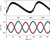 |
Fig. C.1. Primary SMBH spin effects: nodal precession. O–C diagrams for the same parameters as in Fig. 7, but where we have considered an almost maximally-rotating Kerr primary SMBH with dimensionless spin of χ = 0.9. The upper panel shows the O–C diagrams over slightly more than one nodal precession period (∼3 yr), while the lower panel are O–C diagrams derived from a restricted 160 d portion of the full light curve, commensurate with the baseline that is probed in GSN 069 by observations between December 2018 and May 2019 (see Fig. 3 and 4). |
Whenever the SMBH is spinning, and even in absence of disc precession, the EMRI orbit is affected because, in addition to the in-plane apsidal precession that is present also for a non-spinning SMBH, it is subject to nodal precession of the orbital plane at the nodal precession frequency. Nodal precession affects the QPEs timing properties in a similar way as disc precession, introducing a coherent modulation of QPEs arrival times that induces correlated O–C diagrams for odd and even QPEs at the nodal precession timescale. However, the nodal precession timescale is generally much longer than the disc precession and apsidal precession ones, so that its effects are likely to be important only on very long timescales, typically much longer than the baseline spanned by QPEs observations. The effect of nodal precession on the O–C diagrams is shown in Fig. C.1 where we assumed exactly the same parameters as those resulting in Fig. 7, but considered the case of an almost maximally-spinning Kerr SMBH with dimensionless spin χ = 0.9. In the upper panel of Fig. C.1, we show the O–C diagrams on a relatively long baseline covering slightly more than one nodal precession timescale. The precession of the EMRI orbital plane introduces a long-term correlation between the O–C diagrams of odd and even QPEs on the nodal precession timescale. However, on a baseline only comprising a few apsidal precession timescales, the O–C diagrams for the two branches are still nearly perfectly anti-correlated as shown in the lower panel, where we selected randomly a 160 d time interval from the simulation to mimic the baseline of GSN 069 observations (see Fig. 3 and, e.g., 4), and repeated the O–C analysis.
As mentioned, the nodal precession timescale is always significantly longer than the apsidal one (∼3 yr versus ∼50 d for the case shown in Fig C.1), so that black hole spin effects can only be revealed by very long-term, high-cadence monitoring campaigns. As we are here typically interested with observations spanning at most a few apsidal precession timescales, we do not discuss nodal precession of the EMRI orbital plane. However, its effects may be needed to interpret the long term-behaviour of at least some QPE sources in the future.
The simulations involving a hierarchical triplet have been performed leveraging on the computational framework developed in Bonetti et al. (2016, 2018). Specifically, the code integrates the equations of motion of three-body systems exploiting the high accuracy Bulirsch-Stoer integration scheme. The numerically obtained trajectories were computed from Post-Newtonian three-body Hamiltonian featuring correction up to 2.5 PN order. The framework, by allowing generic mass ranges for the three bodies, can be initialised to evolve an EMRI system perturbed by a third object. In more details, the system was initialised with an inner binary M1 − m and and outer binary effectively formed by M1 + m and M2. Here, m < < M1 ∼ M2. For the specific simulations of this work, the three-body code has been complemented with a routine to detect the crossing of a disc orbiting around M1. Each time the trajectory of m intercepted the plane defined by the accretion disc, its coordinates and the crossing time were recorded. The procedure closely follows the one employed in Franchini et al. (2023). Once the time of crossing was recorded, it was complemented by the appropriate time-delays (Roemer, Shapiro and Einstein) referred to a distant observer, as done in Franchini et al. (2023). Specifically, we expressed the arrival time to the distant observer as (see e.g. Poisson & Will 2014, sec. 10.3.6) as:
 (C.1)
(C.1)
where the three delays are given by the following expression:
 (C.2)
(C.2)
 (C.3)
(C.3)
 (C.4)
(C.4)
Here, M = M1 + M2 is the mass of the binary, while robs denotes the observer position. r1 and r2 represent instead the position vectors of the primary and secondary SMBH with respect to the centre of mass of the system, while the unit vector k is given by:
 (C.5)
(C.5)
Finally, a, e, and u respectively represent the orbit semi-major axis, eccentricity and eccentric anomaly, respectively. The time series of (observed) crossing times, associated with QPEs, were then used to compute the O–C plots and all other relevant quantities.
Appendix D: Schematic representation of the proposed modulations
In Fig. D.1, we show a schematic representation of the effect of apsidal precession and of the proposed external modulations on O–C diagrams. At each impact, two-sided, hot and expanding plasma clouds are ejected from the disc, and are responsible for QPEs (Franchini et al. 2023; Linial & Metzger 2023). The clouds colour-code distinguishes between impacts at the ascending and descending nodes that are associated with, e.g., odd and even QPEs. Each panel comprises three different sub-panels. The first two represent two different time snapshots of the system geometry and the resulting QPE light curve where the dashed blue and red lines indicate the QPE arrival times expected if QPEs of the same parity recur on a constant period, as is the case for a Keplerian EMRI orbit. The leftmost sub-panel shows the resulting O–C diagrams.
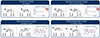 |
Fig. D.1. Schematics of the effect of apsidal precession and external modulations on O–C diagrams. The upper panels show the case of a Keplerian EMRI orbit (left) and of a General Relativistic one including apsidal precession (right). The lower two panels are associated with the two modulating scenarios we considered in our work: disc precession (left) and a hierarchical triple model in which an outer SMBH forms a tight SMBH binary with the inner EMRI system (right), see text for details. |
In the upper-left panel of Fig. D.1, we show the case of a Keplerian EMRI orbit. As the Keplerian orbit is fixed, impacts occur always at the same site on the disc, and consecutive odd (even) QPEs are always separated by the same time interval, corresponding to the EMRI orbital period. The O–C data for odd and even QPEs align on a straight line and, once a linear ephemeris is removed, they are actually all zero. The upper-right panel shows the effects of General Relativistic apsidal precession of the EMRI orbit. Impacts at the ascending nodes (odd QPEs) are delayed with respect to the Keplerian expectation, while the corresponding ones at the descending nodes (even QPEs) are anticipated by a similar time interval (or vice-versa). Therefore, the O–C diagrams for odd and even QPEs are modulated on the apsidal precession timescale and are in phase opposition. The amplitude of the modulation is of the order of few minutes for typical EMRI parameters and observer inclination.
The lower panels of Fig. D.1 show the effects of the two external modulation scenarios considered in our work, namely rigid disc precession (lower-left) or the presence of an outer SMBH forming a SMBH binary with the inner EMRI system (lower-right). In both cases, if the ascending impact is delayed (anticipated) with respect to the Keplerian expectation, the corresponding impacts at the descending node is also delayed (anticipated). The O–C diagrams for odd and even QPEs are therefore modulated on the external timescale (disc precession or outer SMBH binary orbital period) with minimal phase difference. A small phase difference is expected due to the fact that impacts at the ascending and descending nodes are not simultaneous but separated by the average recurrence time between an ascending node impact and the subsequent descending node one (< Trec > ≃9 h in GSN 069).
All Tables
All Figures
|
Fig. 1. Schematic representation of a QPE time series comprising four consecutive QPEs. Odd and even QPEs represent impacts through the ascending and descending nodes respectively (or vice versa). The definition of the different QPE recurrence times that are used to compute Papp and eapp is highlighted (see Eqs. (1)–(3) and text for details). |
| In the text | |
|
Fig. 2. Effects of apsidal precession on secondary-disc impacts. We show two different apsidal phases leading to |
| In the text | |
|
Fig. 3. QPE timing properties in GSN 069. In the upper row, we show the X-ray 0.4–1 keV light curves of GSN 069 used in this work. The first two and last light curves are from the EPIC-pn camera on board XMM-Newton, while the third is from the ACIS-S detector on board Chandra. The latter light curve has been re-scaled to the expected EPIC-pn count rate (as in Miniutti et al. 2023a). XMM-Newton data could be used down to 0.2 keV but, since QPE properties (peak time and overall duration) are energy-dependent (Miniutti et al. 2019), we use here a common energy band down to 0.4 keV only in order to make use also of the Chandra data. The three lower rows show Trec, Papp, and eapp as obtained from the QPE peak times. Due to the gaps in the data the colour code distinguishing odd from even QPEs during different observations might be different from the one shown here where we arbitrarily assigned all stronger (weaker) QPEs to the even (odd) time series. |
| In the text | |
|
Fig. 4. O–C diagrams for GSN 069. We show the O–C diagrams for odd (left) and even (right) QPEs for GSN 069 resulting from identifying the first QPE of the May 2019 observation with the 211th even QPE. The upper panels show the O–C data together with the linear plus parabolic baseline model for Pmod ≃ 19 d. The lower panels show the corresponding residuals (O–CBASELINE) as well as the ones corresponding to the full best-fitting model including a sinusoidal modulation (O–CFULL) for the two possible Pmod. The sinusoidal modulation is also shown in the O–CBASELINE to guide the eye. |
| In the text | |
|
Fig. 5. Pmod detection in the O–C diagrams. We show Δχ2 as a function of modulating period Pmod for the final best-fitting model to the O–C diagrams in Fig. 4. Odd QPEs are shown in red, even ones in blue. We explored a wide range of Pmod between 4 d and 90 d, and all other local minima are noisy (i.e. neighbouring data points to the local minimum have much higher Δχ2 value). |
| In the text | |
|
Fig. 6. 2023 campaign on GSN 069. In the upper panel, we show the XMM-Newton EPIC-pn light curve from the May 2019 observation, together with a representative best-fitting model. The EPIC-pn light curves from the 2023 campaign are shown in the lower panels. We aligned the last QPEs of these latter observations with one of the QPEs in the upper panel to ease comparison, and we also reproduced the best-fitting model for the May 2019 light curve in the lower panels. |
| In the text | |
|
Fig. 7. QPE timing from the impact model. We show Trec, Papp, eapp, and the O–C diagrams for a nearly circular EMRI orbit with eccentricity e = 0.05, and parameters commensurate with those of GSN 069. Odd and even QPEs are shown in red and blue respectively. We point out that the data points in the lower panels (O–C diagrams) are not exactly aligned with those in the upper ones. This is because the abscissa of a given data point in O–C diagrams is a multiple of Ptrial rather than the observed QPE arrival time. |
| In the text | |
|
Fig. 8. Disc precession solution for GSN 069. In the upper three panels, we show Trec, Papp, and the O–C diagrams for a disc precession solution with Pdisc ∼ 44 d for GSN 069 (see text for further details). The lower panel shows the O–C diagrams for the same simulation but with Pdisc ∼ 19 d. |
| In the text | |
|
Fig. 9. Hierarchical triple solution for GSN 069. In the upper three panels we show Trec, Papp, and the O–C diagrams for a hierarchical triple solution for GSN 069 comprising the inner, QPE-emitting EMRI and an outer circular SMBH binary with orbital period Pout = 44 d. The O–C diagrams for the alternative solution with Pout = 19 d are shown in the lower panel. |
| In the text | |
|
Fig. 10. 2024 Swift and NICER monitoring campaign. We show the normalised 0.3–1 keV quiescent light curves of GSN 069 as obtained by the Swift XRT and by NICER during the current campaign. Any two consecutive Swift observations with consistent count rates have been combined to reduce the statistical uncertainty. Individual NICER snapshots have been analysed separately, and the data points represent the mean 0.3–1 keV flux and standard deviation obtained within a few hours. The dashed line is a sine function modulation with period ≃19.9 d and semi-amplitude ≃45% resulting in χ2 = 31 for 17 degrees of freedom. |
| In the text | |
|
Fig. 11. Folded Swift and NICER light curve. The upper panel shows the light curve of Fig. 10 folded at the best-fitting period of 19.9 d. Two cycles are shown for visual clarity, and the distinction between Swift and NICER data points has been removed. The solid red line represents the sinusoidal modulation with 1σ uncertainties in its amplitude shown as dotted lines. In the lower panel, we show the predicted modulation from Doppler boosting (blue) as well as one possible realisation of the disc precession model (red) corresponding to a disc misalignment of idisc = 20° and observer inclination iobs = 45°. |
| In the text | |
|
Fig. 12. Zoom of Fig. 10 over a restricted MJD range in which eight XMM-Newton observations are also available (green crosses). The XMM-Newton data points show the 0.3–1 keV average X-ray flux during each XMM-Newton observation, normalised to the best-fitting constant model over the spanned baseline. Uncertainties on the XMM-Newton data are included, but smaller than symbol size. |
| In the text | |
|
Fig. A.1. XMM-Newton X-ray spectra from the 2024 campaign EPIC-pn X-ray spectra, best-fitting models, and data-to-model ratio for the first (red) and fourth (blue) XMM-Newton observation of the 2024 campaign. |
| In the text | |
|
Fig. B.1. O–C diagrams for GSN 069: linear baseline model. Same as Fig. 4, but the first QPE in May 2019 is here identified with the 211th odd QPE. |
| In the text | |
|
Fig. B.2. O–C diagrams for GSN 069: parabolic baseline model. Same as Fig. 4, but the first QPE in May 2019 is here identified with the 212th odd QPE. |
| In the text | |
|
Fig. C.1. Primary SMBH spin effects: nodal precession. O–C diagrams for the same parameters as in Fig. 7, but where we have considered an almost maximally-rotating Kerr primary SMBH with dimensionless spin of χ = 0.9. The upper panel shows the O–C diagrams over slightly more than one nodal precession period (∼3 yr), while the lower panel are O–C diagrams derived from a restricted 160 d portion of the full light curve, commensurate with the baseline that is probed in GSN 069 by observations between December 2018 and May 2019 (see Fig. 3 and 4). |
| In the text | |
|
Fig. D.1. Schematics of the effect of apsidal precession and external modulations on O–C diagrams. The upper panels show the case of a Keplerian EMRI orbit (left) and of a General Relativistic one including apsidal precession (right). The lower two panels are associated with the two modulating scenarios we considered in our work: disc precession (left) and a hierarchical triple model in which an outer SMBH forms a tight SMBH binary with the inner EMRI system (right), see text for details. |
| In the text | |
Current usage metrics show cumulative count of Article Views (full-text article views including HTML views, PDF and ePub downloads, according to the available data) and Abstracts Views on Vision4Press platform.
Data correspond to usage on the plateform after 2015. The current usage metrics is available 48-96 hours after online publication and is updated daily on week days.
Initial download of the metrics may take a while.