| Issue |
A&A
Volume 674, June 2023
|
|
|---|---|---|
| Article Number | L1 | |
| Number of page(s) | 10 | |
| Section | Letters to the Editor | |
| DOI | https://doi.org/10.1051/0004-6361/202346653 | |
| Published online | 31 May 2023 | |
Letter to the Editor
Alive and kicking: A new QPE phase in GSN 069 revealing a quiescent luminosity threshold for QPEs
1
Centro de Astrobiología (CAB), CSIC-INTA, Camino Bajo del Castillo s/n, ESAC campus, 28692 Villanueva de la Cañada, Madrid, Spain
e-mail: This email address is being protected from spambots. You need JavaScript enabled to view it.
2
MIT Kavli Institute for Astrophysics and Space Research, Massachusetts Institute of Technology, Cambridge, MA 02139, USA
3
Telespazio-Vega UK for ESA, Operations Department, European Space Astronomy Centre (ESAC), Villanueva de la Cañada, 28692 Madrid, Spain
4
Department of Physics & Astronomy, University of Leicester, Leicester LE1 7RH, UK
Received:
14
April
2023
Accepted:
10
May
2023
Abstract
X-ray quasi-periodic eruptions (QPEs) are intense repeating soft X-ray bursts from the nuclei of nearby galaxies. Their physical origin is still largely unconstrained, and several theoretical models have been proposed ranging from disc instabilities to impacts between an orbiting companion and the existing accretion disc around the primary, or episodic mass transfer at pericentre in an extreme mass-ratio binary. We present here results from a recent XMM-Newton observation of GSN 069, the galactic nucleus where QPEs were first discovered. After about two years of absence, QPEs have reappeared in GSN 069, and we detect two consecutive QPEs separated by a much shorter recurrence time than ever before. Moreover, their intensites and peak temperatures are remarkably different, a novel addition to the QPE phenomenology. We study the QPE spectral properties from all XMM-Newton observations assuming QPEs to either represent an additional emission component superimposed on that from the disc, or the transient evolution of the disc emission itself. In the former scenario, QPEs are consistent with black-body emission from a region that expands by a factor of 2–3 during the individual QPE evolution with radius ≃5 − 10 × 1010 cm at QPE peak. In the alternative non-additive scenario, QPEs originate from a region with an area ∼6 − 30 times smaller than the quiescent state X-ray emission, with the smallest regions corresponding to the hottest and most luminous eruptions. The QPE reappearance reveals that eruptions are only present below a quiescent luminosity threshold corresponding to an Eddington ratio λthresh ≃ 0.4 ± 0.2 for a 106 M⊙ black hole. The disappearance of QPEs above λthresh is most likely driven by the ratio of QPE to quiescence temperatures, kTQPE/kTquiesc, approaching unity at high quiescent luminosity, making QPE detection challenging, if not impossible, above threshold. We briefly discuss some of the consequences of our results on the proposed models for the QPE physical origin.
Key words: galaxies: nuclei / galaxies: individual: GSN 069 / accretion, accretion disks / black hole physics / X-rays: individuals: GSN 069
Einstein Fellow.
© The Authors 2023
 Open Access article, published by EDP Sciences, under the terms of the Creative Commons Attribution License (https://creativecommons.org/licenses/by/4.0), which permits unrestricted use, distribution, and reproduction in any medium, provided the original work is properly cited.
This article is published in open access under the Subscribe to Open model. This email address is being protected from spambots. You need JavaScript enabled to view it. to support open access publication.
1. Introduction
First discovered in the nucleus of the galaxy GSN 069 (Miniutti et al. 2019), X-ray quasi-periodic eruptions (QPEs) are one of the most recent examples of extreme X-ray variability associated with supermassive black holes (SMBHs). QPEs are fast intense soft X-ray bursts repeating every few hours that stand out with respect to an otherwise stable quiescent X-ray emission, likely from an existing accretion disc. Following their first detection in GSN 069, QPEs have been identified in the nuclei of other four galaxies to date: RX J1301.9+2747 (Giustini et al. 2020), eRO-QPE1 and eRO-QPE2 (Arcodia et al. 2021, 2022), and XMMSL1 J024916.6-04124 (Chakraborty et al. 2021). A further QPE candidate is 2XMM J123103.2+110648 (Terashima et al. 2012), although its X-ray variability is more reminiscent of a quasi-periodic oscillation (QPO) than of QPEs (Lin et al. 2013; Webbe & Young 2023), and the source has been proposed to represent a descendant of QPE sources (King 2023b).
Quasi-periodic eruptions have thermal-like X-ray spectra with temperatures evolving from kT ≃ 50 − 80 eV to ≃100 − 250 eV and back in about one to few hours with duty cycle (duration over recurrence) of 10–30% and peak X-ray luminosity of 1042–1043 erg s−1, depending on the specific source. QPE host galaxies harbour SMBHs of relatively low mass (≃105 − 107 M⊙ at most), and they are best classified as post-starburst galaxies (Wevers et al. 2022), a population that is similar to the preferred tidal disruption events (TDEs) hosts, as is the low SMBH mass (Arcavi et al. 2014; French et al. 2020). Two out of the five currently known QPE sources, GSN 069 and XMMSL1 J024916.6-04124, have been directly associated with X-ray TDEs (Shu et al. 2018; Sheng et al. 2021; Miniutti et al. 2023; Chakraborty et al. 2021). A further QPE candidate was found during the X-ray decay of an optically detected TDE, strengthening the possible connection between QPEs and TDEs (Quintin et al. 2023). Despite being unobscured in the X-rays, optical and UV spectra never show signs of broad emission lines (BELs; see Wevers et al. 2022). The lack of BELs indicates either that an active nucleus switched off leaving only relic narrow lines, or that the accretion flow is unable to support a mature broad line region, perhaps being too compact, as expected for instance in TDEs.
We focus here on the discovery-source, GSN 069 (see also Miniutti et al. 2013), whose long-term evolution over the past ∼12 yr has been discussed by Miniutti et al. (2023) together with the main properties of its QPEs. The evolution has so far been consistent with two repeating, possibly partial X-ray TDEs about 9 yr apart (hereafter TDE 1 and TDE 2), although it is difficult to exclude a different origin for the observed long-term X-ray variability as the luminosity has decayed by only a factor of a few in ∼9 yr. A set of 15 QPEs with well-defined properties were detected in four observations performed towards the end of the decay of TDE 1 (XMM3 to XMM5 in Table D.1, where all high-quality observations of GSN 069 are reported). These QPEs (hereafter referred to as regular QPEs) were separated by ≃32 ks on average. QPE intensities alternated, and stronger (weaker) QPEs were systematically followed by longer (shorter) recurrence times with Tlong ≃ 33 ks (Tshort ≃ 31 ks) on average. Moreover, the higher (lower) the intensity ratio between consecutive QPEs, the longer (shorter) the recurrence time between them. A further set of four weaker QPEs was detected in an XMM-Newton observation performed during the rise of TDE 2 (XMM6 in Table D.1), when the quiescent level was significantly brighter than in any previous observation with QPEs. This set of weaker QPEs (hereafter referred to as irregular QPEs) broke the previous regular patterns and, while intensities still roughly alternated, recurrence times did not, signalling that the system was undergoing major change at that epoch (possibly consistent with XMM6 being performed during the rise of TDE 2). During all XMM-Newton observations with regular QPEs, a lower intensity QPO of the otherwise stable quiescent emission was also detected with period equal to the average recurrence time between consecutive QPEs. Such QPO-like variability was absent during the XMM6 observation with weaker irregular QPEs. Eruptions have since then disappeared, as demonstrated by long-enough exposures from May 2020 to December 2021 (XMM7 to XMM11 in Table D.1).
We report results from a new XMM-Newton observation of GSN 069 performed on 7 July 2022, about seven months after the last observation where no QPEs were detected. As the overall X-ray flux was decaying after TDE 2, searching for the reappearance of QPEs at flux levels similar to the previous regular QPE phase was the main motivation for observing GSN 069 with XMM-Newton. We used the same data reduction procedures of Miniutti et al. (2023) for all X-ray observations and we refer to their work for details.
2. A new QPE phase
The EPIC pn, MOS1, and MOS2 0.2 − 1 keV light curves during the new XMM-Newton observation (hereafter XMM12) are shown in Fig. 1 and demonstrate that relatively high-amplitude QPEs have reappeared in GSN 069 after 2.0 ± 0.5 yr of absence. As done in previous QPE analyses (Miniutti et al. 2023), we fitted the EPIC pn light curves with a baseline phenomenological model comprising a constant, representing the quiescent level emission, and two Gaussian functions describing the QPEs. The fit was performed in both the 0.2–1 keV and the 0.4–1 keV bands to ease comparison with previous work where the restricted energy band was used to include three QPEs from a Chandra observation. Results are reported in Table D.2.
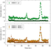 |
Fig. 1. EPIC light curves from the XMM12 observation. Light curves in the 0.2 − 1 keV with time bins of 200 s (pn) and 400 s (MOS) are shown. Background light curves, rescaled to the same extraction area, are also shown to highlight the slightly higher background during the initial ∼10 ks of the EPIC exposures. The start of the MOS 1 exposure is taken as origin for the time-axis in all cases. |
We detect one weak and one strong QPE during XMM12, separated by ≃20 ks. The separation is significantly shorter than the typical recurrence time during the previous regular QPE phase (≃32 ks), and even than the shortest recurrence time ever detected during the irregular XMM6 observation (≃26 ks). No QPEs are detected in the first ≃27 ks of the EPIC exposures. QPEs are therefore no longer strictly quasi-periodic or, at least, the difference between long and short recurrence times has significantly increased with respect to the previous QPE phase. The intensity ratio between the weak and strong QPE in XMM12 (≃0.26 in the 0.2–1 keV band) is also much lower than between any consecutive QPE pair in the previous regular phase (≳0.67).
As is clear in Fig. 1, the quiescent level during the XMM12 observation is not constant during the exposure, but exhibits variability on timescales of a few tens of ks. In order to study it in more detail, we rebinned the original light curve by a factor of five to increase the signal-to-noise ratio. In the upper panel of Fig. 2, we show the rebinned EPIC pn light curve together with the best-fitting baseline model resulting in χ2 = 550 for 49 degrees of freedom. While the model describes QPEs well, the overall statistical quality of the fit is very poor. Residuals for the baseline model fit are shown in the middle panel of Fig. 2. The shape of the residuals suggest a possible sinusoidal modulation, or QPO, as indicated by the solid line (plotted to guide the eye). By refitting the original light curve (upper panel) with the addition of a sine function, the statistical quality of the fit improves by Δχ2 = −410 for three degrees of freedom, and the resulting residual light curve is shown in the lower panel of Fig. 2. We derive a best-fitting period P = 54 ± 4 ks, and the results are reported in Table D.3.
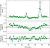 |
Fig. 2. Quiescent level QPO. Upper panel: 0.2–1 keV pn light curve with time bins of 1000 s, together with its baseline best-fitting model. Middle panel: Resulting residuals and, as a solid line, a sine function that is plotted to guide the eye. Lower panel: Residuals once the original light curve is fitted by adding a sine function to the baseline model. |
As only one cycle is detected and, furthermore, with a period suspiciously similar to the exposure duration, the observed QPO candidate cannot be considered significant from a statistical point of view. Moreover, the QPO period P ≃ 54 ks is different from that detected in the previous regular QPE phase (≃32 ks), so that previous QPOs do not enhance, at least formally, the QPO significance in XMM12. On the other hand, the very fact that a QPO was consistently detected in all XMM-Newton exposures during the previous regular QPE phase (Miniutti et al. 2023) suggests the need to explore the QPO candidate in XMM12 further.
3. Properties of the new QPE phase
The data so far suggest that QPEs and QPOs are linked and could represent different aspects of the same phenomenon (see Miniutti et al. 2023, Sect. 4). We cannot exclude that QPOs represent secondary, longer-lived (broader) QPEs with duty cycles ∼100% that follow the primary ones with a delay of 8–10 ks. Moreover, the QPO (or secondary QPE) is only present following strong enough QPEs (see Appendix A). During the XMM12 observation, the weak QPE has roughly the same intensity as the irregular ones in XMM6 that were not associated with a QPO (see e.g. Fig. 5 or C.1). We then speculate that the period of the QPO candidate in XMM12 is representative of the typical separation between strong QPEs only,  , rather than between consecutive QPEs, so that
  ks in the new QPE phase.
There is another independent way to estimate the recurrence time  between QPEs of the same type during XMM12. As discussed in Appendix A, the correlation between the intensity ratio of consecutive QPEs and the recurrence time between them can be used to infer
  ks. This is fully consistent with the estimate obtained from the QPO-like variability and the two independent estimates overlap for
  ks. Then, by definition, one has
  ks and
  ks (and, possibly, ≃33 ks) in the new QPE phase, to be compared with
  ks and
  ks summing up to
  ks in the old (regular) QPE phase. The recurrence time fluctuation ΔTrel = (Tlong−Tshort)/⟨Trec⟩ (where ⟨Trec⟩=Tsum/2), then increased from ≃6% in the old phase to ≳30% in the new one. Figure 3 shows a comparison between old and new QPE phases together with a possible extrapolation of the new phase to longer timescales based on the (somewhat speculative) arguments presented above.
 |
Fig. 3. Comparison between old and new QPE phases. Upper panel: Typical model light curve for observations during the old regular QPE phase. Lower panel: Qualitative representation of the light curve from the XMM12 observation (new QPE phase; solid line) and one possible extrapolation of longer-term behaviour based on the arguments discussed in Sect. 3 and Appendix A (dashed line). The light curves were normalised so that the intensity of the strong QPEs is the same in both panels. The same quiescent level is assumed for visual clarity. |
4. Quiescent luminosity threshold for QPEs
To place all QPE observations in context, we updated the quiescent Lbol long-term light curve of GSN 069 in Fig. 4 (see Table D.1). This is the same as Fig. 20 in Miniutti et al. (2023), with the addition of the XMM12 observation and of one data point from the latest Neil GehrelsSwift monitoring (actually comprising a few short exposures combined). Figure 4 shows that QPEs are not found in the highest luminosity observations, and are instead observed only below a quiescent bolometric luminosity threshold Lthresh ≃ 3 × 1043 erg s−1. Assuming, for ease of scaling, a black hole mass of MBH = 106 M⊙, and considering the systematic uncertainties on the estimated bolometric luminosity discussed in Miniutti et al. (2023), the luminosity threshold translates into an Eddington ratio threshold of λthresh ≃ 0.4 ± 0.2. We note that we define λthresh as that below which QPEs are present. On the other hand, QPEs are absent above a slightly higher threshold (a factor of ≃1.3) because of the luminosity gap with no observations (see Fig. 4).
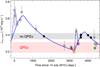 |
Fig. 4. Quiescent luminosity long-term evolution. Shown is the Lbol evolution of the quiescent emission over the past ∼12 yr. The dotted-solid line is a possible model discussed in Miniutti et al. (2023). The grey data points refer to observations that are too short to ensure the detection of QPEs (squares for Swift and circles for XMM-Newton data). Coloured and black data points represent instead long enough observations respectively with and without QPEs. The purple star denotes the XMM6 observation with irregular QPEs. A Chandra observation (exhibiting three QPEs) performed between the XMM4 and XMM5 observations was omitted as the corresponding quiescent luminosity is highly uncertain (see Table D.1). |
In order to study the QPE spectral properties, we first assumed that QPEs are an additional component with respect to disc emission, and we extracted intrinsic quiescence-subtracted X-ray spectra of all QPE peaks, modelling them with a simple absorbed black body (see Appendix B). Figure 5 shows the bolometric QPE luminosity (at peak) as a function of rest-frame temperature. The regular QPEs (XMM3 to XMM5) peak at 3.7–5.2 × 1042 erg s−1 with a typical temperature of 90–100 eV (with a colder outlier during XMM5). The irregular QPEs (XMM6) are significantly less luminous (and colder) than the regular ones. The strong and weak QPEs in the new phase (XMM12) are remarkably consistent with the previously detected regular and irregular QPEs respectively.
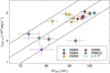 |
Fig. 5. QPE Lbol–T relation. The QPE-only Lbol is shown as a function of QPE rest-frame temperature from quiescence-subtracted QPE spectra assuming a simple absorbed black-body model. The dotted lines show Lbol ∝ T4 relations with different normalisation. The actual best-fitting relation is somewhat shallower with index ≃3.1. |
The data are best described by an Lbol ∝ Tq relation with q = 3.1 ± 0.2. However, as is clear from Fig. 5, a q = 4 solution (dotted lines) corresponding to constant-area black-body emission cannot be excluded with high significance. Assuming black-body emission and an emitting area A = 4πR2, QPEs at peak are consistent with an emitting region with Rpeak ≃ 5 − 10 × 1010 cm, where we ignore potentially relevant scattering effects (Mummery 2021). We also point out that, since QPEs only carry ∼10 − 20% of the overall bolometric luminosity (Miniutti et al. 2019, 2023), they become undetectable once their intrinsic temperature is of the order of that of the quiescent emission. The lack of QPEs above λthresh can therefore be taken as an indication that the contrast between QPE peak and quiescent temperatures is intrinsically close to unity above threshold, making it impossible to unambiguously identify QPEs against the quiescent emission. As discussed in Appendix C, the lack of QPEs above threshold is most likely intrinsic, and not just an effect of the brighter (and hotter) quiescent level. On the other hand, if QPEs are not an extra component superimposed on the disc emission, they must originate from an area ∼6–30 times smaller than that associated with the quiescent state, the smallest regions being associated with the hottest, most luminous QPEs (see Appendix B).
5. Discussion
Several theoretical models have been presented to explain the physical origin of the QPE phenomenon. They are based on different flavours of disc instabilities (Raj & Nixon 2021; Pan et al. 2022, 2023; Kaur et al. 2022; Śniegowska et al. 2023), impacts between an orbiting companion in an extreme mass-ratio inspiral (EMRI) system and the existing accretion flow about the primary (Suková et al. 2021; Xian et al. 2021; Linial & Metzger 2023; Franchini et al. 2023; Tagawa & Haiman 2023), or episodic mass transfer at pericentre from stars or white dwarfs in a variety of configurations (King 2020, 2022, 2023a; Chen et al. 2022; Wang et al. 2022; Zhao et al. 2022; Metzger et al. 2022; Lu & Quataert 2022; Krolik & Linial 2022; Linial & Sari 2023). Our observational results present new challenges for all theoretical models proposed to date, and we briefly discuss some of their implications below.
Recurrence time variation. Models invoking mass transfer at pericentre as well as the majority of disc instability models predict strictly periodic behaviour for consecutive QPEs with Tlong ≃ Tshort. Some fluctuation of the recurrence time is expected, but the observed ΔTrel ≳ 30% in the new phase (and its factor of ≳5 increase with respect to the previous phase) is likely too large to be accounted for naturally (King 2022; Krolik & Linial 2022; Linial & Sari 2023). In the case of disc-secondary impacts, where two QPEs per orbit are produced, the difference between Tlong and Tshort in the previous regular phase could be explained by assuming a nearly circular orbit with eccentricity e ≃ 0.05–0.1. Hence, within the impacts model, the ΔTrel variation could be related to an increase of the EMRI orbital eccentricity between the old and new QPE phases (from e ≃ 0.05–0.1. to e ≳ 0.3). This could be achieved, for instance, by interaction with a third body through the Zeipel-Lidov-Kozai mechanism (see the review by Naoz 2016). In GSN 069, the third body might actually be an evolved star on a ≃9 yr period orbit that was partially disrupted twice at pericentre giving rise to TDE 1 and TDE 2 (Miniutti et al. 2023). If the secondary EMRI component is a star, eccentricity (and period) variation may also arise due to extreme mass-transfer episodes (perhaps inducing TDE 2) between the two QPE phases (Manukian et al. 2013; Gafton et al. 2015), as discussed by Linial & Metzger (2023).
Quiescence Eddington ratio threshold for QPE appearance. Models in which QPEs represent the fast transient evolution of the disc emission naturally depend on disc properties and might therefore be made consistent with the quiescent luminosity threshold. These include disc instability models (see e.g. Raj & Nixon 2021; Śniegowska et al. 2023; Pan et al. 2023), burst of mass accretion rate limited to the very innermost regions (possibly consistent with mass transfer from a highly eccentric orbit; see King 2020, 2022; Chen et al. 2022; Wang et al. 2022), or the transient formation of an inner, optically thick warm corona (Miniutti et al. 2019). Considering disc instabilities as representative examples, the disc may stabilise at high mass accretion rates or the instability period may increase to the extent that QPEs are undetected during typical XMM-Newton exposures (see Pan et al. 2023).
On the other hand, models in which QPEs are an extra emission component superimposed on that from the disc appear to be viable only if QPEs are produced by an interaction with the existing flow as independent additive QPEs with typical properties (luminosity and temperature) would have been easily detected even above threshold (see Appendix C). Additive QPE models in which QPEs originate from an interaction with the accretion flow include, for instance, disc-secondary impacts (Xian et al. 2021; Linial & Metzger 2023; Franchini et al. 2023; Tagawa & Haiman 2023), and shocks between the incoming streams and the disc in mass transfer scenarios (Lu & Quataert 2022). We have also shown that the lack of QPEs at high luminosities is most likely associated with a QPE-to-quiescence temperature ratio kTQPE/kTquiesc ∼ 1 above λthresh. This appears to be qualitatively consistent with the work of Lu & Quataert (2022) and Franchini et al. (2023), who show that the temperature ratio decreases with increasing accretion rate, asymptotically reaching unity in the latter model. As a final remark, we note that the luminosity threshold could be artificial, and QPEs might instead only appear with a certain delay with respect to the TDE peaks (see Fig. 4).
6. Conclusions
A new XMM-Newton observation in July 2022 shows that QPEs have reappeared in GSN 069 after ∼2 yr of absence. We detect one weak and one strong QPE separated by ≃20 ks, a significantly shorter recurrence time than ever observed before. The lack of QPEs during the first ≃27 ks of the XMM-Newton exposures implies that QPEs are no longer strictly quasi-periodic or that, at least, Trec fluctuations are now ΔTrel ≳ 30%, a factor of ≳5 larger than in the previous phase. Under the strong assumption that the new QPE phase behaves similarly to the previous regular one, we suggest that the recurrence time between consecutive QPEs of the same strong or weak type has decreased from  ks to
ks to  ks, a speculation that can be tested with future long X-ray observations. The intensity and temperature of the two consecutive QPEs in the new phase are remarkably different, unlike at any epoch observed previously.
Assuming QPE to represent an extra component superimposed on disc emission, the analysis of all quiescence-subtracted QPE spectra, together with previous results (Miniutti et al. 2023), shows that QPEs are consistent with a region that expands by a factor of 2–3 during the individual QPE evolution, reaching a radius Rpeak ≃ 5–10 × 1010 cm at peak (ignoring scattering). Further expansion decreases the contrast between QPE and quiescence temperatures and leads to the individual QPE decay. If QPEs are instead associated with the fast evolution of the accretion flow itself, they must originate from a region with area ∼6 − 30 times smaller than that associated with the quiescent state, the hottest (and most luminous) QPEs being associated with the smallest emitting regions.
We also show that QPEs only appear below an Eddington ratio threshold λthresh ≃ 0.4 ± 0.2 of the quiescent emission, where we assumed a 106 M⊙ for ease of scaling. If the threshold is confirmed by future observations, QPE models where the disc plays an important role appear to be particularly appealing. Models should account for the QPE disappearance above threshold and we show that this is likely induced by a QPE-to-quiescence temperature ratio kTQPE/kTquiesc ≃ 1 above λthresh. Theoretical models for the origin of QPEs face the challenge of explaining self-consistently the large variation in ΔTrel from the old to the new phase and the associated short recurrence time between consecutive QPEs in XMM12, as well as the presence of two consecutive QPEs with very different intensities and temperatures at the same epoch. Future long uninterrupted observations with XMM-Newton are crucial to constrain efficiently the properties of the new QPE phase in GSN 069, which will enable us to set even tighter constraints on QPE models.
We use the restricted 0.4 − 1 keV band to include three QPEs from a Chandra observation whose soft X-ray degradation does not allow us to consider data below 0.4 keV.
The former scenario is consistent with a series of proposed theoretical models: disc-companion collisions, stream-disc and stream-stream interactions, or accretion of the mass transferred from an orbiting star (provided that the incoming streams do not intercept the disc); the last can instead be associated, for example, with disc instability models, with scenarios invoking an enhanced mass accretion rate in the inner accretion flow during QPEs, or with the transient formation of a warm optically thick corona in the innermost disc region.
Background typically dominates above ∼1 keV while uncertain calibration of the EPIC pn suggests to discard data below 0.3 keV.
Acknowledgments
We thank Alessia Franchini, Matteo Bonetti, Norbert Schartel, and Taeho Ryu for thoughtful discussions and suggestions. We also thank the anonymous referee for constructive criticism which helped us to improve the clarity of our presentation. This work is based on observations obtained with XMM-Newton, an ESA science mission with instruments and contributions directly funded by ESA Member States and NASA. We are grateful to the XMM-Newton SOC for performing the XMM12 observation as unanticipated TOO. This work made also use of data supplied by the UK Swift Science Data Centre at the University of Leicester. MG is supported by the “Programa de Atracción de Talento” of the Comunidad de Madrid, grant number 2018-T1/TIC-11733. RA received support by NASA through the NASA Einstein Fellowship grant No HF2-51499 awarded by the Space Telescope Science Institute, which is operated by the Association of Universities for Research in Astronomy, Inc., for NASA, under contract NAS5-26555.
References
- Arcavi, I., Gal-Yam, A., Sullivan, M., et al. 2014, ApJ, 793, 38 [Google Scholar]
- Arcodia, R., Merloni, A., Nandra, K., et al. 2021, Nature, 592, 704 [NASA ADS] [CrossRef] [Google Scholar]
- Arcodia, R., Miniutti, G., Ponti, G., et al. 2022, A&A, 662, A49 [NASA ADS] [CrossRef] [EDP Sciences] [Google Scholar]
- Chakraborty, J., Kara, E., Masterson, M., et al. 2021, ApJ, 921, L40 [NASA ADS] [CrossRef] [Google Scholar]
- Chen, X., Qiu, Y., Li, S., & Liu, F. K. 2022, ApJ, 930, 122 [NASA ADS] [CrossRef] [Google Scholar]
- Franchini, A., Bonetti, M., Lupi, A., et al. 2023, A&A, submitted [arXiv:2304.00775] [Google Scholar]
- French, K. D., Wevers, T., Law-Smith, J., Graur, O., & Zabludoff, A. I. 2020, Space Sci. Rev., 216, 32 [CrossRef] [Google Scholar]
- Gafton, E., Tejeda, E., Guillochon, J., Korobkin, O., & Rosswog, S. 2015, MNRAS, 449, 771 [NASA ADS] [CrossRef] [Google Scholar]
- Giustini, M., Miniutti, G., & Saxton, R. D. 2020, A&A, 636, L2 [NASA ADS] [CrossRef] [EDP Sciences] [Google Scholar]
- HI4PI Collaboration (Ben Bekhti, N., et al.) 2016, A&A, 594, A116 [NASA ADS] [CrossRef] [EDP Sciences] [Google Scholar]
- Kaur, K., Stone, N. C., & Gilbaum, S. 2022, MNRAS, submitted [arXiv:2211.00704] [Google Scholar]
- King, A. 2020, MNRAS, 493, L120 [Google Scholar]
- King, A. 2022, MNRAS, 515, 4344 [NASA ADS] [CrossRef] [Google Scholar]
- King, A. 2023a, MNRAS, 520, L63 [Google Scholar]
- King, A. 2023b, MNRAS, 523, L26 [NASA ADS] [CrossRef] [Google Scholar]
- Krolik, J. H., & Linial, I. 2022, ApJ, 941, 24 [NASA ADS] [CrossRef] [Google Scholar]
- Lin, D., Irwin, J. A., Godet, O., Webb, N. A., & Barret, D. 2013, ApJ, 776, L10 [NASA ADS] [CrossRef] [Google Scholar]
- Linial, I., & Metzger, B. D. 2023, ArXiv e-prints [arXiv:2303.16231] [Google Scholar]
- Linial, I., & Sari, R. 2023, ApJ, 945, 86 [NASA ADS] [CrossRef] [Google Scholar]
- Lu, W., & Quataert, E. 2022, ArXiv e-prints [arXiv:2210.08023] [Google Scholar]
- Manukian, H., Guillochon, J., Ramirez-Ruiz, E., & O’Leary, R. M. 2013, ApJ, 771, L28 [NASA ADS] [CrossRef] [Google Scholar]
- Metzger, B. D., Stone, N. C., & Gilbaum, S. 2022, ApJ, 926, 101 [NASA ADS] [CrossRef] [Google Scholar]
- Miniutti, G., Saxton, R. D., Rodríguez-Pascual, P. M., et al. 2013, MNRAS, 433, 1764 [NASA ADS] [CrossRef] [Google Scholar]
- Miniutti, G., Saxton, R. D., Giustini, M., et al. 2019, Nature, 573, 381 [Google Scholar]
- Miniutti, G., Giustini, M., Arcodia, R., et al. 2023, A&A, 670, A93 [NASA ADS] [CrossRef] [EDP Sciences] [Google Scholar]
- Mummery, A. 2021, MNRAS, 507, L24 [NASA ADS] [CrossRef] [Google Scholar]
- Naoz, S. 2016, ARA&A, 54, 441 [Google Scholar]
- Pan, X., Li, S.-L., Cao, X., Miniutti, G., & Gu, M. 2022, ApJ, 928, L18 [NASA ADS] [CrossRef] [Google Scholar]
- Pan, X., Li, S.-L., & Cao, X. 2023, ApJ, submitted [arXiv:2305.02071] [Google Scholar]
- Quintin, E., Webb, N. A., Guillot, S., et al. 2023, A&A, submitted [Google Scholar]
- Raj, A., & Nixon, C. J. 2021, ApJ, 909, 82 [NASA ADS] [CrossRef] [Google Scholar]
- Sheng, Z., Wang, T., Ferland, G., et al. 2021, ApJ, 920, L25 [NASA ADS] [CrossRef] [Google Scholar]
- Shu, X. W., Wang, S. S., Dou, L. M., et al. 2018, ApJ, 857, L16 [NASA ADS] [CrossRef] [Google Scholar]
- Śniegowska, M., Grzȩdzielski, M., Czerny, B., & Janiuk, A. 2023, A&A, 672, A19 [NASA ADS] [CrossRef] [EDP Sciences] [Google Scholar]
- Suková, P., Zajaček, M., Witzany, V., & Karas, V. 2021, ApJ, 917, 43 [CrossRef] [Google Scholar]
- Tagawa, H., & Haiman, Z. 2023, ArXiv e-prints [arXiv:2304.03670] [Google Scholar]
- Terashima, Y., Kamizasa, N., Awaki, H., Kubota, A., & Ueda, Y. 2012, ApJ, 752, 154 [NASA ADS] [CrossRef] [Google Scholar]
- Wang, M., Yin, J., Ma, Y., & Wu, Q. 2022, ApJ, 933, 225 [NASA ADS] [CrossRef] [Google Scholar]
- Webbe, R., & Young, A. J. 2023, MNRAS, 518, 3428 [Google Scholar]
- Wevers, T., Pasham, D. R., Jalan, P., Rakshit, S., & Arcodia, R. 2022, A&A, 659, L2 [NASA ADS] [CrossRef] [EDP Sciences] [Google Scholar]
- Xian, J., Zhang, F., Dou, L., He, J., & Shu, X. 2021, ApJ, 921, L32 [NASA ADS] [CrossRef] [Google Scholar]
- Zhao, Z. Y., Wang, Y. Y., Zou, Y. C., Wang, F. Y., & Dai, Z. G. 2022, A&A, 661, A55 [NASA ADS] [CrossRef] [EDP Sciences] [Google Scholar]
Appendix A: Recurrence time between QPEs of the same strong or weak type
As discussed by Miniutti et al. (2023), a QPO was detected in all XMM-Newton observations during the regular QPE phase when the X-ray light curves were folded at the average recurrence time between QPEs. In the original (unfolded) time series, the QPO was seen as excess emission of the quiescent level with respect to its baseline count rate ≃8-10 ks after most QPEs. No QPO was detected during the irregular QPE phase (XMM6), when QPEs were significantly weaker. The QPE and QPO properties therefore suggest that quiescent level excess emission (inducing the QPO-like variability in folded light curves) is only seen after strong enough QPEs.
The weak QPE in XMM12 has roughly the same intensity as those during the irregular, QPO-less XMM6 observation (see Fig. 5 or C.1). If QPEs in XMM12 follow the same rules as during the previous phase, only strong QPEs in the new phase are expected to give rise to excess emission of the quiescent level. Hence, the period of the QPO candidate in XMM12 corresponds to the typical, average recurrence time between strong QPEs only. As long (short) recurrence times always followed strong (weak) QPEs in the previous regular phase (see the upper panel of Fig. 3), the recurrence time between strong QPEs is simply  so that
  ks in XMM12.
A further tool that can be used to estimate  comes from the correlation noted by Miniutti et al. (2023) (see their Fig. 4) between the intensity ratio of consecutive QPEs in the previous regular phase and the recurrence time between them. We define the intensity Ni of QPEi as the normalisation of the Gaussian describing it in the 0.4 − 1 keV band1,
  as the recurrence time (separation) between QPEi and the consecutive QPEi + 1, and Tsum as the average recurrence time between consecutive QPEs of the same type (
 ). The relationship between consecutive QPE intensity ratios and recurrence times (as a fraction of Tsum) is shown in Fig. A.1. This is the same as Fig. 4 in Miniutti et al. (2023), except fot the best-fitting model and inset.
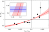 |
Fig. A.1. QPE intensity-recurrence relation. The ratio between the intensity of consecutive QPEs (in the 0.4-1 keV band) is shown as a function of the recurrence time between them, which is normalised to the average sum of consecutive long and short intervals (i.e. to the average separation between QPEs of the same type). The vertical dotted line separates short recurrence times from long ones, while the horizontal line separates weak-to-strong QPE pairs from strong-to-weak pairs. The best-fitting model is shown as a solid line and the 1σ uncertainty is represented by the shaded area. The inset in the upper left quadrant shows the intersection between the extrapolated model and the intensity ratio of the observed QPEs during XMM12. |
Here we assume that the correlation is valid in the whole interval  and that Ni /Ni + 1 = 1 when
  , as suggested by the data. Hence, we look for a model that satisfies the following constraints: (i) Ni /Ni + 1 → 0 when
  ; (ii) Ni /Ni + 1 → ∞ when
  ; (iii) Ni /Ni + 1 = 1 when
  . The simplest model that satisfies the above constraints is y = [x/(1−x)]α, where y = Ni/Ni + 1 and
  ; the best-fitting model is shown in Fig. A.1 as a solid line. We must point an important caveat: the best-fitting model is not only phenomenological, but is also based on a series of assumptions driven by the relatively few data points that populate Fig. A.1. We cannot exclude, for example, that had we detected more QPEs, the two empty quadrants in Fig. A.1 would have been populated as well, which would invalidate our conclusions below.
Although the statistical quality of the fit is poor (reduced  with α = 3.4 ± 0.8), and with the caveat expressed above, we can in principle derive Tsum from any measure of Ni/Ni + 1 and the corresponding
  between them. By extrapolating the best-fitting model to the observed Ni/Ni + 1 in the 0.4-1 keV band during XMM12 (see Table D.2), we derive
  ks. Although this estimate is obtained by extrapolating down to low
  a phenomenological model based on data in a significantly narrower range, the two independent estimates of
  derived from the QPO period and from the QPE intensity ratios (54 ± 4 ks and 52 ± 4 ks) are fully consistent with each other, which provides some support to the overall arguments.
Appendix B: QPE spectral properties
In order to study the spectral properties of the quiescent emission and QPEs at all epochs, we extracted EPIC pn quiescent and QPE X-ray spectra from all XMM-Newton observations with QPEs. The former are extracted from the whole exposures, QPEs excised, while the latter from time intervals of ≃ 1 ks centred on QPE peaks. There are two possible ways of interpreting QPE spectra. One can either assume that QPEs are an extra additive emission component superimposed on the otherwise stable disc emission, or that they represent the fast transient evolution of the disc emission itself.2 In either case, we are interested in deriving the properties of QPEs with respect to, and in comparison with, the quiescent state.
We first considered the additive scenario in which QPEs are superimposed on the quiescent emission, and we discuss the alternative point of view at the end of the section. We constructed QPE intrinsic (peak) X-ray spectra by subtracting the quiescence from QPEs, as in Miniutti et al. (2023). All spectra were grouped to a minimum of 20 counts per energy bin. We fitted jointly all QPE intrinsic spectra in the 0.3-1 keV band3 using χ2 minimisation in xspec and a simple spectral model comprising Galactic absorption (the Tbabs model in xspec) with NH fixed at 2.3 × 1020 cm−2 (HI4PI Collaboration et al. 2016), and a black body (at z = 0.0181) representing QPE peak emission, modified by extra intrinsic absorption (the zTbabs model in xspec). The latter is a simplified version of the warm absorber used by Miniutti et al. (2023) and it is chosen because the spectral quality of the QPE spectra prevented us from constraining the ionisation parameter well. We initially left the intrinsic absorber column density free to vary between the different observations. All column densities turned out to be consistent with each other with the exception of the XMM4 observation where no intrinsic absorption was preferred. However, by forcing all NH, z to be the same, the statistical quality of the fit was basically unaffected (χ2/ν = 666/704 versus χ2/ν = 661/700), so that we forced constant, observation-independent NH, z for simplicity, measuring NH, z = (2.8 ± 0.8)×1020 cm−2.
In Fig. B.1, we show the 0.2-2 keV X-ray luminosity of all QPE peaks as a function of their rest-frame temperature. As all spectra are super-soft, small differences in NH, z (or in the adopted absorption model) induce relatively large variations in the derived X-ray luminosities whose absolute values therefore should be taken with some caution. However, the trend shown in Fig. B.1 is preserved for any reasonable absorption model and parameters. QPEs during the previous regular phase (XMM3 to XMM5) as well as the stronger QPE in XMM12 have peak X-ray luminosity in the range of 2.8-4.2 × 1042 erg s−1 with a typical temperature of 90-100 eV, while QPEs during the irregular phase (XMM6) and the weak QPE in XMM12 peak at 1.1-1.5 × 1042 erg s−1 and are characterised by a lower peak temperature. The L-T correlation is shown in terms of the bolometric (black-body) luminosity in Fig. 5 (see Sect. 4 for a discussion).
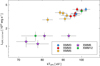 |
Fig. B.1. QPE-only LX-T relation. The 0.2-2 keV X-ray intrinsic peak luminosity of QPEs is shown as a function of rest-frame temperature. All spectra are quiescence-subtracted and they are described using an absorbed redshifted black-body model. |
We also considered the alternative scenario in which QPEs are not an additive emission component, but rather represent a transient and fast variation of the disc emission itself (or part of it). If so, the simplest way of describing QPEs is to consider the whole QPE X-ray spectrum (that is without subtracting the quiescence), modelling it with a single spectral component, as done for the quiescence. We then used the same spectral model for both QPE and quiescent spectra, namely a multi-temperature disc model (diskbb in xspec). We adopted the same absorption model (a simple redshifted neutral absorber), that is we neglected the warm absorber. All derived quiescent X-ray luminosities are therefore significantly lower than those presented in Miniutti et al. (2023) precisely because of the adopted absorption model. As mentioned, the relatively low quality of the QPE spectra (∼1 ks of exposure) prevented us from constraining the warm absorber properties during QPEs so that we preferred to use the simpler neutral absorber for both quiescence and QPEs, enabling us to compare the luminosity of the two states without introducing model-dependent uncertainties in the comparison. We note that the overall trend (luminosity versus temperature) discussed below is preserved for any chosen absorption model.
For clarity, we also point out that the QPE luminosity from non-quiescence-subtracted spectra is not exactly the sum of the quiescence and QPE-only spectra (the latter derived from quiescence-subtracted spectra). This is not surprising since the spectral model is different and thus extrapolates differently in the 0.2-2 keV band (data are only fitted in the 0.3-1 keV band). The QPE temperature is also slightly different because of the different spectral models describing QPEs and because of the slightly different spectral shape (spectra being either quiescence-subtracted or not). By re-fitting the non-quiescence-subtracted QPE spectra with a two-component model (a disc model for the quiescence and an additional black-body model for QPEs), we indeed recover the results for the QPE-only luminosity and temperature, as expected.
The resulting quiescent and QPE X-ray luminosity is shown in Fig B.2 for both the quiescence and QPEs as a function of (rest-frame) temperature. We also show best-fitting relations of the form LX ∝ Tq in both cases, and we derive qquiesc ≃ 4.1 (as noted by Miniutti et al. 2019, 2023), and qQPEs ≃ 0.9. As QPEs do not align onto the L ∝ T∼4 relation defined by the quiescent X-ray emission, QPEs and quiescence cannot be associated with disc emission from the same region. In other words, as already noted by Miniutti et al. (2019), QPEs are not produced by global mass accretion rate variation. This is also consistent with the lack of QPEs in the optical and UV and signals that only a very limited inner region on the disc is responsible for eruptions. Figure B.2 shows that QPEs must originate from a region with an area ∼6-30 times smaller than that responsible for the X-ray quiescent emission (if eruptions are black body-like, as the data indicate). Assuming that the quiescent X-ray emission region has radius Rquiesc ≃ 20 Rg (Rg = GMBH/c2) this means that QPE emission is confined within radii of the order of ∼3.5-8 Rg. The flat qQPEs implies that the hottest (and most luminous) QPEs are associated with the smallest emitting regions. A very small QPE emitting region could in principle be consistent with disc instabilities and a very small inner unstable region (see e.g. Śniegowska et al. 2023; Pan et al. 2023), with mass injection at small radii producing a burst in mass accretion rate limited to the inner annulii (possibly as in King 2020, 2022; Chen et al. 2022; Wang et al. 2022) or with the transient formation of an inner, optically thick, warm corona inducing the emergence of a transient soft X-ray excess (as discussed by Miniutti et al. 2019).
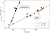 |
Fig. B.2. Total QPE and quiescent emission LX-T relation. The 0.2-2 keV X-ray luminosity is shown as a function of rest-frame temperature. The squares denote results from fits to the quiescent spectra only; the circles are from fits to the QPE spectra (not quiescence-subtracted). The same colour scheme as in Fig. B.1 is adopted, and black data points denote observations with no QPEs. All spectra are described using the same absorbed redshifted disc model (diskbb). The dashed (dotted) lines are best-fitting relations for the quiescence (QPEs) of the form LX ∝ Tq resulting in qquiesc ≃ 4.1 and qQPEs ≃ 0.9. |
Appendix C: Ability to detect QPEs
Figures B.1 and B.2 suggest that QPEs can be identified efficiently by their different temperatures with respect to the quiescent level and by the correlation between (peak) luminosity and temperature. Since QPEs in GSN 069 only carry a small fraction of the quiescence bolometric luminosity, QPEs with peak temperature kTQPE close to that of the quiescent emission kTquiesc cannot be efficiently detected against it as they would appear as relatively low-amplitude fluctuations of the quiescent level with no striking energy dependence. In Fig. C.1, we show the relative QPE amplitude in the 0.2-2 keV as a function of the ratio of QPE to quiescent temperature. We take the QPE temperatures from fits to the quiescence-subtracted QPE spectra, but we note that Fig. C.1 is qualitatively very similar when considering fits to the full QPE spectra (i.e. without subtracting the quiescence). Hence, our conclusions below are general and do not depend on whether QPEs are superimposed on the disc emission or represent instead a transient evolution of the disc emission itself.
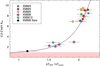 |
Fig. C.1. Dependence of QPE detection on the eruptions-to-quiescence temperature ratio. The relative 0.2-2 keV QPE amplitude is shown as a function of the ratio of QPE to quiescent temperatures. The horizontal shaded area denotes the region below the QPE detection threshold. Also shown (black data point) is the strongest X-ray flare seen in any observation with no clearly detected QPEs. The dotted line shows a simple fit to the data, whose functional form is chosen so that Arel = 1 when kTQPE/kTquiesc = 1 (see text for details). |
The QPE relative amplitude is defined as Arel = CQPE/Cquiesc, where CQPE and Cquiesc are the (total) QPE and quiescent 0.2-2 keV count rates respectively. The relative amplitude is energy-dependent. As an example, the highest amplitude in the 0.2-2 keV band is Arel, max ≃ 9.5, increasing to ≃82 in the 0.6-2 keV band, mostly because of the much lower contribution of the quiescent emission in higher energy bands. The dotted line in Fig. C.1 shows a (non-unique) best-fitting model of the form y = (ax + bxq)/(a + b), chosen so that Arel = 1 when kTQPE/kTquiesc = 1. The shaded area in Fig. C.1 denotes the region below the QPE detection threshold.
The trend in Fig. C.1, as well as its best-fitting model, suggest that the detection of QPEs with kTQPE/kTquiesc ≲ 1.2 is already challenging in GSN 069. The black data point in Fig. C.1 refers to the brightest X-ray flare observed in any of the observations with no clear QPEs, namely the best QPE candidate from the XMM2 and the XMM7 to XMM11 observations. The light curve from the corresponding observation (XMM8) is shown in Fig. C.2 where the QPE candidate is highlighted with filled circles. As shown in Fig. C.1, we cannot exclude that the XMM8 flare is in fact a weak QPE with very little temperature contrast with respect to the quiescent emission.
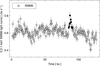 |
Fig. C.2. Best QPE candidate in QPE-less observations. We show the 0.2-1 keV light curve from the XMM8 observation. The most prominent flare, that is the best QPE candidate from all high-luminosity observations with no unambiguous QPEs, is highlighted. We used here a time bin of 600 s. The flare spectrum used to derived the quantities in Fig. C.1 (count rate and peak temperature) was extracted from a ∼1 ks time-interval around the peak. The empty circles define the period during which we accumulated the quiescent spectrum. |
Hence, a question arises of whether QPEs with similar properties as those observed during the XMM3 to XMM6 observations could also be present in the high-luminosity XMM2 and XMM7 to XMM11 observations, but be undetected against a higher flux and higher temperature quiescent emission. To answer this question, we selected a set of representative QPEs, and we studied how they would have appeared in observations when the quiescent emission was similar to that during the high-luminosity QPE-less observations. We considered the XMM12 QPEs as representative of QPEs in the previous regular phase (the strong QPE in XMM12) and of the weaker ones in the irregular phase (the weak QPE in XMM12), as shown in Fig. C.1. We also considered the irregular, weaker QPEs of the XMM6 observation for completeness. In this case, in order to estimate the appearance of standard QPEs in observations when the quiescent emission was brighter, we had to assume the additive nature of QPEs, and we then proceeded as follows: from the quiescence-subtracted peak QPE spectra, we recorded the QPE-only 0.2-2 keV count rate CQPE − only and peak temperature kTQPE. We then considered the quiescent spectra of all observations with no QPEs (XMM2 and XMM7 to XMM11). Since these observations all have similar luminosities and temperatures (see Miniutti et al. 2023, Fig. 9), we estimated the average 0.2-2 keV quiescent count rate Cquiesc and temperature kTquiesc, and we computed the relative QPE amplitude Arel = (CQPE − only+Cquiesc)/Cquiesc and temperature ratio kTQPE/kTquiesc for the selected QPEs.
Figure C.3 shows the resulting Arel as a function of the temperature ratio, which is how these QPEs would have appeared in observations during which the quiescent level was equal to the average emission (in both flux and temperature) in observations with no QPEs, under the assumption that QPEs are an extra emission component superimposed on the quiescent (disc) emission. Although both Arel and kTQPE/kTquiesc are slightly reduced due to higher Cquiesc and kTquiesc (compare Fig. C.3 with Fig. C.1), both the strong QPE in XMM12 (representative of all QPEs during the previous regular phase) and the weak QPE (as well as all irregular QPEs during XMM6) lie well above the detection threshold. We can therefore safely conclude that the lack of clear QPEs in the high quiescent luminosity observations is not due to the higher flux and temperature of the quiescent emission, but instead is intrinsic. In other words, if QPEs are present during these observations (XMM2 and XMM7 to XMM11), they must be significantly colder than any of the detected QPEs with kTQPE/kTquiesc ≲ 1.
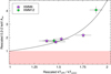 |
Fig. C.3. Estimated QPE appearance during observations with no clear QPEs (XMM2 and XMM7 to XMM11). Shown is the relative 0.2-2 keV QPE amplitude as a function of the ratio of QPE to quiescent temperatures for the XMM6 and XMM12 observations. Arel and kTQPE/kTquiesc have been rescaled to show how additive QPEs would have appeared during high-luminosity observations with no unambiguous QPEs (see text for details). The dotted line shows a simple fit to the data of the same form as that used for Fig. C.1. |
Appendix D: Tables
Summary of the XMM-Newton and Chandra pointed observations of GSN 069.
Baseline best-fitting parameters for the 0.4-1 keV and 0.2-1 keV EPIC-pn light curves from the XMM12 observation.
Baseline plus sine function best-fitting parameters for the re-binned 0.2-1 keV EPIC-pn light curves from the XMM12 observation.
All Tables
Baseline best-fitting parameters for the 0.4-1 keV and 0.2-1 keV EPIC-pn light curves from the XMM12 observation.
Baseline plus sine function best-fitting parameters for the re-binned 0.2-1 keV EPIC-pn light curves from the XMM12 observation.
All Figures
|
Fig. 1. EPIC light curves from the XMM12 observation. Light curves in the 0.2 − 1 keV with time bins of 200 s (pn) and 400 s (MOS) are shown. Background light curves, rescaled to the same extraction area, are also shown to highlight the slightly higher background during the initial ∼10 ks of the EPIC exposures. The start of the MOS 1 exposure is taken as origin for the time-axis in all cases. |
| In the text | |
|
Fig. 2. Quiescent level QPO. Upper panel: 0.2–1 keV pn light curve with time bins of 1000 s, together with its baseline best-fitting model. Middle panel: Resulting residuals and, as a solid line, a sine function that is plotted to guide the eye. Lower panel: Residuals once the original light curve is fitted by adding a sine function to the baseline model. |
| In the text | |
|
Fig. 3. Comparison between old and new QPE phases. Upper panel: Typical model light curve for observations during the old regular QPE phase. Lower panel: Qualitative representation of the light curve from the XMM12 observation (new QPE phase; solid line) and one possible extrapolation of longer-term behaviour based on the arguments discussed in Sect. 3 and Appendix A (dashed line). The light curves were normalised so that the intensity of the strong QPEs is the same in both panels. The same quiescent level is assumed for visual clarity. |
| In the text | |
|
Fig. 4. Quiescent luminosity long-term evolution. Shown is the Lbol evolution of the quiescent emission over the past ∼12 yr. The dotted-solid line is a possible model discussed in Miniutti et al. (2023). The grey data points refer to observations that are too short to ensure the detection of QPEs (squares for Swift and circles for XMM-Newton data). Coloured and black data points represent instead long enough observations respectively with and without QPEs. The purple star denotes the XMM6 observation with irregular QPEs. A Chandra observation (exhibiting three QPEs) performed between the XMM4 and XMM5 observations was omitted as the corresponding quiescent luminosity is highly uncertain (see Table D.1). |
| In the text | |
|
Fig. 5. QPE Lbol–T relation. The QPE-only Lbol is shown as a function of QPE rest-frame temperature from quiescence-subtracted QPE spectra assuming a simple absorbed black-body model. The dotted lines show Lbol ∝ T4 relations with different normalisation. The actual best-fitting relation is somewhat shallower with index ≃3.1. |
| In the text | |
|
Fig. A.1. QPE intensity-recurrence relation. The ratio between the intensity of consecutive QPEs (in the 0.4-1 keV band) is shown as a function of the recurrence time between them, which is normalised to the average sum of consecutive long and short intervals (i.e. to the average separation between QPEs of the same type). The vertical dotted line separates short recurrence times from long ones, while the horizontal line separates weak-to-strong QPE pairs from strong-to-weak pairs. The best-fitting model is shown as a solid line and the 1σ uncertainty is represented by the shaded area. The inset in the upper left quadrant shows the intersection between the extrapolated model and the intensity ratio of the observed QPEs during XMM12. |
| In the text | |
|
Fig. B.1. QPE-only LX-T relation. The 0.2-2 keV X-ray intrinsic peak luminosity of QPEs is shown as a function of rest-frame temperature. All spectra are quiescence-subtracted and they are described using an absorbed redshifted black-body model. |
| In the text | |
|
Fig. B.2. Total QPE and quiescent emission LX-T relation. The 0.2-2 keV X-ray luminosity is shown as a function of rest-frame temperature. The squares denote results from fits to the quiescent spectra only; the circles are from fits to the QPE spectra (not quiescence-subtracted). The same colour scheme as in Fig. B.1 is adopted, and black data points denote observations with no QPEs. All spectra are described using the same absorbed redshifted disc model (diskbb). The dashed (dotted) lines are best-fitting relations for the quiescence (QPEs) of the form LX ∝ Tq resulting in qquiesc ≃ 4.1 and qQPEs ≃ 0.9. |
| In the text | |
|
Fig. C.1. Dependence of QPE detection on the eruptions-to-quiescence temperature ratio. The relative 0.2-2 keV QPE amplitude is shown as a function of the ratio of QPE to quiescent temperatures. The horizontal shaded area denotes the region below the QPE detection threshold. Also shown (black data point) is the strongest X-ray flare seen in any observation with no clearly detected QPEs. The dotted line shows a simple fit to the data, whose functional form is chosen so that Arel = 1 when kTQPE/kTquiesc = 1 (see text for details). |
| In the text | |
|
Fig. C.2. Best QPE candidate in QPE-less observations. We show the 0.2-1 keV light curve from the XMM8 observation. The most prominent flare, that is the best QPE candidate from all high-luminosity observations with no unambiguous QPEs, is highlighted. We used here a time bin of 600 s. The flare spectrum used to derived the quantities in Fig. C.1 (count rate and peak temperature) was extracted from a ∼1 ks time-interval around the peak. The empty circles define the period during which we accumulated the quiescent spectrum. |
| In the text | |
|
Fig. C.3. Estimated QPE appearance during observations with no clear QPEs (XMM2 and XMM7 to XMM11). Shown is the relative 0.2-2 keV QPE amplitude as a function of the ratio of QPE to quiescent temperatures for the XMM6 and XMM12 observations. Arel and kTQPE/kTquiesc have been rescaled to show how additive QPEs would have appeared during high-luminosity observations with no unambiguous QPEs (see text for details). The dotted line shows a simple fit to the data of the same form as that used for Fig. C.1. |
| In the text | |
Current usage metrics show cumulative count of Article Views (full-text article views including HTML views, PDF and ePub downloads, according to the available data) and Abstracts Views on Vision4Press platform.
Data correspond to usage on the plateform after 2015. The current usage metrics is available 48-96 hours after online publication and is updated daily on week days.
Initial download of the metrics may take a while.