| Issue |
A&A
Volume 693, January 2025
|
|
|---|---|---|
| Article Number | A150 | |
| Number of page(s) | 17 | |
| Section | Extragalactic astronomy | |
| DOI | https://doi.org/10.1051/0004-6361/202451980 | |
| Published online | 13 January 2025 | |
Direct-method metallicity gradients derived from spectral stacking with SDSS-IV MaNGA
1
Dipartimento di Fisica e Astronomia, Università di Bologna, Via Gobetti 93/2, I-40129 Bologna, Italy
2
INAF, Astrophysics and Space Science Observatory Bologna, Via P. Gobetti 93/3, I-40129 Bologna, Italy
3
INAF-Osservatorio Astronomico di Padova, vicolo dell’Osservatorio 5, 35122 Padova, Italy
4
INAF - Osservatorio Astrofisico di Arcetri, Largo E. Fermi 5, 50125 Firenze, Italy
⋆ Corresponding author; This email address is being protected from spambots. You need JavaScript enabled to view it.
Received:
24
August
2024
Accepted:
12
November
2024
Abstract
Chemical abundances are key tracers of the cycle of baryons that drives the evolution of galaxies. Most measurements of interstellar medium abundances and metallicity gradients in galaxies are, however, based on model-dependent strong-line methods. Direct chemical abundances can be obtained via the detection of weak auroral lines, but such lines are too faint to be detected by large spectroscopic surveys of the local Universe. In this work we overcome this limitation and obtain metallicity gradients from direct-method abundances by stacking spectra from the MaNGA integral field spectroscopy survey. In particular, we stacked 4140 star-forming galaxies across the star formation rate–stellar mass plane and across six radial bins. We calculated electron temperatures for [OII], [SII], [NII], [SIII], and [OIII] across the majority of the stacks. We find that T[OII] ≈ T[SII] ≈ T[OII], as expected since these ions all trace the low-ionization zone of nebulae. The [OIII] temperatures become substantially higher than those of other ions at high metallicities, indicating potentially unaccounted for spectral contamination or additional physics. In light of this uncertainty, we based our abundance calculation on the temperatures of [SIII] and the low-ionization ions. We recover a mass-metallicity relation similar to that obtained with different empirical calibrations. We do not, however, find evidence of a secondary dependence on the star formation rate using direct metallicities. Finally, we derive metallicity gradients that become steeper with stellar mass for log(M⋆/M⊙) < 10.5. At higher masses, the gradients flatten again, confirming with auroral line determinations the trends previously defined with strong-line calibrators.
Key words: galaxies: abundances / galaxies: evolution / galaxies: ISM / galaxies: star formation
© The Authors 2025
 Open Access article, published by EDP Sciences, under the terms of the Creative Commons Attribution License (https://creativecommons.org/licenses/by/4.0), which permits unrestricted use, distribution, and reproduction in any medium, provided the original work is properly cited.
This article is published in open access under the Subscribe to Open model. This email address is being protected from spambots. You need JavaScript enabled to view it. to support open access publication.
1. Introduction
Studying the abundance of heavy elements within the interstellar medium (ISM) of galaxies offers valuable insights into the physical mechanisms driving galaxy formation and evolution (Tinsley 1980; Rafelski et al. 2012). The continuous inflow and outflow of baryonic matter within galaxies determine key galactic properties, linking the stellar mass (M⋆), star formation rate (SFR), and metal content. Consequently, scaling relations such as the mass-metallicity relation (MZR; Tremonti et al. 2004; Kewley & Ellison 2008; Maiolino et al. 2008; Zahid et al. 2014; Sanders et al. 2015; Jones et al. 2020; Nakajima et al. 2023) and the M⋆–metallicity-SFR relation, also known as the fundamental metallicity relation (FMR; Mannucci et al. 2010; Bothwell et al. 2013; Nakajima & Ouchi 2014; Curti et al. 2020a, 2024), play pivotal roles as observational benchmarks in the development of galaxy evolution models.
Moreover, the chemical evolution of the ISM serves as a probe of the timescale for the assembly of galaxy discs (Pagel 1997; Spolaor et al. 2010; Rafelski et al. 2012; Maiolino & Mannucci 2019). Models describing galactic metallicity gradients, for example, generally support the inside-out scenario for the growth of galactic disks (Larson 1976; Matteucci & Francois 1989; Boissier & Prantzos 1999; Pezzulli & Fraternali 2016). Disagreements between the different models persist at higher redshifts, where gradients are predicted to become shallower or steeper depending on the strength of feedback and the outflow properties (e.g., Chiappini et al. 2001; Mott et al. 2013; Prantzos & Boissier 2000; Pilkington et al. 2012; Henriques et al. 2020; Sharda et al. 2021). Recent integral field spectroscopy (IFS) observations of nearby galaxies (e.g., Rosales-Ortega et al. 2011; Croom et al. 2012; Sánchez et al. 2014; Ho et al. 2015; Bryant et al. 2015; Sánchez-Menguiano et al. 2016) have provided a comprehensive view of metallicity gradients in the local Universe, with extensions to high redshifts currently being pursued with near-IR instruments, such as K-band Multi Object Spectrograph (KMOS) or NIRSpec on JWST.
These gradients have been derived using empirical calibrations or theoretical models, in the local Universe (e.g., Sánchez et al. 2014; Pilyugin et al. 2015; Belfiore et al. 2017; Poetrodjojo et al. 2018; Berg et al. 2020; Mingozzi et al. 2020) and at higher redshifts (e.g., Curti et al. 2020b; Wang et al. 2020, 2022; Simons et al. 2021; Li et al. 2022; Venturi et al. 2024; Cheng et al. 2024), with notably smaller sample sizes. They generally align with models grounded in the conventional inside-out framework of disk formation, which forecast a rapid self-enrichment process leading to elevated oxygen abundances and mostly negative metallicity gradients, especially when normalized to the optical size of the galaxy. Despite the good agreement between simulations and observations in the local Universe, their divergent behavior at higher redshifts remains an open question. Simulations like IllustrisTNG and FIRE (e.g., Ma et al. 2017; Hemler et al. 2021) as well as some observations (e.g., Ju et al. 2024) show that at z ≳ 1, massive galaxies typically exhibit steeper negative metallicity gradients. However, several observations of high-redshift galaxies reveal a larger fraction of flat or inverted metallicity gradients compared to their local counterparts (e.g., Curti et al. 2020a; Simons et al. 2021; Cheng et al. 2024).
The conflicting outcomes at low and high redshifts observed in certain earlier studies may be attributed to limited sample sizes and variations in the strong-line diagnostics employed to measure metallicity gradients. Utilizing diverse metallicity diagnostics can introduce substantial systematic errors (see Kewley & Ellison 2008; Ellison et al. 2008; López-Sánchez et al. 2012). For instance, the observed flattening in metallicity gradients toward the central regions of the largest spiral galaxies, as discussed in Zinchenko et al. (2016), could be attributed to contamination from emission from other ionizing sources, such as the low-ionization nuclear emission line regions found in massive galaxies (Belfiore et al. 2016), potentially affecting the reliability of strong-line diagnostics. Alternatively, in extremely metal-rich central areas, metallicity levels may be approaching a saturation point, nearing their maximum attainable theoretical yield (e.g., Belfiore et al. 2017).
Furthermore, the relation between metallicity gradients and the stellar mass of the galaxy, known as the mass–metallicity gradient relation (MZGR), can trace the disk assembly process (Maiolino & Mannucci 2019). Sánchez et al. (2014) and Ho et al. (2015) demonstrate that normalizing radii to the galaxy effective radius (Re) reduces the significant dispersion in metallicity gradients.
Using Mapping Nearby Galaxies at APO (MaNGA) Data Release (DR) 13 data, Belfiore et al. (2017) found a nonlinear dependence of the metallicity gradient on the stellar mass (109 − 1011 M⊙). Poetrodjojo et al. (2018) subsequently independently confirmed the changes in the metallicity gradient with stellar mass, using data from the SAMI (Bryant et al. 2015) in the stellar mass range 109 − 1010.5 M⊙. These findings offer essential new constraints for chemical evolution models and their integration into hydrodynamical simulations, particularly regarding the balance between feedback strength and wind recycling in different mass regimes.
Observationally, especially at subsolar metallicities, the most precise approach for determining the oxygen abundance in the gas phase involves determining the effective temperature (Te) within H II regions, a method commonly referred to as the Te technique or the “direct method” (Pagel et al. 1992; Izotov et al. 2006). This method hinges on the detection of faint auroral lines, which are not detected in individual objects in large spectroscopic surveys such as MaNGA or SAMI.
The primary goal of this work is to directly measure the gas-phase metallicity gradients based on electron temperatures extracted from auroral lines across a representative set of galaxies in the local Universe. We achieved this by stacking spectra of galaxies we expect to have similar metallicities. In particular, we stacked the spectra of galaxies in bins in the M⋆–SFR plane since these two physical parameters are the main predictors of metallicity according to the FMR (e.g., Mannucci et al. 2010; Andrews & Martini 2013; Nakajima & Ouchi 2014). We used data from the MaNGA survey (DR17; Abdurro’uf et al. 2022), making our study the first of its kind to analyze the Te metallicity gradient across the entire mass range of 108.4–1011.2 M⊙.
The paper is organized as follows: In Sect. 2 we present the galaxy sample obtained from the MaNGA survey. Section 3 outlines the methodology and our abundance determinations. Section 4 presents the results, which are discussed in Sect. 5. Finally, Sect. 6 summarizes the conclusions of this study. We assume a Λ cold dark matter cosmology with H0 = 70 km s−1 Mpc−1, Ωm = 0.3, and ΩΛ = 0.7.
2. Data
2.1. The MaNGA data
The fourth-generation Sloan Digital Sky Survey (SDSS) MaNGA project used IFS to study the ionized ISM and stellar populations of a statistical sample of local galaxies at kiloparsec scales. MaNGA DR17 includes observations of more than 10 000 local galaxies, in the redshift range 0.002 < z < 0.15 (Fig. 1). MaNGA used integral field units composed of hexagonally packed fiber bundles of different sizes for scientific observations (from 19 to 127 fibers). In addition, the MaNGA instrument suite consisted of 92 single fibers for sky subtraction and a set of 12 seven-fiber mini-bundles for flux calibration (Yan et al. 2016). All fibers were fed into the dual beam BOSS spectrographs, which have a spectral resolution of R ≃ 2000 and span the wavelength range 3600–10 300Å (Smee et al. 2013).
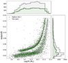 |
Fig. 1. Redshift–M⋆ plane of the MaNGA sample utilized in this study. The star-forming galaxies (see Sect. 2.1) chosen for the study of gas-phase metallicity are shown in green and the entire MaNGA DR17 sample in gray. The redshift and stellar mass distributions for the selected and full samples used in this work are shown as green and gray histograms. |
MaNGA offers spatially resolved spectra that span a radial range up to 1.5 times the Re for the primary sample, which accounts for approximately two-thirds of the total sample. For the secondary sample, constituting roughly one-third of the total and located at a slightly higher redshift, the spatially resolved spectra extend to 2.5 Re (Law et al. 2015; Wake et al. 2017). MaNGA DR17 data were reduced using the MaNGA reduction pipeline version v3_1_1, as detailed in Law et al. (2021, 2016).
In this work we used the resulting reduced datacubes, with a pixel size of 0.5″. The typical point spread function for the MaNGA datacubes is estimated to have a median full width at half maximum of 2.5″. This corresponds to ∼1.5 kpc at the median distance of the MaNGA sample.
The MaNGA Data Analysis Pipeline (DAP; Belfiore et al. 2019; Westfall et al. 2019) performed spectral fitting for the determination of the stellar and gas kinematics, as well as the fluxes of various emission lines. The DAP workflow employed adaptive Voronoi spatial binning (Cappellari & Copin 2003) to achieve a minimum target signal-to-noise ratio (S/N) of around 10 in the stellar continuum. After conducting measurements of stellar kinematics, it derived emission line fluxes using the full spectral fitting code pPXF (Cappellari & Emsellem 2004; Cappellari 2017). For DR17 DAP employed the MILES stellar library (Sánchez-Blázquez et al. 2006) to extract stellar kinematics, while for modeling the stellar continuum within the emission line module it employed a subset of MaNGA Stellar Library Simple Stellar Population models (MaStar SSP, Maraston et al. 2020) derived from the MaStar stellar library (Yan et al. 2019). In this work we employed the integrated emission line fluxes reported in DAP v3_1_1 catalog to select a sample of star-forming galaxies from the full MaNGA sample. We also employed line fluxes and velocities from the emission lines maps released as part of DR17 to perform a selection of spaxels and to de-redshift the spectra before stacking.
We adopted the integrated stellar masses estimates from the extended NSA targeting catalog (Blanton et al. 2011). These were obtained from fitting the SDSS imaging data and adopting the Chabrier (2003) initial mass function. The global SFR for each galaxy is obtained from its dust-corrected Hα luminosity, using the line fluxes from the integrated DAP catalog, and adopting the conversion factor in Hao et al. (2011). While discrepancies in the apertures used for stellar mass and SFR measurements may introduce some scatter, Belfiore et al. (2018) found that aperture effects play a fairly minor role. In particular, they compared masses derived from within the MaNGA bundle and from integrated photometry and SFR measured within 1.5 Re and 2.5 Re, finding median offsets < 0.05 dex.
Finally, we calculated deprojected galactocentric radii using the semi-axis ratio (b/a) from the MaNGA NSA catalog obtained via elliptical Petrosian analysis. Using the semi-axis ratio, the galaxy inclination (i) was computed assuming constant oblateness q = 0.13 (Giovanelli et al. 1994) using
 (1)
(1)
The NSA elliptical Petrosian effective radius, Re, in the r band was used as a normalizing scale-length for deriving gradients.
To measure metallicity gradients, we selected a subsample of star-forming galaxies from the full MaNGA dataset. In particular, we selected galaxies that are classified as star-forming based on Baldwin, Phillips, and Terlevich (BPT) diagrams (Baldwin et al. 1981) and using the fluxes extracted from their integrated spectra, as reported in MaNGA DAP catalog.
Galaxies were classified as star-forming if they lie below the Kauffmann et al. (2003) demarcation line criteria in the [O III]λ5007/Hβ versus [N II]λ6583/Hα diagram and the Kewley et al. (2001) line in the [O III]λ5007/Hβ versus [S II]λλ6716,6731/Hα diagram. We have 4748 galaxies that meet these criteria; they span the stellar mass range 8.4 < log(M⋆/M⊙) < 11.5. We note that this represents the number of star-forming galaxies in MaNGA sample, and while our binning captures the majority, not all of them are included in the SFR − M⋆ bins (see Sect. 2.2).
2.2. Stacking procedure
We aim to measure weak auroral lines in spectral stacks. Our approach consists in stacking in radial bins and across galaxy properties that select galaxies with similar metallicities. Assuming that a galaxy’s integrated metallicity is described by the FMR, we bin galaxies across the M⋆ and SFR plane.
We defined 56 bins in the SFR–M⋆ plane (Fig. 2), with 12 bins in stellar mass and a variable number (up to seven) bins in SFR. This binning scheme includes 4140 star-forming galaxies, excluding approximately 13% of the sample, which lies outside these bins. The bins span log(M⋆/M⊙) = [8.4–11.5] and log(SFR) ∼ −2.0 to +1.0 with an average continuum S/N of 37.5 at ∼ 5000 Å. The number of galaxies in each bin ranges from 1 to 211, with an average of 45 galaxies per bin. We tested various alternative binning configurations in this space, but found that the current one is the best compromise between the width of the bins and the ability to detect auroral lines.
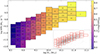 |
Fig. 2. Position of the bins used for spectral stacking in this work in the SFR–M⋆ plane. Each rectangle represents a bin, color-coded according to its median strong-line metallicity using the Pettini & Pagel (2004) calibration and extinction-corrected emission lines from the MaNGA DAP catalog. The number of galaxies in each bin is reported. In the inset in the lower right, our stacking grid is shown superimposed on the distribution of individual MaNGA star-forming galaxies in the SFR–M⋆ plane. The integrated spectra, global and radially binned, are available online (see Tables B.2 and B.1). |
Before stacking the spectra, we corrected for their velocity shifts by using the MaNGA velocity map and the systemic redshift of the galaxy, shifting each spaxel’s spectral data to its rest-frame wavelength. We also applied an extinction correction to the stacked spectra of individual galaxies. This correction used the extinction curve of O’Donnell (1994), assuming an intrinsic Balmer decrement of Hα/Hβ = 2.86. The Hα and Hβ values were determined by modeling the stellar continuum and emission lines, as described in Sect. 3.1. Consequently, we utilized the reddening-corrected spectra of individual galaxies within each SFR–M⋆ bin to generate the final stacked (averaged) spectra for each respective bin. To derive “integrated” abundances, spaxels were considered up to the radius covered by all samples, which is 1.5 Re, and in the spatially resolved context, the analysis was conducted within different radial bins, as mentioned below.
Using extinction-corrected emission lines, the global strong-line metallicity of each galaxy was determined using the empirical calibration introduced by Pettini & Pagel (2004). The median metallicity of each bin, represented by the bin’s color code in Fig. 2, reflects the average metallicity within that bin. The standard deviation of metallicity values in each bin is small, 0.07 dex on average.
For spatially resolved analysis, we stacked spectra of galaxies in different radial bins. Binning radially is a compromise between maintaining a sufficient number of spaxels to guarantee the detection of auroral lines and having a meaningful number of radial bins to determine the shape the gradient. For each bin in the M⋆-SFR plane, we drew a set of radial bins. We experimented with equidistant radial bins, but eventually converged on a set of radial bins that more closely achieve a fixed S/N. The bins we defined have boundaries at 0.0, 0.35, 0.65, 0.85, 1.1, 1.5, and 2.5 Re. Therefore, we constructed six radial stacks for each bin in the SFR–M⋆ plane.
In our stacking analysis we exclusively incorporated spaxels that meet the star-forming classification criteria defined by the BPT method cuts discussed above for integrated galaxies. For spaxels, we used the line maps obtained using the MaNGA DAP. Spaxels with flagged Hα velocity or flux measurements were omitted from the stacks.
3. Data analysis
3.1. Spectral fitting
We performed spectral fitting of the stacked spectra using pPXF (Cappellari 2017) and modeled the continuum with 32 EMILES simple stellar population templates (Vazdekis et al. 2016). These models were generated using the initial mass function by Chabrier (2003), BaSTI isochrones (Pietrinferni et al. 2004), eight ages ranging from 0.15 to 14 Gyr (logarithmically spaced in steps of 0.22 dex), and four metallicities, [Z/H] = [–1.5, –0.35, 0.06, 0.4]. During the fit we employed sixth-degree multiplicative polynomials.
We modeled the spectrum in different spectral windows (see Fig. 3) approximately 200 Å wide, where the velocity dispersion of emission lines are tied to the strongest line’s σv in each window (Table 1). This procedure was found to produce smaller residuals than performing the pPXF fit over the entire wavelength range. We imposed a few additional constraints in the process of line fitting. In the case of the [OIII]λ4959,5007 and [NII]λ6548,6583 doublets, the dispersion of the individual components of the doublet was fixed and their amplitude ratios were set to the ratios of the relative Einstein coefficients. For [SIII] we only modeled the [SIII]λ9068 emission line since the [SIII]λ9530 line is either highly contaminated by the sky emission or, for galaxies at z > 0.08, falls outside the MaNGA wavelength range. Furthermore, we masked all spectra in the range 5887–5903 Å to avoid any potential residuals from the strong sky line at λ5894.6 Å, which may overlap with the [N II]λ5754 emission line in the redshift range 0.022 < z < 0.026. As a result, the [NII]λ5754 is masked for ∼8% of our galaxy sample.
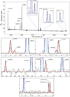 |
Fig. 3. Topmost panel: Stacked spectrum of a SFR–M⋆ bin (M⋆ = 108.65 M⊙ and SFR = 1−1.3 M⊙ yr−1), showing zoomed-in views of the spectral fits around some of the strong nebular lines. In the subplots below we zoom in on the fit residuals in specific spectral regions to highlight the detection of faint, temperature-sensitive auroral lines (in red) and other nearby emission lines (blue). The dashed green lines represent the standard deviation of residual fits in each wavelength window. The emission line fluxes and associated uncertainties, global and radially binned, are available online (see Tables B.3 and B.4). |
All emission lines measured in this study.
pPXF estimates its formal uncertainties from the covariance matrix of the standard errors in the fitted parameters, which may lead to underestimations in the parameter uncertainties. To determine a more realistic flux error, we multiplied the formal pPXF flux error by the ratio of the modeled residual standard deviation over the median flux error in each wavelength window. This process effectively rescales the flux uncertainties to match those of the fit residuals, therefore taking the errors introduced by imperfect continuum subtraction into account.
3.2. Spectral contamination of the [OIII]λ4363 emission line
We find at least one emission feature between 4358 Å and 4362 Å that is blended with the [O III]λ4363 auroral line, more commonly in the high metallicity stacks. Such contamination of the [OIII]λ4363 line has previously been reported in the literature (Andrews & Martini 2013; Curti et al. 2017). Although the exact nature of this feature is unknown, it is at least in part constituted by the [Fe II]λ4360 emission line (see Fig. 4).
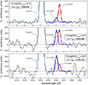 |
Fig. 4. Spectral residuals in the wavelength range near the [O III]λ4363 line, after stellar continuum subtraction. The red and blue Gaussian fits represent [O III]λ4363 and [Fe II]λ4360 emission lines, respectively. The dashed lines illustrate the standard deviation of residual fits in the corresponding windows. The strong-line metallicity and measured [O III] temperature of each stack are reported in the panels. The contamination of the [O III]λ4363 line becomes more relevant with increasing metallicity. |
To mitigate the influence of [Fe II]λ4360 contamination during fitting, we set its flux to 0.73× that of the nearby, isolated [Fe II]λ4288 line. This ratio follows that of the corresponding Einstein coefficient since both lines originate from the same atomic upper level. We also simultaneously fit the features around 4363 Å by linking their velocity widths and central wavelengths to Hγ. The various components of the fit are shown in Fig. 4 for three SFR–M⋆ bins with different strong-line metallicities.
3.3. Density and temperature measurements
To measure electron densities we used the PyNeb software package (Luridiana et al. 2012, 2015) and the [S II]λ6717,6731 doublet ratio. The majority of our stacks have low electron densities (ne ≤ 100 cm−3) since the detected [S II] ratios are usually close to the theoretical limit of 1.41 with σ ∼ 0.12. Therefore, we set ne to 100 cm−3 for all bins, which is the typical electron density in HII regions (Osterbrock 1989). The use of a lower density value does not affect the inferred temperatures.
We inferred electron temperatures using PyNeb, and temperature-sensitive auroral-to-nebular ratios. To determine the temperatures of low-ionized atoms, we used the [OII]λλ7318, 7319, 7329, 7330/[OII]λλ3726, 3728 ratio for [OII], the [SII]λλ4068, 4076/[SII]λλ6716, 6730 ratio for [SII], and the [NII]λ5754/[NII]λ6583 ratio for [NII]. We used the [OIII]λ4363/[OIII]λ5006 ratio to obtain [OIII] temperatures, which traces the high-ionization zone, and the [SIII]λ6312/[SIII]λλ9068, 9530 ratio for [SIII] temperature, which traces the intermediate-ionization zone. To derive uncertainties, we added random Gaussian noise consistent with the flux uncertainties and ran 1000 Monte Carlo (MC) realizations to obtain the best-fit temperature and its uncertainty, the latter taken as standard deviation of the distribution. The temperature with uncertainties below 500 K are considered reliable for determining ionic abundances.
To compare with the abundances obtained via the “direct” method, we also computed strong-line metallicity estimates for each bins based on strong nebular lines. We used as a fiducial estimate the one obtained from Pettini & Pagel (2004), P04 hereafter, based on the O3N2 index, defined as O3N2 ≡ log(([O III]λ5007/Hβ)/([N II]/Hα)). The O3N2 index offers the advantage of reducing uncertainties stemming from flux calibration or extinction correction issues, as it relies on line ratios with similar wavelengths that vary monotonically with metallicity. The uncertainties in the strong-line estimates of metallicity are also estimated via MC simulations.
In Fig. 5, the temperatures of different ions are shown as a function of P04 metallicity for 336 (56 × 6) bins. Both panels present the same dataset. In the upper panel, OIII and SIII temperatures are grouped into metallicity bins of 0.05 dex. The lower panel follows the same binning procedure for low-ionization ionic temperatures. It is evident that ionic temperatures generally decrease with increasing metallicity, starting from approximately 11 000 K at the lowest metallicities and dropping to around 6000 K at log(O/H) > 8.75, except for [OIII].
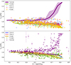 |
Fig. 5. Ionic electron temperature across all SFR–M⋆ and radial bins as a function of strong-line metallicity (P04). The two panels present identical temperature estimates. In the upper panel, OIII and SIII temperatures are binned in metallicity intervals of 0.05 dex; filled regions represent the 1σ percentile of distributions around the median values indicated by solid lines. The same binning procedure is applied to the low-ionization ionic temperatures in the lower panel. The error bars for OII, SII, and NII temperatures in the upper panel as well as OIII and SIII in the lower one correspond to the formal error obtained through the bootstrapping analysis, as detailed in Sect. 3.3. |
The behavior of the [OIII] temperature in Fig. 5 is noticeably divergent from that of the other temperatures. At low metallicities, the [OIII] temperatures are consistently higher than that of the low-ionization lines (by 600 K on average). At higher metallicity, however, the inferred [OIII] temperature increases to very high value, with an inflection point around 12 + log(O/H) = 8.5 as inferred from the P04 calibration. We considered this effect to be potentially associated with imperfections in the flux measurement in the presence of strong contamination at high metallicity, as discussed above. Alternatively, it could be associated with shocks or additional physical processes besides photoionization that may primarily affect the innermost, most highly ionized, section of the nebula Rickards Vaught et al. (2024). Whatever the origin of this behavior, its effect on the inferred [OIII] temperatures is significant enough to make us question their reliability. In this work we did not employ [OIII] temperatures in ionic abundance measurements, deeming them unreliable. A more accurate measurement of the [OIII] temperature requires either high spectral resolution observations, capable of identifying the sources of contamination in the high-metallicity regime, or a more accurate model for the physical source of the contamination emission.
3.4. T–T relations
The temperature of various ionization zones in HII regions is probed by different ions (e.g., Garnett 1992; Kennicutt et al. 2003). In this section we explore the relations between different electron temperatures (T–T relations) in 336 (56 × 6) bins. We adopted a bootstrapping analysis to mitigate the potential effects of the stacking process on our temperature determinations. In particular, for each radial bin in the SFR–M⋆ plane, we randomly selected 90% of the galaxies in the bin and generated 150 different bootstrapped stacks. We measured the line fluxes in each bootstrapped realization and used these fluxes to infer temperatures. Only realizations with temperature uncertainties below 200 K were considered reliable. Subsequently, the standard deviation obtained from the bootstrapped reliable temperatures served as the formal error estimate for each bin. Notably, these formal errors are several orders of magnitude larger than the actual temperature errors obtained from flux uncertainties.
As a result, we measured the electron temperatures encompassing a broad range of temperatures from ∼5000 K to approximately 12 000 K. In fitting the T–T relations we considered only temperatures with formal errors < 500 K and weight the data points by their uncertainties in both axes using inverse variance weighting. Additionally, we implemented a sigma clipping method (2σ) on the error-weighted temperatures to reduce the impact of outliers on the determination of the best fits.
For low-ionization ions ([OII], [NII], and [SII]) we see a strong correlation and fairly close to one-to-one relation between their respective temperatures (Fig. 6). The resulting best fits are consistent with linear relations with zero or small intercepts:
![Mathematical equation: $$ \begin{aligned} \mathrm T_{e}[NII]&= (0.97\pm 0.06) \times \mathrm T_{e}[OII] + (100\pm 600)\,\mathrm{K};\end{aligned} $$](/articles/aa/full_html/2025/01/aa51980-24/aa51980-24-eq2.gif) (2)
(2)
![Mathematical equation: $$ \begin{aligned} \mathrm T_{e}[SII]&= (1.03\pm 0.05)\times \mathrm T_{e}[OII] - (500\pm 500)\,\mathrm{K};\end{aligned} $$](/articles/aa/full_html/2025/01/aa51980-24/aa51980-24-eq3.gif) (3)
(3)
![Mathematical equation: $$ \begin{aligned} \mathrm T_{e}[SII]&= (1.04\pm 0.06)\times \mathrm T_{e}[NII] - (900\pm 600)\,\mathrm{K}. \end{aligned} $$](/articles/aa/full_html/2025/01/aa51980-24/aa51980-24-eq4.gif) (4)
(4)
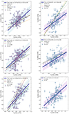 |
Fig. 6. Te data for [O II], [N II], [S II], and [S III] auroral lines for our galaxy sample in 56 SFR–M⋆ bins across six different radii. The columns are ordered by ionization zone relations: different low-ionized zones, Te, are compared in the left panels and low- and high-ionized zones, Te, are compared in the right. The solid lines indicate the linear fit to error-weighted sigma-clipped temperatures, and the dashed lines represent the one-to-one relation. The shaded regions (σ) represent the standard deviation of temperatures distributed around the fitted values. The number of data points (N°) is specified for each panel, and error bars represent the official temperature errors outlined in Sect. 3.4. The dashed-dotted green and red lines represent the T–T relations introduced by Zurita et al. (2021) and Méndez-Delgado et al. (2023; MD+23), respectively, while the dotted orange line shows the relation reported by Rogers et al. (2021). |
The quadruplet of auroral lines [O II]λλλλ7318, 7316,7329, 7330 is located in a region of the optical spectrum that suffers from extensive contamination from sky lines. The measurements of their flux may also be affected by phenomena including collisional de-excitation, imperfect reddening correction, and telluric emission from OH bands (e.g., Kennicutt et al. 2003; Pilyugin et al. 2006). These factors, in turn, introduce potential uncertainties the [OII] temperature, which has been considered in the literature as the least reliable among the low-ionization lines. In this work, however, we find excellent agreement between the low-ionization line temperatures, which models expect to be identical in a wide range of ionized gas conditions (e.g., Andrews & Martini 2013; Croxall et al. 2016)
The [SIII] ion probes the intermediate-ionization zone and its temperature is compared with that of the low-ionization ions in the right panels in Fig. 6. We find a moderate to strong positive correlation between Te[SIII] and the Te of low-ionization ions, with an average correlation coefficient of 0.53. We also observe a consistent deviation from the one-to-one relation, with [SIII] generally showing lower temperatures than [OII] and [SII]. The deviation between the [SIII] and low-ionization temperatures is larger at high temperatures (i.e., lower metallicities). Our findings indicate that Te[OII] exhibits a more rapid increase compared to Te, [SIII], align more closely with the empirical trend identified by Zurita et al. (2021), while, according to the predictions of the Vale Asari et al. (2016) photoionization models, the temperature Te[SIII] is expected to be slightly higher than Te[OII] by a consistent margin throughout the entire range of temperatures.
These relations have also been empirically established in previous investigations (e.g., Esteban et al. 2009; Pilyugin et al. 2009; Andrews & Martini 2013; Croxall et al. 2016; Zurita et al. 2021; Yates et al. 2020; Berg et al. 2020; Rogers et al. 2021; Rickards Vaught et al. 2024). The results presented in this section are generally in qualitative agreement with previous studies. Specifically, our findings align with those of Berg et al. (2020) and Zurita et al. (2021) for both low and high ionization zones, and with Rogers et al. (2021) and Méndez-Delgado et al. (2023) for low ionization zone temperatures. Additionally, the results of Rickards Vaught et al. (2024) are compatible with our findings regarding the comparison between [SIII] and low-ionization ionic temperatures.
3.5. Ionic abundances calculations
We calculated ionic abundances using PyNeb, using the electron temperature, electron density, and the appropriate flux ratio of the nebular emission line with respect to Hβ.
To calculate the abundance of O+ we used the [O II]λλ3726,3729 nebular lines and the error-weighted average temperature of low-ionized ions ([NII], [OII], and [SII]). This approach is supported by our finding in Sect. 3.4 that
![Mathematical equation: $$ \begin{aligned} T_{\rm [OII]} \approx T_{\rm [SII]} \approx T_{\rm [NII]}. \end{aligned} $$](/articles/aa/full_html/2025/01/aa51980-24/aa51980-24-eq5.gif) (5)
(5)
Furthermore, despite the high S/N of our stacked spectra, some stacks have OII or other low-ionization ion temperatures with errors exceeding the cutoff of 500 K. The averaging approach allows us to fold in these relatively weak detections by using alternative temperature measurements when one, especially OII, is excluded.
To estimate O++ abundances we used the [O III]4959,5007 Å fluxes and inferred the temperatures of [OIII] from that of the other ions applying the T–T relations from Rogers et al. (2021). In particular, we obtained our best estimate of the OIII temperature by using the median the temperatures obtained using the T–T relations from Rogers et al. (2021) relating T[OIII] with T[SIII],
![Mathematical equation: $$ \begin{aligned} T_{\rm [O III]} = 0.63 \times T_{\rm [S III]} + 3600, \end{aligned} $$](/articles/aa/full_html/2025/01/aa51980-24/aa51980-24-eq6.gif) (6)
(6)
and with the temperature of each of the measured low-ionization ions,
![Mathematical equation: $$ \begin{aligned} T_{\rm [O III]} = 1.30 \times T_{\rm low \ ion} - 2000. \end{aligned} $$](/articles/aa/full_html/2025/01/aa51980-24/aa51980-24-eq7.gif) (7)
(7)
We computed the ionic abundances of O+ and O++ ions for each stacked spectrum. Finally, we computed the total oxygen abundance as the sum of these two ionic abundances, neglecting higher ionization states. Moreover, through the use of MC simulations, we calculated the inferred oxygen abundance uncertainties by randomly perturbing all recorded line fluxes 1000 times, based on the assumption of a Gaussian noise distribution and their measured errors. We only considered temperatures with uncertainties below 500 K to categorize bins with well-detected auroral lines.
In Fig. 7, show the trends of O+ and O++ abundances (top panels) and their abundance ratios (bottom panel) with strong-line metallicity. As expected, O++/H+ ratio decreases with metallicity, while the O+/H+ ratio shows a positive slope in the whole metallicity range. The bottom panel of Fig. 3.5 demonstrates a decreasing O++ to O+ ratio with increasing metallicities. Incidentally, because of the lower O++ abundance at high metallicity, the overall oxygen abundance measurements are not very sensitive to the choice of T[OIII] in the high-metallicity regime.
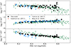 |
Fig. 7. O++ and O+ ionic abundances as a function of metallicity measured from the Pettini & Pagel (2004) O3N2 calibration. Our measurements of MaNGA data are compared to ionic abundances that are reproduced by employing the emission line fluxes reported in Guseva et al. (2011), Curti et al. (2017), and Berg et al. (2020). The ionic abundances, global and radially binned, are available online (see Tables B.5 and B.6). |
We compared these abundance trends with those obtained using data from the literature extracted from Guseva et al. (2011), Curti et al. (2017), and Berg et al. (2020). Guseva et al. (2011) used archival VLT/FORS1+UVES spectroscopic data to study a large sample of star-forming galaxies with low metallicity, encompassing a total of 121 spectra. The Curti et al. (2017) data consist of stacks of SDSS galaxies, while Berg et al. (2020) examined 190 individual HII regions in NGC 628, NGC 5194, NGC 5457, and NGC 3184, which were targeted by Multi-Object Double Spectrographs (MODS; Pogge et al. 2010) on the Large Binocular Telescope (LBT) as a part of the ongoing survey of the CHemical Abundances of Spirals (CHAOS; Berg et al. 2015). We used the emission line fluxes reported in these literature studies but recomputed chemical abundances following the same procedure adopted in this work. Our results are consistent with O+ and O++ abundances derived from those studies. Furthermore, we confirm that our findings remain consistent with these studies even when using the [OII] and [OIII] temperatures derived from their reported fluxes.
4. Results
4.1. Mass-metallicity relation
As shown in Fig. 8, we present the MZR obtained from our estimates of direct metallicity using SFR–M⋆ bins and stacking all the spectra in the 0.0–1.5 Re radial range. This leads to 54 measurements of metallicity as a function of M⋆ and SFR. The shaded areas represent the standard deviation of the entire sample (individual SFR–M⋆ bins) from the fit. For ease of visualization in Fig. 8, we divide the sample into mass bins of 0.1 dex width, with error bars representing the standard deviation of the metallicity distribution. In Fig. 8, we present a fit to metallicity values, adopting a slightly modified version of the Zahid et al. (2014) functional form, as introduced in Curti et al. (2020a), following the equation
 (8)
(8)
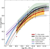 |
Fig. 8. MZR obtained using Te-based metallicities from the stacked spectra (solid brown line) compared to the MZR obtained using strong-line methods (P04 O3N2 and PG16) and relations from the literature. Direct-method measurements (8.5 < logM⋆/M⊙ < 11.0) are shown in brown, with the line representing the best fit following the Eq. (8) functional form, and the shaded region indicating the standard deviation of metallicity distributed around the fit. Metallicity measurements via empirical calibrations (PG16 and P04) from our sample are represented in gray and black, respectively. The comparisons with the characterizations of the MZR from Andrews & Martini (2013), Curti et al. (2020a), and Sanders et al. (2021) are depicted by the blue, purple, and green lines, respectively, along with their corresponding standard deviations. Metallicity values, global and radially binned, are available online (see Tables B.5 and B.6). |
Our best-fitting median MZR, determined using the direct method, asymptotes at 12 + log(O/H) = 8.73 ± 0.04, with a turnover at log(M⋆/M⊙) = 9.99 ± 0.18 and a low-mass-end slope of γ = 0.26 ± 0.07, as reported in Table 2. We also show the results of the same analysis on our sample using the P04 O3N2 and the PG16 (Pilyugin & Grebel 2016) strong-line metallicity calibration.
In previous studies, it has been shown that the shape of the local MZR exhibits notable differences depending on the metallicity indicator and calibration used (Kewley & Ellison 2008; López-Sánchez et al. 2012; Curti et al. 2020a). Therefore, the comparison of metallicities derived from different indicators and calibrations has the potential to introduce substantial biases. Nevertheless, our directly measured MZR, with a standard deviation of 0.08 dex, is both qualitatively and quantitatively consistent with the calibration values of P04 (0.07 dex standard deviation) within the associated uncertainties. The shape of the Te-MZR also agrees with PG16, albeit the absolute values provided by PG16 are consistently lower than other measurements, with metallicities barely reaching a maximum of 8.65. This behavior has been pointed out in previous studies, adopting a MaNGA sample (e.g., Duarte Puertas et al. 2022; Boardman et al. 2023).
Figure 8 also shows a comparison with characterizations of the MZR from the literature (Andrews & Martini 2013; Curti et al. 2020a; Sanders et al. 2021). Using stacked spectra from SDSS Andrews & Martini (2013) directly measure oxygen abundances for SFR–M⋆ bin. The MZR by Curti et al. (2020a) encompasses a mass range of 108 − 1011.5 M⊙ and is also based on the Te-derived metallicities from SDSS stacked spectra, albeit binned in the [OIII]λ5007/Hβ versus [OII]λ3727/Hβ plane. Lastly, Sanders et al. (2021) expanded upon the galaxy sample used by Andrews & Martini (2013), incorporating the sample of 38 dwarf galaxies from the Spitzer Local Volume Legacy survey (Berg et al. 2020) within a mass range of 108.5 − 1011.5 M⊙. They took into consideration the contributions from diffuse ionized gas (DIG) to the total emission line fluxes in integrated galaxy spectra, a factor they demonstrated leads to an overestimation of metallicity. This comparison shows that our directly measured metallicities using the MaNGA sample are qualitatively consistent with those from other studies, which employ different samples and various metallicity diagnostics.
4.2. Metallicity gradients
Figure 9 shows the Te-derived metallicity profiles out to 2.5 Re in 10 bins of M⋆ from ∼108.4 to ∼1011 M⊙. We note that, to reduce scatter and ensure smaller bin ranges at higher masses, Fig. 9 replaces the original mass bins from Fig. 2 with 0.25 dex bins, using the median mass of galaxies in each SFR − M⋆ bin. The dash-dotted lines show the median metallicity in each radial bin while the shaded regions show the standard deviation of data points of different SFR around the median. We can measure Te metallicity even in the farthest radial bin, 1.5–2.5 Re. However, to obtain more robust metallicity gradient slopes, we fit only radial bins up to 1.5 Re. This choice aligns with the common radius covered by MaNGA across the entire sample (see Sect. 2). Figure 9 shows the best fit linear relation between the oxygen abundance and the radius normalized to Re. In most cases the extrapolation of the linear fit agrees well with the measurements in the 1.5–2.5 Re radial bin.
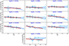 |
Fig. 9. Metallicity gradient of SFR–M⋆ bins with different stellar masses, separated by 0.25 dex. The solid lines represent a linear fit to SFR–M⋆ bins out to 1.5 Re. The dash-dotted line demonstrates the trend of the median metallicity of all bins up to 2.5 Re. The shaded region shows the standard deviation of metallicity distribution around the dash-dotted line. |
Figure 10 illustrates the correlation between the metallicity gradient and M⋆, MZGR. In this figure, we show the values derived from the linear fits (red) in Fig. 9 and the median slope of individual SFR–M⋆ bins within the specified mass range (green). We observe that, in both approaches, the slope of metallicity gradients exhibits variations across different stellar masses. It transitions from being relatively flat or slightly positive at log(M⋆/M⊙)≲9.2 to negative, reaching the most negative value around M⋆ ∼ 1010.3 M⊙. In bins with higher mass, there is a reversal of this trend, with gradients appearing shallower (see Table A.1). This observation is further validated by performing a third-order fit to the slopes of individual SFR–M⋆ bins, with the standard deviation of these slopes illustrated by the gray-shaded region.
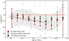 |
Fig. 10. Metallicity gradient across a radial span of 0.0–1.5 Re using the Te (red) and P04 calibration based on O3N2 (black) as a function of stellar mass. The red data points correspond to the slopes depicted in Fig. 9, with error bars indicating the uncertainty in the slope. Each SFR − M⋆ bin’s slopes are shown with gray points, while green points represent the median value of slopes within a specific mass range. The gray shaded area represents a third-degree polynomial fit to the slopes of all SFR-M bins. |
Similar qualitative characteristics in the shape of the metallicity profile are identified when utilizing the R231 metallicity calibrators of Maiolino et al. (2008) and Sanders et al. (2021).
5. Discussion
5.1. Metallicity gradient
The spatial resolution of MaNGA (1–2 kpc) can introduce a flattening of measured metallicity gradients due to resolution effects (Yuan et al. 2013; Carton et al. 2018; Acharyya et al. 2020). However, this resolution remains largely consistent across the sample, varying minimally with stellar mass except at the highest mass end (logM*/M⊙ > 10.5). Consequently, comparisons of metallicity gradients across different mass bins are expected to yield reliable differential measurements, with any resolution-induced bias affecting all but the most massive galaxies similarly.
Our findings are aligned with the Belfiore et al. (2017) study where they found nonlinear dependence of the metallicity gradient on stellar mass (109 − 1011 M⊙) with a smaller MaNGA (DR13) sample size and employing strong-line calibrations. Moreover, using SAMI Survey data, Poetrodjojo et al. (2018) corroborated the variations in the metallicity gradient with increasing stellar mass within a range of 109 − 1010.5 M⊙. Our results are also consistent with the findings of Mingozzi et al. (2020) using MaNGA data. They demonstrated a strong mass dependence of metallicity gradients, with galaxies in the mass range 10.2 ≲ log(M⋆/M⊙) ≲ 10.4 exhibiting the steepest negative gradients, employing various metallicity calibrations.
In this work, we aim to avoid oversimplifying the physical mechanisms underlying metallicity gradients and MZGR behavior, as a complete understanding requires both observational and theoretical perspectives. For instance, regarding the observed flattening of the metallicity gradient at the low-mass end, some studies attribute this effect to stellar feedback, which regulates metallicity before significant ISM and metal mixing occurs (e.g., Chisholm et al. 2018; Sharda et al. 2021). Alternatively, other studies suggest that gas mixing and wind recycling in the outer regions of galaxies may drive this flattening (e.g., Belfiore et al. 2017).
The region with the steepest gradient and highest curvature around 1010 − 10.5 M⊙ (shown in Fig. 10) could provide valuable insights into galaxy evolution and the key factors shaping galaxy characteristics from local to high redshift. For instance, Sharda et al. (2021) demonstrated that galaxies dominated by advection tend to flatten at the low-mass end, whereas accretion-dominated galaxies exhibit flattening at the high-mass end. Notably, they observed that advection and accretion do not simultaneously weaken, thereby ruling out diffusion as a primary gradient-smoothing mechanism. Their model indicates that the characteristic bend in the MZGR occurs when two major processes that influence gradient smoothing - accretion and inward gas advection - are at their lowest relative to metal production. Although the stellar mass at which this transition occurs may vary depending on model parameters and metallicity calibrations (see Poetrodjojo et al. 2021), their findings demonstrate that the presence of this bend is robust across different model assumptions.
At intermediate redshift, Carton et al. (2018) used MUSE (Multi Unit Spectroscopic Explorer) data and found marginal evidence of similar metallicity gradient trends (up to M⋆ ∼ 1010.5 M⊙) for a selection of 84 galaxies (0.1 < z < 0.8) employing a forward-modeling technique. At higher redshifts, Cheng et al. (2024) illustrated weak but significant anticorrelation between the metallicity gradient and the stellar mass in 238 star-forming galaxies at cosmic noon. Furthermore, Venturi et al. (2024) found flat gas-phase metallicity gradients in three systems at 6 < z < 8, and Vallini et al. (2024), reported a flat gradient at the epoch of reionization (z ∼ 7).
5.2. FMR(?)
The existence of a secondary dependence on SFR in the MZR remains a hotly debated topic in the literature. Several authors have confirmed the existence of the FMR (e.g., Mannucci et al. 2010; Andrews & Martini 2013; Hunt et al. 2016; Curti et al. 2020a, 2024; Pistis et al. 2024). Other studies question this conclusion by pointing out that, since most galaxies lie on a tight correlation between M⋆ and SFR, the FMR is driven by outliers and including and SFR dependence create a small or negligible reduction in the scatter of the MZR (Barrera-Ballesteros et al. 2017; Alvarez-Hurtado et al. 2022).
Moreover, most of these studies are based on subsamples of the same observational dataset, the SDSS spectroscopic survey. Despite the application of corrections (Brinchmann et al. 2004), the spectroscopic information is affected by aperture effects (e.g., Gomes et al. 2016; Iglesias-Páramo et al. 2016).
Moreover, in a recent study, Baker & Maiolino (2023) explored the dependence of gas metallicity on various galaxy parameters for 1000 star-forming galaxies from the MaNGA survey. Using different statistical methods such as the average dispersion, partial correlation coefficients, and random forest regression analysis, they suggest that part of the correlation between SFR and metallicity found in previous studies results from the correlation between gravitational potential and metallicity. Furthermore, recent investigations using IFS data have indicated that local processes, such as those involving gas metallicity, stellar mass surface density, and SFR density, may significantly influence global scaling relations (Barrera-Ballesteros et al. 2016; Sánchez-Menguiano et al. 2019; Baker et al. 2023).
Using the P04 O3N2 the existence of the FMR is clearly evident in Figs. 11 and 12, as metallicity decreases with increasing SFR across each mass bin. The existence and strength of the FMR depends, however, on the strong-line calibrator used. Using the calibration proposed by Dopita et al. (2016) we obtain a much weaker secondary trend with SFR (see Fig. 11). On average, the correlation coefficients between log(O/H) and SFR in fixed mass bins are −0.75 for P04 and −0.17 for the calibration of Dopita et al. (2016).
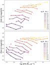 |
Fig. 11. Relationship between the global log(O/H) and the SFR for our sample color-coded for different stellar mass bins. In the upper panel, metallicities are calculated using the empirical calibration by Dopita et al. (2016), while in the lower panel, metallicities are determined via the calibration by Pettini & Pagel (2004). On average, the correlation coefficients between log(O/H) and SFR are −0.17 for the upper panel and −0.75 for the lower panel. |
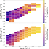 |
Fig. 12. SFR–M⋆ bins color-coded according to direct metallicity measurements (top panel) and P04 calibrations (bottom panel). Any missing bins are a result of either large temperature errors or a lower auroral line S/N that falls below the introduced cutoff (Sect. 3). |
In Fig. 12 we show each bin in the SFR–M⋆ plane color-coded by its metallicity from the Te method (top panel) and from the P04 O3N2 strong-line method (bottom panel). When employing the direct method (top panel) for measuring metallicity, this correlation largely disappears. In this case the average Pearson correlation coefficient between SFR and metallicity across the different mass bin is ρ ∼ −0.05. We tested these conclusion by modifying the bootstrapping procedure, stricter criteria for reliable fluxes and temperatures, using measured [OII] temperatures for determining its abundance, and employing both smaller and larger bins in SFR and M⋆ space. However, the results are robust to these modifications.
6. Summary and conclusion
In this study we have computed the Te metallicity across a radial span of 0.0–2.5 Re for 4140 star-forming galaxies, distributed across 56 SFR–M⋆ bins, using data from the MaNGA survey (DR17). The enhanced S/N achieved through the stacking procedure in SFR–M⋆ space enabled us to detect the auroral lines required to determine electron temperatures across various ionization zones, enabling the application of the Te method to measure direct metallicities. Our main results are summarized as follows:
-
We find excellent agreement between the low-ionization line temperatures traced by [OII], [SII], and [NII], with a nearly one-to-one relationship across a wide temperature range. [SIII], which traces the intermediate-ionization zone, generally has similar or lower temperatures compared to the low-ionization lines. The deviation between [SIII] and the low-ionization temperatures becomes more pronounced at higher temperatures, corresponding to lower metallicities.
-
The inferred [OIII] temperatures are in disagreement with the temperatures measured from other ions, especially at high metallicities. Such a deviation is particularly evident for 12 + log(O/H) > 8.5 as determined by the P04 calibration. We can potentially attribute this effect to potential imperfections in flux measurements due to significant spectral contamination at high metallicities. Such contamination of the [OIII]4363 line has previously been reported in the literature. While the precise nature of this contamination remains unclear, it is at least partially due to the presence of the [Fe II]λ4360 line. However, the higher [OIII] temperatures are obtained even after fitting the [Fe II]λ4360 flux and explicitly constraining it to 0.73 times that of the nearby isolated [Fe II]λ4288. A physical origin for the higher T[OIII] temperature (e.g., additional heating in the high-ionization zone) cannot be ruled out. In this work we considered the [OIII] temperatures unreliable and excluded them from ionic abundance measurements.
-
We calculated ionic abundances of O+ using the low-ionization temperatures and O++ based on the other measured electron temperatures. The relative abundance of O++ to O+ decreases with metallicity, indicating a reduced impact of O++ or the estimate of T[OIII] on final oxygen abundance estimations at higher metallicities.
-
We derived the MZR from direct metallicity estimates using SFR-M⋆ bins and stacking spectra in the 0.0 − 1.5 Re radial range, which resulted in 56 metallicity measurements. The measured MZR is in good agreement with literature values.
-
We calculated the Te metallicity gradient across the radial range 0.0–1.5 Re for 4140 star-forming galaxies distributed among 56 SFR–M⋆ bins. The metallicity gradients reveal a linear relation between oxygen abundances at different radii normalized to Re for stellar masses from approximately 108.4 to 1011 M⊙. We demonstrate the correlation between metallicity gradient slopes and stellar mass, with slopes transitioning from flat or slightly positive at low stellar masses to negative around 1010.3 M⊙, and then becoming shallower at higher masses. This pattern is in agreement with previous studies based on smaller MaNGA and SAMI Survey samples in the local Universe and with MUSE data at higher redshifts. We used different metallicity calibrators, including R23 and strong-line methods, but our findings remained consistent.
-
We investigated the presence of the FMR. We show that strong-line methods can be used to recover the FMR, although the strength of the FMR signal depends on the strong-line calibrator used. However, using the direct method to measure metallicity reveals no clear FMR.
Further spatially resolved investigations may contribute to a better understanding of the FMR and its existence on local scales. Building on this work, stacking spaxels and deriving a relation between the gas-phase metallicity, stellar mass surface density, and SFR surface density could address open questions regarding the global versus local effects of the FMR, irrespective of the parent galaxy properties.
Data availability
Full catalogs from this work (i.e., Tables B.1–B.6) are available at the CDS via anonymous ftp to cdsarc.cds.unistra.fr (130.79.128.5) or via https://cdsarc.cds.unistra.fr/viz-bin/cat/J/A+A/693/A150
R23 = ([O II]λ3726,28+[O III]λ4959,5007)/Hβ.
Acknowledgments
AK thanks Amirnezam Amiri, Sirio Belli, Noah Rogers, Erin Kado-Fong, and Mirko Curti for the constructive and insightful discussions that significantly contributed to the development of this work. FB acknowledges funding from the INAF Fundamental Astrophysics program 2022. Funding for the Sloan Digital Sky Survey IV has been provided by the Alfred P. Sloan Foundation, the U.S. Department of Energy Office of Science, and the Participating Institutions. SDSS-IV acknowledges support and resources from the Center for High Performance Computing at the University of Utah. SDSS-IV is managed by the Astrophysical Research Consortium for the Participating Institutions, listed on the SDSS website www.sdss4.org.
References
- Abdurro’uf, Accetta, K., Aerts, C., et al. 2022, ApJS, 259, 35 [NASA ADS] [CrossRef] [Google Scholar]
- Acharyya, A., Krumholz, M. R., Federrath, C., et al. 2020, MNRAS, 495, 3819 [NASA ADS] [CrossRef] [Google Scholar]
- Alvarez-Hurtado, P., Barrera-Ballesteros, J. K., Sánchez, S. F., et al. 2022, ApJ, 929, 47 [NASA ADS] [CrossRef] [Google Scholar]
- Andrews, B. H., & Martini, P. 2013, ApJ, 765, 140 [NASA ADS] [CrossRef] [Google Scholar]
- Baker, W. M., & Maiolino, R. 2023, MNRAS, 521, 4173 [CrossRef] [Google Scholar]
- Baker, W. M., Maiolino, R., Belfiore, F., et al. 2023, MNRAS, 519, 1149 [Google Scholar]
- Baldwin, J. A., Phillips, M. M., & Terlevich, R. 1981, PASP, 93, 5 [Google Scholar]
- Barrera-Ballesteros, J. K., Heckman, T. M., Zhu, G. B., et al. 2016, MNRAS, 463, 2513 [NASA ADS] [CrossRef] [Google Scholar]
- Barrera-Ballesteros, J. K., Sánchez, S. F., Heckman, T., Blanc, G. A., & MaNGA Team 2017, ApJ, 844, 80 [CrossRef] [Google Scholar]
- Belfiore, F., Maiolino, R., Maraston, C., et al. 2016, MNRAS, 461, 3111 [Google Scholar]
- Belfiore, F., Maiolino, R., Tremonti, C., et al. 2017, MNRAS, 469, 151 [Google Scholar]
- Belfiore, F., Maiolino, R., Bundy, K., et al. 2018, MNRAS, 477, 3014 [Google Scholar]
- Belfiore, F., Westfall, K. B., Schaefer, A., et al. 2019, AJ, 158, 160 [CrossRef] [Google Scholar]
- Berg, D. A., Skillman, E. D., Croxall, K. V., et al. 2015, ApJ, 806, 16 [NASA ADS] [CrossRef] [Google Scholar]
- Berg, D. A., Pogge, R. W., Skillman, E. D., et al. 2020, ApJ, 893, 96 [NASA ADS] [CrossRef] [Google Scholar]
- Blanton, M. R., Kazin, E., Muna, D., Weaver, B. A., & Price-Whelan, A. 2011, AJ, 142, 31 [NASA ADS] [CrossRef] [Google Scholar]
- Boardman, N., Wild, V., Heckman, T., et al. 2023, MNRAS, 520, 4301 [NASA ADS] [CrossRef] [Google Scholar]
- Boissier, S., & Prantzos, N. 1999, MNRAS, 307, 857 [NASA ADS] [CrossRef] [Google Scholar]
- Bothwell, M. S., Maiolino, R., Kennicutt, R., et al. 2013, MNRAS, 433, 1425 [Google Scholar]
- Brinchmann, J., Charlot, S., White, S. D. M., et al. 2004, MNRAS, 351, 1151 [Google Scholar]
- Bryant, J. J., Owers, M. S., Robotham, A. S. G., et al. 2015, MNRAS, 447, 2857 [Google Scholar]
- Cappellari, M. 2017, MNRAS, 466, 798 [Google Scholar]
- Cappellari, M., & Copin, Y. 2003, MNRAS, 342, 345 [Google Scholar]
- Cappellari, M., & Emsellem, E. 2004, PASP, 116, 138 [Google Scholar]
- Carton, D., Brinchmann, J., Contini, T., et al. 2018, MNRAS, 478, 4293 [NASA ADS] [CrossRef] [Google Scholar]
- Chabrier, G. 2003, PASP, 115, 763 [Google Scholar]
- Cheng, Y., Giavalisco, M., Simons, R. C., et al. 2024, ApJ, 964, 94 [NASA ADS] [CrossRef] [Google Scholar]
- Chiappini, C., Matteucci, F., & Romano, D. 2001, ApJ, 554, 1044 [NASA ADS] [CrossRef] [Google Scholar]
- Chisholm, J., Tremonti, C., & Leitherer, C. 2018, MNRAS, 481, 1690 [NASA ADS] [CrossRef] [Google Scholar]
- Croom, S. M., Lawrence, J. S., Bland-Hawthorn, J., et al. 2012, MNRAS, 421, 872 [NASA ADS] [Google Scholar]
- Croxall, K. V., Pogge, R. W., Berg, D. A., Skillman, E. D., & Moustakas, J. 2016, ApJ, 830, 4 [NASA ADS] [CrossRef] [Google Scholar]
- Curti, M., Cresci, G., Mannucci, F., et al. 2017, MNRAS, 465, 1384 [Google Scholar]
- Curti, M., Mannucci, F., Cresci, G., & Maiolino, R. 2020a, MNRAS, 491, 944 [Google Scholar]
- Curti, M., Maiolino, R., Cirasuolo, M., et al. 2020b, MNRAS, 492, 821 [CrossRef] [Google Scholar]
- Curti, M., Maiolino, R., Curtis-Lake, E., et al. 2024, A&A, 684, A75 [NASA ADS] [CrossRef] [EDP Sciences] [Google Scholar]
- Dopita, M. A., Kewley, L. J., Sutherland, R. S., & Nicholls, D. C. 2016, Ap&SS, 361, 61 [NASA ADS] [CrossRef] [Google Scholar]
- Duarte Puertas, S., Vilchez, J. M., Iglesias-Páramo, J., et al. 2022, A&A, 666, A186 [NASA ADS] [CrossRef] [EDP Sciences] [Google Scholar]
- Ellison, S. L., Patton, D. R., Simard, L., & McConnachie, A. W. 2008, AJ, 135, 1877 [NASA ADS] [CrossRef] [Google Scholar]
- Esteban, C., Bresolin, F., Peimbert, M., et al. 2009, ApJ, 700, 654 [NASA ADS] [CrossRef] [Google Scholar]
- Garnett, D. R. 1992, AJ, 103, 1330 [NASA ADS] [CrossRef] [Google Scholar]
- Giovanelli, R., Haynes, M. P., Salzer, J. J., et al. 1994, AJ, 107, 2036 [NASA ADS] [CrossRef] [Google Scholar]
- Gomes, J. M., Papaderos, P., Vílchez, J. M., et al. 2016, A&A, 586, A22 [NASA ADS] [CrossRef] [EDP Sciences] [Google Scholar]
- Guseva, N. G., Izotov, Y. I., Stasińska, G., et al. 2011, A&A, 529, A149 [NASA ADS] [CrossRef] [EDP Sciences] [Google Scholar]
- Hao, C.-N., Kennicutt, R. C., Johnson, B. D., et al. 2011, ApJ, 741, 124 [Google Scholar]
- Hemler, Z. S., Torrey, P., Qi, J., et al. 2021, MNRAS, 506, 3024 [NASA ADS] [CrossRef] [Google Scholar]
- Henriques, B. M. B., Yates, R. M., Fu, J., et al. 2020, MNRAS, 491, 5795 [NASA ADS] [CrossRef] [Google Scholar]
- Ho, I. T., Kudritzki, R.-P., Kewley, L. J., et al. 2015, MNRAS, 448, 2030 [NASA ADS] [CrossRef] [Google Scholar]
- Hunt, L., Dayal, P., Magrini, L., & Ferrara, A. 2016, MNRAS, 463, 2002 [NASA ADS] [CrossRef] [Google Scholar]
- Iglesias-Páramo, J., Vílchez, J. M., Rosales-Ortega, F. F., et al. 2016, ApJ, 826, 71 [Google Scholar]
- Izotov, Y. I., Stasińska, G., Meynet, G., Guseva, N. G., & Thuan, T. X. 2006, A&A, 448, 955 [CrossRef] [EDP Sciences] [Google Scholar]
- Jones, T., Sanders, R., Roberts-Borsani, G., et al. 2020, ApJ, 903, 150 [CrossRef] [Google Scholar]
- Ju, M., Wang, X., Jones, T., et al. 2024, arXiv e-prints [arXiv:2409.01616] [Google Scholar]
- Kauffmann, G., Heckman, T. M., Tremonti, C., et al. 2003, MNRAS, 346, 1055 [Google Scholar]
- Kennicutt, R. C., Jr., Bresolin, F., & Garnett, D. R. 2003, ApJ, 591, 801 [NASA ADS] [CrossRef] [Google Scholar]
- Kewley, L. J., & Ellison, S. L. 2008, ApJ, 681, 1183 [Google Scholar]
- Kewley, L. J., Dopita, M. A., Sutherland, R. S., Heisler, C. A., & Trevena, J. 2001, ApJ, 556, 121 [Google Scholar]
- Larson, R. B. 1976, MNRAS, 176, 31 [NASA ADS] [CrossRef] [Google Scholar]
- Law, D. R., Yan, R., Bershady, M. A., et al. 2015, AJ, 150, 19 [CrossRef] [Google Scholar]
- Law, D. R., Cherinka, B., Yan, R., et al. 2016, AJ, 152, 83 [Google Scholar]
- Law, D. R., Westfall, K. B., Bershady, M. A., et al. 2021, AJ, 161, 52 [NASA ADS] [CrossRef] [Google Scholar]
- Li, Z., Wang, X., Cai, Z., et al. 2022, ApJ, 929, L8 [NASA ADS] [CrossRef] [Google Scholar]
- López-Sánchez, R., Dopita, M. A., Kewley, L. J., et al. 2012, MNRAS, 426, 2630 [CrossRef] [Google Scholar]
- Luridiana, V., Morisset, C., & Shaw, R. A. 2012, IAU Symp., 283, 422 [NASA ADS] [Google Scholar]
- Luridiana, V., Morisset, C., & Shaw, R. A. 2015, A&A, 573, A42 [NASA ADS] [CrossRef] [EDP Sciences] [Google Scholar]
- Ma, X., Hopkins, P. F., Feldmann, R., et al. 2017, MNRAS, 466, 4780 [Google Scholar]
- Maiolino, R., & Mannucci, F. 2019, A&ARv, 27, 3 [Google Scholar]
- Maiolino, R., Nagao, T., Grazian, A., et al. 2008, A&A, 488, 463 [NASA ADS] [CrossRef] [EDP Sciences] [Google Scholar]
- Mannucci, F., Cresci, G., Maiolino, R., Marconi, A., & Gnerucci, A. 2010, MNRAS, 408, 2115 [NASA ADS] [CrossRef] [Google Scholar]
- Maraston, C., Hill, L., Thomas, D., et al. 2020, MNRAS, 496, 2962 [Google Scholar]
- Matteucci, F., & Francois, P. 1989, MNRAS, 239, 885 [Google Scholar]
- Méndez-Delgado, J. E., Esteban, C., García-Rojas, J., et al. 2023, MNRAS, 523, 2952 [CrossRef] [Google Scholar]
- Mingozzi, M., Belfiore, F., Cresci, G., et al. 2020, A&A, 636, A42 [NASA ADS] [CrossRef] [EDP Sciences] [Google Scholar]
- Mott, A., Spitoni, E., & Matteucci, F. 2013, MNRAS, 435, 2918 [Google Scholar]
- Nakajima, K., & Ouchi, M. 2014, MNRAS, 442, 900 [Google Scholar]
- Nakajima, K., Ouchi, M., Isobe, Y., et al. 2023, arXiv e-prints [arXiv:2301.12825] [Google Scholar]
- O’Donnell, J. E. 1994, ApJ, 422, 158 [Google Scholar]
- Osterbrock, D. E. 1989, Astrophysics of Gaseous Nebulae and Active Galactic Nuclei (University Science Books) [Google Scholar]
- Pagel, B. E. J. 1997, Nucleosynthesis and Chemical Evolution of Galaxies (Cambridge, UK: Cambridge University Press) [Google Scholar]
- Pagel, B. E. J., Simonson, E. A., Terlevich, R. J., & Edmunds, M. G. 1992, MNRAS, 255, 325 [CrossRef] [Google Scholar]
- Pettini, M., & Pagel, B. E. J. 2004, MNRAS, 348, L59 [NASA ADS] [CrossRef] [Google Scholar]
- Pezzulli, G., & Fraternali, F. 2016, MNRAS, 455, 2308 [Google Scholar]
- Pietrinferni, A., Cassisi, S., Salaris, M., & Castelli, F. 2004, ApJ, 612, 168 [Google Scholar]
- Pilkington, K., Few, C. G., Gibson, B. K., et al. 2012, A&A, 540, A56 [NASA ADS] [CrossRef] [EDP Sciences] [Google Scholar]
- Pilyugin, L. S., & Grebel, E. K. 2016, MNRAS, 457, 3678 [NASA ADS] [CrossRef] [Google Scholar]
- Pilyugin, L. S., Vílchez, J. M., & Thuan, T. X. 2006, MNRAS, 370, 1928 [NASA ADS] [CrossRef] [Google Scholar]
- Pilyugin, L. S., Mattsson, L., Vílchez, J. M., & Cedrés, B. 2009, MNRAS, 398, 485 [NASA ADS] [CrossRef] [Google Scholar]
- Pilyugin, L. S., Grebel, E. K., & Zinchenko, I. A. 2015, MNRAS, 450, 3254 [CrossRef] [Google Scholar]
- Pistis, F., Pollo, A., Figueira, M., et al. 2024, A&A, 683, A203 [NASA ADS] [CrossRef] [EDP Sciences] [Google Scholar]
- Poetrodjojo, H., Groves, B., Kewley, L. J., et al. 2018, MNRAS, 479, 5235 [Google Scholar]
- Poetrodjojo, H., Groves, B., Kewley, L. J., et al. 2021, MNRAS, 502, 3357 [NASA ADS] [CrossRef] [Google Scholar]
- Pogge, R. W., Atwood, B., Brewer, D. F., et al. 2010, SPIE Conf. Ser., 7735, 77350A [Google Scholar]
- Prantzos, N., & Boissier, S. 2000, MNRAS, 313, 338 [NASA ADS] [CrossRef] [Google Scholar]
- Rafelski, M., Wolfe, A. M., Prochaska, J. X., Neeleman, M., & Mendez, A. J. 2012, ApJ, 755, 89 [NASA ADS] [CrossRef] [Google Scholar]
- Rickards Vaught, R. J., Sandstrom, K. M., Belfiore, F., et al. 2024, ApJ, 966, 130 [NASA ADS] [CrossRef] [Google Scholar]
- Rogers, N. S. J., Skillman, E. D., Pogge, R. W., et al. 2021, ApJ, 915, 21 [NASA ADS] [CrossRef] [Google Scholar]
- Rosales-Ortega, F. F., Díaz, A. I., Kennicutt, R. C., & Sánchez, S. F. 2011, MNRAS, 415, 2439 [NASA ADS] [CrossRef] [Google Scholar]
- Sánchez, S. F., Rosales-Ortega, F. F., Iglesias-Páramo, J., et al. 2014, A&A, 563, A49 [CrossRef] [EDP Sciences] [Google Scholar]
- Sánchez-Blázquez, P., Peletier, R. F., Jiménez-Vicente, J., et al. 2006, MNRAS, 371, 703 [Google Scholar]
- Sánchez-Menguiano, L., Sánchez, S. F., Pérez, I., et al. 2016, A&A, 587, A70 [NASA ADS] [CrossRef] [EDP Sciences] [Google Scholar]
- Sánchez-Menguiano, L., Sánchez Almeida, J., Muñoz-Tuñón, C., et al. 2019, ApJ, 882, 9 [CrossRef] [Google Scholar]
- Sanders, R. L., Shapley, A. E., Kriek, M., et al. 2015, ApJ, 799, 138 [NASA ADS] [CrossRef] [Google Scholar]
- Sanders, R. L., Shapley, A. E., Jones, T., et al. 2021, ApJ, 914, 19 [CrossRef] [Google Scholar]
- Sharda, P., Krumholz, M. R., Wisnioski, E., et al. 2021, MNRAS, 502, 5935 [NASA ADS] [CrossRef] [Google Scholar]
- Simons, R. C., Papovich, C., Momcheva, I., et al. 2021, ApJ, 923, 203 [NASA ADS] [CrossRef] [Google Scholar]
- Smee, S. A., Gunn, J. E., Uomoto, A., et al. 2013, AJ, 146, 32 [Google Scholar]
- Spolaor, M., Kobayashi, C., Forbes, D. A., Couch, W. J., & Hau, G. K. T. 2010, MNRAS, 408, 272 [Google Scholar]
- Tinsley, B. M. 1980, Fund. Cosmic Phys., 5, 287 [Google Scholar]
- Tremonti, C. A., Heckman, T. M., Kauffmann, G., et al. 2004, ApJ, 613, 898 [Google Scholar]
- Vale Asari, N., Stasińska, G., Morisset, C., & Cid Fernandes, R. 2016, MNRAS, 460, 1739 [NASA ADS] [CrossRef] [Google Scholar]
- Vallini, L., Witstok, J., Sommovigo, L., et al. 2024, MNRAS, 527, 10 [Google Scholar]
- Vazdekis, A., Koleva, M., Ricciardelli, E., Röck, B., & Falcón-Barroso, J. 2016, MNRAS, 463, 3409 [Google Scholar]
- Venturi, G., Carniani, S., Parlanti, E., et al. 2024, A&A, 691, A19 [NASA ADS] [CrossRef] [EDP Sciences] [Google Scholar]
- Wake, D. A., Bundy, K., Diamond-Stanic, A. M., et al. 2017, AJ, 154, 86 [Google Scholar]
- Wang, X., Jones, T. A., Treu, T., et al. 2020, ApJ, 900, 183 [NASA ADS] [CrossRef] [Google Scholar]
- Wang, X., Jones, T., Vulcani, B., et al. 2022, ApJ, 938, L16 [NASA ADS] [CrossRef] [Google Scholar]
- Westfall, K. B., Cappellari, M., Bershady, M. A., et al. 2019, AJ, 158, 231 [Google Scholar]
- Yan, R., Tremonti, C., Bershady, M. A., et al. 2016, AJ, 151, 8 [Google Scholar]
- Yan, R., Chen, Y., Lazarz, D., et al. 2019, ApJ, 883, 175 [Google Scholar]
- Yates, R. M., Schady, P., Chen, T. W., Schweyer, T., & Wiseman, P. 2020, A&A, 634, A107 [NASA ADS] [CrossRef] [EDP Sciences] [Google Scholar]
- Yuan, T. T., Kewley, L. J., & Rich, J. 2013, ApJ, 767, 106 [NASA ADS] [CrossRef] [Google Scholar]
- Zahid, H. J., Kashino, D., Silverman, J. D., et al. 2014, ApJ, 792, 75 [NASA ADS] [CrossRef] [Google Scholar]
- Zinchenko, I. A., Pilyugin, L. S., Grebel, E. K., Sánchez, S. F., & Vílchez, J. M. 2016, MNRAS, 462, 2715 [Google Scholar]
- Zurita, A., Florido, E., Bresolin, F., Pérez-Montero, E., & Pérez, I. 2021, MNRAS, 500, 2359 [Google Scholar]
Appendix A: Metallicity gradient slopes table
Appendix B: Online catalogs
Radially binned integrated spectra (extract).
Global integrated spectra (extract).
Radially binned emission line fluxes and their uncertainties (extract). The structure and description of the table columns are laid out here, with the complete version available at the CDS.
Global emission line fluxes and their uncertainties in SFRM⋆ bins (extract). The structure and description of the table columns are laid out here, with the complete version available at the CDS.
Radially binned inferred physical parameters, electron temperature, ionic abundance, Te and stron-line metallicity for all the bins (extract). The structure and description of the table columns are laid out here, with the complete version available at the CDS.
Global inferred physical parameters, including electron temperature, ionic abundances, Te-based metallicity, and strong-line metallicity for all bins (extract). The structure and description of the table columns are laid out here, with the complete version available at the CDS.
All Tables
Radially binned emission line fluxes and their uncertainties (extract). The structure and description of the table columns are laid out here, with the complete version available at the CDS.
Global emission line fluxes and their uncertainties in SFRM⋆ bins (extract). The structure and description of the table columns are laid out here, with the complete version available at the CDS.
Radially binned inferred physical parameters, electron temperature, ionic abundance, Te and stron-line metallicity for all the bins (extract). The structure and description of the table columns are laid out here, with the complete version available at the CDS.
Global inferred physical parameters, including electron temperature, ionic abundances, Te-based metallicity, and strong-line metallicity for all bins (extract). The structure and description of the table columns are laid out here, with the complete version available at the CDS.
All Figures
|
Fig. 1. Redshift–M⋆ plane of the MaNGA sample utilized in this study. The star-forming galaxies (see Sect. 2.1) chosen for the study of gas-phase metallicity are shown in green and the entire MaNGA DR17 sample in gray. The redshift and stellar mass distributions for the selected and full samples used in this work are shown as green and gray histograms. |
| In the text | |
|
Fig. 2. Position of the bins used for spectral stacking in this work in the SFR–M⋆ plane. Each rectangle represents a bin, color-coded according to its median strong-line metallicity using the Pettini & Pagel (2004) calibration and extinction-corrected emission lines from the MaNGA DAP catalog. The number of galaxies in each bin is reported. In the inset in the lower right, our stacking grid is shown superimposed on the distribution of individual MaNGA star-forming galaxies in the SFR–M⋆ plane. The integrated spectra, global and radially binned, are available online (see Tables B.2 and B.1). |
| In the text | |
|
Fig. 3. Topmost panel: Stacked spectrum of a SFR–M⋆ bin (M⋆ = 108.65 M⊙ and SFR = 1−1.3 M⊙ yr−1), showing zoomed-in views of the spectral fits around some of the strong nebular lines. In the subplots below we zoom in on the fit residuals in specific spectral regions to highlight the detection of faint, temperature-sensitive auroral lines (in red) and other nearby emission lines (blue). The dashed green lines represent the standard deviation of residual fits in each wavelength window. The emission line fluxes and associated uncertainties, global and radially binned, are available online (see Tables B.3 and B.4). |
| In the text | |
|
Fig. 4. Spectral residuals in the wavelength range near the [O III]λ4363 line, after stellar continuum subtraction. The red and blue Gaussian fits represent [O III]λ4363 and [Fe II]λ4360 emission lines, respectively. The dashed lines illustrate the standard deviation of residual fits in the corresponding windows. The strong-line metallicity and measured [O III] temperature of each stack are reported in the panels. The contamination of the [O III]λ4363 line becomes more relevant with increasing metallicity. |
| In the text | |
|
Fig. 5. Ionic electron temperature across all SFR–M⋆ and radial bins as a function of strong-line metallicity (P04). The two panels present identical temperature estimates. In the upper panel, OIII and SIII temperatures are binned in metallicity intervals of 0.05 dex; filled regions represent the 1σ percentile of distributions around the median values indicated by solid lines. The same binning procedure is applied to the low-ionization ionic temperatures in the lower panel. The error bars for OII, SII, and NII temperatures in the upper panel as well as OIII and SIII in the lower one correspond to the formal error obtained through the bootstrapping analysis, as detailed in Sect. 3.3. |
| In the text | |
|
Fig. 6. Te data for [O II], [N II], [S II], and [S III] auroral lines for our galaxy sample in 56 SFR–M⋆ bins across six different radii. The columns are ordered by ionization zone relations: different low-ionized zones, Te, are compared in the left panels and low- and high-ionized zones, Te, are compared in the right. The solid lines indicate the linear fit to error-weighted sigma-clipped temperatures, and the dashed lines represent the one-to-one relation. The shaded regions (σ) represent the standard deviation of temperatures distributed around the fitted values. The number of data points (N°) is specified for each panel, and error bars represent the official temperature errors outlined in Sect. 3.4. The dashed-dotted green and red lines represent the T–T relations introduced by Zurita et al. (2021) and Méndez-Delgado et al. (2023; MD+23), respectively, while the dotted orange line shows the relation reported by Rogers et al. (2021). |
| In the text | |
|
Fig. 7. O++ and O+ ionic abundances as a function of metallicity measured from the Pettini & Pagel (2004) O3N2 calibration. Our measurements of MaNGA data are compared to ionic abundances that are reproduced by employing the emission line fluxes reported in Guseva et al. (2011), Curti et al. (2017), and Berg et al. (2020). The ionic abundances, global and radially binned, are available online (see Tables B.5 and B.6). |
| In the text | |
|
Fig. 8. MZR obtained using Te-based metallicities from the stacked spectra (solid brown line) compared to the MZR obtained using strong-line methods (P04 O3N2 and PG16) and relations from the literature. Direct-method measurements (8.5 < logM⋆/M⊙ < 11.0) are shown in brown, with the line representing the best fit following the Eq. (8) functional form, and the shaded region indicating the standard deviation of metallicity distributed around the fit. Metallicity measurements via empirical calibrations (PG16 and P04) from our sample are represented in gray and black, respectively. The comparisons with the characterizations of the MZR from Andrews & Martini (2013), Curti et al. (2020a), and Sanders et al. (2021) are depicted by the blue, purple, and green lines, respectively, along with their corresponding standard deviations. Metallicity values, global and radially binned, are available online (see Tables B.5 and B.6). |
| In the text | |
|
Fig. 9. Metallicity gradient of SFR–M⋆ bins with different stellar masses, separated by 0.25 dex. The solid lines represent a linear fit to SFR–M⋆ bins out to 1.5 Re. The dash-dotted line demonstrates the trend of the median metallicity of all bins up to 2.5 Re. The shaded region shows the standard deviation of metallicity distribution around the dash-dotted line. |
| In the text | |
|
Fig. 10. Metallicity gradient across a radial span of 0.0–1.5 Re using the Te (red) and P04 calibration based on O3N2 (black) as a function of stellar mass. The red data points correspond to the slopes depicted in Fig. 9, with error bars indicating the uncertainty in the slope. Each SFR − M⋆ bin’s slopes are shown with gray points, while green points represent the median value of slopes within a specific mass range. The gray shaded area represents a third-degree polynomial fit to the slopes of all SFR-M bins. |
| In the text | |
|
Fig. 11. Relationship between the global log(O/H) and the SFR for our sample color-coded for different stellar mass bins. In the upper panel, metallicities are calculated using the empirical calibration by Dopita et al. (2016), while in the lower panel, metallicities are determined via the calibration by Pettini & Pagel (2004). On average, the correlation coefficients between log(O/H) and SFR are −0.17 for the upper panel and −0.75 for the lower panel. |
| In the text | |
|
Fig. 12. SFR–M⋆ bins color-coded according to direct metallicity measurements (top panel) and P04 calibrations (bottom panel). Any missing bins are a result of either large temperature errors or a lower auroral line S/N that falls below the introduced cutoff (Sect. 3). |
| In the text | |
Current usage metrics show cumulative count of Article Views (full-text article views including HTML views, PDF and ePub downloads, according to the available data) and Abstracts Views on Vision4Press platform.
Data correspond to usage on the plateform after 2015. The current usage metrics is available 48-96 hours after online publication and is updated daily on week days.
Initial download of the metrics may take a while.