| Issue |
A&A
Volume 693, January 2025
|
|
|---|---|---|
| Article Number | A265 | |
| Number of page(s) | 27 | |
| Section | Extragalactic astronomy | |
| DOI | https://doi.org/10.1051/0004-6361/202451296 | |
| Published online | 22 January 2025 | |
The persistent shadow of the supermassive black hole of M87
II. Model comparisons and theoretical interpretations
1
Massachusetts Institute of Technology Haystack Observatory, 99 Millstone Road, Westford, MA, 01886, USA
2
National Astronomical Observatory of Japan, 2-21-1 Osawa, Mitaka, Tokyo, 181-8588, Japan
3
Black Hole Initiative at Harvard University, 20 Garden Street, Cambridge, MA, 02138, USA
4
Departament d’Astronomia i Astrofísica, Universitat de València, C. Dr. Moliner 50, E-46100 Burjassot, València, Spain
5
Instituto de Astrofísica de Andalucía-CSIC, Glorieta de la Astronomía s/n, E-18008 Granada, Spain
6
Max-Planck-Institut für Radioastronomie, Auf dem Hügel 69, D-53121 Bonn, Germany
7
Department of Physics, Faculty of Science, Universiti Malaya, 50603 Kuala Lumpur, Malaysia
8
Department of Physics & Astronomy, The University of Texas at San Antonio, One UTSA Circle, San Antonio, TX, 78249, USA
9
Physics & Astronomy Department, Rice University, Houston, TX, 77005-1827, USA
10
Center for Astrophysics | Harvard & Smithsonian, 60 Garden Street, Cambridge, MA, 02138, USA
11
Institute of Astronomy and Astrophysics, Academia Sinica, 11F of Astronomy-Mathematics Building, AS/NTU No. 1, Sec. 4, Roosevelt Rd., Taipei, 106216, Taiwan, ROC
12
Observatori Astronòmic, Universitat de València, C. Catedrático José Beltrán 2, E-46980 Paterna, València, Spain
13
Department of Space, Earth and Environment, Chalmers University of Technology, Onsala Space Observatory, SE-43992 Onsala, Sweden
14
Steward Observatory and Department of Astronomy, University of Arizona, 933 N. Cherry Ave., Tucson, AZ, 85721, USA
15
Yale Center for Astronomy & Astrophysics, Yale University, 52 Hillhouse Avenue, New Haven, CT, 06511, USA
16
Astronomy Department, Universidad de Concepción, Casilla 160-C, Concepción, Chile
17
Department of Physics, University of Illinois, 1110 West Green Street, Urbana, IL, 61801, USA
18
Fermi National Accelerator Laboratory, MS209, P.O. Box 500 Batavia, IL, 60510, USA
19
Department of Astronomy and Astrophysics, University of Chicago, 5640 South Ellis Avenue, Chicago, IL, 60637, USA
20
East Asian Observatory, 660 N. A’ohoku Place, Hilo, HI, 96720, USA
21
James Clerk Maxwell Telescope (JCMT), 660 N. A’ohoku Place, Hilo, HI, 96720, USA
22
California Institute of Technology, 1200 East California Boulevard, Pasadena, CA, 91125, USA
23
Institute of Astronomy and Astrophysics, Academia Sinica, 645 N. A’ohoku Place, Hilo, HI, 96720, USA
24
Department of Physics and Astronomy, University of Hawaii at Manoa, 2505 Correa Road, Honolulu, HI, 96822, USA
25
Institut de Radioastronomie Millimétrique (IRAM), 300 rue de la Piscine, F-38406 Saint Martin d’Hères, France
26
Perimeter Institute for Theoretical Physics, 31 Caroline Street North, Waterloo, ON, N2L 2Y5, Canada
27
Department of Physics and Astronomy, University of Waterloo, 200 University Avenue West, Waterloo, ON, N2L 3G1, Canada
28
Waterloo Centre for Astrophysics, University of Waterloo, Waterloo, ON, N2L 3G1, Canada
29
Department of Astrophysics, Institute for Mathematics, Astrophysics and Particle Physics (IMAPP), Radboud University, P.O. Box 9010 6500 GL Nijmegen, The Netherlands
30
Department of Astronomy, University of Massachusetts, Amherst, MA, 01003, USA
31
Kavli Institute for Cosmological Physics, University of Chicago, 5640 South Ellis Avenue, Chicago, IL, 60637, USA
32
Department of Physics, University of Chicago, 5720 South Ellis Avenue, Chicago, IL, 60637, USA
33
Enrico Fermi Institute, University of Chicago, 5640 South Ellis Avenue, Chicago, IL, 60637, USA
34
Princeton Gravity Initiative, Jadwin Hall, Princeton University, Princeton, NJ, 08544, USA
35
Data Science Institute, University of Arizona, 1230 N. Cherry Ave., Tucson, AZ, 85721, USA
36
Program in Applied Mathematics, University of Arizona, 617 N. Santa Rita, Tucson, AZ, 85721, USA
37
Cornell Center for Astrophysics and Planetary Science, Cornell University, Ithaca, NY, 14853, USA
38
Shanghai Astronomical Observatory, Chinese Academy of Sciences, 80 Nandan Road, Shanghai, 200030, PR China
39
Key Laboratory of Radio Astronomy and Technology, Chinese Academy of Sciences, A20 Datun Road, Chaoyang District, Beijing, 100101, PR China
40
Korea Astronomy and Space Science Institute, Daedeok-daero 776, Yuseong-gu, Daejeon, 34055, Republic of Korea
41
Department of Astronomy, Yonsei University, Yonsei-ro 50, Seodaemun-gu, 03722 Seoul, Republic of Korea
42
Physics Department, Fairfield University, 1073 North Benson Road, Fairfield, CT, 06824, USA
43
Department of Astronomy, University of Illinois at Urbana-Champaign, 1002 West Green Street, Urbana, IL, 61801, USA
44
Instituto de Astronomía, Universidad Nacional Autónoma de México (UNAM), Apdo Postal 70-264 Ciudad de México, Mexico
45
Institut für Theoretische Physik, Goethe-Universität Frankfurt, Max-von-Laue-Straße 1, D-60438 Frankfurt am Main, Germany
46
Research Center for Astronomical Computing, Zhejiang Laboratory, Hangzhou, 311100, People’s Republic of China
47
Tsung-Dao Lee Institute, Shanghai Jiao Tong University, Shengrong Road 520, Shanghai, 201210, People’s Republic of China
48
Department of Astrophysical Sciences, Peyton Hall, Princeton University, Princeton, NJ, 08544, USA
49
Dipartimento di Fisica “E. Pancini”, Università di Napoli “Federico II”, Compl. Univ. di Monte S. Angelo, Edificio G, Via Cinthia, I-80126 Napoli, Italy
50
INFN Sez. di Napoli, Compl. Univ. di Monte S. Angelo, Edificio G, Via Cinthia, I-80126 Napoli, Italy
51
Wits Centre for Astrophysics, University of the Witwatersrand, 1 Jan Smuts Avenue, Braamfontein, Johannesburg, 2050, South Africa
52
Department of Physics, University of Pretoria, Hatfield, Pretoria, 0028, South Africa
53
Centre for Radio Astronomy Techniques and Technologies, Department of Physics and Electronics, Rhodes University, Makhanda, 6140, South Africa
54
ASTRON, Oude Hoogeveensedijk 4, 7991 PD Dwingeloo, The Netherlands
55
LESIA, Observatoire de Paris, Université PSL, CNRS, Sorbonne Université, Université de Paris, 5 place Jules Janssen, F-92195 Meudon, France
56
JILA and Department of Astrophysical and Planetary Sciences, University of Colorado, Boulder, CO, 80309, USA
57
National Astronomical Observatories, Chinese Academy of Sciences, 20A Datun Road, Chaoyang District, Beijing, 100101, PR China
58
Las Cumbres Observatory, 6740 Cortona Drive, Suite 102, Goleta, CA, 93117-5575, USA
59
Department of Physics, University of California, Santa Barbara, CA, 93106-9530, USA
60
National Radio Astronomy Observatory, 520 Edgemont Road, Charlottesville, VA, 22903, USA
61
Department of Electrical Engineering and Computer Science, Massachusetts Institute of Technology, 32-D476, 77 Massachusetts Ave., Cambridge, MA, 02142, USA
62
Google Research, 355 Main St., Cambridge, MA, 02142, USA
63
Institut für Theoretische Physik und Astrophysik, Universität Würzburg, Emil-Fischer-Str. 31, D-97074 Würzburg, Germany
64
Department of History of Science, Harvard University, Cambridge, MA, 02138, USA
65
Department of Physics, Harvard University, Cambridge, MA, 02138, USA
66
NCSA, University of Illinois, 1205 W. Clark St., Urbana, IL, 61801, USA
67
Instituto de Astronomia, Geofísica e Ciências Atmosféricas, Universidade de São Paulo, R. do Matão, 1226, São Paulo, SP, 05508-090, Brazil
68
Dipartimento di Fisica, Università degli Studi di Cagliari, SP Monserrato-Sestu km 0.7, I-09042 Monserrato (CA), Italy
69
INAF - Osservatorio Astronomico di Cagliari, via della Scienza 5, I-09047 Selargius (CA), Italy
70
INFN, sezione di Cagliari, I-09042 Monserrato (CA), Italy
71
Institute for Mathematics and Interdisciplinary Center for Scientific Computing, Heidelberg University, Im Neuenheimer Feld 205, Heidelberg, 69120, Germany
72
Institut für Theoretische Physik, Universität Heidelberg, Philosophenweg 16, 69120 Heidelberg, Germany
73
CP3-Origins, University of Southern Denmark, Campusvej 55, DK-5230 Odense, Denmark
74
Instituto Nacional de Astrofísica, Óptica y Electrónica, Apartado Postal 51 y 216, 72000 Puebla Pue., Mexico
75
Consejo Nacional de Humanidades, Ciencia y Tecnología, Av. Insurgentes Sur 1582, 03940 Ciudad de México, Mexico
76
Key Laboratory for Research in Galaxies and Cosmology, Chinese Academy of Sciences, Shanghai, 200030, PR China
77
Graduate School of Science, Nagoya City University, Yamanohata 1, Mizuho-cho, Mizuho-ku, Nagoya, 467-8501 Aichi, Japan
78
Mizusawa VLBI Observatory, National Astronomical Observatory of Japan, 2-12 Hoshigaoka, Mizusawa, Oshu, Iwate, 023-0861, Japan
79
Department of Physics, McGill University, 3600 rue University, Montréal, QC, H3A 2T8, Canada
80
Trottier Space Institute at McGill, 3550 rue University, Montréal, QC, H3A 2A7, Canada
81
NOVA Sub-mm Instrumentation Group, Kapteyn Astronomical Institute, University of Groningen, Landleven 12, 9747 AD Groningen, The Netherlands
82
Department of Astronomy, School of Physics, Peking University, Beijing, 100871, PR China
83
Kavli Institute for Astronomy and Astrophysics, Peking University, Beijing, 100871, PR China
84
Department of Astronomical Science, The Graduate University for Advanced Studies (SOKENDAI), 2-21-1 Osawa, Mitaka, Tokyo, 181-8588, Japan
85
Department of Astronomy, Graduate School of Science, The University of Tokyo, 7-3-1 Hongo, Bunkyo-ku, Tokyo, 113-0033, Japan
86
The Institute of Statistical Mathematics, 10-3 Midori-cho, Tachikawa, Tokyo, 190-8562, Japan
87
Department of Statistical Science, The Graduate University for Advanced Studies (SOKENDAI), 10-3 Midori-cho, Tachikawa, Tokyo, 190-8562, Japan
88
Kavli Institute for the Physics and Mathematics of the Universe, The University of Tokyo, 5-1-5 Kashiwanoha, Kashiwa, 277-8583, Japan
89
Leiden Observatory, Leiden University, Postbus 2300, 9513 RA Leiden, The Netherlands
90
ASTRAVEO LLC, PO Box 1668 Gloucester, MA, 01931, USA
91
Applied Materials Inc., 35 Dory Road, Gloucester, MA, 01930, USA
92
Institute for Astrophysical Research, Boston University, 725 Commonwealth Ave., Boston, MA, 02215, USA
93
University of Science and Technology, Gajeong-ro 217, Yuseong-gu, Daejeon, 34113, Republic of Korea
94
Institute for Cosmic Ray Research, The University of Tokyo, 5-1-5 Kashiwanoha, Kashiwa, Chiba, 277-8582, Japan
95
Joint Institute for VLBI ERIC (JIVE), Oude Hoogeveensedijk 4, 7991 PD Dwingeloo, The Netherlands
96
Department of Physics, Ulsan National Institute of Science and Technology (UNIST), Ulsan, 44919, Republic of Korea
97
Department of Physics, Korea Advanced Institute of Science and Technology (KAIST), 291 Daehak-ro, Yuseong-gu, Daejeon, 34141, Republic of Korea
98
Kogakuin University of Technology & Engineering, Academic Support Center, 2665-1 Nakano, Hachioji, Tokyo, 192-0015, Japan
99
Graduate School of Science and Technology, Niigata University, 8050 Ikarashi 2-no-cho, Nishi-ku, Niigata, 950-2181, Japan
100
Physics Department, National Sun Yat-Sen University, No. 70, Lien-Hai Road, Kaosiung City, 80424, Taiwan, ROC
101
School of Astronomy and Space Science, Nanjing University, Nanjing, 210023, PR China
102
Key Laboratory of Modern Astronomy and Astrophysics, Nanjing University, Nanjing, 210023, PR China
103
INAF-Istituto di Radioastronomia, Via P. Gobetti 101, I-40129 Bologna, Italy
104
Common Crawl Foundation, 9663 Santa Monica Blvd. 425, Beverly Hills, CA, 90210, USA
105
Instituto de Física, Pontificia Universidad Católica de Valparaíso, Casilla, 4059 Valparaíso, Chile
106
INAF-Istituto di Radioastronomia & Italian ALMA Regional Centre, Via P. Gobetti 101, I-40129 Bologna, Italy
107
Department of Physics, National Taiwan University, No. 1, Sec. 4, Roosevelt Rd., Taipei, 106216, Taiwan, ROC
108
Instituto de Radioastronomía y Astrofísica, Universidad Nacional Autónoma de México, Morelia, 58089, Mexico
109
David Rockefeller Center for Latin American Studies, Harvard University, 1730 Cambridge Street, Cambridge, MA, 02138, USA
110
Yunnan Observatories, Chinese Academy of Sciences, 650011 Kunming, Yunnan Province, PR China
111
Center for Astronomical Mega-Science, Chinese Academy of Sciences, 20A Datun Road, Chaoyang District, Beijing, 100012, PR China
112
Key Laboratory for the Structure and Evolution of Celestial Objects, Chinese Academy of Sciences, 650011 Kunming, PR China
113
Anton Pannekoek Institute for Astronomy, University of Amsterdam, Science Park 904, 1098 XH Amsterdam, The Netherlands
114
Gravitation and Astroparticle Physics Amsterdam (GRAPPA) Institute, University of Amsterdam, Science Park 904, 1098 XH Amsterdam, The Netherlands
115
School of Physics and Astronomy, Shanghai Jiao Tong University, 800 Dongchuan Road, Shanghai, 200240, PR China
116
Institut de Radioastronomie Millimétrique (IRAM), Avenida Divina Pastora 7, Local 20, E-18012 Granada, Spain
117
National Institute of Technology, Hachinohe College, 16-1 Uwanotai, Tamonoki, Hachinohe City, Aomori, 039-1192, Japan
118
Research Center for Astronomy, Academy of Athens, Soranou Efessiou 4, 115 27 Athens, Greece
119
Department of Physics, Villanova University, 800 Lancaster Avenue, Villanova, PA, 19085, USA
120
Physics Department, Washington University, CB 1105, St. Louis, MO, 63130, USA
121
Departamento de Matemática da Universidade de Aveiro and Centre for Research and Development in Mathematics and Applications (CIDMA), Campus de Santiago, 3810-193 Aveiro, Portugal
122
School of Physics, Georgia Institute of Technology, 837 State St NW, Atlanta, GA, 30332, USA
123
School of Space Research, Kyung Hee University, 1732, Deogyeong-daero, Giheung-gu, Yongin-si, Gyeonggi-do, 17104, Republic of Korea
124
Canadian Institute for Theoretical Astrophysics, University of Toronto, 60 St. George Street, Toronto, ON, M5S 3H8, Canada
125
Dunlap Institute for Astronomy and Astrophysics, University of Toronto, 50 St. George Street, Toronto, ON, M5S 3H4, Canada
126
Canadian Institute for Advanced Research, 180 Dundas St West, Toronto, ON, M5G 1Z8, Canada
127
Dipartimento di Fisica, Università di Trieste, I-34127 Trieste, Italy
128
INFN Sez. di Trieste, I-34127 Trieste, Italy
129
Department of Physics, National Taiwan Normal University, No. 88, Sec. 4, Tingzhou Rd., Taipei 116, Taiwan, ROC
130
Center of Astronomy and Gravitation, National Taiwan Normal University, No. 88, Sec. 4, Tingzhou Road, Taipei, 116, Taiwan, ROC
131
Finnish Centre for Astronomy with ESO, University of Turku, FI-20014 Turun Yliopisto, Finland
132
Aalto University Metsähovi Radio Observatory, Metsähovintie 114, FI-02540 Kylmälä, Finland
133
Gemini Observatory/NSF NOIRLab, 670 N. A’ohōkū Place, Hilo, HI, 96720, USA
134
Frankfurt Institute for Advanced Studies, Ruth-Moufang-Strasse 1, D-60438 Frankfurt, Germany
135
School of Mathematics, Trinity College, Dublin 2, Ireland
136
Department of Physics, University of Toronto, 60 St. George Street, Toronto, ON, M5S 1A7, Canada
137
Department of Physics, Tokyo Institute of Technology, 2-12-1 Ookayama, Meguro-ku, Tokyo, 152-8551, Japan
138
Hiroshima Astrophysical Science Center, Hiroshima University, 1-3-1 Kagamiyama, Higashi-Hiroshima, Hiroshima, 739-8526, Japan
139
Aalto University Department of Electronics and Nanoengineering, PL 15500, FI-00076 Aalto, Finland
140
Jeremiah Horrocks Institute, University of Central Lancashire, Preston, PR1 2HE, UK
141
National Biomedical Imaging Center, Peking University, Beijing, 100871, PR China
142
College of Future Technology, Peking University, Beijing, 100871, PR China
143
Tokyo Electron Technology Solutions Limited, 52 Matsunagane, Iwayado, Esashi, Oshu, Iwate, 023-1101, Japan
144
Department of Physics and Astronomy, University of Lethbridge, Lethbridge, Alberta, T1K 3M4, Canada
145
Netherlands Organisation for Scientific Research (NWO), Postbus 93138, 2509 AC Den Haag, The Netherlands
146
Frontier Research Institute for Interdisciplinary Sciences, Tohoku University, Sendai, 980-8578, Japan
147
Astronomical Institute, Tohoku University, Sendai, 980-8578, Japan
148
Department of Physics and Astronomy, Seoul National University, Gwanak-gu, Seoul, 08826, Republic of Korea
149
University of New Mexico, Department of Physics and Astronomy, Albuquerque, NM, 87131, USA
150
Physics Department, Brandeis University, 415 South Street, Waltham, MA, 02453, USA
151
Tuorla Observatory, Department of Physics and Astronomy, University of Turku, FI-20014 Turun Yliopisto, Finland
152
Radboud Excellence Fellow of Radboud University, Nijmegen, The Netherlands
153
School of Natural Sciences, Institute for Advanced Study, 1 Einstein Drive, Princeton, NJ, 08540, USA
154
School of Physics, Huazhong University of Science and Technology, Wuhan, Hubei, 430074, PR China
155
Mullard Space Science Laboratory, University College London, Holmbury St. Mary, Dorking, Surrey, RH5 6NT, UK
156
Center for Astronomy and Astrophysics and Department of Physics, Fudan University, Shanghai, 200438, PR China
157
Astronomy Department, University of Science and Technology of China, Hefei, 230026, PR China
158
Department of Physics and Astronomy, Michigan State University, 567 Wilson Rd, East Lansing, MI, 48824, USA
⋆⋆⋆ Corresponding author; This email address is being protected from spambots. You need JavaScript enabled to view it.
Received:
28
June
2024
Accepted:
8
October
2024
Abstract
The Event Horizon Telescope (EHT) observation of M87∗ in 2018 has revealed a ring with a diameter that is consistent with the 2017 observation. The brightest part of the ring is shifted to the southwest from the southeast. In this paper, we provide theoretical interpretations for the multi-epoch EHT observations for M87∗ by comparing a new general relativistic magnetohydrodynamics model image library with the EHT observations for M87∗ in both 2017 and 2018. The model images include aligned and tilted accretion with parameterized thermal and nonthermal synchrotron emission properties. The 2018 observation again shows that the spin vector of the M87∗ supermassive black hole is pointed away from Earth. A shift of the brightest part of the ring during the multi-epoch observations can naturally be explained by the turbulent nature of black hole accretion, which is supported by the fact that the more turbulent retrograde models can explain the multi-epoch observations better than the prograde models. The EHT data are inconsistent with the tilted models in our model image library. Assuming that the black hole spin axis and its large-scale jet direction are roughly aligned, we expect the brightest part of the ring to be most commonly observed 90 deg clockwise from the forward jet. This prediction can be statistically tested through future observations.
Key words: accretion, accretion disks / black hole physics / gravitation / galaxies: active / galaxies: individual: M87 / galaxies: jets
NASA Hubble Fellowship Program, Einstein Fellow.
Yushan Fellow program, Yushan young fellow.
© The Authors 2025
 Open Access article, published by EDP Sciences, under the terms of the Creative Commons Attribution License (https://creativecommons.org/licenses/by/4.0), which permits unrestricted use, distribution, and reproduction in any medium, provided the original work is properly cited.
This article is published in open access under the Subscribe to Open model. This email address is being protected from spambots. You need JavaScript enabled to view it. to support open access publication.
1. Introduction
The first images by the Event Horizon Telescope (EHT) of the supermassive black hole (SMBH) in the heart of the M87 galaxy (M87∗) revealed a ring structure with a diameter of approximately five times the projected Schwarzschild radius of a 6.5 × 10⁹ M⊙ black hole (M87* 2017 I; M87* 2017 II; M87* 2017 III; M87* 2017 IV; M87* 2017 V; M87* 2017 VI). The EHT Collaboration recently published two new images of the M87∗ ring based on EHT data that were collected in April 2018 (M87* 2018 I, hereafter Paper I), almost exactly one year after the first observations. While the persistent ring structure revealed in the new images strongly supports the idea that the central depression of the M87∗ image is indeed the shadow of an event horizon of a supermassive object (e.g., Hilbert 1917; Bardeen 2018; Luminet 1979; Jaroszynski & Kurpiewski 1997; Falcke et al. 2000, M87* 2017 VI, Wielgus et al. 2020), the new data show a different brightness distribution in the ring. The new observations therefore place additional constraints on physical models of the emitting plasma close to the event horizon.
The conventional model for M87∗ is a black hole surrounded by a magnetized, geometrically thick, optically thin, radiatively inefficient, advection dominated, rotating accretion disk (e.g., Ichimaru 1977; Rees et al. 1982; Narayan & Yi 1994, 1995; Reynolds et al. 1996) that launches a relativistic jet. There is no consensus model for the jet-launching mechanism, but the two main scenarios are that the jet is either dominated by Poynting flux and extracts rotational energy from the supermassive black hole (Blandford & Znajek 1977) and/or that the jet is a magnetohydrodynamically collimated wind from the accretion disk that is launched close to the event horizon (Blandford & Payne 1982; Lynden-Bell 2006). The jet from M87∗ is clearly visible at longer radio wavelengths, in optical light, X-rays, and even γ-rays as an elongated feature that is resolved from submilliarcsecond to arcsecond scales (EHT MWL Science Working Group 2021; Lu et al. 2023).
The synchrotron emission from the disk-jet system close to the black hole is gravitationally lensed and Doppler boosted so that it appears to an external observer as an asymmetric ring structure. Because of astrophysical uncertainties and strong gravity, the physical interpretation of the ring emission is not straightforward and typically involves forward modeling using either semianalytic models (Broderick & Loeb 2009) or numerical simulations (e.g., Dexter et al. 2012; Mościbrodzka et al. 2016; Fromm et al. 2022).
The theoretical interpretations of the first 2017 EHT images of M87∗ have been presented in three preceding works (M87* 2017 V, M87* 2017 VIII, M87* 2017 IX). In M87* 2017 V, we created a library of 60 000 mock black hole images based on general relativistic magnetohydrodynamic (GRMHD) simulations of black hole accretion. The library surveyed different black hole spins and electron temperature parameterizations, and two distinct accretion flow modes: the standard and normal evolution (SANE) models, and the magnetically arrested disk (MAD) models. The initial setup for all the simulations featured a magnetized torus of plasma orbiting in the equatorial plane of the black hole. The different types of magnetic field geometry in the initial torus evolve to either the SANE or the MAD state. In M87* 2017 V, we constrained the models using M87 EHT 2017 data, observational jet power, and the M87 core X-ray luminosity. The models that passed these observational constraints included both SANEs and MADs, both with positive and negative spins. The sign of the spin is positive here when the accretion flow angular momentum and black hole spin are parallel, and it is negative when they are antiparallel (a counter-rotating, or retrograde, accretion flow). M87* 2017 V reported two main findings. First, the southern brightness asymmetry in the image strongly supports the interpretation that the spin axis of the M87 black hole points away from Earth. Second, it was predicted that if the black hole spin axis is normal to the disk (parallel to the large-scale jet axis), then future observations would most often show the brightest part of the ring appearing counterclockwise from the position seen in the 2017 observations.
Polarimetric images are more sensitive than total intensity alone to the plasma properties around the supermassive black hole. In a subsequent publication (M87* 2017 VIII), we compared the library of GRMHD simulations (72 000 images in total, extending the previous library with additional models for electron thermodynamics) to the 2017 linear polarimetric image of the M87∗ ring (M87* 2017 VII). We found that models that fell within the allowed ranges of the measured polarimetric characteristics are typically MAD. The observed, azimuthally dominated electric vector position angle (EVPA) pattern is usually inconsistent with SANE simulations. Although several SANE snapshots are consistent with EHT polarimetric observations, these models fail to produce sufficient jet power. The M87* 2017 VIII constraints narrowed the range of allowed mass accretion rates onto the M87 black hole horizon, Ṁ, to (3 − 20)×10−4 M⊙/yr. The near horizon jet power, Pjet, was narrowed down to 1042 − 1043 ergs s−1. The measurements of circular polarization on horizon scales of M87* presented in M87* 2017 IX did not change these conclusions.
The current paper is the second in a series of papers dedicated to the analysis of the EHT 2018 observations. In this paper, we focus on the theoretical interpretation of the observed total intensity of M87∗. To do this, we prepared an updated image library that covers a wider range of possible synchrotron emission natures and parameters of the surrounding plasma, and our images are based on more advanced GRMHD simulations. Considering the constraints imposed by multi-epoch observations, we compare the model images separately with both the 2018 (Paper I) and the initial (2017) observations of M87∗. The information derived from these comparisons is then combined to constrain the GRMHD models and draw new conclusions about the physical conditions around the supermassive black hole and to constrain the properties of the supermassive black hole itself, assuming that the 2017 and 2018 observations represent a typical state of the source.
The paper is structured as follows. In Sect. 2 we provide a list of the new observational constraints to motivate the more advanced library of GRMHD simulations. In Sect. 3 we describe our library. In Sect. 4 we describe our data-model comparison scheme and present the results of these comparisons. We discuss the new results in Sect. 5 and conclude in Sect. 6.
2. New observational constraints and expectations
Figure 1 (top and bottom left panels) shows representative reconstructed images of M87∗ based on the 2017 and 2018 datasets. The 2018 image reconstructions of M87∗ show the bright ring of emission with a diameter1 as; this angular size is consistent with the 2017 EHT measurements (
 as, M87* 2017 VI) and also with measurements from the less precise 2009-2013 proto-EHT data (Wielgus et al. 2020), but with a significantly different position angle of the brightest part of the ring (rotation by ∼30° from ∼180° as measured in 2017 to ∼210° in the 2018 data).
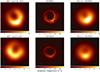 |
Fig. 1. Representative reconstructed images and model images of M87∗. Left panels: EHT images of M87∗ from the 2018 (M87* 2018 I; Paper I of this series) and 2017 (M87* 2017 IV) campaigns. Middle panels: Example GRMHD model images drawn from the same model at two different times. Right panels: Theoretical images convolved with a 20 μas FWHM Gaussian beam. |
The shift in the observed brightness position angle is expected from both observational precedent and theoretical predictions. Observationally, an analysis of historical VLBI data at 230 GHz using a prototype EHT array indicates even more variability on the horizon scale between 2009 and 2017 (Wielgus et al. 2020). Theoretically, images from GRMHD simulations feature significant variability in their image features. The middle and right panel in Fig. 1 show two snapshots from an example movie based on the same GRMHD simulation and their corresponding image when convolved with a beam similar to EHT resolutions. These frames illustrate that the observed shift in the brightest location on the ring can naturally arise from the turbulent nature of the accretion environment around a black hole. The 2018 images of M87∗ are consistent with the forecasts we made in M87* 2017 V. Compared to the 2017 images, the 2018 observed ring brightness distribution is closer to the mean value expected from coaxial models in which the black hole spin axis is aligned with the orientation of the large-scale jet seen at lower radio frequencies (Walker et al. 2018).
Additional constraints come from the coordinated simultaneous broadband multiwavelength observations of M87 carried out during the EHT campaigns in April 2017 and 2018 by the EHT Multiwavelength (MWL) Science Working Group (EHT MWL Science Working Group 2024). These observations covered more than 17 decades in frequency from radio (cm wavelength) to very high-energy (VHE) γ-rays (> 100 GeV). In April 2017, the source was found to be in a historically low state at all frequencies (EHT MWL Science Working Group 2021), but in April 2018, M87 underwent a γ-ray flaring episode (EHT MWL Science Working Group 2024), the first detected episode since 2010, with the peak on April 21 (MJD 58229.07). The VHE γ-ray flux doubled within a period of 36 hours, which enabled us to constrain the size of the VHE γ-ray emitting region to  , where δ is the standard Doppler beaming factor (Aharonian et al. 2006). This timescale is consistent with the γ-ray variability arising from the EHT-emitting region, or from a larger region in a more relativistic part of the jet. While the radio and millimeter (mm) core fluxes are compatible with (or potentially lower than) the April 2017 emission, a likely longer-term core flux enhancement was also observed in the X-ray band.
For neither the 2017 nor the 2018 observation can heuristic single-zone models fit the entire SED, suggesting the need for a stratified model. More sophisticated modeling will be needed to localize the γ-ray flare, and nonthermal processes will need to be included. Intriguingly, the hint of a decline in the submm core flux observed in 2018 is a prediction of reconnection-powered VHE flare mechanisms near the event horizon, which may lead to mass ejections out of the EHT-resolved region (Ripperda et al. 2022; Gelles et al. 2022; Hakobyan et al. 2023; Jia et al. 2023). This dip was not a statistically significant detection in 2018, but the possibility argues for more coordinated MWL observations, particularly between EHT and VHE facilities, to determine the location of the flare events.
In this work, we extend the previously constructed GRMHD libraries that were used to interpret M87 EHT observations. The new models are motivated by (1) a more limited set of the old models, which were not in steady state and did not include radiation and tilt, and (2) lower-frequency (86 GHz) observations by Cui et al. (2023), which motivate the exploration of tilted models that may lead to jet precession. The theoretical models are compared to selected EHT observations. Selected best-bet models, according to EHT constraints and jet power constraints, are discussed in the context of the radio and high-energy constraints.
3. Image library of the extended GRMHD simulations
Our numerical model library consists of a number of 3D GRMHD simulations of gas from a magnetized torus accreting onto a black hole and producing a jet. Table 1 summarizes all GRMHD models used in this work, together with details of their parameters. The parameters that are common across different simulation codes include the dimensionless black hole spin (a*), the adiabatic index in the adiabatic equation of state (Γad), the final time of the simulation (tf), the outer radius of the computational domain (rout), and the numerical resolution of the simulation in three dimensions (3D). Compared to the previous image library (M87* 2017 V), most of the images in our new library were computed based on GRMHD simulations evolved for a longer time (> 25 × 103GM/c3 ≈ 25 years), with model images derived from an interval at the end of the simulation with a length of 5 × 10³GM/c3 ≈ 5 yr.
GRMHD simulation library.
The black hole spin is described by the dimensionless spin parameter a* ≡ Jc/GM2 (e.g., Koide et al. 2000; De Villiers et al. 2003; Gammie et al. 2003; Porth et al. 2019), where J, M, G, and c are the black hole spin angular momentum, black hole mass, gravitational constant, and speed of light, respectively. The black hole spin is a free parameter within
 (1)
(1)
We assumed unless stated otherwise that the angular momentum of the accretion flow, the spin of the black hole, and the large-scale jet are coaxial. The inclination is defined as the angle between the accretion flow angular momentum and the line of sight, so that i = 0° implies that the accretion flow angular momentum is pointed at the observer. Positive (negative) spin implies that the angular momentum of the accretion flow and the black hole spin are aligned (anti-aligned), and thus, that the accretion flow is prograde (retrograde). When the angle between the approaching jet and the line of sight is 17° (e.g., Walker et al. 2018) then the model inclination can be either 17° or 163°.
M87* 2017 V showed that in coaxial models, the ring asymmetry follows the spin. In models in which the spin is pointed along the approaching jet (toward Earth), the mean position of the peak brightness on the ring is 90° counterclockwise from the jet, at a position angle of 20°. In models in which the spin is pointed away from Earth (along the counterjet), the mean position of the peak brightness on the ring is about 90° clockwise from the jet, at a position angle of 200°. Physically, this arises from a combination of effects (Doppler beaming, lensing, and aberration) that are difficult to separate in a relativistic context, but which all affect the fluid-frame frequency at which synchrotron emission is produced. Because GRMHD models are turbulent, the position of the peak brightness fluctuates around these expected values. M87* 2017 V concluded that because the peak brightness on the ring in the 2017 data was closer to a PA = 200° than 20°, the spin direction was pointed away from Earth.
All GRMHD simulations in this work began with a hydrodynamic torus of gas (Fishbone & Moncrief 1976) with a constant adiabatic index Γad seeded with a loop of poloidal magnetic fields, except for the radiative model. For the radiative GRMHD simulation, the initial torus followed Penna et al. (2013), and a variable adiabatic index (Sądowski et al. 2017) was used. These initial conditions for the simulations were reported in the papers related to the simulations (Prather 2022; Chatterjee & Narayan 2022; Cruz-Osorio et al. 2022; Fromm et al. 2022; Chatterjee et al. 2020; Chael et al. 2019a).
The accreting gas eventually becomes highly turbulent due to disk instabilities such as the magneto-rotational instability (MRI; Balbus & Hawley 1991), and occasionally, the magnetized Rayleigh–Taylor instabilities (e.g., Ripperda et al. 2022). The initial magnetic flux content of the disk determines the evolution of the accretion flow and therefore sets the magnetic flux at the black hole event horizon ϕBH. The horizon magnetic flux is an important quantity in our simulations as it determines the expected jet power according to the Blandford & Znajek (1977) effect.
As in M87* 2017 V, we considered two different accretion states depending on the mean magnetic flux crossing one hemisphere of the event horizon, ϕBH: (i) a weakly magnetized accretion flow (“SANE”; ϕBH ≈ 1; Narayan et al. 2012; Porth et al. 2019), and (ii) a magnetically arrested disk (“MAD”; ϕBH ≈ 15; Bisnovatyi-Kogan & Ruzmaikin 1974; Igumenshchev et al. 2003; Narayan et al. 2003). ϕBH is defined2 as the dimensionless form of the absolute magnetic flux (ΦBH) threading a hemisphere at the horizon, that is,  .
.
SANE accretion flows show MRI-driven disk turbulence and produce relativistic jets with powers Pjet ≲ 0.1 Ṁc2. MADs are characterized by dynamically strong magnetic fields near the black hole. MADs occasionally exhibit eruptions of magnetic flux tubes that affect the disk evolution (Chatterjee & Narayan 2022). MADs also show highly efficient jets with powers that can exceed the available accretion power for high black hole spins, Pjet ≳ Ṁc2 (Tchekhovskoy et al. 2011). Figure 2 displays the comparison for a typical MAD and SANE simulation. The top panel shows the dimensionless temperature of the fluid (≡ Pgas/(ρc2), where Pgas and ρ are the gas pressure and gas density, respectively), and the bottom panel shows the plasma β ≡ Pgas/Pmag (where Pmag ≡ B2/8π is the magnetic field pressure). Compared to a SANE flow, a MAD state has higher temperatures and more low-β regions.
The GRMHD library includes a set of fiducial models that span the parameters of the accretion state magnetization (SANE and MAD) and black hole spin a*. Part of the library parameters overlap with the libraries created for the interpretation of the first M87 images (M87* 2017 V; M87* 2017 VI; M87* 2017 VIII). Unlike the previous libraries, however, the fiducial GRMHD simulations in this work were run out to 3 × 10⁴ GM/c3 (cf. 104 GM/c3 in M87* 2017 V). GRMHD simulations at later times were preferred as the turbulent flow close to the black hole (the emission region) is fully relaxed, which minimizes any influence of the initial conditions on the resulting images (Narayan et al. 2022).
In addition to the fiducial simulations, we included the following exploratory sets: (i) tilted disks, where we relaxed the assumption that the angular momentum of the accreting gas and the angular momentum of the black hole are (anti-) aligned (Liska et al. 2018; Chatterjee et al. 2020), and (ii) radiative GRMHD simulations that self-consistently accounted for electron heating and cooling via radiative losses (Chael et al. 2019a). These exploratory models span a much smaller parameter space than the fiducial models. They mainly served as spot checks for physics that is not accounted for in the fiducial set, and they come from simulations that were on hand at the time of this analysis. This means that no additional exploratory models were run as part of this project.
A total of four GRMHD codes contributed to our model libray: BHAC (Porth et al. 2017), H-AMR (Liska et al. 2022), KHARMA (Prather 2022), and koral (Sadowski et al. 2013; Sądowski et al. 2017). These codes have been shown to provide results that are broadly consistent with each other, with some variation in the disk evolution or turbulence depending on the choices of the numerical implementation (Porth et al. 2019).
The GRMHD simulations were post-processed with three ray-tracing codes BHOSS (Younsi et al. 2012, 2020), grtrans (Dexter 2016), and ipole (Mościbrodzka & Gammie 2018 and see Wong et al. 2022 for pipeline description) that integrate the radiative transfer equations assuming synchrotron emission and self-absorption. The performance of these and other independent radiative transfer schemes was consistent given the same GRMHD simulation snapshot (Gold et al. 2020; Prather et al. 2023). For the sake of the computational efficiency, all images were computed using the so-called fast-light approximation, which assumes that the light has infinite speed. In this approximation, each GRMHD time-slice produces a single image. The alternative slow-light approach, which traces light rays through the evolving fluid simulation across a sequence of GRMHD time-slices, tends to have limited influence on the average images, but may alter the smoothness of the individual images and light curves (e.g. Dexter et al. 2010; Mościbrodzka et al. 2021).
Mock 228 GHz EHT images of M87∗ were constructed by the ray-tracing techniques assuming a black hole mass MBH = 6.5 × 10⁹ M⊙, a distance D = 16.8 Mpc3, and inclination angles close to a face-on view of the accretion disk (i = 17° ,163°). The scaling of the model densities and magnetic field strength was determined by the averaged compact flux density of roughly 0.5 Jy at 228 GHz (Paper I; M87* 2018 I). The field of view and resolution of the mock images usually were 200 μas × 200 μas and 400 × 400 pixels4.
The GRMHD simulations were used to model a collisionless plasma in which the ions and electrons were weakly coupled by Coulomb collisions, but were able to undergo partial relaxation due to wave-particle interactions (e.g., Kunz et al. 2014). It is computationally expensive to evolve ion and electron temperatures separately. Therefore, with the exception of the radiative models, most of our GRMHD simulations were single-fluid simulations, in which the electron temperature was not calculated directly. Instead, the electron temperatures, or the nonthermal electron distribution functions (eDF), were parameters of the post-processing radiative transfer model. In what follows, we describe the assumptions for the radiative transfer post-processing of the fiducial models and the exploratory models in more detail. The radiative transfer models and their parameters are summarized in Table 2.
All ray-traced images excise the jet region with high magnetization parameter, σ > σcut (σ ≡ 2Pmag/ρc2) as GRMHD simulations do not accurately evolve the internal energy in these near-vacuum regions. The value of σcut varies between pipelines. For example, we present in Fig. 2 the representative GRMHD simulations from the KHARMA simulation. The contours for σ = σcut (σcut = 1 for KHARMA-ipolepipelines) are indicated by the solid black lines in the poloidal plane plots.
3.1. Fiducial thermal and nonthermal models
Our fiducial GRMHD simulations from the KHARMA-ipole, BHAC-BHOSS, and H-AMR-BHOSS pipelines assumed that radiating electrons have a thermal relativistic Maxwell-Jüttner distribution function. In these models, we assumed that the ion and electron temperatures are coupled as a function of the plasma-β using the Rhigh − Rlow prescription of Mościbrodzka et al. (2016), which reads
 (2)
(2)
where Rlow and Rhigh are model parameters (the surveyed values we used are listed in Table 2), and the ion temperatures are given by the GRMHD models (see also Fig. 2). Representative time-averaged images of the fiducial thermal models are shown in Fig. 3.
Image model library.
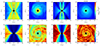 |
Fig. 2. Poloidal (azimuthally averaged) and equatorial plane cuts of selected KHARMA GRMHD simulation snapshots of the two considered accretion modes, both with a* = +0.5. The MAD (left panels) and SANE (right panels) snapshots feature different ion temperatures (displayed in dimensionless units in the upper panels) and the plasma β parameter (displayed in the bottom panels), resulting in different emission properties. The solid black lines represent the σ = 1 surface. The high temperature near the polar axes is a consequence of conservative codes. The temperatures in the polar regions are considered unphysical and are masked out in the radiative transfer calculations (regions with σ > 1 or σ > 3). Here, rg ≡ GM/c2, the gravitational radius. |
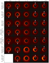 |
Fig. 3. Time-averaged images of all the fiducial models with Rlow = 1 and Rhigh = 40 in the image library. The white arrows indicate the projected direction of the black hole spin for the simulation geometry. The lower left corner is blank because there is no H-AMR SANE a* = −0.94 case in our model library. All images are shown in linear scale. |
Images that include radiation from nonthermal populations of electrons were constructed using the BHAC-BHOSS pipeline. These models have a nonthermal κ distribution, which has a thermal core with a width w that smoothly matches a power-law tail with dne/dγ ∝ γe−κ − 1 for γe ≫ w. The width w was partly determined from the Rlow − Rhigh prescription above, but the model includes a parameter ϵ that represents the fraction of magnetic energy that contributes to the electron acceleration (first introduced by Davelaar et al. 2019; see also Cruz-Osorio et al. 2022; Fromm et al. 2022; Davelaar et al. 2023 for details) and contributes to the width w in a region near an injection radius that we took to be 10 GM/c2. We considered models with ϵ = 0 and 0.5. The parameter κ was determined by β and σ following the prescription of Ball et al. (2018). Example nonthermal models are shown in the fourth and fifth panels in Fig. 3. The image morphology for models with ϵ = 0 (fourth panel) is similar to that of the thermal models (third panel) from the same pipeline. With increasing fraction of nonthermal emission (ϵ = 0.5; fifth panel), the resulting image is more extended, which agrees with Mao et al. (2017), for example.
3.2. Exploratory models
The tilted models were adopted from Chatterjee et al. (2020, see also Liska et al. 2018) and evolved using H-AMR code for a considerably longer time than the fiducial simulations. In tilted models, the accretion flow angular momentum and black hole spin are no longer coaxial, but are instead separated by a tilt angle. We considered tilt angles 0° (as a reference model), 30°, 60°, a single black hole spin (a* = +0.94), and an initial magnetic field setup between the SANE and MAD setup with ϕBH ≈ 7 − 14 (see Chatterjee et al. 2020 for details). The tilted-disk runs adopted Eq. (2) as a prescription for the electron temperatures. The tilted-disk models imaged for one inclination and three azimuthal angles are listed in Table 2. Examples of time-averaged images of tilted disks are shown in Appendix B.
Our library also includes radiative two-temperature models from Chael et al. (2019a) that were simulated using the KORAL-grtrans pipeline. These simulations evolved a two-temperature magnetized fluid and a radiation field as a second fluid, coupled to the plasma using the M1 approximation. These radiative GRMHD (GRRMHD) simulations account for self-consistent radiation physics, incorporating both particle heating and radiative cooling via bremsstrahlung, synchrotron, Compton, and Coulomb losses. Both KORAL simulations in our library are MAD and assume a* = +0.94. The two simulations feature identical initial conditions, but differ in their assumed prescription for subgrid electron heating: turbulent Landau damping (Howes 2010), or magnetic reconnection (Rowan et al. 2017). The radiative simulations were not scale-free. The gas density was scaled to physical units such that the compact emission at 230 GHz is roughly 0.98 Jy which is larger than the 0.5 Jy assumed in the fiducial simulations. This flux normalization was chosen based on pre-EHT constraints on the compact flux, but since the computational cost can be higher by an order of magnitude than a typical fiducial model, we chose not to produce new radiative simulations for this analysis and instead used what was already available. As we discuss in Sect. 4, we only scored on closure quantities, which do not contain information about the total flux. Examples of time-averaged images of radiative models are shown in Appendix B.
3.3. Model uncertainties and library summary
The simulations have several uncertainties that may impact the EHT data interpretation. If the ions and electrons are thermal and the electron temperature Te is lower than the ion temperature Ti, then the ions dominate the pressure. Since the ions are nonrelativistic (kTi/(mic2)< 1), this implies that Γad = 5/3. If Te = Ti, as in Rhigh = 1 models, and in Rlow = 1 models when β ≲ 1, then both components contribute to the pressure, and we can show that Γad = 13/9. Some of our models used Γad = 4/3, but this was purely for numerical convenience because the Γad = 4/3 models are more robust. A change of the adiabatic index in the GRMHD model changes the temperature profile and model images. For example, the KHARMA and H-AMR, MAD or SANE simulations all assumed a different Γad index and therefore do not necessarily have to produce statistically consistent images. Moreover, even when the simulations assumed the same adiabatic index, the radiative transfer codes may interpret it in a different way when they calculate Te (see Appendix H in Sgr A* 2024 VIII). It is therefore possible that even simulations with the same Γad, for instance, the KHARMA and BHAC MAD models, produce different images. Moreover, models with σcut = 3 have slightly lower optical depths (they are slightly brighter and therefore require a smaller density normalization) than the same models with σcut = 1, which introduces another discrepancy. Finally, the initial torus size or the grid resolution may affect the results also to some small degree. The effects of changing the equation of state, σcut, and other parameters in model-data comparisons have yet to be fully investigated, and we therefore treat the variations between the models that are produced by different simulation pipelines as a measure of the model uncertainty. We expect that the same accretion state models produced by different simulation pipelines may not always produce consistent results.
The total number of fiducial model images is ∼170 000 and the total number of images from tilted simulations is ∼10 000, including ∼2000 snapshots of the reference nontilted H-AMR simulation. Our extended image library consists of ∼184 000 snapshots, and it is three times larger than the library assembled in M87* 2017 V.
4. Comparing GRMHD models with data
4.1. Overview of the data selection and comparison
The EHT collected multiple epochs of M87 data in two frequency bands in 2017 and four frequency bands in 2018. We focused our comparisons on the EHT observations centered at 229 GHz (high-band in 2017 and band 4 in 2018). To obtain uncorrelated constraints, we focused our comparisons on two selected days from each campaign: April 6, 2017, and April 21, 2018. April 6, 2017, was chosen following M87* 2017 V based on the highest number of scans in the 2017 datasets and because of the four days of observations in 2017, April 5/6 differ most from the 2018 image. April 21, 2018, was chosen because it has the best (u, v)-coverage in the 2018 campaign. The dynamical timescale of M87∗ near the event horizon (GM/c3 ∼ 9 h) is comparable to the single-epoch observation, and no intra-day variability of M87∗ is therefore expected. The images are expected to be very strongly correlated below timescales of about 50 GM/c3 ∼ 20 days.
To be consistent with M87* 2017 V and M87* 2017 VI, we first compared the models to the observations using two previously developed algorithms: the snapshot scoring, and the average imaging scoring (hereafter, AIS). To effectively perform the scoring procedures on a significant number of model images, a few improvements were made to reduce the computational cost of the calculations. First, we applied an optimization approach instead of the MCMC method with gain fitting (Broderick et al. 2020) (also adopted in M87* 2017 V; M87* 2017 VI). Second, we fit the closure quantities of the VLBI data, such as the closure phases and the closure amplitudes. Third, the scoring was performed with an efficient Julia-based driver developed following Tiede (2022). The snapshot and AIS scoring procedures were performed separately in the 2017 and 2018 observations. In addition to this, we also introduced the multi-epoch scoring, which combines the scoring results for individual observations from different years. Finally, in addition to the EHT constraints of the three aforementioned scoring schemes, the M87 jet power in the models was required to exceed a lower limit of 1042 erg s−1. The following subsections briefly describe each of the scoring schemes and their results. The AIS and multi-epoch scoring methods are described in depth in Appendix C.
4.2. Snapshot scoring constraints
The snapshot scoring approach determines how consistent each model snapshot is with the observation. In this procedure, we fit a given model with the EHT data by rotating and resizing every image in the model to find the best-fit values of the image orientation and the implied mass-to-distance ratio, M/D. The hundreds of images from each model are then used to estimate an ensemble-based posterior.
The mean values of the reduced χ2,  , of the fiducial model fits are ∼10 (for the 2017 datasets) and ∼15–30 (for 2018 datasets). Values much higher than unity are expected because a single model image is unlikely to fit the observation perfectly, given the stochastic character of the turbulence and the finite simulation time. It is expected that the 2018
  values are higher, since the newly added EHT baselines (formed by adding the Greenland Telescope to the EHT network) add more information to the (u, v) domain, while the single-snapshot model retains the same model complexity as in the 2017 analysis.
For exploratory models, the  distributions for the radiative models and tilted-disk models with zero tilt angle are comparable to their distributions from fiducial models. We find that tilted-disk models with a tilt angle of 30° and 60° clearly have much higher values of
  than the other models. This is likely due to the more crescent-like, instead of ring-like, morphology of the tilted images (compare Fig. 3 with Fig. B.1).
Figure 4 shows the posterior distributions M/D for representative fiducial models fit to the 2017 (blue) and 2018 (red) datasets. The distributions shown in Fig. 4 include the results for all geometries available in the image library: for cases where the black hole spin axis pointed away from Earth, and for cases where it pointed toward Earth (see also Table 2). The distributions from different years overlap each other, but the 2018 distributions peak around slightly higher values of M/D for all simulation pipelines. Similar to the result in M87* 2017 V, the distributions for both EHT 2017 and 2018 observations are more consistent with the mass estimation using stellar dynamics studies (e.g. Gebhardt et al. 2011; Liepold et al. 2023; Simon et al. 2024) than with the gas dynamical model (e.g. Walsh et al. 2013).
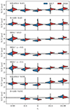 |
Fig. 4. Violin plots for M/D distributions from the snapshot scoring with 2017 and 2018 EHT observations for models with Rlow = 1 and Rhigh = 40 in the image library. The horizontal dashed black line and shaded gray region mark the ranges of M/D = 3.8 ± 0.4 μas reported in M87* 2017 I. |
In Fig. 5 we rotate each snapshot image with its best-fit value of the PA and compare the distribution of the best-fit PAs with the observed forward-jet direction. This rotation is possible based on the prior knowledge of the black hole rotation axis and of the forward-jet axis of each image in our image library, as described in Sect. 3. Figure 5 shows the resulting distribution of the position angles of the models using only the 10% of images with the lowest χν2 from the KHARMA and H-AMR pipelines. We split the models into prograde/retrograde cases and considered both models with a spin axis pointing toward and pointing away from Earth (see discussion in Sect. 3).
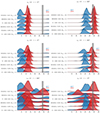 |
Fig. 5. Normalized distributions of the fitted position angle of the forward jet in selected fiducial thermal models based on the snapshot scoring with 2017 and 2018 observations, using the best-fit 10% of the images. The PA = 288° ±10° of the milliarcsecond-scale jet (Walker et al. 2018; Cui et al. 2023) is marked by the vertical dashed black line and shaded gray region. Left: Models with a black hole spin axis or a coordinate system axis (case a* = 0) pointing toward Earth. Prograde cases are shown in the top (a* > 0) and middle (a* = 0) panels, and the retrograde case (a* < 0) is shown in the bottom panel. Right: Models with a black hole spin axis or with a coordinate system axis (case a* = 0) pointing away from Earth. Prograde cases are shown in the top (a* > 0) and middle (for a* = 0 the matter angular momentum is always aligned with the coordinate axis) panels, and the retrograde case (a* < 0) is shown in the bottom panel. See text in this paper or Fig. 5 in M87* 2017 V for a description of the geometry of the black hole axis, flow rotational axis, and inclination angle. |
Figure 5 shows that the jet directions in fiducial models with a black hole spin axis or angular momentum axis (in case of a* = 0) that points away from Earth are significantly better aligned with the large-scale jet position angle (PA = 288° ±10° of the milliarcsecond-scale jet measured by Walker et al. (2018) and Cui et al. (2023), marked with a vertical dashed line) than in the opposite cases. This is true for the 2017 and 2018 scores, but compared to 2017, the 2018 preferred PA distributions are overall significantly better aligned with the large-scale jet. When we assume that the jet axis and black hole spin axis are aligned, our GRMHD simulations imply that the position angle of the brighter side of the ring structure in 2018 (southwest part of the ring) is roughly perpendicular to the jet direction. The distribution functions of the retrograde models are often broader than those of the prograde models, indicating that rings in retrograde models produce a greater angular variability.
The best-fit 2017 PA distributions presented here agree with those reported in M87* 2017 V. The forward-jet PA distributions from the snapshot scoring of the previous smaller model image library from M87* 2017 V is presented in Fig. 20 of Paper I (M87* 2018 I).
4.3. Average imaging scoring constraints
The AIS method aims to determine how likely it is that the EHT data are consistent with a random draw from a specific model image distribution. As demonstrated in the previous subsection (and in M87* 2017 V), individual model snapshots are unlikely to provide an acceptable  fit to the observational data because of the finite number of snapshots and turbulence in the underlying GRMHD simulations.
In M87* 2017 V, we used the AIS scheme to compare the GRMHD models with EHT data that overcome the fluctuations of individual snapshots. The scheme measures the distribution of χν2 distances between individual snapshots and the time-averaged image for each model. This distribution was compared to the distance between the data and the time-averaged image for the same model. The model was then assigned a probability based on where the data lay in the distribution. The model was disfavored when the data lay outside or on the tails of the model distribution.
AIS scoring was applied to all models using both 2017 and 2018 EHT data. We considered models whose 2017 AIS or 2018 AIS probabilities were higher than a certain threshold as equally good. We note that the identification of good models that passed the AIS scoring was based on only two observations, so caution should be taken when interpreting these results. The AIS results for the fiducial models are summarized in the Appendix D. As the threshold for AIS is arbitrary, we present the AIS results for which we chose a probability of 15% or 10% as the threshold5 for passing the models. The AIS scoring results, together with the snapshot scoring results, are necessary ingredients of the multi-epoch scoring procedure introduced next.
4.4. Multi-epoch scoring constraints
The multi-epoch scoring approach aims to provide an odds ratio that computes the probability of the model relative to the probability of the best-performing model. The typical correlated variability time-scale of all the GRMHD simulations (∼30 GM/c3, ∼10 days for M87*) is much shorter than the observational cadence between the EHT 2017 and 2018 observations, and therefore, we can consider the 2017 and 2018 datasets as independent measurements.
In brief, the multi-epoch scoring post-processes the snapshot scoring and AIS scoring results following a Bayesian approach in which AIS results are treated as approximations for Bayesian evidence, and the snapshot scoring results are used as approximations of the ensemble-based posteriors6. The details of the procedure are presented in Appendix C. The odds ratio returned by the multi-epoch scoring provides a measure of the relative preference for two models. In our procedure, the returned odds ratio for a model would be relatively higher if the AIS scores are higher, and the distribution according to the snapshot scoring has a larger overlap (see Eq. (C.16) for a mathematical description). As a result, the multi-epoch scoring is a compromise of how a model could (i) satisfy the 2017 AIS scoring, (ii) satisfy the 2018 AIS scoring, and (iii) explain the 2017 and 2018 observations with same M/D ratio and the same direction of the black hole rotation axis.
An example is given in Fig. 6 as a demonstration of point (iii) in the multi-epoch scoring procedure. In the parameter space of M/D and the PA of forward-jet direction, the overlap of the ensemble posteriors for the 2017 observation and the 2018 observation (indicated by the black contours and profiles) represents how likely the independent observations are to be explained by the same parameters. Points (i) and (ii) mentioned above were also included as conditions when we computed the odds ratio for each model. We then compared the relative odds ratios of the models and selected the models that were preferred by the multi-epoch observations.
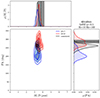 |
Fig. 6. Demonstration of the multi-epoch scoring based on the KHARMA SANE model with (a*, Rlow, Rhigh)=(−0.5, 10, 160). The 2017 and 2018 snapshot scoring results for the given model are shown in the M/D – PA plane with the blue and red distributions, respectively. The larger the overlap between the red and blue distributions, the better the fit of the multi-epoch observations with a single model. The black profile indicates the normalized combined distribution of the best-fit parameters computed according to the multi-epoch scoring procedure (see Sect. 4.4 for details). The dashed lines and shaded areas are the same as explained in Figs. 4 and 5. |
Figure 7 compares the odds ratios for all the models with either black hole spin axes pointing away from Earth or a nonspinning black hole, but the accretion flow spin axis points away from Earth. The scores shown by the vertical axis indicate the relative preference for each model (i.e., the normalized odds ratio according to the specific model with the highest score; therefore, all but one model have relative scores lower than 100%). We selected 1% of the normalized odds ratio as the arbitrary threshold for the passing models. The low threshold value is motivated by all the uncertainties associated with the modeling of the images.
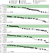 |
Fig. 7. Overview of the multi-epoch scoring results for all the fiducial models with black hole axes pointing away from Earth, and nonspinning black holes with a inclination angle i = 163°. The y-axis is the normalized odds ratio (see text for details), which indicates the relative preference by multi-epoch (2017 and 2018) observations. Models with different spins are shown in different panels. The green region marks passing models for which the relative odds ratio is ≥1%. Models with a relative odds ratio ≤0.001% are not shown. |
Figure 7 shows models from all three pipelines with high relative scores, and MAD models reach higher scores overall than SANE models. Moreover, the multi-epoch scoring rules out more of the prograde models than the retrograde models. This can be explained by the more turbulent character of the retrograde models, which results in broader PA distributions, as shown in Fig. 5, and a better overlap between two observational epochs. Interestingly, tilted-disk models (which have positive black hole spins a* = +0.94) have relatively low scores. The models that passed multi-epoch scoring were further combined with jet-power constraints.
4.5. Jet-power constraint
Previous studies of M87 estimated its jet power to be Pjet = 1042 − 1045 erg s−1 (Reynolds et al. 1996; Li et al. 2009; de Gasperin et al. 2012; Broderick & Tchekhovskoy 2015; Prieto et al. 2016). Following M87* 2017 V, we computed the powers of outflows in our GRMHD simulations and compared them with observations. We adopted the same criterion as in previous EHT publications for the failing models with an insufficient jet power, that is, a model fails when its outward energy flux (outflow power; Pout) over the black hole polar regions is lower than 1042 erg s−1.
In our models, the Δt-averaged Pout is defined as
 (3)
(3)
where Ttr is a component of the stress-energy tensor associated with the outward radial energy flux, and ρur subtracts the rest-mass energy flux, g is the metric determinant, ur is the gas four-velocity in radial direction, and the other variables have their usual meaning. In Eq. (3), ϕ and θ are the azimuthal and polar angles, respectively, and we only included those θ whose time- and azimuth-averaged energy flux was directed outward. There are many choices to define the cut on the polar region to integrate only sufficiently relativistic outflows, for example, a cut based on βγ, or the Bernoulli parameter values. Here, the polar angle integration includes 1 radian about the north or south poles and only those regions whose energy flux is directed outward. This includes both the relativistic narrow jet near the polar axis and a portion of the nonrelativistic outflows at higher inclinations. Pout can therefore be larger than the Blandford-Znajek jet power associated with the relativistic part of the jet, and models with zero spin may have Pout > 0. In some cases, for instance, SANEs, the Pout measurement can be dominated by the nonrelativistic outflows. Pout also depends on the selected mass unit (ℳ), which was used to set the ∼230 GHz total flux, overall density, and magnetic field strength in the simulations. Therefore, models with very cold electrons will have higher ℳ and proportionally higher Pout. However, the variations in Pout in the imaging parameters (inclination and R − β prescription) are smaller than the variations in the GRMHD simulation parameters (spin and accretion mode). For all of the fiducial models, Pout is a strong function of |a*|.
The jet-power scoring results for the fiducial MAD and SANE models are shown in combination with the multi-epoch scoring in Table 3. For all codes, the a* = 0 MAD models fail the power constraint most often (16 out of 20 fail). SANE models with Rhigh = 1 also often fail, regardless of spin. These results are consistent with those reported in M87* 2017 V. Pout in the fiducial nonthermal MAD models show the same trend as in the fiducial thermal models, but all a* = 0 MAD models fail. All spinning nonthermal MAD models pass the jet-power constraint.
Pass and fail table for the fiducial models.
For exploratory models, all tilted models pass the jet power constraint. This is an expected result as the tilted models assumed high spins (a* = +0.94), for which most of the aligned fiducial models pass as well (with the exception of the few aforementioned SANEs). In addition, both high-spin radiative MAD models produce jet powers of Pjet ∼ 1043 erg s−1 (see Table 1 of Chael et al. 2019b), and thus, they pass the jet-power constraint7.
5. Discussion
5.1. Summary of the model constraints and best-bet models
Table 3 displays the pass and fail information for fiducial models in which their black hole spin axes point away from Earth, or, when the black hole is nonrotating, the flow spin axes point away from Earth. As discussed in Sect. 4.2, models oriented in this way are more probable given the direction of the large-scale jet in M87∗, assuming a coaxial model. The pass and fail table combines two constraints: the multi-epoch scoring, and the jet power. Models that pass (or fail) these two constraints are indicated by dark green (or yellow), and models that pass only one constraint are indicated by other colors. We refer to the models that pass both constraints as the best-bet models. The exploratory models (all with a* = 0.94) are not shown in Table 3: The two radiative models are also among the best-bet models, but all tilted disks have a relatively low multi-epoch score below the chosen cutoff. For reference, the M/D distributions for radiative models are presented in Appendix E. The M/D distributions for tilted-disk models are not shown since these models in general have higher  (see Sect. 4.2), and they perform poorly in all other scoring constraints.
Most of the best-bet models pass both the 2017 AIS and 2018 AIS scoring, as expected from the multi-epoch scoring introduced in Sect. 4.4. Most models that fail both 2017 AIS and 2018 AIS also fail the multi-epoch scoring (see also Table D.1). However, some models pass both the 2017 AIS and 2018 AIS scoring, but fail the multi-epoch scoring because the multi-epoch scoring returns an odds ratio that depends not only on AIS scoring, but also on a constant M/D and PA to explain the observation. This demonstrates that our multi-epoch scoring procedure is more powerful than a logical AND applied to the 2017 AIS and 2018 AIS scoring results alone. For the jet-power constraints, models with a* = 0 are generally less favored than spinning models.
The 68 best-bet models of the 194 fiducial models are shown in Table 3. The best-bet models include all types of fiducial models: thermal MAD and SANE models, and nonthermal MADs. However, the survival rate for MADs is higher than that for SANEs. For certain spins, the survival rate of the nonthermal MAD models does not strongly depend on the details of nonthermal physics (e.g., models with ϵ = 0 and ϵ = 0.5 score similarly for a* = ( − 0.95, −0.5, 0)). Among all the best-bet models, retrograde models have a relatively higher survival rate than all other cases. We propose that turbulence might account for the variation in the brightest segment of the ring-like structure. This conjecture finds further support in the fact that retrograde models, characterized by higher levels of turbulence near the event horizon compared to prograde models (see also Fig. 5, where the PA distributions in retrograde models are often broader than in prograde models), match the observations better. In addition, the M/D distribution for 2017 and 2018 shown in Fig. 4 also overlaps better for negative spin cases.
Not all pipelines exhibit the same pass and fail results across the flow type, spin, and thermal electron parameters. For example, the KHARMA MAD, a* = +0.94, Rlow = 1, Rhigh = 1 model only passes the jet-power constraint, while the H-AMR model with the same parameters passes both the jet power and multi-epoch scoring constraints. The discrepancy may be due to differences in the numerical scheme in the code itself, to the simulation setup, and to post-processing details (see Tables 1 and 2). The models are also subject to sampling errors: the snapshots are drawn from a limited number of correlation times, meaning that acceptable models may be occasionally rejected.
Table 3 also demonstrates that the multi-epoch observations provide more constraining power, because more models fail only the multi-epoch-constraints than fail only the jet constraint. In M87* 2017 V, AIS scoring based on the 2017 M87∗ EHT observation was applied as one of the constraints for the model selection. This single-year EHT constraint has less constraining power than the jet-power constraint (see Table 2 of M87* 2017 V). That is, the jet-power constraint can rule out more models than are ruled out by the 2017 AIS results. With the multi-year M87∗ EHT observations, based on Stokes I properties of the model images, we were able to provide EHT constraints with a relative more constraining power than the jet-power constraints. The increased constraining power with multi-year observations is closely related to the fact that the ring in M87∗ looks substantially different in 2017 and 2018.
Our exploratory models are sampled more sparsely than the fiducial models. There is a larger parameter space left to be explored for these models in the future (e.g., they currently all have spin a* = +0.94). A more comprehensive radiative image library from two-temperature GRRMHD simulations with different black hole spins and flow types would be valuable considering the relatively good performance in this scoring. In the tilted models, even the reference zero tilt-angle model is not selected as one of the best-bet models. We recall that the tilted simulations have an intermediate magnetic flux between MAD and SANE, and therefore, the zero-tilt exploratory model is distinct from any of the fiducial models.
5.2. Multiwavelength spectra of the selected best-bet models
We determined whether the best-bet models are consistent with the multi-wavelength observations of M87∗. We calculated broadband spectral energy distributions (SEDs) for a few selected best-bet thermal synchrotron models. In Fig. 8 we present the SEDs for three best-bet models along with radio and X-ray observations collected in 2018 (EHT MWL Science Working Group 2024). The selected models are taken from the KHARMA pipeline. They include SANE with (a*, Rlow, Rhigh)=(0.94, 10, 160), SANE with (a*, Rlow, Rhigh)=(−0.5, 1, 160), and MAD with (a*, Rlow, Rhigh)=(−0.5, 10, 40). The SEDs were generated using the Monte Carlo relativistic radiative transfer code grmonty (Dolence et al. 2009), which includes synchrotron (emission and self-absorption), inverse-Compton scattering, and bremsstrahlung emission. In the EHT bands, the emission is dominated by the synchrotron process. The X-ray part of the SED is dominated by either Compton upscattering of synchrotron photons or by bremsstrahulung emission. In general, both the Compton and bremsstrahulung components are relatively more prominent in SANEs than in MADs. The observed X-ray emission can be contributed by scales that far exceed the size of our model (EHT MWL Science Working Group 2024). When we treat the observed X-ray luminosity as an upper limit for the models, the best-bet models shown in Fig. 8 are all acceptable. Among the three SEDs, the time-averaged X-ray emission of one of the SANE models,(a*, Rlow, Rhigh)=(0.94, 10, 160), matches the observations, but in this case, the synchrotron peak is at much higher frequency than in the EHT bands. We also note that the flux in the optical and X-ray bands may increase when the nonthermal synchrotron component is considered as well.
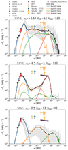 |
Fig. 8. Time-averaged SEDs of selected best-bet models. The data points are taken from the multi-wavelength observations during the 2018 EHT campaign (EHT MWL Science Working Group 2024). The EHT observation is marked by the vertical red bar. The gray region of the SED indicates the variations of the SED for different snapshots. The colored histograms correspond to different radiative processes: synchrotron emission (blue), synchrotron photons scattered once (orange), synchrotron photons scattered twice (green), and bremsstrahlung (red). The total emission is displayed in black. |
5.3. Mass-to-distance ratios and implications for gravitational physics
As discussed in Sect. 4.2, models in which the black-hole spin axis points away from Earth together with nonspinning black holes with an inclination angle i = 163° are preferred by both 2017 and 2018 observations. In Fig. 9 we show the mass-to-distance ratio (M/D) distributions for each GRMHD pipeline and for all pipelines combined. These distributions only include the top 10% best χ2 images from the snapshot scoring procedure. The 2017 and 2018 constraints are represented with the blue and red distributions, respectively. For each model library, the 2018 results (red distribution) prefer slightly higher values for M/D than the results from the 2017 observations (blue distribution). This preference for a slightly higher value for M/D is consistent with the results from the image reconstructions in Paper I (M87* 2018 I), which prefer slightly larger diameters and slightly smaller ring widths for the 2018 data. The 2018 data prefer  , and the 2017 data prefer an
  . When we convert the above M/D values into units of solar masses at a distance of 16.8 Mpc, the mass for M87∗ using the updated 2018 EHT observations is
  , and it is
  for the 2017 observations.
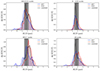 |
Fig. 9. Distribution of M/D obtained by fitting the 2017 (blue) and 2018 (red) data with the fiducial models shown in Table 3. These distributions are generated from the top 10% best-fitting snapshots by χ2. The results for models prepared by the KHARMA, H-AMR, and BHACpipelines are shown separately, together with the result for all the models combined. The distribution when combining both the 2017 and 2018 result by the multi-epoch scoring algorithm is shown as the black profile. The vertical dashed black line and shaded gray region mark the ranges of M/D = 3.8 ± 0.4 μas reported in Event Horizon Telescope Collaboration (2019a). |
Applying the multi-epoch scoring algorithm, we also constructed a combined M/D distribution (black distribution) for all the fiducial models (see also Fig. 6 for comparison). The combined distribution prefers an  (
( ). We summarize the mass estimates from the individual years and the multi-epoch results in Table 4. The slightly lower mass estimate when incorporating the multi-epoch constraints can be attributed to the general preference for retrograde models in the scoring results. The retrograde models generally produce less compact images, so that the snapshot scoring procedure tends to shrink the simulated images to match the size of the emission region in the real data, leading to lower mass estimates. This bias may disappear in the future when we also incorporate additional conditions in the image structure in the snapshot scoring procedure beyond rescaling and rotation. Dedicated image reconstruction techniques may also be able to incorporate a more complicated image structure and differentiate between models with less compact emission. These new M/D values are statistically consistent with the result published in 2019, that is,
  (M87* 2017 I; M87* 2017 VI), and it differs by about 1.5 − 2σ from the mass estimates made in Liepold et al. (2023) and by slightly more than 1σ from the mass estimates found in Simon et al. (2024).
Summary of M/D and M estimates.
Notwithstanding the slight differences between the new mass estimate and that published in 2019, it is also important not to overinterpret them. Numerous changes have been introduced to the GRMHD pipelines since the 2019 analysis, as described in Sect. 3, and it is expected that the new library produces some differences from the previous library in the mass estimate. Even within the new model library, significant differences remain between the model pipelines beyond the black hole spin, electron temperature prescription, and magnetic field configuration that change the M/D distributions. In addition, the coarse sampling of these parameters within a given pipeline can produce significant spikes in the multi-epoch M/D distributions that come from a small number of high-performing models (see, e.g., the black KHARMA curve). Nevertheless, when we consider either the new individual or the combined mass estimates, the differences between the M87* 2017 VI result and the mass results presented in this work are not statistically significant. In view of this, we regard the new M/D and mass estimates to be consistent with those published in the 2019 papers (M87* 2017 I; M87* 2017 VI). As anticipated above, this conclusion is also expected when we assume that M87∗ is a supermassive black hole described by general relativity, whose corresponding spacetime is either static or stationary, and hence cannot exhibit a significant difference in its properties over a timescale of only one year.
6. Conclusions
In M87* 2018 I, we presented the results of the 2018 EHT observations of M87∗ at 1.3 mm. Leveraging the first 2017 and the newest 2018 EHT observations of M87∗, we here compared the source Stokes I observations to the upgraded library of GRMHD simulations of black hole accretion. The new model library consists of fiducial thermal synchrotron emission models and compares for the first time tilted-disk models and radiative GRMHD models.
First, treating 2017 and 2018 observations as independent experiments, we presented the results of the snapshot scoring and average image scoring (AIS) procedures. Assuming that the black hole angular momentum axis is aligned with the jet axis, we find that the observations prefer a spin axis of the black hole that points away from Earth.
Next, we presented a Bayesian-based multi-epoch scoring procedure, within which the AIS results were used to approximate the Bayesian evidence, and the snapshot scoring results were used to approximate the ensemble-based posterior construction. In the multi-epoch scoring algorithm, the success of a model is also evaluated based on whether the same M/D ratio and black hole rotation axis in the model is consistent with both years of data. As a result, the multi-epoch scoring was performed as a post-processing step using the results of both the snapshot and AIS procedures. The multi-epoch scoring produces better constraints than the single-year scoring, for instance, the AIS scoring alone. The multi-epoch scoring finds that retrograde models have a higher survival rate than prograde systems, which might be related to their comparatively more turbulent nature. The main cause of the stronger variability of the retrograde flows may require further examinations. For example, the variability in the PA in the retrograde flows does not seem to be correlated with the accretion rate onto the black hole (Narayan et al. 2022).
The current analysis does not allow us to explain the M87 flaring in VHE reported in EHT MWL Science Working Group (2024) with the near horizon emission because passing purely thermal models do not produce emission at these energies. Future simultaneous observations at higher frequencies (∼THz) could help us to distinguish an accretion state or black hole spin in M87∗ probably only for the nonthermal models.
The recent reanalysis of historical radio (86 GHz) observations of the M87 core indicated a quasi-periodic change in the 288° position angle of the large-scale jet by about 10° degrees with a period of 11 years (Cui et al. 2023). The tilted models were disfavored in this work, but current results do not yet have significant implications for the jet precession. A correlation of the jet motion with the variation in the horizon-scale structure would require many more EHT epochs, together with low-frequency VLBI monitoring, preferably sampling timescales shorter than one year. Nevertheless, for future tilted model simulations, it would be useful to explore the effect of a tilted accretion flow around black holes with various spins and with a wider range of tilt angles.
The sensitivities of the 2017 and 2018 EHT arrays are insufficient to reveal jet-related extended emission near the black hole with confidence (e.g. Broderick et al. 2022), although future EHT observations for M87∗ with adequate dynamical range may show further details of an extended component in addition to the near-horizon ring structure. In this case, several emission features related to the jet physics may also be tested and constrained (e.g. Broderick & Tchekhovskoy 2015; Pu et al. 2017; Jeter et al. 2020). We also note that including the morphology constraint of M87∗ at lower frequencies can aid in identifying the relative contributions of the emission from the accretion and jet components of M87∗ (Lu et al. 2023), which would otherwise be challenging if based on the SED alone (Dexter et al. 2012).
Regardless of all these limitations, our current models can be still further constrained by their polarimetric properties (see, e.g., M87* 2017 VII; M87* 2017 VIII or M87* 2017 IX). We postpone a full discussion of the multi-epoch polarimetric scoring to a forthcoming publication.
When we assume that the black hole spin axis is closely aligned with the large-scale jet axis, images of the black hole shadow from GRMHD simulations produce a distribution of brightness position angles centered roughly 90° offset from the jet position angle. If this is the case, then the brightness position angle of the 2017 images should be relatively rare when making many independent observations. For this reason, we predicted in the previous paper series (M87* 2017 V) that future observations would most likely show a brightness position angle counterclockwise from the 2017 value. The 2018 observations appear to follow this prediction, but only represent one additional independent realization. The current multi-epoch analysis was performed on just two years of data, so that any differences between the years may be subject to concerns about small-number statistics. Future observations can help us to build confidence in our results. The analysis of the EHT data from later years (2021 and 2022) are already underway and will help us understand whether the brightness position angle of the 2017 observations is rare, following our predictions. In addition, a proper distribution of the brightness position angles in the observations can be a powerful tool for constraining the simulations by helping us reject simulations that return distributions of the position angle that are too wide or too narrow.
While the year-to-year analysis of EHT images is critical for understanding the uncorrelated variability of M87∗, a dedicated monitoring campaign consisting of observations every few days over the course of one to two months is necessary to investigate the correlated variability around M87∗. Observations with this high cadence would provide correlated constraints, unlike the independent constraints from the year-scale observation cadence considered in this paper. The EHT observations already revealed differences between the correlated variability seen in current GRMHD simulations and the variability seen in Sgr A* (the simulated variability is typically stronger than the observed variability in the total-intensity light curves; see Wielgus et al. (2022) and Sgr A* 2017 V for further discussion), and a dedicated effort to investigate the correlated variability in M87∗ will provide an independent constraint and valuable cross-check on models for the magnetic field and turbulent plasma environment around the black hole.
The angular size of a nonrotating black hole shadow on the sky is  , where G is the gravitational constant, M is the black hole mass, c is the speed of light, and D is the distance to the black hole. Assuming a black hole mass M = 6.5 × 10⁹ M⊙ at a distance of D = 16.9 Mpc, we obtain dsh ≈ 39.75 μas.
The ϕBH values mentioned here are computed in Heaviside units, in which a factor of  is absorbed within B.
The radiative models assumed MBH = 6.2 × 10⁹ M⊙ at a distance of D = 16.2 Mpc, and an observational frequency of 230 GHz.
The radiative models had a field of view of ≈25 GM/c2 × 25 GM/c2 (≈100 μas × 100 μas), and the resolution was 512 × 512 pixels.
The choice of the threshold does not affect the multi-epoch scoring result presented in Sect. 4.4.
For posterior estimations for each model, we considered the best 10% images according the snapshot scoring results.
Chael et al. (2019b) measured the jet power at a radius r = 100rg over the polar region with a Bernoulli parameter Be < 0.05 (Narayan et al. 2012). This region subtends by less than 1 radian, so that the jet powers reported in Chael et al. (2019b) are generally lower than the outflow power (Eq. (3)).
By simulation we will mean a single GRMHD simulation at a specified black hole spin, observed from a specified orientation, with a specified radiative transfer model (e.g., Rhigh, etc.).
Acknowledgments
The full acknowledgements are available in Appendix A.
References
- Aharonian, F., Akhperjanian, A. G., Bazer-Bachi, A. R., et al. 2006, Science, 314, 1424 [Google Scholar]
- Akiyama, K., Alberdi, A., Alef, W., et al. 2023, ApJ, 957, L20 [NASA ADS] [CrossRef] [Google Scholar]
- Balbus, S. A., & Hawley, J. F. 1991, ApJ, 376, 214 [Google Scholar]
- Ball, D., Özel, F., Psaltis, D., Chan, C.-K., & Sironi, L. 2018, ApJ, 853, 184 [NASA ADS] [CrossRef] [Google Scholar]
- Bardeen, J. M. 1973 Black Holes (Les Astres Occlus), 215 [Google Scholar]
- Bisnovatyi-Kogan, G. S., & Ruzmaikin, A. A. 1974, Ap&SS, 28, 45 [NASA ADS] [CrossRef] [Google Scholar]
- Blandford, R. D., & Payne, D. G. 1982, MNRAS, 199, 883 [CrossRef] [Google Scholar]
- Blandford, R. D., & Znajek, R. L. 1977, MNRAS, 179, 433 [NASA ADS] [CrossRef] [Google Scholar]
- Broderick, A. E., & Loeb, A. 2009, ApJ, 697, 1164 [NASA ADS] [CrossRef] [Google Scholar]
- Broderick, A. E., & Tchekhovskoy, A. 2015, ApJ, 809, 97 [NASA ADS] [CrossRef] [Google Scholar]
- Broderick, A. E., Gold, R., Karami, M., et al. 2020, ApJ, 897, 139 [Google Scholar]
- Broderick, A. E., Pesce, D. W., Gold, R., et al. 2022, ApJ, 935, 61 [NASA ADS] [CrossRef] [Google Scholar]
- Chael, A., Narayan, R., & Johnson, M. D. 2019a, MNRAS, 486, 2873 [NASA ADS] [CrossRef] [Google Scholar]
- Chael, A. A., Bouman, K. L., Johnson, M. D., et al. 2019b, Astrophysics Source Code Library [record ascl:1904.004] [Google Scholar]
- Chael, A., Bouman, K., Johnson, M., et al. 2019c, https://doi.org/10.5281/zenodo.2614016 [Google Scholar]
- Chatterjee, K., & Narayan, R. 2022, ApJ, 941, 30 [NASA ADS] [CrossRef] [Google Scholar]
- Chatterjee, K., Younsi, Z., Liska, M., et al. 2020, MNRAS, 499, 362 [NASA ADS] [CrossRef] [Google Scholar]
- Cruz-Osorio, A., Fromm, C. M., Mizuno, Y., et al. 2022, Nat. Astron., 6, 103 [NASA ADS] [CrossRef] [Google Scholar]
- Cui, Y. Z., Hada, K., Kawashima, T., et al. 2023, https://doi.org/10.21203/rs.3.rs-2624984/v1 [Google Scholar]
- Davelaar, J., Olivares, H., Porth, O., et al. 2019, A&A, 632, A2 [NASA ADS] [CrossRef] [EDP Sciences] [Google Scholar]
- Davelaar, J., Ripperda, B., Sironi, L., et al. 2023, ApJ, 959, L3 [NASA ADS] [CrossRef] [Google Scholar]
- de Gasperin, F., Orrú, E., Murgia, M., et al. 2012, A&A, 547, A56 [NASA ADS] [CrossRef] [EDP Sciences] [Google Scholar]
- De Villiers, J.-P., Hawley, J. F., & Krolik, J. H. 2003, ApJ, 599, 1238 [NASA ADS] [CrossRef] [Google Scholar]
- Dexter, J. 2016, MNRAS, 462, 115 [CrossRef] [Google Scholar]
- Dexter, J., Agol, E., Fragile, P. C., & McKinney, J. C. 2010, ApJ, 717, 1092 [NASA ADS] [CrossRef] [Google Scholar]
- Dexter, J., McKinney, J. C., & Agol, E. 2012, MNRAS, 421, 1517 [NASA ADS] [CrossRef] [Google Scholar]
- Dolence, J. C., Gammie, C. F., Mościbrodzka, M., & Leung, P. K. 2009, ApJS, 184, 387 [NASA ADS] [CrossRef] [Google Scholar]
- EHT MWL Science Working Group (Algaba, J. C., et al.) 2021, ApJ, 911, L11 [NASA ADS] [CrossRef] [Google Scholar]
- EHT MWL Science Working Group (Algaba, J. C., et al.) 2024, A&A, 692, A140 [NASA ADS] [CrossRef] [EDP Sciences] [Google Scholar]
- Event Horizon Telescope Collaboration (Akiyama, K., et al.) 2019a, ApJ, 875, L1 (M87* 2017 I) [Google Scholar]
- Event Horizon Telescope Collaboration (Akiyama, K., et al.) 2019b, ApJ, 875, L2 (M87* 2017 II) [Google Scholar]
- Event Horizon Telescope Collaboration (Akiyama, K., et al.) 2019c, ApJ, 875, L3 (M87* 2017 III) [Google Scholar]
- Event Horizon Telescope Collaboration (Akiyama, K., et al.) 2019d, ApJ, 875, L4 (M87* 2017 IV) [Google Scholar]
- Event Horizon Telescope Collaboration (Akiyama, K., et al.) 2019e, ApJ, 875, L5 (M87* 2017 V) [Google Scholar]
- Event Horizon Telescope Collaboration (Akiyama, K., et al.) 2019f, ApJ, 875, L6 (M87* 2017 VI) [Google Scholar]
- Event Horizon Telescope Collaboration (Akiyama, K., et al.) 2021a, ApJ, 910, L12 (M87* 2017 VII) [Google Scholar]
- Event Horizon Telescope Collaboration (Akiyama, K., et al.) 2021b, ApJ, 910, L13 (M87* 2017 VIII) [Google Scholar]
- Event Horizon Telescope Collaboration (Akiyama, K., et al.) 2022, ApJ, 930, L16 (Sgr A* 2017 V) [NASA ADS] [CrossRef] [Google Scholar]
- Event Horizon Telescope Collaboration (Akiyama, K., et al.) 2024, A&A, 681, A79 (M87* 2018 I) [NASA ADS] [CrossRef] [EDP Sciences] [Google Scholar]
- Falcke, H., Melia, F., & Agol, E. 2000, ApJ, 528, L13 [Google Scholar]
- Fishbone, L. G., & Moncrief, V. 1976, ApJ, 207, 962 [NASA ADS] [CrossRef] [Google Scholar]
- Fromm, C. M., Cruz-Osorio, A., Mizuno, Y., et al. 2022, A&A, 660, A107 [NASA ADS] [CrossRef] [EDP Sciences] [Google Scholar]
- Gammie, C. F., McKinney, J. C., & Tóth, G. 2003, ApJ, 589, 444 [Google Scholar]
- Gebhardt, K., Adams, J., Richstone, D., et al. 2011, ApJ, 729, 119 [Google Scholar]
- Gelles, Z., Chatterjee, K., Johnson, M., Ripperda, B., & Liska, M. 2022, Galaxies, 10, 107 [NASA ADS] [CrossRef] [Google Scholar]
- Gold, R., Broderick, A. E., Younsi, Z., et al. 2020, ApJ, 897, 148 [Google Scholar]
- Hakobyan, H., Ripperda, B., & Philippov, A. A. 2023, ApJ, 943, L29 [Google Scholar]
- Hilbert, D. 1917, Nachrichten von der Königlichen Gesellschaft der Wissenschaften zu Göttingen - Mathematisch-physikalische Klasse (Berlin: Weidmannsche Buchhandlung), 53 [Google Scholar]
- Howes, G. G. 2010, MNRAS, 409, L104 [NASA ADS] [Google Scholar]
- Ichimaru, S. 1977, ApJ, 214, 840 [NASA ADS] [CrossRef] [Google Scholar]
- Igumenshchev, I. V., Narayan, R., & Abramowicz, M. A. 2003, ApJ, 592, 1042 [Google Scholar]
- Jaroszynski, M., & Kurpiewski, A. 1997, A&A, 326, 419 [Google Scholar]
- Jeter, B., Broderick, A. E., & Gold, R. 2020, MNRAS, 493, 5606 [CrossRef] [Google Scholar]
- Jia, H., Ripperda, B., Quataert, E., et al. 2023, MNRAS, 526, 2924 [NASA ADS] [CrossRef] [Google Scholar]
- Koide, S., Meier, D. L., Shibata, K., & Kudoh, T. 2000, ApJ, 536, 668 [Google Scholar]
- Kunz, M. W., Schekochihin, A. A., & Stone, J. M. 2014, Phys. Rev. Lett., 112, 205003 [NASA ADS] [CrossRef] [Google Scholar]
- Li, Y.-R., Yuan, Y.-F., Wang, J.-M., Wang, J.-C., & Zhang, S. 2009, ApJ, 699, 513 [NASA ADS] [CrossRef] [Google Scholar]
- Liepold, E. R., Ma, C.-P., & Walsh, J. L. 2023, ApJ, 945, L35 [NASA ADS] [CrossRef] [Google Scholar]
- Liska, M., Hesp, C., Tchekhovskoy, A., et al. 2018, MNRAS, 474, L81 [Google Scholar]
- Liska, M. T. P., Chatterjee, K., Issa, D., et al. 2022, ApJS, 263, 26 [NASA ADS] [CrossRef] [Google Scholar]
- Lu, R.-S., Asada, K., Krichbaum, T. P., et al. 2023, Nature, 616, 686 [CrossRef] [Google Scholar]
- Luminet, J. P. 1979, A&A, 75, 228 [Google Scholar]
- Lynden-Bell, D. 2006, MNRAS, 369, 1167 [NASA ADS] [CrossRef] [Google Scholar]
- Mao, S. A., Dexter, J., & Quataert, E. 2017, MNRAS, 466, 4307 [NASA ADS] [Google Scholar]
- Mościbrodzka, M., & Gammie, C. F. 2018, MNRAS, 475, 43 [CrossRef] [Google Scholar]
- Mościbrodzka, M., Falcke, H., & Shiokawa, H. 2016, A&A, 586, A38 [Google Scholar]
- Mościbrodzka, M., Janiuk, A., & De Laurentis, M. 2021, MNRAS, 508, 4282 [CrossRef] [Google Scholar]
- Narayan, R., & Yi, I. 1994, ApJ, 428, L13 [Google Scholar]
- Narayan, R., & Yi, I. 1995, ApJ, 452, 710 [NASA ADS] [CrossRef] [Google Scholar]
- Narayan, R., Igumenshchev, I. V., & Abramowicz, M. A. 2003, PASJ, 55, L69 [NASA ADS] [Google Scholar]
- Narayan, R., Sądowski, A., Penna, R. F., & Kulkarni, A. K. 2012, MNRAS, 426, 3241 [Google Scholar]
- Narayan, R., Chael, A., Chatterjee, K., Ricarte, A., & Curd, B. 2022, MNRAS, 511, 3795 [NASA ADS] [CrossRef] [Google Scholar]
- Penna, R. F., Kulkarni, A., & Narayan, R. 2013, A&A, 559, A116 [NASA ADS] [CrossRef] [EDP Sciences] [Google Scholar]
- Pordes, R., Petravick, D., Kramer, B., et al. 2007, J. Phys. Conf. Ser., 78, 012057 [NASA ADS] [CrossRef] [Google Scholar]
- Porth, O., Olivares, H., Mizuno, Y., et al. 2017, Comput. Astrophys. Cosmol., 4, 1 [Google Scholar]
- Porth, O., Chatterjee, K., Narayan, R., et al. 2019, ApJS, 243, 26 [Google Scholar]
- Prather, B. 2022, Thesis, University of Illinois at Urbana-Champaign, USA [Google Scholar]
- Prather, B. S., Dexter, J., Moscibrodzka, M., et al. 2023, ApJ, 950, 35 [NASA ADS] [CrossRef] [Google Scholar]
- Prieto, M. A., Fernández-Ontiveros, J. A., Markoff, S., Espada, D., & González-Martín, O. 2016, MNRAS, 457, 3801 [NASA ADS] [CrossRef] [Google Scholar]
- Pu, H.-Y., Wu, K., Younsi, Z., et al. 2017, ApJ, 845, 160 [NASA ADS] [CrossRef] [Google Scholar]
- Rees, M. J., Begelman, M. C., Blandford, R. D., & Phinney, E. S. 1982, Nature, 295, 17 [CrossRef] [Google Scholar]
- Reynolds, C. S., Di Matteo, T., Fabian, A. C., Hwang, U., & Canizares, C. R. 1996, MNRAS, 283, L111 [CrossRef] [Google Scholar]
- Ripperda, B., Liska, M., Chatterjee, K., et al. 2022, ApJ, 924, L32 [NASA ADS] [CrossRef] [Google Scholar]
- Rowan, M. E., Sironi, L., & Narayan, R. 2017, ApJ, 850, 29 [NASA ADS] [CrossRef] [Google Scholar]
- Sadowski, A., Narayan, R., Tchekhovskoy, A., & Zhu, Y. 2013, MNRAS, 429, 3533 [CrossRef] [Google Scholar]
- Sądowski, A., Wielgus, M., Narayan, R., et al. 2017, MNRAS, 466, 705 [NASA ADS] [CrossRef] [Google Scholar]
- Sfiligoi, I., Bradley, D. C., Holzman, B., et al. 2009, 2009 WRI World Congress on Computer Science and Information Engineering, 2, 428 [CrossRef] [Google Scholar]
- Simon, D. A., Cappellari, M., & Hartke, J. 2024, MNRAS, 527, 2341 [Google Scholar]
- Tchekhovskoy, A., Narayan, R., & McKinney, J. C. 2011, MNRAS, 418, L79 [NASA ADS] [CrossRef] [Google Scholar]
- Tiede, P. 2022, J. Open Source Softw., 7, 4457 [NASA ADS] [CrossRef] [Google Scholar]
- Walker, R. C., Hardee, P. E., Davies, F. B., Ly, C., & Junor, W. 2018, ApJ, 855, 128 [Google Scholar]
- Walsh, J. L., Barth, A. J., Ho, L. C., & Sarzi, M. 2013, ApJ, 770, 86 [NASA ADS] [CrossRef] [Google Scholar]
- Wielgus, M., Akiyama, K., Blackburn, L., et al. 2020, ApJ, 901, 67 [Google Scholar]
- Wielgus, M., Marchili, N., Martí-Vidal, I., et al. 2022, ApJ, 930, L19 [NASA ADS] [CrossRef] [Google Scholar]
- Wong, G. N., Prather, B. S., Dhruv, V., et al. 2022, ApJS, 259, 64 [NASA ADS] [CrossRef] [Google Scholar]
- Younsi, Z., Wu, K., & Fuerst, S. V. 2012, A&A, 545, A13 [NASA ADS] [CrossRef] [EDP Sciences] [Google Scholar]
- Younsi, Z., Porth, O., Mizuno, Y., Fromm, C. M., & Olivares, H. 2020, in Perseus in Sicily: From Black Hole to Cluster Outskirts, eds. K. Asada, E. de Gouveia Dal Pino, M. Giroletti, H. Nagai, & R. Nemmen, 342, 9 [Google Scholar]
Appendix A: Acknowledgements
We thank the anonymous referee for helpful comments that improved the paper.
The Event Horizon Telescope Collaboration thanks the following organizations and programs: the Academia Sinica; the Academy of Finland (projects 274477, 284495, 312496, 315721); the Agencia Nacional de Investigación y Desarrollo (ANID), Chile via NCN19_058 (TITANs), Fondecyt 1221421 and BASAL FB210003; the Alexander von Humboldt Stiftung; an Alfred P. Sloan Research Fellowship; Allegro, the European ALMA Regional Centre node in the Netherlands, the NL astronomy research network NOVA and the astronomy institutes of the University of Amsterdam, Leiden University, and Radboud University; the ALMA North America Development Fund; the Astrophysics and High Energy Physics programme by MCIN (with funding from European Union NextGenerationEU, PRTR-C17I1); the Black Hole Initiative, which is funded by grants from the John Templeton Foundation (60477, 61497, 62286) and the Gordon and Betty Moore Foundation (Grant GBMF-8273) - although the opinions expressed in this work are those of the author and do not necessarily reflect the views of these Foundations; the Brinson Foundation; “la Caixa” Foundation (ID 100010434) through fellowship codes LCF/BQ/DI22/11940027 and LCF/BQ/DI22/11940030; Chandra DD7-18089X and TM6-17006X; the China Scholarship Council; the China Postdoctoral Science Foundation fellowships (2020M671266, 2022M712084); Conicyt through Fondecyt Postdoctorado (project 3220195); Consejo Nacional de Humanidades, Ciencia y Tecnología (CONAHCYT, Mexico, projects U0004-246083, U0004-259839, F0003-272050, M0037-279006, F0003-281692, 104497, 275201, 263356, CBF2023-2024-1102, 257435); the Colfuturo Scholarship; the Consejería de Economía, Conocimiento, Empresas y Universidad of the Junta de Andalucía (grant P18-FR-1769), the Consejo Superior de Investigaciones Científicas (grant 2019AEP112); the Delaney Family via the Delaney Family John A. Wheeler Chair at Perimeter Institute; Dirección General de Asuntos del Personal Académico-Universidad Nacional Autónoma de México (DGAPA-UNAM, projects IN112820 and IN108324); the Dutch Research Council (NWO) for the VICI award (grant 639.043.513), the grant OCENW.KLEIN.113, and the Dutch Black Hole Consortium (with project No. NWA 1292.19.202) of the research programme the National Science Agenda; the Dutch National Supercomputers, Cartesius and Snellius (NWO grant 2021.013); the EACOA Fellowship awarded by the East Asia Core Observatories Association, which consists of the Academia Sinica Institute of Astronomy and Astrophysics, the National Astronomical Observatory of Japan, Center for Astronomical Mega-Science, Chinese Academy of Sciences, and the Korea Astronomy and Space Science Institute; the European Research Council (ERC) Synergy Grant “BlackHoleCam: Imaging the Event Horizon of Black Holes” (grant 610058) and Synergy Grant “BlackHolistic: Colour Movies of Black Holes: Understanding Black Hole Astrophysics from the Event Horizon to Galactic Scales” (grant 10107164); the European Union Horizon 2020 research and innovation programme under grant agreements RadioNet (No. 730562), M2FINDERS (No. 101018682) and FunFiCO (No. 777740); the European Research Council for advanced grant “JETSET: Launching, propagation and emission of relativistic jets from binary mergers and across mass scales” (grant No. 884631); the European Horizon Europe staff exchange (SE) programme HORIZON-MSCA-2021-SE-01 grant NewFunFiCO (No. 10108625); the Horizon ERC Grants 2021 programme under grant agreement No. 101040021; the FAPESP (Fundação de Amparo á Pesquisa do Estado de São Paulo) under grant 2021/01183-8; the Fondo CAS-ANID folio CAS220010; the Generalitat Valenciana (grants APOSTD/2018/177 and ASFAE/2022/018) and GenT Program (project CIDEGENT/2018/021); the Gordon and Betty Moore Foundation (GBMF-3561, GBMF-5278, GBMF-10423); the Institute for Advanced Study; the ICSC – Centro Nazionale di Ricerca in High Performance Computing, Big Data and Quantum Computing, funded by European Union – NextGenerationEU; the Istituto Nazionale di Fisica Nucleare (INFN) sezione di Napoli, iniziative specifiche TEONGRAV; the International Max Planck Research School for Astronomy and Astrophysics at the Universities of Bonn and Cologne; the Italian Ministry of University and Research (MUR) – Project CUP F53D23001260001, funded by the European Union – NextGenerationEU; DFG research grant “Jet physics on horizon scales and beyond” (grant No. 443220636); Joint Columbia/Flatiron Postdoctoral Fellowship (research at the Flatiron Institute is supported by the Simons Foundation); the Japan Ministry of Education, Culture, Sports, Science and Technology (MEXT; grant JPMXP1020200109); the Japan Society for the Promotion of Science (JSPS) Grant-in-Aid for JSPS Research Fellowship (JP17J08829); the Joint Institute for Computational Fundamental Science, Japan; the Key Research Program of Frontier Sciences, Chinese Academy of Sciences (CAS, grants QYZDJ-SSW-SLH057, QYZDJSSW-SYS008, ZDBS-LY-SLH011); the Leverhulme Trust Early Career Research Fellowship; the Max-Planck-Gesellschaft (MPG); the Max Planck Partner Group of the MPG and the CAS; the MEXT/JSPS KAKENHI (grants 18KK0090, JP21H01137, JP18H03721, JP18K13594, 18K03709, JP19K14761, 18H01245, 25120007, 19H01943, 21H01137, 21H04488, 22H00157, 23K03453); the MICINN Research Projects PID2019-108995GB-C22, PID2022-140888NB-C22; the MIT International Science and Technology Initiatives (MISTI) Funds; the Ministry of Science and Technology (MOST) of Taiwan (103-2119-M-001-010-MY2, 105-2112-M-001-025-MY3, 105-2119-M-001-042, 106-2112-M-001-011, 106-2119-M-001-013, 106-2119-M-001-027, 106-2923-M-001-005, 107-2119-M-001-017, 107-2119-M-001-020, 107-2119-M-001-041, 107-2119-M-110-005, 107-2923-M-001-009, 108-2112-M-001-048, 108-2112-M-001-051, 108-2923-M-001-002, 109-2112-M-001-025, 109-2124-M-001-005, 109-2923-M-001-001, 110-2112-M-001-033, 110-2124-M-001-007 and 110-2923-M-001-001); the National Science and Technology Council (NSTC) of Taiwan (111-2124-M-001-005, 112-2124-M-001-014 and 112-2112-M-003-010-MY3); the Ministry of Education (MoE) of Taiwan Yushan Young Scholar Program; the Physics Division, National Center for Theoretical Sciences of Taiwan; the National Aeronautics and Space Administration (NASA, Fermi Guest Investigator grant 80NSSC23K1508, NASA Astrophysics Theory Program grant 80NSSC20K0527, NASA NuSTAR award 80NSSC20K0645); NASA Hubble Fellowship Program Einstein Fellowship; NASA Hubble Fellowship grants HST-HF2-51431.001-A, HST-HF2-51482.001-A, HST-HF2-51539.001-A awarded by the Space Telescope Science Institute, which is operated by the Association of Universities for Research in Astronomy, Inc., for NASA, under contract NAS5-26555; the National Institute of Natural Sciences (NINS) of Japan; the National Key Research and Development Program of China (grant 2016YFA0400704, 2017YFA0402703, 2016YFA0400702); the National Science and Technology Council (NSTC, grants NSTC 111-2112-M-001 -041, NSTC 111-2124-M-001-005, NSTC 112-2124-M-001-014); the US National Science Foundation (NSF, grants AST-0096454, AST-0352953, AST-0521233, AST-0705062, AST-0905844, AST-0922984, AST-1126433, OIA-1126433, AST-1140030, DGE-1144085, AST-1207704, AST-1207730, AST-1207752, MRI-1228509, OPP-1248097, AST-1310896, AST-1440254, AST-1555365, AST-1614868, AST-1615796, AST-1715061, AST-1716327, AST-1726637, OISE-1743747, AST-1743747, AST-1816420, AST-1935980, AST-1952099, AST-2034306, AST-2205908, AST-2307887); NSF Astronomy and Astrophysics Postdoctoral Fellowship (AST-1903847); the Natural Science Foundation of China (grants 11650110427, 10625314, 11721303, 11725312, 11873028, 11933007, 11991052, 11991053, 12192220, 12192223, 12273022, 12325302, 12303021); the Natural Sciences and Engineering Research Council of Canada (NSERC, including a Discovery Grant and the NSERC Alexander Graham Bell Canada Graduate Scholarships-Doctoral Program); the National Research Foundation of Korea (the Global PhD Fellowship Grant: grants NRF-2015H1A2A1033752; the Korea Research Fellowship Program: NRF-2015H1D3A1066561; Brain Pool Program: RS-2024-00407499; Basic Research Support Grant 2019R1F1A1059721, 2021R1A6A3A01086420, 2022R1C1C1005255, 2022R1F1A1075115); Netherlands Research School for Astronomy (NOVA) Virtual Institute of Accretion (VIA) postdoctoral fellowships; NOIRLab, which is managed by the Association of Universities for Research in Astronomy (AURA) under a cooperative agreement with the National Science Foundation; Onsala Space Observatory (OSO) national infrastructure, for the provisioning of its facilities/observational support (OSO receives funding through the Swedish Research Council under grant 2017-00648); the Perimeter Institute for Theoretical Physics (research at Perimeter Institute is supported by the Government of Canada through the Department of Innovation, Science and Economic Development and by the Province of Ontario through the Ministry of Research, Innovation and Science); the Portuguese Foundation for Science and Technology (FCT) grants (Individual CEEC program - 5th edition, https://doi.org/10.54499/UIDB/04106/2020, https://doi.org/10.54499/UIDP/04106/2020, PTDC/FIS-AST/3041/2020, CERN/FIS-PAR/0024/2021, 2022.04560.PTDC); the Princeton Gravity Initiative; the Spanish Ministerio de Ciencia e Innovación (grants PGC2018-098915-B-C21, AYA2016-80889-P, PID2019-108995GB-C21, PID2020-117404GB-C21); the University of Pretoria for financial aid in the provision of the new Cluster Server nodes and SuperMicro (USA) for a SEEDING GRANT approved toward these nodes in 2020; the Shanghai Municipality orientation program of basic research for international scientists (grant no. 22JC1410600); the Shanghai Pilot Program for Basic Research, Chinese Academy of Science, Shanghai Branch (JCYJ-SHFY-2021-013); the Simons Foundation (grant 00001470); the State Agency for Research of the Spanish MCIU through the “Center of Excellence Severo Ochoa” award for the Instituto de Astrofísica de Andalucía (SEV-2017- 0709); the Spanish Ministry for Science and Innovation grant CEX2021-001131-S funded by MCIN/AEI/10.13039/501100011033; the Spinoza Prize SPI 78-409; the South African Research Chairs Initiative, through the South African Radio Astronomy Observatory (SARAO, grant ID 77948), which is a facility of the National Research Foundation (NRF), an agency of the Department of Science and Innovation (DSI) of South Africa; the Swedish Research Council (VR); the Taplin Fellowship; the Toray Science Foundation; the UK Science and Technology Facilities Council (grant no. ST/X508329/1); the US Department of Energy (USDOE) through the Los Alamos National Laboratory (operated by Triad National Security, LLC, for the National Nuclear Security Administration of the USDOE, contract 89233218CNA000001); and the YCAA Prize Postdoctoral Fellowship. This work was also supported by the National Research Foundation of Korea(NRF) grant funded by the Korea government(MSIT) (RS-2024-00449206).
We thank the staff at the participating observatories, correlation centers, and institutions for their enthusiastic support. This paper makes use of the following ALMA data: ADS/JAO.ALMA#2017.1.00841.V and ADS/JAO.ALMA#2016.1.01154.V. ALMA is a partnership of the European Southern Observatory (ESO; Europe, representing its member states), NSF, and National Institutes of Natural Sciences of Japan, together with National Research Council (Canada), Ministry of Science and Technology (MOST; Taiwan), Academia Sinica Institute of Astronomy and Astrophysics (ASIAA; Taiwan), and Korea Astronomy and Space Science Institute (KASI; Republic of Korea), in cooperation with the Republic of Chile. The Joint ALMA Observatory is operated by ESO, Associated Universities, Inc. (AUI)/NRAO, and the National Astronomical Observatory of Japan (NAOJ). The NRAO is a facility of the NSF operated under cooperative agreement by AUI. This research used resources of the Oak Ridge Leadership Computing Facility at the Oak Ridge National Laboratory, which is supported by the Office of Science of the U.S. Department of Energy under contract No. DE-AC05-00OR22725; the ASTROVIVES FEDER infrastructure, with project code IDIFEDER-2021-086; the computing cluster of Shanghai VLBI correlator supported by the Special Fund for Astronomy from the Ministry of Finance in China; We also thank the Center for Computational Astrophysics, National Astronomical Observatory of Japan. This work was supported by FAPESP (Fundacao de Amparo a Pesquisa do Estado de Sao Paulo) under grant 2021/01183-8.
APEX is a collaboration between the Max-Planck-Institut für Radioastronomie (Germany), ESO, and the Onsala Space Observatory (Sweden). The SMA is a joint project between the SAO and ASIAA and is funded by the Smithsonian Institution and the Academia Sinica. The JCMT is operated by the East Asian Observatory on behalf of the NAOJ, ASIAA, and KASI, as well as the Ministry of Finance of China, Chinese Academy of Sciences, and the National Key Research and Development Program (No. 2017YFA0402700) of China and Natural Science Foundation of China grant 11873028. Additional funding support for the JCMT is provided by the Science and Technologies Facility Council (UK) and participating universities in the UK and Canada. The LMT is a project operated by the Instituto Nacional de Astrófisica, Óptica, y Electrónica (Mexico) and the University of Massachusetts at Amherst (USA). The IRAM 30-m telescope on Pico Veleta, Spain is operated by IRAM and supported by CNRS (Centre National de la Recherche Scientifique, France), MPG (Max-Planck-Gesellschaft, Germany), and IGN (Instituto Geográfico Nacional, Spain). The SMT is operated by the Arizona Radio Observatory, a part of the Steward Observatory of the University of Arizona, with financial support of operations from the State of Arizona and financial support for instrumentation development from the NSF. Support for SPT participation in the EHT is provided by the National Science Foundation through award OPP-1852617 to the University of Chicago. Partial support is also provided by the Kavli Institute of Cosmological Physics at the University of Chicago. The SPT hydrogen maser was provided on loan from the GLT, courtesy of ASIAA.
This work used the Extreme Science and Engineering Discovery Environment (XSEDE), supported by NSF grant ACI-1548562, and CyVerse, supported by NSF grants DBI-0735191, DBI-1265383, and DBI-1743442. XSEDE Stampede2 resource at TACC was allocated through TG-AST170024 and TG-AST080026N. XSEDE JetStream resource at PTI and TACC was allocated through AST170028. This research is part of the Frontera computing project at the Texas Advanced Computing Center through the Frontera Large-Scale Community Partnerships allocation AST20023. Frontera is made possible by National Science Foundation award OAC-1818253. This research was done using services provided by the OSG Consortium (Pordes et al. 2007; Sfiligoi et al. 2009), which is supported by the National Science Foundation award Nos. 2030508 and 1836650. Additional work used ABACUS2.0, which is part of the eScience center at Southern Denmark University, and the Kultrun Astronomy Hybrid Cluster (projects Conicyt Programa de Astronomia Fondo Quimal QUIMAL170001, Conicyt PIA ACT172033, Fondecyt Iniciacion 11170268, Quimal 220002). Simulations were also performed on the SuperMUC cluster at the LRZ in Garching, on the LOEWE cluster in CSC in Frankfurt, on the HazelHen cluster at the HLRS in Stuttgart, and on the Pi2.0 and Siyuan Mark-I at Shanghai Jiao Tong University. The computer resources of the Finnish IT Center for Science (CSC) and the Finnish Computing Competence Infrastructure (FCCI) project are acknowledged. This research was enabled in part by support provided by Compute Ontario (http://computeontario.ca), Calcul Quebec (http://www.calculquebec.ca), and Compute Canada (http://www.computecanada.ca).
The EHTC has received generous donations of FPGA chips from Xilinx Inc., under the Xilinx University Program. The EHTC has benefited from technology shared under open-source license by the Collaboration for Astronomy Signal Processing and Electronics Research (CASPER). The EHT project is grateful to T4Science and Microsemi for their assistance with hydrogen masers. This research has made use of NASA’s Astrophysics Data System. We gratefully acknowledge the support provided by the extended staff of the ALMA, from the inception of the ALMA Phasing Project through the observational campaigns of 2017 and 2018. We would like to thank A. Deller and W. Brisken for EHT-specific support with the use of DiFX. We thank Martin Shepherd for the addition of extra features in the Difmap software that were used for the CLEAN imaging results presented in this paper. We acknowledge the significance that Maunakea, where the SMA and JCMT EHT stations are located, has for the indigenous Hawaiian people.
Appendix B: Average images of exploratory models
For reference, we present the average images for the exploratory models (see the main text for detailed descriptions).
Figure B.1 displays the selected images of the tilted disk models. Note that the morphology of tilted disk images (the middle and right panels) are more crescent-like, compared to the reference, un-tiled images (left panel).
Figure B.2 displays the averaged images of the radiative models for two electron heating models (Howes and Rowan electron heating; see (Chael et al. 2019c) for more details). The two different types of electron heating make only a small difference in the averaged images.
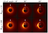 |
Fig. B.1. Time-averaged images of untilted and tilted disk models computed using H-AMR pipeline, for azimuthal viewing angle 0° and Rhigh = (1, 160). The white arrows indicate the projected direction of black hole spin, which is pointing away from Earth. The images are shown in linear scale. |
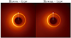 |
Fig. B.2. Time-averaged images of radiative models computed using koralpipelines. The images are shown in linear scale. |
Appendix C: Bayesian inference for combining multi-year results
Here we present the details of the multi-epoch scoring procedure.
C.1. Overview: a Bayesian view
We begin by making the following approximations and identifications:
 (C.1)
(C.1)
where D represents observed data, and (F, PA, M) respectively represents the total flux, the position angle of the black hole spin, and the mass of the source. In the above description, the subscript Yi denotes the value observed at different years.
Bayes theorem,
 (C.2)
(C.2)
here implies that
 (C.3)
(C.3)
We assume that the total flux is independent from year to year, and that the PA and mass are fixed. For two observations at different years, keeping these definitions for three sets of data: that in Y1, that in Y2, and that for the combined data set Y12, we note that if the data sets are independent as assumed throughout our analysis, then
 (C.4)
(C.4)
and therefore,
 (C.5)
(C.5)
Finally, we note that by definition,
 (C.6)
(C.6)
and therefore, we trivially have,
 (C.7)
(C.7)
This approach can be generalized for additional years of data by, e.g., adding more liklihood LYi and Bayesian evidence ZYi into the right hand sides of Eqs. (C.4) and (C.5).
C.2. Ensemble-based posterior construction
Within a given model, the posterior probability distribution on rotation (PA), and mass, is a natural output of any fitting procedure, such as the snapshot scoring applied in this paper. Typically, the posteriors of fitting individual snapshots to the EHT data do not overlap, with the intrinsic posterior widths being small in comparison to the distances between those from different snapshots. For the 2017 EHT observations we solved this with what we called “Ensemble-based Posterior Construction” (Appendix G of M87* 2017 VI, here EBPC). This is an example of Approximate Bayesian Computation (ABC) methods.
ABC is a method of posterior approximation in which forward modeled realizations of a random process are compared against data to generate a posterior on a subset of the model parameters. It is especially useful when the construction of realizations is expensive and the nature of the random process is not of intrinsic interest. In our case, the random process is the turbulence, and the model parameters of interest are the flux, PA, and mass. The procedure is to define a cut on a data/model statistic, here chosen to be χν2, keep fits that pass the cut, and use the resulting distribution of the parameters of interest. Demonstration that the resulting distributions faithfully capture truth values is presented in Appendices G.2 and G.3 of M87* 2017 VI, and used to generate parameter constraints in M87* 2017 V.
To produce ABC Posteriors (or EBPC posteriors) for a single simulation, the procedure is:
-
1.
Fit each snapshot to the data (N fits).
-
2.
Continuous posteriors are generated from kernal density estimations (KDEs) of the sampled values after applying desired χν2 cut.
Validation requires additional iterations using synthetic data sets drawn from simulation images. This procedure was already validated on the 2017 data.
Posteriors from the full set of models can be constructed by summing over posteriors from each model after selecting a model quality factor, e.g., AIS.
C.3. AIS – average image scoring
Average image scoring (AIS) is a procedure for assessing the likelihood that the data is drawn from the distribution of random processes associated with a given GRMHD simulation. This method is a modest extension of the standard χ2 test. What differs explicitly in this case is the probability distribution of the relevant fit statistic, i.e. the analog of the χ2-distribution, which is otherwise used to assess the test. This distinction is a consequence of the presence of stochastic, or “turbulent”, structures in the image that must be marginalized over. The primary complication is that these structures are neither sufficiently sampled in the GRMHD simulation image sets for a formal fitting process nor have a priori known statistics.
The solution is to assess a measure of the “distance” between the data and a fiducial image, here chosen to be the average image from a given simulation8 though such a choice is not unique, in light of the typical range of distances we expect based on the simulation itself. The distance measure we adopt is the reduced χ2, χν2, obtained by fitting the average image to the observational data. The value for the data is then evaluated against the value obtained by fitting the average image to synthetic data sets generated from individual snapshot images. A modest optimization is found by fitting the snapshot images to data generated from the average image, which is exactly equivalent in the absence of telescope gains due to the quadratic nature of the χν2 statistic, and is equivalent in practice in the presence of systematic uncertainties.
In principle, a Kolmogorov-Smirnov (KS) test may be used to formally assess probability that the data χν2 is drawn from the distribution of values from the simulation itself. In the past (M87* 2017 V) we have made the very conservative binary assessment of “inside” or “outside” the distribution, which for one value is equivalent. The outcome of AIS is a probability that the measured χν2 is drawn from the distribution.
C.4. Multi-epoch scoring
C.4.1. Statistical considerations
In principle, for each year Y and each simulation S, we will have a Bayesian evidence ZSY resulting from some overall fit quality assessment and a normalized posterior ℘SY(F, PA, M). The likelihood of a given parameter set is then given by
 (C.8)
(C.8)
from which we identify
 (C.9)
(C.9)
and
 (C.10)
The odds ratios between two simulations, S and S′, from a given year is simply
 (C.11)
The full parameter posterior in a given year is by Bayes theorem directly,
 (C.12)
where now the simulation-specific prior is the ZSY.
Because the measurements and the turbulent realizations are expected to be uncorrelated across years, combining multiple years is straightforward in principle. For a given simulation, the combined likelihood is
 (C.13)
This must be supplemented with (possibly joint) priors on FY1, FY2 (hereafter the joint prior is denoted as π). Under the assumption that total flux is independent from year to year, and that the PA is fixed (as is mass), π(FY1, FY2)=const and π(PAY1, PAY2)=δ(PAY1 − PAY2). We may then relate the posteriors and Bayesian evidence from the independent analyses on each year to those from the combined data set:
 (C.14)
and, again, from Bayes theorem directly,
 (C.15)
With the ZS for each model, we can construct the odds ratios immediately for model selection, and with the ℘S(FY1, FY2, PA, M) we can assess parameter constraints.
To implement the foregoing, we require estimates of the following functions:
-
ZSYi – The Bayesian evidence for a simulation in a given year Yi.
-
℘SYi}(FYi, PA,M) – The posterior probability distribution of the snapshot fit parameters in a given year Yi.
π(FY1,FY2) – The joint prior on the fluxes from year Y1 to year Y2, which we assume is constant, but really must merely be independent.
Now we turn to evaluation of these quantities.
C.4.2. Approximate integration
Given the natural expectations for the joint priors on flux, PA, and mass already described, we can combine the constraints from multiple years. Adopting AIS as the ZSY and the EBPC posterior as the ℘SY, the integrals in Eqs. C.14 and C.15 may be numerically performed explicitly.
Explicitly, upon choosing a flux prior that is completely uninformative, i.e., π(FY1, FY2)=1, and a fixed PA, i.e., π(PAY1, PAY2)=δ(PAY1 − PAY2), the updated Bayesian evidence for a single simulation obtained from combining the two years is
 (C.16)
and the posterior on PA and M is
 (C.17)
Combining multiple simulations gives
 (C.18)
This is attractive for a number of reasons. First, it is done as soon as scoring is finished. Second, the Bayesian odds ratios can place significantly improved cuts on the GRMHD library. For example, in our analysis, we compared normalized odd ratio for different models, and applied an arbitrary cut (see Fig. 7). Third, it has the virtue of being formally sensible.
The AIS score is not, however, exactly a Bayesian evidence, despite being used as such. In the absence of a full description of the turbulence and the capacity to effectively parameterize it and/or sample it, we do not have the capacity to generate true Bayesian evidences. However, generally, the AIS score is a more permissive, largely because we conservatively treat poorer-than-expected fits as acceptable. Nevertheless, there remains a possibility that a much better fit exists associated with a turbulent realization that was simply never sampled by the simulation. Similarly, the EBPC is not, exactly, a true posterior; it is typically broader. Again, this is unlikely to reject the true model since it serves to contaminate the acceptable parameter sets with formally bad fits.
Appendix D: AIS result summary
In Table D.1, we summarize the 2017 and 2018 AIS results for the fiducial models.
2017 and 2018 AIS results for the fiducial models
Appendix E: M/D distribution for exploratory, radiative models
Figure E.1 displays the posterior distributions of M/D for the radiative models fitted to 2017 (blue) and 2018 (red) datasets. The range of M/D is similar to some fiducial models shown in Fig. 4. As seen in most of the fiducuial models, snapshots fit to the 2018 data produce a distribution with a slightly higher peak than the 2017 data.
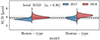 |
Fig. E.1. Violin plots of the M/D distributions from the snapshot scoring method against the 2017 and 2018 EHT observations, for the exploratory radiative models. |
All Tables
All Figures
|
Fig. 1. Representative reconstructed images and model images of M87∗. Left panels: EHT images of M87∗ from the 2018 (M87* 2018 I; Paper I of this series) and 2017 (M87* 2017 IV) campaigns. Middle panels: Example GRMHD model images drawn from the same model at two different times. Right panels: Theoretical images convolved with a 20 μas FWHM Gaussian beam. |
| In the text | |
|
Fig. 2. Poloidal (azimuthally averaged) and equatorial plane cuts of selected KHARMA GRMHD simulation snapshots of the two considered accretion modes, both with a* = +0.5. The MAD (left panels) and SANE (right panels) snapshots feature different ion temperatures (displayed in dimensionless units in the upper panels) and the plasma β parameter (displayed in the bottom panels), resulting in different emission properties. The solid black lines represent the σ = 1 surface. The high temperature near the polar axes is a consequence of conservative codes. The temperatures in the polar regions are considered unphysical and are masked out in the radiative transfer calculations (regions with σ > 1 or σ > 3). Here, rg ≡ GM/c2, the gravitational radius. |
| In the text | |
|
Fig. 3. Time-averaged images of all the fiducial models with Rlow = 1 and Rhigh = 40 in the image library. The white arrows indicate the projected direction of the black hole spin for the simulation geometry. The lower left corner is blank because there is no H-AMR SANE a* = −0.94 case in our model library. All images are shown in linear scale. |
| In the text | |
|
Fig. 4. Violin plots for M/D distributions from the snapshot scoring with 2017 and 2018 EHT observations for models with Rlow = 1 and Rhigh = 40 in the image library. The horizontal dashed black line and shaded gray region mark the ranges of M/D = 3.8 ± 0.4 μas reported in M87* 2017 I. |
| In the text | |
|
Fig. 5. Normalized distributions of the fitted position angle of the forward jet in selected fiducial thermal models based on the snapshot scoring with 2017 and 2018 observations, using the best-fit 10% of the images. The PA = 288° ±10° of the milliarcsecond-scale jet (Walker et al. 2018; Cui et al. 2023) is marked by the vertical dashed black line and shaded gray region. Left: Models with a black hole spin axis or a coordinate system axis (case a* = 0) pointing toward Earth. Prograde cases are shown in the top (a* > 0) and middle (a* = 0) panels, and the retrograde case (a* < 0) is shown in the bottom panel. Right: Models with a black hole spin axis or with a coordinate system axis (case a* = 0) pointing away from Earth. Prograde cases are shown in the top (a* > 0) and middle (for a* = 0 the matter angular momentum is always aligned with the coordinate axis) panels, and the retrograde case (a* < 0) is shown in the bottom panel. See text in this paper or Fig. 5 in M87* 2017 V for a description of the geometry of the black hole axis, flow rotational axis, and inclination angle. |
| In the text | |
|
Fig. 6. Demonstration of the multi-epoch scoring based on the KHARMA SANE model with (a*, Rlow, Rhigh)=(−0.5, 10, 160). The 2017 and 2018 snapshot scoring results for the given model are shown in the M/D – PA plane with the blue and red distributions, respectively. The larger the overlap between the red and blue distributions, the better the fit of the multi-epoch observations with a single model. The black profile indicates the normalized combined distribution of the best-fit parameters computed according to the multi-epoch scoring procedure (see Sect. 4.4 for details). The dashed lines and shaded areas are the same as explained in Figs. 4 and 5. |
| In the text | |
|
Fig. 7. Overview of the multi-epoch scoring results for all the fiducial models with black hole axes pointing away from Earth, and nonspinning black holes with a inclination angle i = 163°. The y-axis is the normalized odds ratio (see text for details), which indicates the relative preference by multi-epoch (2017 and 2018) observations. Models with different spins are shown in different panels. The green region marks passing models for which the relative odds ratio is ≥1%. Models with a relative odds ratio ≤0.001% are not shown. |
| In the text | |
|
Fig. 8. Time-averaged SEDs of selected best-bet models. The data points are taken from the multi-wavelength observations during the 2018 EHT campaign (EHT MWL Science Working Group 2024). The EHT observation is marked by the vertical red bar. The gray region of the SED indicates the variations of the SED for different snapshots. The colored histograms correspond to different radiative processes: synchrotron emission (blue), synchrotron photons scattered once (orange), synchrotron photons scattered twice (green), and bremsstrahlung (red). The total emission is displayed in black. |
| In the text | |
|
Fig. 9. Distribution of M/D obtained by fitting the 2017 (blue) and 2018 (red) data with the fiducial models shown in Table 3. These distributions are generated from the top 10% best-fitting snapshots by χ2. The results for models prepared by the KHARMA, H-AMR, and BHACpipelines are shown separately, together with the result for all the models combined. The distribution when combining both the 2017 and 2018 result by the multi-epoch scoring algorithm is shown as the black profile. The vertical dashed black line and shaded gray region mark the ranges of M/D = 3.8 ± 0.4 μas reported in Event Horizon Telescope Collaboration (2019a). |
| In the text | |
|
Fig. B.1. Time-averaged images of untilted and tilted disk models computed using H-AMR pipeline, for azimuthal viewing angle 0° and Rhigh = (1, 160). The white arrows indicate the projected direction of black hole spin, which is pointing away from Earth. The images are shown in linear scale. |
| In the text | |
|
Fig. B.2. Time-averaged images of radiative models computed using koralpipelines. The images are shown in linear scale. |
| In the text | |
|
Fig. E.1. Violin plots of the M/D distributions from the snapshot scoring method against the 2017 and 2018 EHT observations, for the exploratory radiative models. |
| In the text | |
Current usage metrics show cumulative count of Article Views (full-text article views including HTML views, PDF and ePub downloads, according to the available data) and Abstracts Views on Vision4Press platform.
Data correspond to usage on the plateform after 2015. The current usage metrics is available 48-96 hours after online publication and is updated daily on week days.
Initial download of the metrics may take a while.