© The Authors 2025

1. Introduction

The expansion rate of the Universe is one of the most fundamental physical parameters in astrophysics. The Hubble constant, H₀, describes the relative expansion rate of the Universe. H₀ has been measured so far with different methods, such as the cosmic microwave background (CMB) (e.g., Planck Collaboration VI 2020) and local distance ladders (e.g., Riess et al. 2022). However, there is a difference of 4 to 6σ between the two methods, namely the CMB and the local distance ladder (e.g. Verde et al. 2019; Di Valentino et al. 2021; Riess et al. 2021; Hu & Wang 2023). The recent estimate of H₀ from the CMB by the Planck Collaboration is 67.4 ± 0.5 km s⁻¹ Mpc⁻¹ (Planck Collaboration VI 2020), while the local distance ladder method by the Supernova H₀ for the Equation of State (SH0ES) team yielded H₀ = 73.0 ± 1.0 km s⁻¹ Mpc⁻¹ (Riess et al. 2022). One possible solution to the Hubble tension might be so-called early dark energy, which introduces an additional energy density to the early Universe (e.g., Hill & Baxter 2018), although the difference might be explained by observational systematics (e.g., Mörtsell et al. 2022).

Fast radio bursts (FRBs) are enigmatic coherent radio flashes that occur at cosmological distances (z ≳ 0.05; e.g., Lorimer et al. 2024; Bailes 2022; Petroff et al. 2019). They are characterized by a brief duration of approximately 1 ms and their exceptional brightness (e.g., Lorimer et al. 2007). The dispersion measure (DM) is a unique observable of FRBs. It represents a free electron density along the line of sight to an FRB. The definition of the DM is DM ≡∫n_eds, where n_e is the electron number density, and ds is the distance segment along the line of sight. The DM is proportional to the amount of plasma along a line of sight between an FRB source and an observer. Therefore, it can be used as an indicator of the redshift and distance to the FRB (Lorimer et al. 2007). The FRBs are critically important for addressing the issues of missing baryons (e.g., Macquart et al. 2020) and the equation of state of dark energy (e.g., Zhou et al. 2014). This made them a significant focus for further research. We rather focus on the Hubble tension in this particular paper because the existing difference between well-established methods (i.e., ∼10% systematics), including the CMB and the local distance ladder, underscores the importance of adding a new independent method to the comparison. The FRB method would be useful if it could achieve an accuracy better than ∼10% by mitigating the potential systematics in the method in the sense that it can distinguish between the H₀ values derived from the CMB and local distance ladder methods. Our primary focus is on leveraging the DM of FRBs as a unique distance indicator to derive H₀.

The observed DM (DM_obs) can be separated into three main components. One component is DM_MW, which is the DM contributed by Milky Way interstellar medium (ISM) and halo. Another is DM_h, which is the DM in a galaxy hosting one FRB source (FRB host galaxy). The other is DM_IGM, which is the DM in the intergalactic medium (IGM) between the Milky Way and a host galaxy,

$$\begin{array}{c}\hfill {\mathrm{DM}}_{\mathrm{obs}}={\mathrm{DM}}_{\mathrm{MW}}+{\mathrm{DM}}_{\mathrm{IGM}}+\frac{{\mathrm{DM}}_{\mathrm{h}}}{(1+z_{\mathrm{spec}})},\end{array}$$(1)

where z_spec is the spectroscopic redshift of the host galaxy. The DM_h is divided by 1 + z_spec to convert it into the observer’s frame, and the DM is given in units of pc cm⁻³. The DM_MW can be divided into two components, the disk and the halo (DM_MWdisk and DM_MWhalo, respectively),

$$\begin{array}{c}\hfill {\mathrm{DM}}_{\mathrm{MW}}={\mathrm{DM}}_{{\mathrm{MW}}_{\mathrm{disk}}}+{\mathrm{DM}}_{{\mathrm{MW}}_{\mathrm{halo}}}.\end{array}$$(2)

According to Eq. 9 in Zhou et al. (2014), the cosmic average of DM_IGM is proportional to H₀. The main focus of Zhou et al. (2014) was to discuss a constraint on the w parameter for the equation of state of dark energy with FRBs. In this work, we implement their formalization (their Eq. 9) in our analysis, combined with scattering, to measure H₀. Therefore, H₀ can be constrained with DM_IGM. To derive DM_IGM, DM_h has to be subtracted from DM_obs. However, in previous works (e.g., Hagstotz et al. 2022; Zhao et al. 2022), a certain distribution of DM_h was assumed for all FRB samples to calculate DM_IGM (see Sect. 6.2 for details). Therefore, there might be unknown systematic uncertainties in DM_h and DM_IGM in previous works.

The scattering time (τ) is the pulse-broadening effect of radio pulses, including pulsars and FRBs, due to the propagation through the plasma. The scattering time becomes longer when a radio pulse propagates in a larger amount of plasma with turbulence, and the scattering tail (Petroff et al. 2019) becomes more significant. The scattering time has a minimal impact on the pulse-broadening effect in the Milky May and IGM (e.g., Cordes et al. 2022). Therefore, we assumed that scattering only occurs within a host galaxy. The scattering time is a similar quantity as the DM_h in the sense that both increase with increasing amount of plasma in a host galaxy. Therefore, the scattering time has information on DM_h and is proportional to the square of DM_h (Cordes et al. 2022). The DM_h can be measured based on the observed scattering. This approach is free of the potential systematics involved in the assumption on DM_h, that is, either a fixed value of DM_h or a fixed shape of the distribution. This marks a novel application of the scattering time in determining DM_h, and it might improve the method employed to measure H₀. We focus on the capability of this approach using scattering to constrain H₀, while Cordes et al. (2022) used it to constrain the fraction of baryons in the IGM.

Throughout this paper, we assume the Planck 2018 results implemented in Astropy (Planck Collaboration VI 2020), that is, a Λ cold dark matter cosmology with (Ω_m, Ω_b) = (0.31, 0.049).

2. Method

We provide an overview of the method for constraining H₀ with DM and scattering. We followed the formalization presented in Cordes et al. (2022). Cordes et al. (2022) constrained the fraction of baryons in the intergalactic space with a given H₀. We instead focus on how accurately H₀ can be constrained under their formalization. The scattering time (τ) was used to measure a probability density function (PDF) of DM_h, where the PDF is described as a function of two parameters: DM_h and $A_{\tau }\stackrel{\sim }{F}G$. These two parameters are discussed in detail in Sect. 2.1. The integration of the PDF over all possible ranges of the two parameters (Cordes et al. 2022) was computed as a function of the redshift to derive the PDF of redshift. Using the 50th percentile of the PDF of the redshift, we can then determine a modeled redshift (z_model) that is derived by using DM and τ. z_model can be optimized to the observed redshift (z_spec) by changing H₀. The best-fit z_model provides us with the measurement of H₀.

2.1. Measuring DM_h

We adopted this equation to describe the rest-frame τ_rest as a function of DM_h,

$$\begin{array}{c}\hfill {\tau }_{\mathrm{rest}}({\mathrm{DM}}_{\mathrm{h}},v_{\mathrm{rest}})=C_{\tau }{v}_{\mathrm{rest}}^{-4}{A}_{\tau }\stackrel{\sim }{F}G{\left(\frac{{\mathrm{DM}}_{\mathrm{h}}}{100}\right)}^2,\end{array}$$(3)

where v_rest is the rest-frame frequency in units of GHz. The quantity C_τ = 0.48 ms (Cordes et al. 2022) is a numerical constant. To account for how empirical estimates for the scattering time are related to the e⁻¹ time, Cordes et al. (2022) introduced a dimensionless factor A_τ. $\stackrel{\sim }{F}$ (pc² km)^−1/3 is a parameter that characterizes density fluctuations. G is a dimensionless geometric factor. While the three parameters A_τ, $\stackrel{\sim }{F}$, and G have different physical meanings, they appear in the formalization as a product. Therefore, we treated the product $A_{\tau }\stackrel{\sim }{F}G$ as a single parameter. The prior assumption on the $A_{\tau }\stackrel{\sim }{F}G$ range is from 0.001 to 10 (pc² km)${}^{-\frac{1}{3}}$ (Cordes et al. 2022).

Two parameters, DM_h (pc cm⁻³) and $A_{\tau }\stackrel{\sim }{F}G$ (ϕ) ${({\mathrm{pc}}^2\mathrm{km})}^{-\frac{1}{3}}$, are used to describe the PDF of DM_h (Cordes et al. 2022):

$$\begin{array}{c}\hfill \begin{array}{cc}& f_{{\mathrm{DM}}_{\mathrm{h}},\varphi }({\mathrm{DM}}_{\mathrm{h}},\varphi |{\mathrm{DM}}_{\mathrm{obs}},z_{\mathrm{spec}},{\tau }_{\mathrm{obs}})\hfill \\ \hfill & \propto f_{{\mathrm{DM}}_{\mathrm{h}}}({\mathrm{DM}}_{\mathrm{h}}|{\mathrm{DM}}_{\mathrm{obs}},z_{\mathrm{spec}})\times f_{\tau }({\tau }_{\mathrm{obs}}-\widehat{\tau }).\hfill \end{array}\end{array}$$(4)

In Eq. (4), there are two terms on the right side: the first term uses DM, and the second term uses τ. The first term, f_DMh, is expressed as

$$\begin{array}{c}\hfill \begin{array}{cc}& f_{{\mathrm{DM}}_{\mathrm{h}}}({\mathrm{DM}}_{\mathrm{h}}|{\mathrm{DM}}_{\mathrm{obs}},{\mathrm{DM}}_{\mathrm{MW}},z_{\mathrm{spec}})\hfill \\ \hfill & =\frac{f_{{\mathrm{DM}}_{\mathrm{IGM}}}({\mathrm{DM}}_{\mathrm{IGM}}|{\mathrm{DM}}_{\mathrm{obs}},{\mathrm{DM}}_{\mathrm{MW}},z_{\mathrm{spec}})}{1+z_{\mathrm{spec}}}·\hfill \end{array}\end{array}$$(5)

f_DMh is determined using the PDF of DM_IGM (f_DMIGM), where DM${}_{\mathrm{IGM}}={\mathrm{DM}}_{\mathrm{obs}}-{\mathrm{DM}}_{{\mathrm{MW}}_{\mathrm{disk}}}-{\mathrm{DM}}_{{\mathrm{MW}}_{\mathrm{halo}}}-\frac{{\mathrm{DM}}_{\mathrm{h}}}{1+z_{\mathrm{spec}}}$. The uncertainty of DM_MW can be accounted for by introducing prior PDFs of DM_MWdisk and DM_MWhalo in Eq. (5). We assumed a flat PDF for DM_MWdisk centered at the mean value derived from the NE2001 (Cordes & Lazio 2002) with ±20% deviations (Cordes et al. 2022). A flat PDF of ${\mathrm{DM}}_{{\mathrm{MW}}_{\mathrm{halo}}}$ was assumed. It ranged from 25 to 80 pc cm⁻³ (Prochaska & Neeleman 2018; Shull & Danforth 2018; Prochaska & Zheng 2019; Yamasaki & Totani 2020). We used a log-normal distribution to characterize f_DMIGM (Cordes et al. 2022). The log-normal in the form, N(μ, σ), is a function of the following parameters:

$$\begin{array}{cc}\hfill \mu & =ln\left({\overline{\mathrm{DM}}}_{\mathrm{IGM}}\right)-\frac{{\sigma }^2}{2},\hfill \end{array}$$(6)

$$\begin{array}{cc}\hfill \sigma & =\sqrt{ln(1+{\left(\frac{{\sigma }_{{\mathrm{DM}}_{\mathrm{IGM}}}}{{\overline{\mathrm{DM}}}_{\mathrm{IGM}}}\right)}^2)},\hfill \end{array}$$(7)

with the cosmic variance of DM_IGM (σ_DMIGM). σ_DMIGM is described as follows:

$$\begin{array}{c}\hfill {\sigma }_{{\mathrm{DM}}_{\mathrm{IGM}}(z_{\mathrm{spec}})}=\sqrt{{\overline{\mathrm{DM}}}_{\mathrm{IGM}}(z_{\mathrm{spec}}){\mathrm{DM}}_{\mathrm{c}}},\end{array}$$(8)

where DM_c is a constant, that is, DM_c = 50 pc cm⁻³ (McQuinn 2014), and ${\overline{\mathrm{DM}}}_{\mathrm{IGM}}$ is the cosmic average of DM in the nonuniform intergalactic medium. The ${\overline{\mathrm{DM}}}_{\mathrm{IGM}}$ is described as follows:

$$\begin{array}{c}\hfill \begin{array}{cc}& {\overline{\mathrm{DM}}}_{\mathrm{IGM}}\hfill \\ \hfill & ={\mathrm{H}}_0\times f_{\mathrm{IGM}}\frac{3{\mathrm{\Omega }}_{b}c(Y_H+\frac{1}{2}{Y}_p)}{8\pi G{m}_p}{\displaystyle {\int }_0^z}\frac{1+z_{\mathrm{spec}}}{{\mathrm{\Omega }}_m{(1+z_{\mathrm{spec}})}^3+1-{\mathrm{\Omega }}_m}dz\hfill \end{array}\end{array}$$(9)

for a flat ΛCDM Universe. The proton mass is m_p = 1.67 × 10⁻²⁷ kg, and $Y_H=\frac{3}{4}$ and $Y_p=\frac{1}{4}$ are the mass fractions of hydrogen and helium, respectively (Zhou et al. 2014). The fraction of baryons in the IGM is f_IGM = 0.85 ± 0.05 (Cordes et al. 2022). The matter and baryon density are Ω_m and Ω_b (Zhou et al. 2014), respectively. For the cosmological parameters, we used the Planck 2018 results implemented in Astropy (Planck Collaboration VI 2020).

In the second term of Eq. (4), f_τ is the PDF of ${\tau }_{\mathrm{obs}}-\widehat{\tau }$, where τ_obs is the observed scattering, and $\widehat{\tau }$ is the theoretical value of the scattering. $\widehat{\tau }$ is described as follows:

$$\begin{array}{c}\hfill \widehat{\tau }=C_{\tau }{v}_{\mathrm{obs}}^{-4}\varphi {\left(\frac{{\mathrm{DM}}_{\mathrm{h}}}{100}\right)}^2{(1+z_{\mathrm{spec}})}^{-3},\end{array}$$(10)

where C_τ = 0.48 ms (Cordes et al. 2022). The observed frequency v_obs is given in units of GHz, and ϕ is the $A_{\tau }\stackrel{\sim }{F}G$ parameter (Cordes et al. 2022).

A Gaussian function was assumed to express $f_{\tau }({\tau }_{\mathrm{obs}}-\widehat{\tau })$ (Fig. 1 top). In the Gaussian function, the mean value was 0, and the observed error in the scattering (σ_τ) was adopted as the standard deviation. However, some FRBs only have upper limits of the scattering. In these cases, we assumed a flat PDF of ${\tau }_{\mathrm{obs}}-\widehat{\tau }$ (Fig. 1 bottom). We adopted 3σ_τ as the upper bound of the flat PDF.

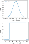Fig. 1. PDF of ${\tau }_{\mathrm{obs}}-\widehat{\tau }$. Top panel: Case for FRB 20220509G as an example (see Sect. 4 for details), assuming log $(A_{\tau }\stackrel{\sim }{F}G)=-1$. The peak of the PDF is at ${\tau }_{\mathrm{obs}}-\widehat{\tau }=0$, and the standard deviation is στ = 0.02 ms (see also Table 1). Bottom panel: FRBs with an upper limit of the scattering were given a flat PDF. We take FRB 20121102A as an example with the observed scattering of τobs < 9.6 ms (Sect. 4 and Table 1), assuming log $(A_{\tau }\stackrel{\sim }{F}G)=-1$. When $\widehat{\tau }$ is lower than 0 or greater than τobs, the probability is 0. When $\widehat{\tau }$ falls between 0 and τobs, the probability is nonzero and flat. We note that the vertical axes in both panels indicate relative quantities of the probability density.

To visualize Eq. (4), we show the PDF of DM_h as a function of DM_h and $A_{\tau }\stackrel{\sim }{F}G$ in the top panels of Fig. 2, where H₀ = 74.3 km s⁻¹ Mpc⁻¹ was assumed. By integrating $A_{\tau }\stackrel{\sim }{F}G$ from 0.001 to 10 ${({\mathrm{pc}}^2\mathrm{km})}^{-\frac{1}{3}}$, we present the PDF of DM_hin the bottom panels of Fig. 2.

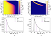Fig. 2. Two examples of the PDF in our observational samples. Top left panel: Three-dimensional image of fDMh for FRB 20181112A (see Sect. 4 and Table 1 for details). The x-axis is the DMh parameter from 20 to 600 pc cm−3. The y-axis is the $A_{\tau }\stackrel{\sim }{F}G$ parameter from −3 to 1 ${({\mathrm{pc}}^2\mathrm{km})}^{-\frac{1}{3}}$ in log scale. For a given DMh and $A_{\tau }\stackrel{\sim }{F}G$, the corresponding probability density in the log scale is presented by color. Bottom left panel: Integration of the PDF over the $A_{\tau }\stackrel{\sim }{F}G$ parameter from 0.001 to 10 ${({\mathrm{pc}}^2\mathrm{km})}^{-\frac{1}{3}}$, which provides us with the PDF of DMh. The purple line shows the 50 percentile of the PDF. The dashed black lines correspond to the 84.2 and 15.8 percentiles of the PDF (±σ). The 50 percentile is DMh = 85.6 pc cm−3, +σ = 78 pc cm−3, and −σ = 45.4 pc cm−3. Top right panel: Example of a 3D image of fDMh by using FRB 20191001A (see Sect. 4 and Table 1 for details). Bottom left panel: Same as the bottom left panel, but using FRB 20191001A. The 50 percentile is DMh = 143.3 pc cm−3, +σ = 89.3 pc cm−3, and −σ = 44.2 pc cm−3.

2.2. Redshift PDF

We used the following equation to calculate the redshift PDF (f_z) with the parameters of DM_obs and τ_obs:

$$\begin{array}{c}\hfill \begin{array}{cc}& f_z(z|{\mathrm{DM}}_{\mathrm{obs}},{\tau }_{\mathrm{obs}})\hfill \\ \hfill & \propto {\displaystyle \int \int d}{\mathrm{DM}}_{\mathrm{h}}d\varphi f_{{\mathrm{DM}}_{\mathrm{h}},\varphi }({\mathrm{DM}}_{\mathrm{h}},\varphi )\times f_{\tau }({\tau }_{\mathrm{obs}}-\widehat{\tau }),\hfill \end{array}\end{array}$$(11)

where the integration range of DM_h was [20, 1600] pc cm⁻³ (Cordes et al. 2022). In Eq. (11), we calculate the integration of all possible DM_h and $A_{\tau }\stackrel{\sim }{F}G$, which provided us with f_z.

To demonstrate f_z, we show examples of nine FRBs assuming H₀ = 74.3 km s⁻¹ Mpc⁻¹ in Fig. 3. Following Cordes et al. (2022), we present two prior assumptions on the $A_{\tau }\stackrel{\sim }{F}G$ range in this work: narrow [0.5, 2] and wide [0.001, 10] ${({\mathrm{pc}}^2\mathrm{km})}^{-\frac{1}{3}}$. The possible impact on the H₀ measurement with different prior assumptions on the $A_{\tau }\stackrel{\sim }{F}G$ parameter is discussed in Sects. 3 and 5. Throughout the paper, we present the results assuming the wide range of $A_{\tau }\stackrel{\sim }{F}G=[0.001,10]$${({\mathrm{pc}}^2\mathrm{km})}^{-\frac{1}{3}}$ as a fiducial model unless otherwise mentioned.

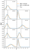Fig. 3. Nine examples representing the PDFs of redshift (z). These were randomly selected from our FRB samples (see Sect. 4 and Table 1 for details). H0 = 74.3 km s−1 Mpc−1 and DMh = [20, 1600] pc cm−3 were adopted. In each panel, we present PDFs based on two different ranges of $A_{\tau }\stackrel{\sim }{F}G$: [0.5, 2] (orange line) and [0.001, 10] (blue line) ${({\mathrm{pc}}^2\mathrm{km})}^{-\frac{1}{3}}$. The vertical dashed black line shows the observed redshift (zspec) in each panel.

2.3. Optimize H₀

We chose the 50 percentile of f_z to define the modeled redshift (z_model). By letting H₀ be a parameter (Eq. 9), z_model is a function of H₀. To optimize H₀, we compared z_model and z_spec, and we adjusted H₀ so that these two quantities became consistent within their errors, that is, z_model = z_spec. In Fig. 4, we show how z_model depends on H₀.

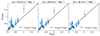Fig. 4. Observed redshift (zspec) vs. modeled redshift (zmodel) to optimize H0. To demonstrate how zmodel depends on H0, we present three values of H0, 60, 68, and 80 km s−1 Mpc−1, in the different panels. We used 30 FRBs (see Sect. 4 and Table 1 for details) with DMh = [20, 1600] pc cm−3 and $A_{\tau }\stackrel{\sim }{F}G=[0.001,10]$${({\mathrm{pc}}^2\mathrm{km})}^{-\frac{1}{3}}$. The black line corresponds to zmodel = zspec.

We only changed H₀ in Fig. 4 to demonstrate how this method works using 30 FRB samples (see Sect. 4 and Table 1 for details). However, H₀ degenerates with f_IGM in Eq. (9) because the observational error of f_IGM is ∼6% (e.g., Li et al. 2019; Cordes et al. 2022). Therefore, we present two cases of (i) f_IGM × H₀ as a single parameter in Eq. (9) and (ii) H₀ alone for a given f_IGM and its error in Sect. 5.

3. Simulation using mock FRB samples

3.1. Our method using scattering

Before we applied our method to the observed data, we demonstrate how accurate our measurements are compared with a previous method via simulations. Our aim is a prediction based on a reasonable sample size that can be achieved in the near future. With future instruments such as the CHIME Outrigger (Mena-Parra et al. 2022) and BURSTT (Lin et al. 2022; Ho et al. 2023), it would be feasible to identify 100 FRB host galaxies. Moreover, James et al. (2022) predicted that a sample of approximately 100 FRBs with spectroscopic redshifts would be sufficient to distinguish the ∼10% systematic discrepancies of the Hubble tension between the distance ladder and CMB methods. Therefore, we followed James et al. (2022) to decide the sample size of the mock data. We generated 100 mock FRBs as follows. First, we randomly selected redshift values for 100 mock FRBs from the CHIME FRB catalog (CHIME/FRB Collaboration 2021) based on the DM-derived redshift in Hashimoto et al. (2022) to create mock redshifts, z_mock. Then, we randomly sampled NE2001 values for 100 FRBs from the same catalog to create mock DM_MWdisk values (DM_{MWdisk, mock}). The adopted value of the mock DM_MWhalo (DM_{MWhalo, mock}) is 52.5 pc cm⁻³. Using z_mock, we calculated DM_IGM based on Eq. (9) assuming H₀ = 68 km s⁻¹ Mpc⁻¹ and f_IGM = 0.85, where the line-of-sight fluctuation of DM_IGM was taken into account based on Eq. (8) to create mock DM_IGM values (DM_IGM, mock). Figure 5 illustrates the generation of 100 DM_IGM, mock.

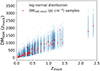Fig. 5. DMIGM, mock as a function of zmock. The red dots represent DMIGM, mock generated by using Eq. (8) at each zmock, taking the line-of-sight fluctuation of DMIGM into account. For a given zmock, we randomly selected one mock data point (red dot) from the blue dots. We iterated this process 100 times at the different zmock, generating 100 mock FRB data.

In general, DM_h is highly uncertain because DM_obs is an integrated quantity along a line of sight to an FRB, and hence, it is hard to separate between DM_h and DM_IGM without using scattering. For instance, Macquart et al. (2020) assumed DM_h = 50 pc cm⁻³ in their analysis. In contrast, Rafiei-Ravandi et al. (2021) conducted a cross-correlation analysis between CHIME FRB samples and galaxy catalogs to conclude that DM_h is about 400 pc cm⁻³, statistically. An even larger average DM_h might be suggested by a population-model approach (e.g., Wang & van Leeuwen 2024). These works highlight the significant uncertainty of the typical value of DM_h, ranging from ∼50 to ∼400 pc cm⁻³. To generate mock FRBs, we assumed a normal distribution with a mean of 200 pc cm⁻³ and a standard deviation of 50 pc cm⁻³ to create mock DM_h values (DM_h, mock).

Subsequently, using Eq. (1), we derived 100 mock DM_obs values (DM_obs, mock) from the z_mock, DM_IGM, mock, DM_MW, mock, and DM_h, mock. The mock scattering times (τ_mock) at the host frame 1 GHz for the 100 mock FRBs were determined using DM_h, mock with $A_{\tau }\stackrel{\sim }{F}G=$ 1 ${({\mathrm{pc}}^2\mathrm{km})}^{-\frac{1}{3}}$ and v = 1 GHz from Eq. (3). τ_mock at the observer’s frame (τ_mock, obs) was calculated by dividing τ_mock by a (1 + z_mock)³ factor, assuming ν⁻⁴ dependence of τ and a time-dilation factor of (1 + z). The mock error in scattering (σ_τ,mock) was simulated based on the median value of the fractional errors of τ_obs in Table 1 (i.e., σ_τ,mock = 5.2%). In summary, we generated 100 mock FRBs including z_mock, DM_IGM, mock, DM_MW, mock, DM_h, mock, DM_obs, mock, τ_mock, obs, and σ_τ,mock.

Figure 6 displays the PDF of H₀ × f_IGM and H₀ derived by applying our method to the 100 mock FRBs. The result is H${}_0\times f_{\mathrm{IGM}}=61.6_{-2.0}^{+1.6}$ km s⁻¹ Mpc⁻¹. This value corresponds to H${}_0=72.5_{-4.9}^{+4.7}$ km s⁻¹ Mpc⁻¹, where we assumed f_IGM = 0.85 taking the ±0.05 error of f_IGM (Cordes et al. 2022) into account. This reconstructed H₀ is consistent with the assumption made in the simulation, that is, H₀ = 68.0 km s⁻¹ Mpc⁻¹ within the statistical error.

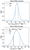Fig. 6. Simulation results using our method with mock FRB samples. Top panel: PDF of H0 × fIGM derived by using the 100 mock FRBs and our method with scattering (blue curve). The vertical dashed blue lines correspond to 84.2 and 15.8 percentiles (±σ) of the PDF. Bottom panel: PDF of H0 by changing the scale from H0 × fIGM (top panel) to H0. To generate the mock data, we assumed H0 = 68.0 km s−1 Mpc−1, which is shown by the solid vertical black line. The vertical dashed blue lines are the positive and negative standard deviations of H0 after taking the fIGM error into account, where the fIGM error is ±0.05 (Cordes et al. 2022).

3.2. Prior assumptions on the $A_{\tau }\stackrel{\sim }{F}G$ range in our method

In Eq. (11), the prior assumption on the $A_{\tau }\stackrel{\sim }{F}G$ range needs to be specified. Following Cordes et al. (2022), we briefly present how the narrow and wide $A_{\tau }\stackrel{\sim }{F}G$ ranges affect the H₀ measurements based on the 100 FRB mock data. We applied the method described in Sect. 2 to the 100 mock data, assuming $A_{\tau }\stackrel{\sim }{F}G=$ [0.5, 2] and [0.001, 10] ${({\mathrm{pc}}^2\mathrm{km})}^{-\frac{1}{3}}$. For a given value of f_IGM = 0.85  ±  0.05, the derived H₀ are 70.6${}_{-4.8}^{+4.4}$ and 72.5${}_{-4.9}^{+4.7}$ km s⁻¹ Mpc⁻¹ for $A_{\tau }\stackrel{\sim }{F}G=$ [0.5, 2] and [0.001, 10] ${({\mathrm{pc}}^2\mathrm{km})}^{-\frac{1}{3}}$, respectively. These reconstructed H₀ values are consistent with the assumption on H₀ = 68 km s⁻¹ Mpc⁻¹ within the errors. This is probably because $A_{\tau }\stackrel{\sim }{F}G=$ 1 ${({\mathrm{pc}}^2\mathrm{km})}^{-\frac{1}{3}}$ was adopted when the mock FRBs were generated (Sect. 3.1), and the two $A_{\tau }\stackrel{\sim }{F}G$ ranges cover this initial assumption reasonably well. Therefore, in this ideal case, no significant systematics due to the prior $A_{\tau }\stackrel{\sim }{F}G$ assumption are expected. However, this might not be the case when observed data are used to constrain H₀ because the physically reasonable range of $A_{\tau }\stackrel{\sim }{F}G$ is yet to be ascertained (Cordes et al. 2022). A further discussion of using observed data is described in Sect. 6.3.

3.3. Previous FRB method assuming DM_h

For a comparison, we tested a previous method without τ_mock, obs, assuming DM_h = 50 pc cm⁻³ to calculate DM_IGM. In this previous method, DM_IGM was calculated solely based on Eq. (1) for the same 100 FRB mock samples as were used for our method above. The top panel of Fig. 7 illustrates the resulting DM_IGM as a function of z_mock. We fit Eq. (9) to the mock data by changing H₀ as a fitting parameter. The derived PDFs of H₀ × f_IGM and H₀ are shown in the middle and bottom panels of Fig. 7, respectively. The result is H${}_0\times f_{\mathrm{IGM}}=66.9_{-2.8}^{+2.4}$ km s⁻¹ Mpc⁻¹. This value corresponds to H${}_0=78.7_{-5.7}^{+5.4}$ km s⁻¹ Mpc⁻¹, where we assumed f_IGM = 0.85 taking the ±0.05 error of f_IGM into account. This reconstructed H₀ significantly deviates from the assumed value of H₀ = 68.0 km s⁻¹ Mpc⁻¹ in the simulation.

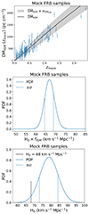Fig. 7. Simulation results using the previous method with mock FRB samples. Top panel: DMIGM, mock as a function of zmock. The blue dots with error bars show 100 mock FRB data, where DMIGM, mock is calculated by the previous method, assuming DMh = 50 pc cm−3. We fit Eq. (9) to the mock FRB data with a free parameter of H0. The best-fit function is shown by the solid black line, where H${}_0=78.7_{-5.7}^{+5.4}$ km s−1 Mpc−1. The gray shaded region indicates the line-of-sight fluctuation of DMIGM described by Eq. (8). Middle panel: Same as the top panel of Fig. 6, but using the previous method, assuming DMh = 50 pc cm−3. Bottom panel: Same as the bottom panel of Fig. 6, but using the previous method, assuming DMh = 50 pc cm−3.

3.4. Comparison between our method and the previous FRB method

Fig. 8 summarizes the systematic difference between the previous method and our method. In Fig. 8, we note that the reconstructed H₀ value with our method is consistent with the assumed value of H₀ = 68 km s⁻¹ Mpc⁻¹ within an uncertainty of 1σ. The 1σ error is presented by the dashed vertical orange lines in Fig. 8, where the assumed value (solid vertical black line) is within this error. Therefore, the reconstructed H₀ with our method does not deviate in a statistically significant way from the assumed value. The apparent offset between our method and the assumed value in Fig. 8 would be due to the statistical fluctuation owing to the random process in generating the mock FRB data. The systematic errors of H₀ are 15.7% and 6.6% for the previous method and our method, respectively. This corresponds to a reduction of the systematic error by 9.1%. By adopting our method, the statistical error slightly decreases from 3.9% to 2.9%, which corresponds to a reduction of 1%. This small reduction is probably due to a systematic effect, where the intrinsic variation in DM_h contaminates the DM_IGM variation in the previous method, while our method reduces this contamination by measuring the individual DM_h from scattering. Notably, the reduction in the systematic error is closely aligned with the systematics of the Hubble tension, that is, an ∼10% systematic uncertainty. This highlights the potential of our method to address the Hubble tension using forthcoming FRB datasets.

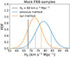Fig. 8. PDFs of H0 derived by our method (orange) with positive and negative standard deviations (orange vertical dashed lines) and the previous method (blue) with positive and negative standard deviations (vertical dashed blue lines), using the same 100 mock FRB data. The vertical black line indicates H0 = 68.0 km s−1 Mpc−1, which was assumed when we generated the 100 mock FRBs.

4. Selection criteria for the observed FRB samples

In the previous section, we applied our method to the simulated mock FRB samples to demonstrate how our method works compared with the previous method. In this section, we apply our method as described in Sect. 2 to 30 localized FRBs, which are shown in Table 1. In our method, we require localized FRBs with measurements of the spectroscopic redshift. Although more than 700 FRBs have been detected so far¹, only ∼40 of them are localized to host galaxies (e.g., Bhandari et al. 2022; Law et al. 2024). Additionally, our method requires information about the scattering time, which meant that we were left with 37 data sets to work with. According to Cordes et al. (2022), the reasonable range of the $A_{\tau }\stackrel{\sim }{F}G$ parameter is smaller than 10 ${({\mathrm{pc}}^2\mathrm{km})}^{-\frac{1}{3}}$. The PDF of the $A_{\tau }\stackrel{\sim }{F}G$ parameter can be computed by integrating Eq. (4) (the top panels of Fig. 2) over DM_h. We found that the PDFs of the $A_{\tau }\stackrel{\sim }{F}G$ parameter peak beyond 10 ${({\mathrm{pc}}^2\mathrm{km})}^{-\frac{1}{3}}$ for four FRB samples, that is, FRBs 20191228A, 20210405I, 20210410D, and 20220912A. Their PDFs of the $A_{\tau }\stackrel{\sim }{F}G$ parameter are mostly distributed at $A_{\tau }\stackrel{\sim }{F}G$ > 10 ${({\mathrm{pc}}^2\mathrm{km})}^{-\frac{1}{3}}$. The range of the peaks is $A_{\tau }\stackrel{\sim }{F}G=[10,1000]{({\mathrm{pc}}^2\mathrm{km})}^{-\frac{1}{3}}$ for these four samples. Therefore, we excluded these four FRBs from our samples as outliers in the $A_{\tau }\stackrel{\sim }{F}G$ parameter.

We also excluded three FRB samples that had negative DM_IGM as follows. The extragalactic component of the dispersion measure (DM_EG) is described as

$$\begin{array}{c}\hfill {\mathrm{DM}}_{\mathrm{EG}}\equiv {\mathrm{DM}}_{\mathrm{IGM}}+\frac{{\mathrm{DM}}_{\mathrm{h}}}{1+z_{\mathrm{spec}}}={\mathrm{DM}}_{\mathrm{obs}}-{\mathrm{DM}}_{{\mathrm{MW}}_{\mathrm{disk}}}-{\mathrm{DM}}_{{\mathrm{MW}}_{\mathrm{halo}}},\end{array}$$(12)

where DM_MWhalo = 52.5 pc cm⁻³, and DM_MWdisk was adopted from the NE2001 model. Here, certain values were used for DM_MWhalo and DM_MWdisk for the sample selection alone. The PDFs of DM_MWhalo and DM_MWdisk were taken into account in our method (Sect. 2) to constrain H₀. We found that DM_EG of FRB 20200120E and 20220319D are negative, indicating a negative DM_IGM. The DM_EG of FRB 20181030A is 9.93 pc cm⁻³. This value is lower than the lower bound of the prior assumption on DM_h ( = 20 pc cm⁻³) adopted in this work, following Cordes et al. (2022). These three FRBs correspond to negative DM_IGM. Therefore, we also excluded these three FRBs from our analysis. We excluded 7 of the 37 data sets, and the remaining 30 FRB samples were used in this work. Table 2 lists the 7 FRBs we excluded from our samples. In Fig. 9, we compare the scattering time at the rest-frame 1 GHz and DM_EG for the 30 FRB samples, along with 5 samples out of 7 excluded samples. We only show 5 excluded samples because 2 of the 7 have a negative DM_EG. These 5 excluded samples are close to or above the model line of $A_{\tau }\stackrel{\sim }{F}G=10{({\mathrm{pc}}^2\mathrm{km})}^{-\frac{1}{3}}$ (solid green line in Fig. 9). The empirical relation between the scattering at the rest-frame 1 GHz and DM_h expected from Galactic pulsar observations is described as

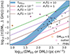Fig. 9. Scattering time vs. DMEG or DMh. The x-axis is the DMEG from Eq. (12) in the log scale for the FRB samples (black dots), and it shows DMh for the empirical relation based on Galactic pulsars (shaded blue region) and the $A_{\tau }\stackrel{\sim }{F}G$ models (solid colored lines). The y-axis is the scattering time at the rest-frame frequency of 1 GHz in the log scale. The black points are the 30 FRBs in our work. The pink circles are the $A_{\tau }\stackrel{\sim }{F}G$ outliers in our FRB samples. The orange circle is one of our FRB samples, which is DMIGM < 0 pc cm−3. The colored lines are the $A_{\tau }\stackrel{\sim }{F}G$ models from Eq. (3) with DMh = [20, 1600] pc cm−3. The blue area is the empirical relation derived from Galactic pulsars described in Eq. (13), which includes the geometrical scaling factor for the FRB samples.

$$\begin{array}{cc}& {log}_{10}({\tau }_{{\mathrm{MW}}_{\mathrm{psr}}})\hfill \\ \hfill & ={log}_{10}(1.9\times {10}^{-7}\mathrm{ms}{{\mathrm{DM}}_{\mathrm{h}}}^{1.5}\times (1+3.55\times {10}^5{{\mathrm{DM}}_{\mathrm{h}}}^3))\hfill \\ \hfill & +{log}_{10}(3)\pm 0.76,\hfill \end{array}$$(13)

(Cordes et al. 2022), which is shown as the shaded blue region in Fig. 9. The term of log₁₀(3) represents a scaling factor for taking the spherical wavefront difference between pulsars in the Milky Way and FRBs in host galaxies in the extragalactic Universe into account.

5. Results for the observed FRB samples

As described in Sect. 2.3, we treated f_IGM × H₀ as a single parameter to fit z_model to z_spec. The top panel of Fig. 10 shows the χ² of the fitting as a function of f_IGM × H₀,

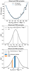Fig. 10. The results using our method with observed FRB samples. Top panel: χ2 described by Eq. (14) as a function of fIGM × H0 using the 30 FRB samples and our method. The black line indicates the χ2 values derived by changing fIGM × H0. The blue line is the best-fit polynomial function to χ2. Middle panel: PDF of fIGM × H0 from the χ2 (top panel). The vertical dashed black lines correspond to the 84.2 and 15.8 percentiles (±σ) of the PDF. Bottom panel: PDF of H0 by changing the scale from H0 × fIGM (middle panel) to H0 for a given fIGM = 0.85  ±  0.05. The solid vertical line indicates the peak of the PDF, and the dashed vertical lines indicate the uncertainty range of H0 after taking the 0.05 error of fIGM into account. The orange area indicates the CMB measurement of H0 (e.g., Planck Collaboration VI 2020). The blue area shows the measurement by local distance ladders (e.g., Riess et al. 2022).

$$\begin{array}{c}\hfill {\chi }^2={\displaystyle \sum _i}\frac{{(z_{\mathrm{model},\mathrm{i}}-z_{\mathrm{spec},\mathrm{i}})}^2}{{\sigma }_i^2},\end{array}$$(14)

where σ_i is the error of z_model of the ith FRB sample. We calculated the PDF of f_IGM × H₀ assuming PDF ∝exp(−χ²/2). The result is shown in the middle panel of Fig. 10 with prior assumptions on DM_h = [20, 1600] pc cm⁻³, and $A_{\tau }\stackrel{\sim }{F}G=[0.001,10]$${({\mathrm{pc}}^2\mathrm{km})}^{-\frac{1}{3}}$. The best-fit result is $f_{\mathrm{IGM}}\times {\mathrm{H}}_0=63.2_{-5.2}^{+4.8}$ km s⁻¹ Mpc⁻¹. Given f_IGM = 0.85  ± 0.05 (Cordes et al. 2022), the best-fit result corresponds to ${\mathrm{H}}_0=74.3_{-7.5}^{+7.2}$ km s⁻¹ Mpc⁻¹, where the uncertainty of f_IGM was taken into account (bottom panel of Fig. 10). The median value of DM_h in our analysis is DM_h$={103}_{-48}^{+68}$ pc cm⁻³ (see also Table 3 and Fig. 11). These errors were determined by calculating the median of the DM_h errors.

Fig. 11. Histogram of DMh derived by using scattering (see also Table 3).

6. Discussion

6.1. Comparison with the CMB and local distance ladders

Our measurement of the Hubble constant is H₀ = 74.3_−7.5^+7.2 km s⁻¹ Mpc⁻¹ using scattering. The central value of this measurement prefers the measurement from the local distance ladder (H₀ = 73.0 ± 1.0 km s⁻¹ Mpc⁻¹; Riess et al. 2022) than the CMB (H₀ = 67.7 ± 0.4 km s⁻¹ Mpc⁻¹; Planck Collaboration VI 2020). However, our measurement is still consistent with these two methods within the 1σ error. To address the Hubble tension with FRBs, both statistical and systematic errors have to be reduced in the future, as discussed in the following sections.

6.2. Comparison with the other FRB methods

Recently, some papers reported H₀ values that were constrained by FRBs, and the methods differed from ours. Hagstotz et al. (2022) assumed a normal distribution of DM_h with μ= 100 pc cm⁻³ and σ= 50 pc cm⁻³. They derived H₀ = 62.3 ± 9.1 km s⁻¹ Mpc⁻¹ using the DM_IGM–z relation with nine localized FRB samples. They assumed f_IGM = 0.84, where the difference from our assumption, f_IGM = 0.85, is negligibly small compared to the uncertainty of H₀. James et al. (2022) combined FRB population models and the DM_EG-z relation, which were parameterized by seven quantities for fitting, including μ and σ of the lognormal distribution of DM_h and H₀. They fit the model to the 76 FRB data obtained from The Commensal Real-time The Australian Square Kilometre Array Pathfinder Fast Transients Coherent (CRACO) survey (16 localized and 60 unlocalized), where the best-fit model indicates ${\mathrm{H}}_0={73}_{-8}^{+12}$ km s⁻¹ Mpc⁻¹, $\mu ={186}_{-48}^{+59}$ pc cm⁻³, and σ = 3.5 pc cm⁻³. They assumed f_IGM = 0.844. Zhao et al. (2022) used a Bayesian framework to estimate H${}_0=80.4_{-19.4}^{+24.1}$ km s⁻¹ Mpc⁻¹ with 12 unlocalized FRB samples with a prior assumption on a lognormal distribution of DM_h with μ = 68 pc cm⁻³ and σ = 0.88 pc cm⁻³. The samples were collected from FRBs detected with the Australian Square Kilometre Array Pathfinder (ASKAP). These previous works assumed a certain shape of the DM_h distribution, that is, a lognormal distribution or a normal distribution. Our method is free of this assumption. The scattering is used to derive the individual DM_h and DM_IGM in the samples.

Our result is ${\mathrm{H}}_0=74.3_{-7.5}^{+7.2}$ km s⁻¹ Mpc⁻¹ (Sect. 5), which is consistent with H₀ in these previous works within the statistical errors. In the previous method, however, there might be significant unknown systematics in the assumption on DM_h as we demonstrated in Sect. 3. Depending on the different assumptions on DM_h, the central values of derived H₀ systematically differ in the previous works mentioned above. This possible systematics is still smaller than the large statistical error based on the current FRB samples. However, the possible systematics would be problematic in the future when the statistical uncertainty is significantly reduced by large FRB samples. In contrast to previous studies, our method can minimize these systematics using the scattering time to derive the individual DM_h rather than assuming a certain DM_h distribution.

6.3. Prior assumption on the $A_{\tau }\stackrel{\sim }{F}G$ parameter range

Our simulation described in Sect. 3.2 suggests that the prior assumption on the $A_{\tau }\stackrel{\sim }{F}G$ range does not significantly impact the best-fit result of H₀, as far as the prior covers the true $A_{\tau }\stackrel{\sim }{F}G$ value. However, this might not be the case when observed data are used because the true $A_{\tau }\stackrel{\sim }{F}G$ distribution is unknown (Cordes et al. 2022).

We compared results based on the observed data, assuming narrow and wide ranges of $A_{\tau }\stackrel{\sim }{F}G=[0.5,2]$ and [0.001, 10] ${({\mathrm{pc}}^2\mathrm{km})}^{-\frac{1}{3}}$, respectively. Figure 12 shows a comparison between the narrow and wide ranges of $A_{\tau }\stackrel{\sim }{F}G$ in z_model versus z_spec. The figure includes our 30 FRB samples, where we fixed the value of f_IGM × H₀ = 63.2 km s⁻¹ Mpc⁻¹ to highlight the difference between the $A_{\tau }\stackrel{\sim }{F}G$ ranges. χ² is 75.1 for the narrow range, and 37.9 is for the wide range. We found that z_model with $A_{\tau }\stackrel{\sim }{F}G=[0.5,2]$${({\mathrm{pc}}^2\mathrm{km})}^{-\frac{1}{3}}$ are systematically lower than that with $A_{\tau }\stackrel{\sim }{F}G=[0.001,10]$${({\mathrm{pc}}^2\mathrm{km})}^{-\frac{1}{3}}$, indicating that the different prior assumptions on $A_{\tau }\stackrel{\sim }{F}G$ systematically affect the H₀ measurement. To demonstrate this point, we present the best-fit z_model to z_spec for two cases of the $A_{\tau }\stackrel{\sim }{F}G$ ranges by optimizing f_IGM × H₀ in the top panel of Fig. 13. The best-fit f_IGM × H₀ (and χ²) are $51.5_{-4.4}^{+4.4}$ km s⁻¹ Mpc⁻¹ (58) and $63.2_{-5.2}^{+4.8}$ km s⁻¹ Mpc⁻¹ (37.9) for the narrow and wide ranges, respectively (middle panel of Fig. 13). Given a fixed value of f_IGM = 0.85 ± 0.05, these correspond to ${\mathrm{H}}_0=60.6_{-6.3}^{+6.3}$ km s⁻¹ Mpc⁻¹ and ${\mathrm{H}}_0=74.3_{-7.5}^{+7.2}$ km s⁻¹ Mpc⁻¹ for the narrow and wide $A_{\tau }\stackrel{\sim }{F}G$ ranges, respectively (bottom panel of Fig. 13)

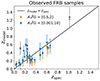Fig. 12. zmodel vs. zobs, comparing two prior assumptions on the $A_{\tau }\stackrel{\sim }{F}G$ ranges using the 30 FRB samples and our method. The blue points with error bars assume $A_{\tau }\stackrel{\sim }{F}G$ =[0.001, 10] ${({\mathrm{pc}}^2\mathrm{km})}^{-\frac{1}{3}}$. The orange points with error bars assume $A_{\tau }\stackrel{\sim }{F}G$ =[0.5, 2] ${({\mathrm{pc}}^2\mathrm{km})}^{-\frac{1}{3}}$. To demonstrate how the result depends on the prior assumption on the $A_{\tau }\stackrel{\sim }{F}G$ range, the identical value of fIGM × H0 = 63.2 km s−1 Mpc−1 is adopted for both cases.

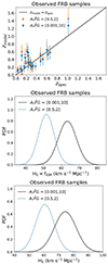Fig. 13. Comparison of results across different $A_{\tau }\stackrel{\sim }{F}G$ ranges. Top panel: zmodel vs. zobs, same as Fig. 12, but with optimized fIGM × H0 values, where fIGM × H0 are $51.5_{-4.4}^{+4.4}$ km s−1 Mpc−1 and $63.2_{-5.2}^{+4.8}$ km s−1 Mpc−1 for the narrow and wide $A_{\tau }\stackrel{\sim }{F}G$ ranges, respectively. Middle panel: PDF of fIGM × H0 using the 30 FRB samples and our method. The solid black line corresponds to the wide $A_{\tau }\stackrel{\sim }{F}G$ range, and the dashed blue line corresponds to the narrow $A_{\tau }\stackrel{\sim }{F}G$ range. Bottom panel: PDF of H0 for a given fIGM = 0.85 ± 0.05 using the 30 FRB samples and our method.

The χ² value is higher for the narrow $A_{\tau }\stackrel{\sim }{F}G$ range, suggesting a worse fit to the observed data with $A_{\tau }\stackrel{\sim }{F}G=[0.5,2]$${({\mathrm{pc}}^2\mathrm{km})}^{-\frac{1}{3}}$. This might suggest that the narrow range does not fully cover the true $A_{\tau }\stackrel{\sim }{F}G$ distribution in the FRB samples. The narrow-range model therefore does not fit the observed data well. In contrast, the wide $A_{\tau }\stackrel{\sim }{F}G$ range is expected to perform better because its coverage in the $A_{\tau }\stackrel{\sim }{F}G$ parameter space is better. We speculate that the wide $A_{\tau }\stackrel{\sim }{F}G$ range covers the true $A_{\tau }\stackrel{\sim }{F}G$ distribution better, and it would be closer to the ideal situation of our simulation without significant systematics (Sect. 3.2) than the narrow $A_{\tau }\stackrel{\sim }{F}G$ range. In this sense, the wide $A_{\tau }\stackrel{\sim }{F}G$ range would be preferable in our analysis.

Detailed investigations of the $A_{\tau }\stackrel{\sim }{F}G$ impact on f_igm × H₀ have to be made and the optimal range of $A_{\tau }\stackrel{\sim }{F}G$ must be determined before our method can address the Hubble tension properly. Physically motivated constraints of the $A_{\tau }\stackrel{\sim }{F}G$ parameter would also play an important role in searching for the optimal $A_{\tau }\stackrel{\sim }{F}G$ range. We leave these points as future work because we focused on proposing a method for constraining H₀ with the scattering rather than emphasizing the current accuracy in this paper.

6.4. Future FRB samples

Currently, the number of localized FRBs is limited to ∼40 (e.g., Bhandari et al. 2022; Law et al. 2024). About 100 localized FRBs would be sufficient to clarify the Hubble tension with an uncertainty of ∼2.5 km s⁻¹ Mpc⁻¹ (James et al. 2022). More FRBs will be localized with scattering measurements with future instruments, including the CHIME outrigger (Mena-Parra et al. 2022), the Deep Synoptic Array-110, ASKAP, and the Bustling Universe Radio Survey Telescope in Taiwan (BURSTT) (Lin et al. 2022; Ho et al. 2023). BURSTT can localize ∼100 FRBs per year (Lin et al. 2022) to identify host galaxies with scattering measurements. Unlocalized FRBs can be used to derive the redshift statistically to further increase the samples (e.g., Zhao et al. 2022). Therefore, our method can be tested with better statistics in the near future.

7. Conclusions

A significant difference of 4 to 6 sigma exists in determining the Hubble constant (H₀) for two distinct methods, the cosmic microwave background (CMB) and the local distance ladders. This difference is most likely caused by unknown systematic errors. Therefore, devising an independent method for measuring H₀ is the most important mission for addressing this unresolved puzzle. The FRBs offer a unique observable, DM_IGM, which is a new distance indicator to derive H₀. We summarize the result of this work below.

1. DM_h had to be assumed in previous works to derive DM_IGM. The scattering enabled us to measure DM_IGM with a parameter that combined a pulse profile, density fluctuations, and the geometry of a scattering screen ($A_{\tau }\stackrel{\sim }{F}G$ parameter). We used this parameterization for 30 FRBs with scattering measurements to model the redshifts, and we compared them with the observed redshifts (spectroscopic redshifts) to constrain H₀.

2. We demonstrated that our method reduces the systematic error of H₀ by 9.1% compared to the previous method, and the statistical error is reduced by 1%. The reduction in systematic error is comparable to the Hubble tension (∼10%), indicating that our method can address the Hubble tension using future FRB samples.

3. We measured a Hubble constant of H₀ = 74.3_−7.5^+7.2 km s⁻¹ Mpc⁻¹ with our method using scattering. The central value of this result prefers the measurement from the local distance ladder (H₀ = 73.0 ± 1.0 km s⁻¹ Mpc⁻¹; Riess et al. 2022) over the CMB (H₀ = 67.7 ± 0.4 km s⁻¹ Mpc⁻¹; Planck Collaboration VI 2020). However, our measurement is still consistent with the two methods within an error of 1σ.

We described two future directions to reduce the error in our measurement. The first direction is to use more localized FRBs with scattering measurements, which are to be detected with future instruments, including BURSTT (Lin et al. 2022). BURSTT is the Taiwanese radio array, which can localize ∼100 FRBs per year to identify host galaxies with scattering (Lin et al. 2022). The second direction is to statistically treat unlocalized FRBs to further increase the samples (e.g., Zhao et al. 2022).

Acknowledgments

We would like to express our deepest appreciation to the anonymous referee for the comprehensive and thoughtful review of our manuscript. Their detailed examination and insightful suggestions have played a crucial role in refining our work, and the constructive feedback has greatly enhanced the overall quality and clarity of the paper. T-CY is grateful to Ms. Poya Wang for insightful discussions. T-CY is also grateful to Dr. Shotaro Yamasaki for insightful discussions. TG acknowledges the support of the National Science and Technology Council of Taiwan through grants 108-2628-M-007-004-MY3, 111-2112-M-007-021, and 112-2123-M-001-004-. TH acknowledges the support of the National Science and Technology Council of Taiwan through grants 110-2112-M-005-013-MY3, 110-2112-M-007-034-, 113-2112-M-005-009-MY3, and 113-2123-M-001-008-. We acknowledge the use of the CHIME/FRB Public Database, provided at https://www.chime-frb.ca/ by the CHIME/FRB Collaboration. This research made use of Astropy, a community-developed core Python package for Astronomy (Astropy Collaboration 2018).

References

All Tables

All Figures

Fig. 1. PDF of ${\tau }_{\mathrm{obs}}-\widehat{\tau }$. Top panel: Case for FRB 20220509G as an example (see Sect. 4 for details), assuming log $(A_{\tau }\stackrel{\sim }{F}G)=-1$. The peak of the PDF is at ${\tau }_{\mathrm{obs}}-\widehat{\tau }=0$, and the standard deviation is στ = 0.02 ms (see also Table 1). Bottom panel: FRBs with an upper limit of the scattering were given a flat PDF. We take FRB 20121102A as an example with the observed scattering of τobs < 9.6 ms (Sect. 4 and Table 1), assuming log $(A_{\tau }\stackrel{\sim }{F}G)=-1$. When $\widehat{\tau }$ is lower than 0 or greater than τobs, the probability is 0. When $\widehat{\tau }$ falls between 0 and τobs, the probability is nonzero and flat. We note that the vertical axes in both panels indicate relative quantities of the probability density.

In the text

Fig. 2. Two examples of the PDF in our observational samples. Top left panel: Three-dimensional image of fDMh for FRB 20181112A (see Sect. 4 and Table 1 for details). The x-axis is the DMh parameter from 20 to 600 pc cm−3. The y-axis is the $A_{\tau }\stackrel{\sim }{F}G$ parameter from −3 to 1 ${({\mathrm{pc}}^2\mathrm{km})}^{-\frac{1}{3}}$ in log scale. For a given DMh and $A_{\tau }\stackrel{\sim }{F}G$, the corresponding probability density in the log scale is presented by color. Bottom left panel: Integration of the PDF over the $A_{\tau }\stackrel{\sim }{F}G$ parameter from 0.001 to 10 ${({\mathrm{pc}}^2\mathrm{km})}^{-\frac{1}{3}}$, which provides us with the PDF of DMh. The purple line shows the 50 percentile of the PDF. The dashed black lines correspond to the 84.2 and 15.8 percentiles of the PDF (±σ). The 50 percentile is DMh = 85.6 pc cm−3, +σ = 78 pc cm−3, and −σ = 45.4 pc cm−3. Top right panel: Example of a 3D image of fDMh by using FRB 20191001A (see Sect. 4 and Table 1 for details). Bottom left panel: Same as the bottom left panel, but using FRB 20191001A. The 50 percentile is DMh = 143.3 pc cm−3, +σ = 89.3 pc cm−3, and −σ = 44.2 pc cm−3.

In the text

Fig. 3. Nine examples representing the PDFs of redshift (z). These were randomly selected from our FRB samples (see Sect. 4 and Table 1 for details). H0 = 74.3 km s−1 Mpc−1 and DMh = [20, 1600] pc cm−3 were adopted. In each panel, we present PDFs based on two different ranges of $A_{\tau }\stackrel{\sim }{F}G$: [0.5, 2] (orange line) and [0.001, 10] (blue line) ${({\mathrm{pc}}^2\mathrm{km})}^{-\frac{1}{3}}$. The vertical dashed black line shows the observed redshift (zspec) in each panel.

In the text

Fig. 4. Observed redshift (zspec) vs. modeled redshift (zmodel) to optimize H0. To demonstrate how zmodel depends on H0, we present three values of H0, 60, 68, and 80 km s−1 Mpc−1, in the different panels. We used 30 FRBs (see Sect. 4 and Table 1 for details) with DMh = [20, 1600] pc cm−3 and $A_{\tau }\stackrel{\sim }{F}G=[0.001,10]$${({\mathrm{pc}}^2\mathrm{km})}^{-\frac{1}{3}}$. The black line corresponds to zmodel = zspec.

In the text

	Fig. 5. DMIGM, mock as a function of zmock. The red dots represent DMIGM, mock generated by using Eq. (8) at each zmock, taking the line-of-sight fluctuation of DMIGM into account. For a given zmock, we randomly selected one mock data point (red dot) from the blue dots. We iterated this process 100 times at the different zmock, generating 100 mock FRB data.
In the text

Fig. 6. Simulation results using our method with mock FRB samples. Top panel: PDF of H0 × fIGM derived by using the 100 mock FRBs and our method with scattering (blue curve). The vertical dashed blue lines correspond to 84.2 and 15.8 percentiles (±σ) of the PDF. Bottom panel: PDF of H0 by changing the scale from H0 × fIGM (top panel) to H0. To generate the mock data, we assumed H0 = 68.0 km s−1 Mpc−1, which is shown by the solid vertical black line. The vertical dashed blue lines are the positive and negative standard deviations of H0 after taking the fIGM error into account, where the fIGM error is ±0.05 (Cordes et al. 2022).

In the text

Fig. 7. Simulation results using the previous method with mock FRB samples. Top panel: DMIGM, mock as a function of zmock. The blue dots with error bars show 100 mock FRB data, where DMIGM, mock is calculated by the previous method, assuming DMh = 50 pc cm−3. We fit Eq. (9) to the mock FRB data with a free parameter of H0. The best-fit function is shown by the solid black line, where H${}_0=78.7_{-5.7}^{+5.4}$ km s−1 Mpc−1. The gray shaded region indicates the line-of-sight fluctuation of DMIGM described by Eq. (8). Middle panel: Same as the top panel of Fig. 6, but using the previous method, assuming DMh = 50 pc cm−3. Bottom panel: Same as the bottom panel of Fig. 6, but using the previous method, assuming DMh = 50 pc cm−3.

In the text

	Fig. 8. PDFs of H0 derived by our method (orange) with positive and negative standard deviations (orange vertical dashed lines) and the previous method (blue) with positive and negative standard deviations (vertical dashed blue lines), using the same 100 mock FRB data. The vertical black line indicates H0 = 68.0 km s−1 Mpc−1, which was assumed when we generated the 100 mock FRBs.
In the text

Fig. 9. Scattering time vs. DMEG or DMh. The x-axis is the DMEG from Eq. (12) in the log scale for the FRB samples (black dots), and it shows DMh for the empirical relation based on Galactic pulsars (shaded blue region) and the $A_{\tau }\stackrel{\sim }{F}G$ models (solid colored lines). The y-axis is the scattering time at the rest-frame frequency of 1 GHz in the log scale. The black points are the 30 FRBs in our work. The pink circles are the $A_{\tau }\stackrel{\sim }{F}G$ outliers in our FRB samples. The orange circle is one of our FRB samples, which is DMIGM < 0 pc cm−3. The colored lines are the $A_{\tau }\stackrel{\sim }{F}G$ models from Eq. (3) with DMh = [20, 1600] pc cm−3. The blue area is the empirical relation derived from Galactic pulsars described in Eq. (13), which includes the geometrical scaling factor for the FRB samples.

In the text

Fig. 10. The results using our method with observed FRB samples. Top panel: χ2 described by Eq. (14) as a function of fIGM × H0 using the 30 FRB samples and our method. The black line indicates the χ2 values derived by changing fIGM × H0. The blue line is the best-fit polynomial function to χ2. Middle panel: PDF of fIGM × H0 from the χ2 (top panel). The vertical dashed black lines correspond to the 84.2 and 15.8 percentiles (±σ) of the PDF. Bottom panel: PDF of H0 by changing the scale from H0 × fIGM (middle panel) to H0 for a given fIGM = 0.85  ±  0.05. The solid vertical line indicates the peak of the PDF, and the dashed vertical lines indicate the uncertainty range of H0 after taking the 0.05 error of fIGM into account. The orange area indicates the CMB measurement of H0 (e.g., Planck Collaboration VI 2020). The blue area shows the measurement by local distance ladders (e.g., Riess et al. 2022).

In the text

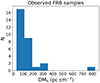	Fig. 11. Histogram of DMh derived by using scattering (see also Table 3).
In the text

Fig. 12. zmodel vs. zobs, comparing two prior assumptions on the $A_{\tau }\stackrel{\sim }{F}G$ ranges using the 30 FRB samples and our method. The blue points with error bars assume $A_{\tau }\stackrel{\sim }{F}G$ =[0.001, 10] ${({\mathrm{pc}}^2\mathrm{km})}^{-\frac{1}{3}}$. The orange points with error bars assume $A_{\tau }\stackrel{\sim }{F}G$ =[0.5, 2] ${({\mathrm{pc}}^2\mathrm{km})}^{-\frac{1}{3}}$. To demonstrate how the result depends on the prior assumption on the $A_{\tau }\stackrel{\sim }{F}G$ range, the identical value of fIGM × H0 = 63.2 km s−1 Mpc−1 is adopted for both cases.

In the text

Fig. 13. Comparison of results across different $A_{\tau }\stackrel{\sim }{F}G$ ranges. Top panel: zmodel vs. zobs, same as Fig. 12, but with optimized fIGM × H0 values, where fIGM × H0 are $51.5_{-4.4}^{+4.4}$ km s−1 Mpc−1 and $63.2_{-5.2}^{+4.8}$ km s−1 Mpc−1 for the narrow and wide $A_{\tau }\stackrel{\sim }{F}G$ ranges, respectively. Middle panel: PDF of fIGM × H0 using the 30 FRB samples and our method. The solid black line corresponds to the wide $A_{\tau }\stackrel{\sim }{F}G$ range, and the dashed blue line corresponds to the narrow $A_{\tau }\stackrel{\sim }{F}G$ range. Bottom panel: PDF of H0 for a given fIGM = 0.85 ± 0.05 using the 30 FRB samples and our method.

In the text

References

- Astropy Collaboration (Price-Whelan, A. M., et al.) 2018, AJ, 156, 123 [Google Scholar]
- Bailes, M. 2022, Science, 378, abj3043 [NASA ADS] [CrossRef] [Google Scholar]
- Bannister, K. W., Deller, A. T., Phillips, C., et al. 2019, Science, 365, 565 [NASA ADS] [CrossRef] [Google Scholar]
- Bhandari, S., Kumar, P., Shannon, R. M., & Macquart, J. P. 2019, ATel, 12940, 1 [NASA ADS] [Google Scholar]
- Bhandari, S., Bannister, K. W., Lenc, E., et al. 2020, ApJ, 901, L20 [NASA ADS] [CrossRef] [Google Scholar]
- Bhandari, S., Heintz, K. E., Aggarwal, K., et al. 2022, AJ, 163, 69 [NASA ADS] [CrossRef] [Google Scholar]
- Bhandari, S., Gordon, A. C., Scott, D. R., et al. 2023, ApJ, 948, 67 [NASA ADS] [CrossRef] [Google Scholar]
- Caleb, M., Driessen, L. N., Gordon, A. C., et al. 2023, MNRAS, 524, 2064 [NASA ADS] [CrossRef] [Google Scholar]
- Cassanelli, T., Leung, C., Sanghavi, P., et al. 2023, ArXiv e-prints [arXiv:2307.09502] [Google Scholar]
- Chawla, P., Andersen, B. C., Bhardwaj, M., et al. 2020, ApJ, 896, L41 [NASA ADS] [CrossRef] [Google Scholar]
- CHIME/FRB Collaboration (Andersen, B. C., et al.) 2019, ApJ, 885, L24 [Google Scholar]
- CHIME/FRB Collaboration (Amiri, M., et al.) 2021, ApJS, 257, 59 [NASA ADS] [CrossRef] [Google Scholar]
- Cho, H., Macquart, J.-P., Shannon, R. M., et al. 2020, ApJ, 891, L38 [NASA ADS] [CrossRef] [Google Scholar]
- Connor, L., Ravi, V., Catha, M., et al. 2023, ApJ, 949, L26 [NASA ADS] [CrossRef] [Google Scholar]
- Cordes, J. M., & Lazio, T. J. W. 2002, ArXiv e-prints [arXiv:astro-ph/0207156] [Google Scholar]
- Cordes, J. M., Ocker, S. K., & Chatterjee, S. 2022, ApJ, 931, 88 [NASA ADS] [CrossRef] [Google Scholar]
- Day, C. K., Deller, A. T., Shannon, R. M., et al. 2020, MNRAS, 497, 3335 [NASA ADS] [CrossRef] [Google Scholar]
- Di Valentino, E., Mena, O., Pan, S., et al. 2021, Class. Quant. Grav., 38, 153001 [NASA ADS] [CrossRef] [Google Scholar]
- Driessen, L. N., Barr, E. D., Buckley, D. A. H., et al. 2024, MNRAS, 527, 3659 [Google Scholar]
- Hagstotz, S., Reischke, R., & Lilow, R. 2022, MNRAS, 511, 662 [CrossRef] [Google Scholar]
- Hashimoto, T., Goto, T., Chen, B. H., et al. 2022, MNRAS, 511, 1961 [NASA ADS] [CrossRef] [Google Scholar]
- Hill, J. C., & Baxter, E. J. 2018, JCAP, 2018, 037 [CrossRef] [Google Scholar]
- Ho, S. C. C., Hashimoto, T., Goto, T., et al. 2023, ApJ, 950, 53 [NASA ADS] [CrossRef] [Google Scholar]
- Hu, J.-P., & Wang, F.-Y. 2023, Universe, 9, 94 [CrossRef] [Google Scholar]
- James, C. W., Ghosh, E. M., Prochaska, J. X., et al. 2022, MNRAS, 516, 4862 [NASA ADS] [CrossRef] [Google Scholar]
- Josephy, A., Chawla, P., Fonseca, E., et al. 2019, ApJ, 882, L18 [NASA ADS] [CrossRef] [Google Scholar]
- Kumar, P., Day, C. K., Shannon, R. M., et al. 2020, ATel, 13694, 1 [NASA ADS] [Google Scholar]
- Kumar, P., Shannon, R. M., Moss, V., Qiu, H., & Bhandari, S. 2021, ATel, 14502, 1 [NASA ADS] [Google Scholar]
- Law, C. J., Butler, B. J., Prochaska, J. X., et al. 2020, ApJ, 899, 161 [NASA ADS] [CrossRef] [Google Scholar]
- Law, C. J., Sharma, K., Ravi, V., et al. 2024, ApJ, 967, 29 [NASA ADS] [CrossRef] [Google Scholar]
- Lee, K.-G., Khrykin, I. S., Simha, S., et al. 2023, ApJ, 954, L7 [NASA ADS] [CrossRef] [Google Scholar]
- Li, Z., Gao, H., Wei, J.-J., et al. 2019, ApJ, 876, 146 [NASA ADS] [CrossRef] [Google Scholar]
- Lin, H. H., Lin, K. Y., Li, C. T., et al. 2022, PASP, 134, 094106 [NASA ADS] [CrossRef] [Google Scholar]
- Lorimer, D. R., Bailes, M., McLaughlin, M. A., Narkevic, D. J., & Crawford, F. 2007, Science, 318, 777 [Google Scholar]
- Lorimer, D. R., McLaughlin, M. A., & Bailes, M. 2024, Ap&SS, 369, 59 [NASA ADS] [CrossRef] [Google Scholar]
- Macquart, J.-P., Prochaska, J. X., McQuinn, M., et al. 2020, Nature, 581, 391 [Google Scholar]
- McQuinn, M. 2014, ApJ, 780, L33 [Google Scholar]
- Mena-Parra, J., Leung, C., Cary, S., et al. 2022, AJ, 163, 48 [NASA ADS] [CrossRef] [Google Scholar]
- Mörtsell, E., Goobar, A., Johansson, J., & Dhawan, S. 2022, ApJ, 935, 58 [CrossRef] [Google Scholar]
- Nimmo, K., Hessels, J. W. T., Kirsten, F., et al. 2022, Nat. Astron., 6, 393 [NASA ADS] [CrossRef] [Google Scholar]
- Niu, M., Kasai, A., Tanuma, M., et al. 2022, Sci. Adv., 8, eabi6375 [CrossRef] [Google Scholar]
- Petroff, E., Hessels, J. W. T., & Lorimer, D. R. 2019, A&ARv, 27, 4 [NASA ADS] [CrossRef] [Google Scholar]
- Planck Collaboration VI. 2020, A&A, 641, A6 [NASA ADS] [CrossRef] [EDP Sciences] [Google Scholar]
- Price, D. C., Foster, G., Geyer, M., et al. 2019, MNRAS, 486, 3636 [NASA ADS] [CrossRef] [Google Scholar]
- Prochaska, J. X., & Neeleman, M. 2018, MNRAS, 474, 318 [CrossRef] [Google Scholar]
- Prochaska, J. X., & Zheng, Y. 2019, MNRAS, 485, 648 [NASA ADS] [Google Scholar]
- Prochaska, J. X., Macquart, J.-P., McQuinn, M., et al. 2019, Science, 366, 231 [NASA ADS] [CrossRef] [Google Scholar]
- Qiu, H., Shannon, R. M., Farah, W., et al. 2020, MNRAS, 497, 1382 [Google Scholar]
- Rafiei-Ravandi, M., Smith, K. M., Li, D., et al. 2021, ApJ, 922, 42 [NASA ADS] [CrossRef] [Google Scholar]
- Ravi, V., Catha, M., D’Addario, L., et al. 2019, Nature, 572, 352 [NASA ADS] [CrossRef] [Google Scholar]
- Ravi, V., Law, C. J., Li, D., et al. 2022, MNRAS, 513, 982 [CrossRef] [Google Scholar]
- Ravi, V., Catha, M., Chen, G., et al. 2023a, ArXiv e-prints [arXiv:2301.01000] [Google Scholar]
- Ravi, V., Catha, M., Chen, G., et al. 2023b, ApJ, 949, L3 [NASA ADS] [CrossRef] [Google Scholar]
- Riess, A. G., Casertano, S., Yuan, W., et al. 2021, ApJ, 908, L6 [NASA ADS] [CrossRef] [Google Scholar]
- Riess, A. G., Yuan, W., Macri, L. M., et al. 2022, ApJ, 934, L7 [NASA ADS] [CrossRef] [Google Scholar]
- Ryder, S. D., Bannister, K. W., Bhandari, S., et al. 2023, Science, 382, 294 [NASA ADS] [CrossRef] [Google Scholar]
- Sammons, M. W., Deller, A. T., Glowacki, M., et al. 2023, MNRAS, 525, 5653 [NASA ADS] [CrossRef] [Google Scholar]
- Shannon, R. M., Bannister, K. W., Bera, A., et al. 2023, arXiv e-prints [arXiv:2408.02083] [Google Scholar]
- Shull, J. M., & Danforth, C. W. 2018, ApJ, 852, L11 [NASA ADS] [CrossRef] [Google Scholar]
- Simha, S., Lee, K.-G., Prochaska, J. X., et al. 2023, ApJ, 954, 71 [NASA ADS] [CrossRef] [Google Scholar]
- Spitler, L. G., Cordes, J. M., Hessels, J. W. T., et al. 2014, ApJ, 790, 101 [NASA ADS] [CrossRef] [Google Scholar]
- Tendulkar, S. P., Bassa, C. G., Cordes, J. M., et al. 2017, ApJ, 834, L7 [NASA ADS] [CrossRef] [Google Scholar]
- Verde, L., Treu, T., & Riess, A. G. 2019, Nat. Astron., 3, 891 [Google Scholar]
- Wang, Y., & van Leeuwen, J. 2024, A&A, 690, A377 [NASA ADS] [CrossRef] [EDP Sciences] [Google Scholar]
- Yamasaki, S., & Totani, T. 2020, ApJ, 888, 105 [NASA ADS] [CrossRef] [Google Scholar]
- Zhao, Z. W., Zhang, J. G., Li, Y., Zhang, J. F., & Zhang, X. 2022, ArXiv e-prints [arXiv:2212.13433] [Google Scholar]
- Zhou, B., Li, X., Wang, T., Fan, Y. Z., & Wei, D. M. 2014, Phys. Rev. D, 89, 107303 [NASA ADS] [CrossRef] [Google Scholar]
All Tables
FRB samples that we excluded from our analysis either because of (i) outliers in the parameter space or because (ii) the DMEG is negative.