| Issue |
A&A
Volume 698, June 2025
|
|
|---|---|---|
| Article Number | A215 | |
| Number of page(s) | 11 | |
| Section | Cosmology (including clusters of galaxies) | |
| DOI | https://doi.org/10.1051/0004-6361/202453006 | |
| Published online | 17 June 2025 | |
Measuring the Hubble constant using localized and nonlocalized fast radio bursts
1
School of Astronomy and Space Science, Nanjing University, Nanjing 210093, China
2
School of Physics and Physical Engineering, Qufu Normal University, Qufu 273165, China
3
Xinjiang Astronomical Observatory, Chinese Academy of Sciences, Urumqi 830011, China
4
Xinjiang Key Laboratory of Radio Astrophysics, 150 Science1-Street, Urumqi 830011, China
5
Key Laboratory of Modern Astronomy and Astrophysics (Nanjing University), Ministry of Education, Nanjing 210093, China
6
Department of Astronomy, University of Science and Technology of China, Hefei 230026, China
⋆ Corresponding authors: This email address is being protected from spambots. You need JavaScript enabled to view it.
: This email address is being protected from spambots. You need JavaScript enabled to view it.
Received:
15
November
2024
Accepted:
30
April
2025
Abstract
The Hubble constant (H0) is one of the most important parameters in the standard ΛCDM model. The measurements given by the main two methods show a gap larger than 4σ, which is known as Hubble tension. Fast radio bursts (FRBs) are extragalactic pulses with durations of milliseconds. They can be used as cosmological probes. We constrain H0 using localized and nonlocalized FRBs. We first used 108 localized FRBs to constrain H0 using the probability distributions of DMhost and DMIGM from the IllustrisTNG simulation. Then, we used a Monte Carlo sampling to calculate the pseudo-redshift distributions of 527 nonlocalized FRBs from CHIME observations. The 108 localized FRBs yield a constraint of H0 = 69.40−1.97+2.14 km s−1 Mpc−1, which lies between the early- and late-time values. The constraint of H0 from nonlocalized FRBs yields H0 = 68.81−0.68+0.68 km s−1 Mpc−1. This result indicates that the uncertainty on the constraint of H0 drops to ∼1% when the number of localized FRBs is increased to ∼500. These uncertainties only include the statistical error. The systematic errors are also discussed and play a dominant role in the current sample.
Key words: cosmological parameters
© The Authors 2025
 Open Access article, published by EDP Sciences, under the terms of the Creative Commons Attribution License (https://creativecommons.org/licenses/by/4.0), which permits unrestricted use, distribution, and reproduction in any medium, provided the original work is properly cited.
This article is published in open access under the Subscribe to Open model. This email address is being protected from spambots. You need JavaScript enabled to view it. to support open access publication.
1. Introduction
The lambda cold dark matter (ΛCDM) model has provided a convincing explanation for numerous cosmological observational facts. As one of the most fundamental parameters in cosmology, the Hubble constant (H0) describes the expansion rate of the current Universe (Hubble 1929), and its reciprocal 1/H0 gives an estimate of the age of the Universe. Constraints on H0 were generally made with two distinct methods (Freedman 2021): early-time probes given by the cosmic microwave background (CMB), and late-time probes given by stars such as Cepheid-calibrated type Ia supernovae (SNe Ia). With rapidly developing telescopes, the predictions given by the two methods have shown an increased accuracy. Planck Collaboration VI (2020) predicted H0 = 67.66±0.42 km s−1 Mpc−1 at a confidence level of 68% based on power spectra from the Planck CMB, while Riess et al. (2022) showed H0 = 73.04±1.04 km s−1 Mpc−1 based on a Cepheid-SNe Ia sample. A non-negligible gap of more than 4σ appears between the two results, which is known as the Hubble tension (Valentino et al. 2021; Hu & Wang 2023). It is crucial to find an independent approach to resolve the Hubble tension.
Fast radio bursts (FRBs) are extraordinarily bright radio bursts that were first discovered in 2007 (Lorimer et al. 2007). With subsequent discoveries of five FRBs in several years (Keane et al. 2012; Thornton et al. 2013), FRBs are universally recognized as a special type of high-energy astronomical phenomenon. They are generally characterized by an extremely high burst energy and a duration time of some milliseconds (Xiao et al. 2021; Petroff et al. 2022; Zhang 2023; Wu & Wang 2024). Almost all FRBs are produced outside the Milky Way because of the extraordinary burst rate and extragalactic dispersion measures (Cordes & Chatterjee 2019). Some FRBs have been observed to repeat, while others have not shown repetitiveness so far. A small but growing proportion of these FRBs are localized.
To employ FRBs as cosmological probes, the dispersion measure (DM) is a characteristic quantity. It is defined as the integral of the electron number density along the path of propagation, that is, DM =  dl. FRBs were used as independent cosmological probes in multiple cases (Bhandari & Flynn 2021; Wu & Wang 2024), such as for measuring H0 (Wu et al. 2022; Hagstotz et al. 2022; James et al. 2022; Wei & Melia 2023; Gao et al. 2024; Kalita et al. 2025) and Hubble parameter (Wu et al. 2020), and finding missing baryons (Macquart et al. 2020; Yang et al. 2022; Lin & Zou 2023; Wang & Wei 2023; Connor et al. 2024). Early researches assumed that DMs contributed by the intergalactic medium (DMIGM) and the host galaxy (DMhost) had certain values, although it is practically not possible to distinguish the partition between DMIGM and DMhost. Wu et al. (2022) provided a possible solution to this degeneracy problem by considering the probability density distributions for DMIGM and DMhost. Some works also used similar methods to solve the degeneracy problem, such as the FLIMFLAM1 survey and the F42 team (Simha et al. 2021; Lee et al. 2022; Khrykin et al. 2024; Huang et al. 2025).
In this paper, we constrain H0 with 108 localized FRBs and 527 nonlocalized FRBs. In Section 2,we introduce the theoretical model we used for the DMs of FRBs. In Section 3 we show the Markov chain Monte Carlo method and constrain H0 using localized FRBs. In Section 4 we propose a method for constraining H0 using nonlocalized FRBs. In Section 5 we discuss the statistical and systematic errors.
2. Distribution of the DMs
The observed DMs of FRBs were separated into the following components:
 (1)
(1)
where DMobs is the total observed DM, and DMISM, DMhalo, DMIGM, and DMhost refer to the DMs that contributed by the interstellar medium (ISM) within the Milky Way, the Galactic halo, the intergalactic medium (IGM), and the host galaxy, respectively. The former two components, DMISM and DMhalo, are contributed by the medium within the Milky Way and are often referred to as a whole, that is, DMMW=DMISM+DMhalo. DMISM is well described by Galactic electron distribution models, such as YMW16 by Yao et al. (2017) and NE2001 by Cordes & Lazio (2002). DMMW and its uncertainty were well modeled previously (Prochaska & Zheng 2019; Keating & Pen 2020; Ravi et al. 2025). We applied NE2001 to estimate DMISM. We assumed that DMhalo follows a Gaussian distribution with 〈DMhalo〉 = 65 pc cm−3and σ = 15 pc cm−3.
The extragalactic component was obtained by subtracting DMMW from the observed DM,
 (2)
(2)
In the standard ΛCDM universe model, the mean value of DMIGM is
 (3)
(3)
where mp is the proton mass, and fIGM is the fraction of baryons in the IGM. A value of fIGM≃0.84 was preferred previously according to Shull et al. (2012). Connor et al. (2024) found a more accurate constraint on fIGM≃0.93 with data from the Deep Synoptic Array, however. We adopted fIGM = 0.93 in our calculation. The integral fe(z) is defined by
 d z}{\left [\Omega _{m}(1+z)^{3}+\Omega _{\Lambda }\right ]^{1 / 2}}. $$](/articles/aa/full_html/2025/06/aa53006-24/aa53006-24-eq7.gif) (4)
(4)
The cosmological parameters Ωm and ΩΛ are given by Planck Collaboration VI (2020). Ωb was determined as an assumption in the Planck results based on Big Bang nucleosynthesis (BBN) constraints and on the primordial deuterium abundance measurements by Cooke et al. (2018). It is always given in the form of Ωbh2, where h=H0/100 km s−1 Mpc−1. We therefore modified the equation to keep Ωb in the form of ΩbH02. y1 and y2 in Equation (4) are the hydrogen and helium fractions normalized to 0.75 and 0.25, respectively, which can be neglected as y1≃y2≃1. χe,H(z) and χe,He(z) are the ionization fractions of hydrogen and helium, which can also be considered to be χe,H(z) = χe,He(z) = 1 at z<3. Equations (3) and (4) are further rewritten as
![Mathematical equation: $$ \left \langle {\mathrm {DM_{IGM}}}\right \rangle = \frac {21 c \Omega _{b} {H_0}^2 }{64 \pi H_0 G m_{p}} \times \int _{0}^{z} \frac {f_{\mathrm {IGM}} (1+z) {\mathrm {d}} z}{\left [\Omega _{m}(1+z)^{3} + 1 - \Omega _m \right ]^{1 / 2}}. $$](/articles/aa/full_html/2025/06/aa53006-24/aa53006-24-eq8.gif) (5)
(5)
3. Constraint on H0 with localized FRBs
3.1. Monte Carlo sampling
The host galaxies of a few FRBs have been determined. We collected data of all localized FRBs until March 2025, and they are shown in Table A.1. and Fig. 1. We list the equatorial coordinates, DMs, and redshifts of the FRBs. All FRBs were classified into three types based on the properties of the host galaxies, which is necessary for the DMhost probability distributions derived from the IllustrisTNG simulation. It should be noted that DMhost can be further divided into two components, which are contributed by its host galaxy and the local environment near the source (DMsource). FRBs such as FRB20190520B and FRB20220831A have extremely high DMsource based on observational data (Wu et al. 2022; Connor et al. 2024). FRB20190520B is also influenced by the strong DM from intervening galaxies (Lee et al. 2023). FRBs such as FRB20181030, FRB20200120E, FRB20220319D, and FRB20210405I were excluded because DMMW is large, which causes DMexc< 0. FRB20221027A was excluded for its ambiguity in the host galaxy localization (Sharma et al. 2024).
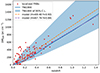 |
Fig. 1. DMIGM-z relation for localized FRBs. The red dots show localized FRBs. The blue line corresponds to the DMIGM from the IllustrisTNG 300 simulation, and the blue shaded area is the 95% confidence region. The dashed orange and purple lines represent the models in Equation (5) with different parameters (H0 and fIGM). 〈DMIGM〉 = DMexc–〈DMhost〉, where 〈DMhost〉 is given by the IllustrisTNG simulation. |
To run a Markov chain Monte Carlo (MCMC) simulation, we calculated the probability distribution of extragalactic DM components. DMhost follows a lognormal distribution (Macquart et al. 2020; Zhang et al. 2020)
![Mathematical equation: $$ p_{\mathrm {host}}\left ({\mathrm {DM_{host}}}\right ) = \frac {1}{\sqrt {2\pi }\ {\mathrm {DM_{host}}}\ \sigma _{\mathrm {host}}} \exp \left [-\frac {(\ln {\mathrm {DM_{host}}}-\mu )^{2}}{2 \sigma _{\mathrm {host}}^{2}}\right ], $$](/articles/aa/full_html/2025/06/aa53006-24/aa53006-24-eq9.gif) (6)
(6)
where eμ is the mean of the distribution. DMIGM can be fit with a Gaussian-like distribution, which is written as (Macquart et al. 2020; Zhang et al. 2021)
![Mathematical equation: $$ p_{\mathrm {IGM}}(\Delta ) = A \Delta ^{-\beta } \exp \left [-\frac {\left (\Delta ^{-\alpha }-C_{0}\right )^{2}}{2 \alpha ^{2} \sigma _{\mathrm {IGM}}^{2}}\right ],\ \Delta =\frac {\mathrm {DM_{IGM}}}{\langle {\mathrm {DM_{IGM}}}\rangle }, $$](/articles/aa/full_html/2025/06/aa53006-24/aa53006-24-eq10.gif) (7)
(7)
where α=β = 3 (Macquart et al. 2020). A and C0 are the normalization parameters given by ∫pIGM = 1 and 〈Δ〉 = 1.
Previous works were made with similar MCMC methods (James et al. 2022; Kalita et al. 2025). They fit all free parameters simultaneously. The probability function is p∼phost(DM∣eμ,σhost,H0) pIGM(DM∣σIGM,H0). Since the number of localized FRBs is small (nlocal∼100 currently, and nlocal<20 for earlier researches), the confidence is significantly weakened to fit four parameters (eμ,σhost,σIGM,H0) simultaneously. Previous works also assumed that the distribution parameters were fixed constants for different FRBs, but some showed a dependence on redshift.
To reduce the size of the parameter space, we used the probability distributions derived from the IllustrisTNG simulation. Zhang et al. (2020) and Zhang et al. (2021) derived the best-fit distribution parameters of DMhost and DMIGM from the IllustrisTNG simulation (Pillepich et al. 2017). To apply the results from IllustrisTNG simulation, all localized FRBs were divided roughly into three categories based on the properties of the host galaxies: Nonrepeating bursts, FRB121102-like repeating bursts, and FRB180916-like repeating bursts. Zhang et al. (2020) and Zhang et al. (2021) provided the best-fit values of the distribution parameters (eμ,σhost,σIGM,A,and C0) in Equations (6) and (7) at several redshifts. We performed a monotone cubic spline interpolation for each parameter to obtain the values at any given redshift.
Taking all parameters into Equations (6) and (7), we obtained the likelihood function for one FRB,
 (8)
(8)
The parameters of the DMhost and DMIGM distributions in Equation (8) are different for each FRB. For the ith FRB, the complete likelihood function is
 (9)
(9)
The total log-likelihood function of all FRBs is
 (10)
(10)
We used a uniform distribution  km s−1 Mpc−1as prior.
3.2. MCMC sampling of localized FRBs
3.2.1. Data preprocessing
To run the MCMC sampling, we used the open-source Python package emcee (Goodman & Weare 2010). We adopted fIGM = 0.93,DMhalo = 65 pc cm−3 and the cosmological parameters given by Planck Collaboration VI (2020). The statistical error of these parameters is discussed in Section 5. Before the initialization of MCMC, the observation data were preprocessed. The preprocessing included the steps listed below.
(a) We calculated the Galactic component of DMs and subtracted it from the total DM to obtain DMexc.
(b) We performed monotone cubic spline interpolations on the data from Zhang et al. (2020, 2021) and calculated the distribution parameters involved in Equation (9) for each FRB.
(c) We set the initial positions for the MCMC walkers. A universal choice for the initialization is to uniformly scatter walkers in a small sphere around the optimal value given by a maximum likelihood estimation (MLE). We tested intervals with a length of 10−3 km s−1 Mpc−1 centered at different values within [60,80] km s−1 Mpc−1, and we found that the initialization has little influence on the constraint result and converged within 30 MCMC steps. We used  km s−1 Mpc−1 as our final initialization.
3.2.2. Monte Carlo cycle and postprocessing
We set up a Monte Carlo system with 512 walkers. In each Monte Carlo cycle, the program went through the steps listed below.
(a) We calculated the mean value of DMIGMwith the current H0 based on Equation (5) for each FRB.
(b) For any given DMhost, we calculated phost(DMhost) and pIGM(Δ) based on Equations (6) and (7), and integrated DMhost to obtain the likelihood function ℒFRB according to Equation (8) for each FRB.
(c) We summed the log-likelihood functions of all FRBs and updated H0 based on the total likelihood.
The autocorrelation time τf is a typical value that is integrated from the autocorrelation function (ACF) to indicate whether the system converges. The documentation of emcee and Goodman & Weare (2010) suggests that N>50τ is long enough, where N is the length of the MCMC chain. We ran a chain of 2000 steps, and the autocorrelation time was τ = 24.66. We discarded the first ⌈τ+50⌉ steps, which may not converge well, and flattened the following steps to obtain a total of 1925×512 = 985 600 samples.
3.2.3. Results of the localized FRBs
The histogram of all samples is plotted with a bin-width chosen by the Freedman Diaconis rule implemented by numpy. The probability density function (PDF) is given by the kernel density estimation (KDE). We also plot the cumulative histogram to obtain the cumulative distribution function (CDF). The best fit is  km s−1 Mpc−1, with a 1σ confidence interval, as shown in Fig. 2. Our constraint from localized FRBs lies between the early-time result given by Planck Collaboration VI (2020) and the late-time result given by Riess et al. (2022).
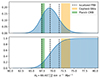 |
Fig. 2. Probability density function and cumulative distribution function of H0 given by 108 localized FRBs. The vertical line shows our result |
Moreover, we tried to divide the FRBs into several bins to investigate the value of H0 at different redshifts, similar as (Krishnan et al. 2020; Jia et al. 2023, 2025; Hu & Wang 2023; Colgáin 2024). We divided the FRBs into two bins and determined an apparently descending trend, which is not significant. When we tried to divide the sample into more bins, the values became unstable and highly sensitive to the selection of a single FRB. This might be caused by the limited number and uneven distribution of the FRBs.
4. Constraint with nonlocalized FRBs
Although the number of localized FRBs is increasing rapidly, most FRBs still remain nonlocalized. It is therefore crucial to use nonlocalized FRBs. A possible solution is to inverse the pseudo-redshifts with the observed DM (Tang et al. 2023). Compared with another method such as generating FRB data with simulation, FRBs with pseudo-redshifts are not dependent on any assumption of the DM distribution because we use real DM data as its foundation. We used all bursts in the first CHIME3 catalog (CHIME/FRB Collaboration 2021) and part of the available repeating bursts with definite coordinates in the CHIME catalog 2023 (CHIME/FRB Collaboration 2023) to run the MCMC sampling. When we processed the repeating FRBs, we considered all bursts from the same source as one single eventd and calculate their mean DM as DMobs. With the pseudo-redshifts, we used all nonlocalized FRBs as localized FRBs to constrain H0.
4.1. Redshift distribution
4.1.1. Circular argument
Before the pseudo-redshifts are estimated, an assumed value for H0 is required. This is a circular argument. However, it can be considered as an iterative analysis similar to the Newton-Raphson method. We assumed an initial value  to calculate the pseudo-redshifts z(0) in the first iteration, and we applied z(0) to estimate
  . To be precise, this step should be repeated as
 (11)
(11)
until  . Through the MCMC sampling, we found that different initial values of H0 affect the pseudo-redshifts and the final estimation of H0 only little.
Another way to avoid a circular argument is to consider H0 as an unfit parameter (same as the pseudo-redshift) instead of assuming its value. To guarantee that the estimated H0 is the same for all FRBs, the pseudo-redshifts must be simultaneously computed for all FRBs, that is, (H0,z1,z2,⋯,zn) must be fit simultaneously. For n = 527, an enormous computational resource is required to fit a 528-dimensional parameter space. We used the first method.
4.1.2. Calculating the redshift distribution
The pseudo-redshifts can be estimated with two different methods: the maximum likelihood estimation (MLE), and a Monte Carlo sampling. Both methods require a likelihood function that is slightly different from Equation (8). H0 is a known parameter, and zi is the parameter we need to fit. The equation is rewritten as
 (12)
(12)
The MLE can give the mean value of pseudo-redshift for each FRB. The chain may fail to converge for FRBs with low DMexc, and MLE gives no information about its distribution. The Monte Carlo sampling provides the probability density distribution and works for FRBs with a low DM. As a result, we used a Monte Carlo sampling instead of the MLE.
With a similar MCMC sampling as described in Section 3.2.2, 57 600 samples (nwalkers = 64, discard = 100, steps = 1000) were generated for each FRB. We calculated the 16, 50, and 84 percentiles (1σ confidence) of the pseudo-redshift for each FRB and plot them in the form of error bars on a scatter plot with the DM as the horizontal axis. For any given percentile (e.g., z16,z50, or z84), z∼DMexc shows a good linear relation that agrees with the pseudo-redshifts from previous research. We plot the result of the linear regression and show the 68% confidence region in Fig. 3 and Fig. 4.
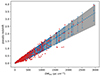 |
Fig. 3. Pseudo-redshifts of nonlocalized FRBs in the first CHIME catalog. The blue dots with the error bars are the median values and 1σ confidence interval of redshifts estimated with the MCMC method. The dashed blue line and gray region were fitted from the blue dots. The red dots are the pseudo-redshifts (see Section 4.2.1), which were decided randomly based on the PDF given by the MCMC sampling for each FRB. Extreme MCMC samples were neglected. |
4.2. MC sampling of nonlocalized FRBs
4.2.1. Generating the pseudo-redshifts
The pseudo-redshifts have an intrinsic difference from real redshifts of FRBs. The errors of the real redshifts are negligible. However, the distribution of the pseudo-redshifts could not be constrained within a small confidence interval. It is insufficient to simply use an error bar or Gaussian distribution around the peak value to describe pseudo-redshifts.
We assigned a pseudo-redshift within a relatively large interval for each FRB based on its PDF. It is located near the peak with a high probability and lies far away from the peak with a very low probability. When we repetitively generated this hundreds of times, all these pseudo-redshifts reflected the PDF well. Although we were unable to generate multiple times for one FRB during the sampling, we were able to generate once for each FRB, and we had 527 FRBs. It is statistically safe to reflect their PDFs, and this is exactly how real redshifts are like. Furthermore, we did not consider an error bar of the pseudo-redshift because an error bar is insufficient to describe the PDF.
There is a small possibility that the generated redshift is very far away from the peak. To avoid this extreme situation, we discarded generated redshifts that lay outside 94% of the region that was centered the peak (i.e., below 3% and above 97% in the PDF) and regenerate again. The pseudo-redshifts are shown as red dots in Fig. 3 and Fig. 4.
4.2.2. H0 from nonlocalized FRBs
We ran an MCMC sampling similar to Section 3 using the pseudo-redshifts as described in Section 4.2.1. The result was  km s−1 Mpc−1, as shown in Fig. 5. The median value given by nonlocalized FRBs is very close to that given by localized FRBs. Moreover, since the redshifts are pseudo, the uncertainty of the result from the nonlocalized FRBs is much more inspiring than the median value. It provides a convincing prediction that if 527 FRBs are localized, the uncertainty drops to ∼1% at a confidence level of 1σ. Compared with the result of localized FRBs, we have err1/err2 = 3.02 and
  . The ratio is roughly consistent with the relation
  .
.
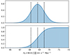 |
Fig. 5. PDF and CDF of the H0 given by the pseudo-redshifts of nonlocalized FRBs. The vertical line shows the result |

5. Discussion
By using the pseudo-redshifts of 527 nonlocalized CHIME FRBs, we significantly reduced the uncertainty of the constraint. However, some bias and errors must be included for a full discussion. We generally divide them into the statistical and the systematic error.
5.1. Statistical errors
The statistical error mainly refers to the error of the cosmological parameters Ωbh2 and Ωm in Equation (5). Other constants such as G and mp are already measured with extremely high precision. Planck Collaboration VI (2020) gave Ωbh2 = 0.02242±0.00014 and Ωm = 0.3111±0.0056.
For Ωbh2, it appears in Equation (5) as a linear term with H0. Assuming a Gaussian distribution p(x) of about μ = 0.02242, we roughly estimated
 (13)
(13)
which means that if Ωbh2 follows a symmetric distribution (e.g., a Gaussian distribution), it affects H0 only weakly. Furthermore, the error of Ωbh2 (∼0.6%) is much smaller than for other terms such as Ωm, and it is also smaller than the result of our constraint (ΔH0/H0∼0.94%). As a result, it is safe to ignore the error of Ωbh2.
For Ωm, which appears inside the integral in Equation (5), the uncertainty is ∼1.8% and cannot be ignored. To marginalize Ωm, the best way is to add another level of integral, which would significantly increase the computation time. Alternatively, we considered replacing the integral with an expansion. We assumed a Gaussian distribution p(x) with μ = 0.3111 and σ = 0.0056. The integral can then be written as
![Mathematical equation: $$ \begin{aligned} I&=\int _{-\infty }^{\infty } p(x)\int _{0}^{Z} \frac {(1+z)}{\left [x(1+z)^{3} + 1 - x \right ]^{1 / 2}}{\mathrm {d}}z{\mathrm {d}}x\\ &\simeq \int _{0}^{Z}\frac {(1+z)}{I_0}\int _{\mu -\sigma }^{\mu +\sigma } \frac {p(x) }{\left [x(1+z)^{3} + 1 - x \right ]^{1 / 2}}{\mathrm {d}}x{\mathrm {d}}z\\ &\equiv \int _{0}^{Z}\frac {(1+z)}{I_0}\int _{\mu -\sigma }^{\mu +\sigma }f(x,z){\mathrm {d}}x{\mathrm {d}}z, \end{aligned} $$](/articles/aa/full_html/2025/06/aa53006-24/aa53006-24-eq28.gif) (14)
(14)
where  is the normalization factor and
 ![Mathematical equation: $ f(x,z) = p(x)/\left [x(1+z)^{3} + 1 - x \right ]^{1 / 2} $](/articles/aa/full_html/2025/06/aa53006-24/aa53006-24-eq30.gif) is our target function. Z is the redshift of an FRB, and z is our integration variable. Since both ∫f(x,z)dx and ∫f(x,z)dz cannot be expressed by elementary functions, we performed a series expansion on f(x,z)dz around x=μ and obtained
is our target function. Z is the redshift of an FRB, and z is our integration variable. Since both ∫f(x,z)dx and ∫f(x,z)dz cannot be expressed by elementary functions, we performed a series expansion on f(x,z)dz around x=μ and obtained  . We plot the figure of g(x,z) at different z and compare it with the original function to ensure that the expansion is acceptable. The inner integral in Equation (14) can then be written as an explicit function of z, that is,
  . However, the form of h(z) is still too complicated for an integration, and we thus needed to perform another series expansion around z=z0. To determine the best value for z0, we plot the expanded function at different z0 and degrees. An expansion of h(z) to the term of (z−z0)4 around z0 = 2.5 provides best fit for both z→0 and z→4. We denote it as
  , and we can complete the whole integral: I≃1.02 Z+0.19 Z2−0.14 Z3+0.043 Z4−0.0066 Z5+0.00042 Z6.
Taking the new expression into Equation (5), we ran the MCMC sampling with Ωm marginalized. The result is shown in Fig. 6 (the method in Section 4.2.1 was used). H0 is  km s−1 Mpc−1 in 1σ confidence intervals, which is consistent with the previous result in Fig. 5. Therefore, the statistical error of Ωm does not influence the constraint on H0 significantly.
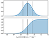 |
Fig. 6. PDF and CDF of H0 considering the statistical error of Ωm using the pseudo-redshifts of nonlocalized FRBs. The vertical line shows the result |
5.2. Systematic errors
Several systematic errors need to be discussed. In Equation (5), compared with Ωbh2 and Ωm, the fraction of baryons in IGM fIGM may introduce more uncertainty. However, we still know little about fIGM. Shull et al. (2012) gave a value of ∼0.84. Connor et al. (2024) provided a more accurate constraint of ∼0.93, which depends on the models. Khrykin et al. (2024) gave a lower value of  based on the FLIMFLAM spectroscopic survey. Current research is clearly still undetermined. Furthermore, it is difficult to separate the error of fIGM from H0 as they appear in a coupling term fIGM/H0 in Equation (5). To be precise, only a constraint on fIGM/H0 can be made instead of a constraint on H0. The value of H0 must therefore be determined by other approaches when fIGM is constrained from FRBs. By fixing H0, it has been found that the uncertainty of fIGM is about 8% (Yang et al. 2022; Connor et al. 2024). The systematic error from fIGM clearly currently dominates the error of the measured H0. On the other hand, it may vary with redshift. Without further independent constraints on fIGM, we cannot exclude the error of fIGM. Trying to marginalize fIGM with a Gaussian distribution during the MCMC sampling was unable to provide a more accurate value of H0. It only gives
  where
where  is the error assumed in the Gaussian distribution. More research with other methods is required to further investigate the error of fIGM.
DMhost includes all contributions to the DM that come from the host galaxy. Based on IllustrisTNG simulations, the probability distribution of DMhostincluding the local cosmic structure (e.g., filament) halo and interstellar medium of the host were derived (Zhang et al. 2020). However, the vicinity of FRB progenitors was not considered. The most promising progenitors of FRBs are young magnetars (Wang & Yu 2017), which can be formed by the core collapse of massive stars or by mergers of two compact objects (Wang et al. 2020). They might therefore be embedded in a magnetar wind nebula and supernova remnant (Yang & Zhang 2017; Piro & Gaensler 2018; Zhao & Wang 2021). On the other hand, the large DMhostwith a rotation measure reversal for FRB 20190520B indicates that it might reside in a binary system (Wang et al. 2022; Anna-Thomas et al. 2023). Similar FRBs should therefore be removed when measuring H0. For FRBs with little DM contribution from the vicinity, a precise modeling should be performed. It is important to use optical observations of the FRB host galaxy environment, combined with the rotation measure and the scattering times of FRBs to constrain DMhost (Cordes et al. 2022).
DMIGM refers to the entire DM contribution between the host galaxy and the Milky Way, which includes contributions from the IGM and other intervening galaxy groups and halos. It is difficult to determine the number of intervening galaxies because the randomness is significant, and it is even more difficult to identify the stellar mass and SFR for each galaxy, which is greatly relevant to the relating DM. Connor et al. (2024) tried to separate the contribution of the IGM and halos and reported a corresponding baryon fraction. Because we chose their value of fIGM, it contains the baryon from the IGM and halos, which can be considered as a statistical average to compensate for the unknown intervening galaxies.
Several selection biases should be discussed, such as the signal-to-noise ratio (S/N) effect, the ISM effect, the selection effect of nonlocalized FRBs, and the gridding effect (James et al. 2022). For the selection effect of nonlocalized FRBs, our constraint has no such error because we made use of most nonlocalized FRBs in the CHIME database. For the gridding effect, we used continuous values for redshifts and DMs instead of discrete variables. For the S/N effect, the log-log figure of a number of events observed above the S/N threshold should follow a power law of –1.5 (in the log-log plot, i.e., N∝S/N−1.5), and James et al. (2022) found that events from CRAFT/ICS deviate from the –1.5 power law. We plot the same figure with nonlocalized FRBs from the CHIME database in Fig. 7. The histogram followed the power law well, and our constraint is therefore not much influenced by the S/N effect. For the ISM effect, James et al. (2022) claimed that DMISMwould increase at low galactic latitudes, which may prevent telescopes from observing these events. We plot the Hammer projection of FRBs in the galactic coordinate system in Fig. 8. A Hammer projection is an equal-area projection, and a considerable number of FRBs are located in low galactic latitude areas. Furthermore, a few of these low-galactic-latitude FRBs have shown high values of DMISM. Only one of the 108 localized FRBs has DMISM> 200 pc cm−3, but the largest observed DM is about 1500 pc cm−3. It is not likely that FRBs are missed by observations because DMISM is too high.
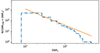 |
Fig. 7. Signal-to-noise ratio for one-off FRBs in the first CHIME catalog where repeating FRBs are not counted. The yellow line with a slope of −1.5 (in log-log scale) was not fit by the data and is shown just for comparison. |
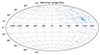 |
Fig. 8. Hammer projection of the FRB distribution in the first CHIME catalog in the galactic coordinate system. Repeating FRBs are only counted once. |
6. Conclusions
We ran an MCMC sampling to constrain H0 using 108 localized FRBs and 527 nonlocalized FRBs from the CHIME catalog. We applied the redshift-DM relation and a Bayesian estimation to build the MCMC model. We used normalization factors obtained from the IllustrisTNG simulation to model the DM distribution. For localized FRBs, we obtained  km s−1 Mpc−1 with 108 FRBs, which lies between constraints from late- and early-time research. For nonlocalized FRBs, we ran individual MCMC samplings instead of a maximum likelihood estimation to obtain a probability density distribution of the pseudo-redshift for each FRB. We assigned pseudo-redshifts for FRBs and obtained
  km s−1 Mpc−1.
The statistical errors of the cosmological parameters, the systematic error of fIGM, and the selection biases were discussed. We showed that the statistical error of Ωb affects our constraint less than Ωm. We performed a series expansion to marginalize Ωm and obtained  km s−1 Mpc−1. The degeneracy effect prevented us from separating the error of fIGM from H0. The uncertainty of H0 is dominated by the error of the fraction of cosmic baryons in the diffuse ionized gas fIGM. Other systematic errors were neglected.
Our study predicts future constraints on H0 with more localized FRBs. Our result shows that the uncertainty of H0 is likely to drop to ∼1% when the number of localized FRBs increases to ∼500. FRBs will become a powerful tool for solving the Hubble tension.
Acknowledgments
We thank the anonymous referee for constructive comments. This work was supported by the National Natural Science Foundation of China (grant Nos. 12494575, 12273009 and 12393812), the National SKA Program of China (grant Nos. 2020SKA0120302 and 2022SKA0130100), and the Natural Science Foundation of Xinjiang Uygur Autonomous Region (grant No. 2023D01E20).
FRB Line-of-sight Ionization Measurement From Lightcone AAOmega Mapping.
Fast and Fortunate for FRB Follow-up.
The Canadian Hydrogen Intensity Mapping Experiment.
References
- Amiri, M., Amouyal, D., Andersen, B. C., et al. 2025, ArXiv e-prints [arXiv:2502.11217] [Google Scholar]
- Anna-Thomas, R., Connor, L., Dai, S., et al. 2023, Science, 380, 599 [NASA ADS] [CrossRef] [Google Scholar]
- Anna-Thomas, R., Law, C. J., Koch, E. W., et al. 2025, ApJ, submitted [arXiv:2503.02947] [Google Scholar]
- Bannister, K. W., Deller, A. T., Phillips, C., et al. 2019, Science, 365, 565 [NASA ADS] [CrossRef] [Google Scholar]
- Bhandari, S., & Flynn, C. 2021, Universe, 7, 85 [Google Scholar]
- Bhandari, S., Sadler, E. M., Prochaska, J. X., et al. 2020, ApJ, 895, L37 [NASA ADS] [CrossRef] [Google Scholar]
- Bhandari, S., Heintz, K. E., Aggarwal, K., et al. 2022, AJ, 163, 69 [NASA ADS] [CrossRef] [Google Scholar]
- Bhandari, S., Gordon, A. C., Scott, D. R., et al. 2023, ApJ, 948, 67 [NASA ADS] [CrossRef] [Google Scholar]
- Bhardwaj, M., Kirichenko, A. Y., Michilli, D., et al. 2021, ApJ, 919, L24 [NASA ADS] [CrossRef] [Google Scholar]
- Bhardwaj, M., Michilli, D., Kirichenko, A. Y., et al. 2024, ApJ, 971, L51 [Google Scholar]
- Caleb, M., Driessen, L. N., Gordon, A. C., et al. 2023, MNRAS, 524, 2064 [NASA ADS] [CrossRef] [Google Scholar]
- Cassanelli, T., Leung, C., Sanghavi, P., et al. 2024, Nat. Astron., 8, 1429 [Google Scholar]
- Chatterjee, S., Law, C. J., Wharton, R. S., et al. 2017, Nature, 541, 58 [NASA ADS] [CrossRef] [Google Scholar]
- CHIME/FRB Collaboration (Amiri, M., et al.) 2021, ApJS, 257, 59 [NASA ADS] [CrossRef] [Google Scholar]
- CHIME/FRB Collaboration (Andersen, B. C., et al.) 2023, ApJ, 947, 83 [NASA ADS] [CrossRef] [Google Scholar]
- Chittidi, J. S., Simha, S., Mannings, A., et al. 2021, ApJ, 922, 173 [NASA ADS] [CrossRef] [Google Scholar]
- Colgáin, Ó. E., Sheikh-Jabbari, M. M., Solomon, R., Dainotti, M. G., & Stojkovic, D., 2024, Phys. Dark Univ., 44, 101464 [Google Scholar]
- Connor, L., Ravi, V., Sharma, K., et al. 2024, ArXiv e-prints [arXiv:2409.16952] [Google Scholar]
- Cooke, R. J., Pettini, M., & Steidel, C. C. 2018, ApJ, 855, 102 [Google Scholar]
- Cordes, J. M., & Chatterjee, S. 2019, ARA&A, 57, 417 [NASA ADS] [CrossRef] [Google Scholar]
- Cordes, J. M., & Lazio, T. J. W. 2002, ArXiv e-prints [arXiv:astroph/0207156] [Google Scholar]
- Cordes, J. M., Ocker, S. K., & Chatterjee, S. 2022, ApJ, 931, 88 [NASA ADS] [CrossRef] [Google Scholar]
- Driessen, L. N., Barr, E. D., Buckley, D. A. H., et al. 2023, MNRAS, 527, 3659 [NASA ADS] [CrossRef] [Google Scholar]
- Freedman, W. L. 2021, ApJ, 919, 16 [NASA ADS] [CrossRef] [Google Scholar]
- Gao, J., Zhou, Z., Du, M., et al. 2024, MNRAS, 527, 7861 [Google Scholar]
- Goodman, J., & Weare, J. 2010, Comm App Math Comp Sci., 5, 65 [Google Scholar]
- Gordon, A. C., Fong, W. -F., Kilpatrick, C. D., et al. 2023, ApJ, 954, 80 [NASA ADS] [CrossRef] [Google Scholar]
- Hagstotz, S., Reischke, R., & Lilow, R. 2022, MNRAS, 511, 662 [CrossRef] [Google Scholar]
- Heintz, K. E., Prochaska, J. X., Simha, S., et al. 2020, ApJ, 903, 152 [NASA ADS] [CrossRef] [Google Scholar]
- Hu, J. -P., & Wang, F. -Y. 2023, Universe, 9, 94 [CrossRef] [Google Scholar]
- Huang, Y., Simha, S., Khrykin, I. S., et al. 2025, ApJS, 277, 64 [Google Scholar]
- Hubble, E. 1929, Proc. Natl. Acad. Sci., 15, 168 [Google Scholar]
- Ibik, A. L., Drout, M. R., Gaensler, B. M., et al. 2024, ApJ, 961, 99 [NASA ADS] [CrossRef] [Google Scholar]
- James, C. W., Ghosh, E. M., Prochaska, J. X., et al. 2022, MNRAS, 516, 4862 [NASA ADS] [CrossRef] [Google Scholar]
- Jia, X. D., Hu, J. P., & Wang, F. Y. 2023, A&A, 674, A45 [NASA ADS] [CrossRef] [EDP Sciences] [Google Scholar]
- Jia, X. D., Hu, J. P., Yi, S. X., & Wang, F. Y. 2025, ApJ, 979, L34 [Google Scholar]
- Kalita, S., Bhatporia, S., & Weltman, A. 2025, Phys. Dark Univ., 48, 101926 [Google Scholar]
- Keane, E. F., Stappers, B. W., Kramer, M., & Lyne, A. G. 2012, MNRAS, 425, L71 [NASA ADS] [CrossRef] [Google Scholar]
- Keating, L. C., & Pen, U. -L. 2020, MNRAS, 496, L106 [NASA ADS] [CrossRef] [Google Scholar]
- Khrykin, I. S., Ata, M., Lee, K. -G., et al. 2024, ApJ, 973, 151 [Google Scholar]
- Kirsten, F., Marcote, B., Nimmo, K., et al. 2022, Nature, 602, 585 [NASA ADS] [CrossRef] [Google Scholar]
- Krishnan, C., Colgáin, E. Ó., Ruchika, T., et al. 2020, Phys. Rev. D, 102, 103525 [NASA ADS] [CrossRef] [Google Scholar]
- Law, C. J., Butler, B. J., Prochaska, J. X., et al. 2020, ApJ, 899, 161 [NASA ADS] [CrossRef] [Google Scholar]
- Law, C. J., Sharma, K., Ravi, V., et al. 2024, ApJ, 967, 29 [NASA ADS] [CrossRef] [Google Scholar]
- Lee, K. -G., Ata, M., Khrykin, I. S., et al. 2022, ApJ, 928, 9 [NASA ADS] [CrossRef] [Google Scholar]
- Lee, K. -G., Khrykin, I. S., Simha, S., et al. 2023, ApJ, 954, L7 [NASA ADS] [CrossRef] [Google Scholar]
- Lin, H. -N., & Zou, R. 2023, MNRAS, 520, 6237 [Google Scholar]
- Lorimer, D. R., Bailes, M., McLaughlin, M. A., Narkevic, D. J., & Crawford, F. 2007, Science, 318, 777 [Google Scholar]
- Macquart, J. P., Prochaska, J. X., McQuinn, M., et al. 2020, Nature, 581, 391 [Google Scholar]
- Mahony, E. K., Ekers, R. D., Macquart, J. -P., et al. 2018, ApJ, 867, L10 [Google Scholar]
- Marcote, B., Nimmo, K., Hessels, J. W. T., et al. 2020, Nature, 577, 190 [NASA ADS] [CrossRef] [Google Scholar]
- Michilli, D., Bhardwaj, M., Brar, C., et al. 2023, ApJ, 950, 134 [NASA ADS] [CrossRef] [Google Scholar]
- Niu, C. -H., Aggarwal, K., Li, D., et al. 2022, Nature, 606, 873 [NASA ADS] [CrossRef] [Google Scholar]
- Petroff, E., Hessels, J. W. T., & Lorimer, D. R. 2022, A&ARv, 30, 2 [NASA ADS] [CrossRef] [Google Scholar]
- Pillepich, A., Springel, V., Nelson, D., et al. 2017, MNRAS, 473, 4077 [Google Scholar]
- Piro, A. L., & Gaensler, B. M. 2018, ApJ, 861, 150 [NASA ADS] [CrossRef] [Google Scholar]
- Planck Collaboration VI. 2020, A&A, 641, A6 [NASA ADS] [CrossRef] [EDP Sciences] [Google Scholar]
- Prochaska, J. X., & Zheng, Y. 2019, MNRAS, 485, 648 [NASA ADS] [Google Scholar]
- Prochaska, J. X., Macquart, J. -P., McQuinn, M., et al. 2019, Science, 366, 231 [NASA ADS] [CrossRef] [Google Scholar]
- Rajwade, K. M., Bezuidenhout, M. C., Caleb, M., et al. 2022, MNRAS, 514, 1961 [Google Scholar]
- Rajwade, K. M., Driessen, L. N., Barr, E. D., et al. 2024, MNRAS, 532, 3881 [Google Scholar]
- Ravi, V., Catha, M., D’Addario, L., et al. 2019, Nature, 572, 352 [NASA ADS] [CrossRef] [Google Scholar]
- Ravi, V., Law, C. J., Li, D., et al. 2022, MNRAS, 513, 982 [CrossRef] [Google Scholar]
- Ravi, V., Catha, M., Chen, G., et al. 2023, ApJ, 949, L3 [NASA ADS] [CrossRef] [Google Scholar]
- Ravi, V., Catha, M., Chen, G., et al. 2025, AJ, 169, 330 [Google Scholar]
- Riess, A. G., Yuan, W., Macri, L. M., et al. 2022, ApJ, 934, L7 [NASA ADS] [CrossRef] [Google Scholar]
- Ryder, S. D., Bannister, K. W., Bhandari, S., et al. 2023, Science, 382, 294 [NASA ADS] [CrossRef] [Google Scholar]
- Shannon, R. M., Bannister, K. W., Bera, A., et al. 2025, PASA, 42, e036 [Google Scholar]
- Sharma, K., Ravi, V., Connor, L., et al. 2024, Nature, 635, 61 [Google Scholar]
- Shull, J. M., Smith, B. D., & Danforth, C. W. 2012, ApJ, 759, 23 [NASA ADS] [CrossRef] [Google Scholar]
- Simha, S., Tejos, N., Prochaska, J. X., et al. 2021, ApJ, 921, 134 [NASA ADS] [CrossRef] [Google Scholar]
- Tang, L., Lin, H. -N., & Li, X. 2023, Chin. Phys. C, 47, 085105 [Google Scholar]
- Tendulkar, S. P., Bassa, C. G., Cordes, J. M., et al. 2017, ApJ, 834, L7 [NASA ADS] [CrossRef] [Google Scholar]
- Thornton, D., Stappers, B., Bailes, M., et al. 2013, Science, 341, 53 [NASA ADS] [CrossRef] [Google Scholar]
- Valentino, E. D., Mena, O., Pan, S., et al. 2021, CQG, 38, 153001 [NASA ADS] [CrossRef] [Google Scholar]
- Wang, B., & Wei, J. -J. 2023, ApJ, 944, 50 [NASA ADS] [CrossRef] [Google Scholar]
- Wang, F. Y., & Yu, H. 2017, JCAP, 03, 023 [CrossRef] [Google Scholar]
- Wang, F. Y., Wang, Y. Y., Yang, Y. -P., et al. 2020, ApJ, 891, 72 [NASA ADS] [CrossRef] [Google Scholar]
- Wang, F. Y., Zhang, G. Q., Dai, Z. G., & Cheng, K. S. 2022, Nat Commun., 13, 4382 [Google Scholar]
- Wei, J. -J., & Melia, F. 2023, ApJ, 955, 101 [Google Scholar]
- Wu, Q., & Wang, F. -Y. 2024, Chin. Phys. Lett., 41, 119801 [NASA ADS] [CrossRef] [Google Scholar]
- Wu, Q., Yu, H., & Wang, F. Y. 2020, ApJ, 895, 33 [NASA ADS] [CrossRef] [Google Scholar]
- Wu, Q., Zhang, G. -Q., & Wang, F. -Y. 2022, MNRAS, 515, L1 [NASA ADS] [CrossRef] [Google Scholar]
- Xiao, D., Wang, F., & Dai, Z. 2021, Sci. China Phys. Mech. Astron., 64, 249501 [NASA ADS] [CrossRef] [Google Scholar]
- Yang, Y. -P., & Zhang, B. 2017, ApJ, 847, 22 [Google Scholar]
- Yang, K. B., Wu, Q., & Wang, F. Y. 2022, ApJ, 940, L29 [NASA ADS] [CrossRef] [Google Scholar]
- Yao, J. M., Manchester, R. N., & Wang, N. 2017, ApJ, 835, 29 [NASA ADS] [CrossRef] [Google Scholar]
- Zhang, B. 2023, Rev. Mod. Phys., 95, 035005 [NASA ADS] [CrossRef] [Google Scholar]
- Zhang, G. Q., Yu, H., He, J. H., & Wang, F. Y. 2020, ApJ, 900, 170 [NASA ADS] [CrossRef] [Google Scholar]
- Zhang, Z. J., Yan, K., Li, C. M., Zhang, G. Q., & Wang, F. Y. 2021, ApJ, 906, 49 [NASA ADS] [CrossRef] [Google Scholar]
- Zhao, Z. Y., & Wang, F. Y. 2021, ApJ, 923, L17 [NASA ADS] [CrossRef] [Google Scholar]
Appendix A: FRB data
Properties of localized FRBs.
(continued)
(continued)
All Tables
All Figures
|
Fig. 1. DMIGM-z relation for localized FRBs. The red dots show localized FRBs. The blue line corresponds to the DMIGM from the IllustrisTNG 300 simulation, and the blue shaded area is the 95% confidence region. The dashed orange and purple lines represent the models in Equation (5) with different parameters (H0 and fIGM). 〈DMIGM〉 = DMexc–〈DMhost〉, where 〈DMhost〉 is given by the IllustrisTNG simulation. |
| In the text | |
|
Fig. 2. Probability density function and cumulative distribution function of H0 given by 108 localized FRBs. The vertical line shows our result |
| In the text | |
|
Fig. 3. Pseudo-redshifts of nonlocalized FRBs in the first CHIME catalog. The blue dots with the error bars are the median values and 1σ confidence interval of redshifts estimated with the MCMC method. The dashed blue line and gray region were fitted from the blue dots. The red dots are the pseudo-redshifts (see Section 4.2.1), which were decided randomly based on the PDF given by the MCMC sampling for each FRB. Extreme MCMC samples were neglected. |
| In the text | |
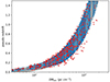 |
Fig. 4. Log scale plot of the pseudo-redshifts in Fig. 3 |
| In the text | |
|
Fig. 5. PDF and CDF of the H0 given by the pseudo-redshifts of nonlocalized FRBs. The vertical line shows the result |
| In the text | |
|
Fig. 6. PDF and CDF of H0 considering the statistical error of Ωm using the pseudo-redshifts of nonlocalized FRBs. The vertical line shows the result |
| In the text | |
|
Fig. 7. Signal-to-noise ratio for one-off FRBs in the first CHIME catalog where repeating FRBs are not counted. The yellow line with a slope of −1.5 (in log-log scale) was not fit by the data and is shown just for comparison. |
| In the text | |
|
Fig. 8. Hammer projection of the FRB distribution in the first CHIME catalog in the galactic coordinate system. Repeating FRBs are only counted once. |
| In the text | |
Current usage metrics show cumulative count of Article Views (full-text article views including HTML views, PDF and ePub downloads, according to the available data) and Abstracts Views on Vision4Press platform.
Data correspond to usage on the plateform after 2015. The current usage metrics is available 48-96 hours after online publication and is updated daily on week days.
Initial download of the metrics may take a while.